Article

Analysis of the Time Series of Compressed Air Flow and Pressure and Determining Criteria for Diagnosing Causes of Pressure Drop in Pneumatic Systems

1
Department of Control Systems, Technical University–Sofia, Branch Plovdiv, 4000 Plovdiv, Bulgaria
2
Center of Competence “Smart Mechatronic, Eco-and Energy-Saving Systems and Technologies”, 4000 Plovdiv, Bulgaria
3
Vocational Training Center TRAKIYA, 4000 Plovdiv, Bulgaria
*
Author to whom correspondence should be addressed.
Appl. Sci. 2025, 15(17), 9536; https://doi.org/10.3390/app15179536 (registering DOI)
Submission received: 20 June 2025 / Revised: 18 July 2025 / Accepted: 27 August 2025 / Published: 29 August 2025

Abstract

This article explores the possibility of diagnosing unwanted pressure drops in pneumatic systems. The proposed algorithm aims to distinguish the causes and location of their occurrence. The diagnostics clearly distinguish pressure drops caused by supply lines from those caused in the main or branch lines of an industrial pneumatic system. Pressure drops in pneumatic systems are one of the main causes of increased energy consumption. For the energy and resource optimization of pneumatic systems, it is essential to detect and locate the causes of pressure drops. This article proposes an approach for using the time diagrams of two measurable variables—flow rate and pressure—at the inlet of the end consumer (machine). Based on constant monitoring and a correlation relationship between the two time series, we determined indicators for detecting and locating unwanted pressure drops. In order to verify the proposed approach and the performed analysis, in general, we made observations of 16 real production machines and lines.

1. Introduction

In modern industry, energy efficiency is a high priority. This is especially true for industrial pneumatic systems, which are critical infrastructure in modern industry, providing over 70% of automated processes [1]. Many studies show that they have huge potential for optimization from an energy point of view. Data show that 20–40% of compressed air in factories is lost [2]. Causes include leaks, poor pressure regulation, pressure drops, oversizing of components, or use of components of questionable quality. This leads to high power consumption, compressor overload, rapid amortization, and high maintenance costs.
Industry 4.0 and smart technologies open up new possibilities. Sensor systems with artificial intelligence and machine learning can collect data for pressure, flow, temperature, and duty cycles in real time. This allows not only monitoring but also automatic optimization.
A key aspect is real-time monitoring and control systems. They dynamically manage energy flows, monitor parameters, predict conditions, warn of deviations, detect leaks, and offer appropriate actions, even automatic corrections [3].
The development requires reliable communication architectures between sensors, control systems, and analytical modules. The system must be scalable for small and large enterprises. The benefits of such an approach are economic and environmental. Power consumption is reduced, equipment life is extended, and unnecessary air losses and carbon footprints are reduced. This is increasingly important for the decarbonization of industry. Although more and more scientific and research papers point out the benefits of focusing on the optimization and maintenance of industrial pneumatic systems, the implementation of such processes in real industry is progressing at a slower rate. The main reason is the lack of sufficiently implemented real-time monitoring tools, poor awareness, and neglect by the management of industrial enterprises.
In the study of [4], an analysis of the possible causes and obstacles to the implementation of effective measures for energy optimization of industrial pneumatic systems is made. The authors list the most common obstacles and barriers to industrial enterprises. After that, often the optimization and elimination of problems in the pneumatic system are not among the main priorities of management, respectively, and the budget of the enterprise, as the main barriers are indicated as the possible cost of diagnosis and assessment of benefits, concerns about long downtimes, and disruption of the production rhythm, as well as additional human labor in diagnosing and eliminating problems.
Increasingly rapid innovations in distributed control, smart metering, and machine learning may encourage companies to implement dynamic energy control [5]. This is especially relevant from the perspective of Industry 4.0.
Analyzing process data and the relationships between different variables gives valuable information. This information is useful for many applications—for example, process monitoring, fault diagnosis, the grouping of operating modes, the monitoring of key or quality variables, and more [6].
From a maintenance perspective, the use of advanced and innovative techniques is also beneficial. They allow for monitoring and controlling performance, as well as monitoring anomalies in energy consumption [7], changes in the production cycles, or changes in other parameters affecting the production process in real time [8,9]. They also assist in the detection and diagnosis of faults [10,11], as well as the assessment of the remaining useful life of the equipment [12]. This is a key point for better production management and maintenance planning.
In operations management, if measured data are compared with an accurate and reliable reference source, it is possible to conduct effective control in real time. This improves system performance and optimizes its operating conditions [13].
Last but not least, the use of real-time control also has economic benefits. By modeling energy characteristics, a more accurate assessment of the energy budget can be made. This allows for the timely detection of anomalies and helps management find their causes. This allows for more effective control over the overall performance and energy efficiency of the system [14,15].
Authors in study [16] show how monitoring the state of a complex system can be achieved with statistical methods. A similar approach to diagnostics and the detection of faults and deviations has been applied by the authors in [17], who even concluded that fault detection in industrial plants is a hot research area, as more and more sensor data are being collected throughout the industrial process. Automatic data-driven approaches are widely needed and seen as a promising area of investment.
The authors in [18] develop a special methodology for real-time energy performance control. The methodology is built on statistical tools for energy measurement and verification, as well as for monitoring and optimizing energy consumption in real time with a special focus on the compressed air system. As additional benefits of applying the methodology, they also point out easier diagnostics and maintenance, as well as the creation of a reliable energy accounting system.
In the main study, researchers have focused their attention on developing methods and systems to detect, locate, and size leaks in pneumatic systems. And this is justified because these leaks generate the vast majority of losses, and their detection is a laborious and time-consuming task.
The authors in [19] propose an automatic system, integrating infrared thermography and computer vision, and have developed an algorithm for automatic localization and the sizing of leaks in end consumers. Through an analysis based on the time for one cycle of the actuators, the authors in [20] offer a method for detecting problems, including the presence of internal or external leaks to the actuator.
In [21], the authors have chosen a statistical approach, looking at the most common causes of leaks and the elements where leaks most often occur within the bottling industry, which serves to assist maintenance managers in prioritizing the replacement of problem elements.
The analysis of time series of pressure P(t) and flow rate Q(t) involves the application of statistical and spectral methods in order to extract characteristic features and dependencies that allow the identification of potential sources of anomalies in pneumatic systems.
Similar diagnostic concepts use techniques such as the cepstrum of cross-correlation between P(t) and Q(t) to identify response delays. This method is used to detect leaks by transient wave analysis [22].
In [23], anomaly detection in pneumatic systems is implemented using statistical methods and time series analysis. Leaks are localized using mathematical indicators on time series. Quantitative analysis involves combining features based on distance measurement techniques in metric space, such as using Minkowski and Canberra distances, as well as correlation techniques, in particular, Pearson’s cross-correlation and angular similarity coefficient.
Maintaining stable operating pressure in industrial compressed air systems is key to energy efficiency, productivity, and equipment longevity.
The pneumatic network provides a supply of compressed air to the point of use.
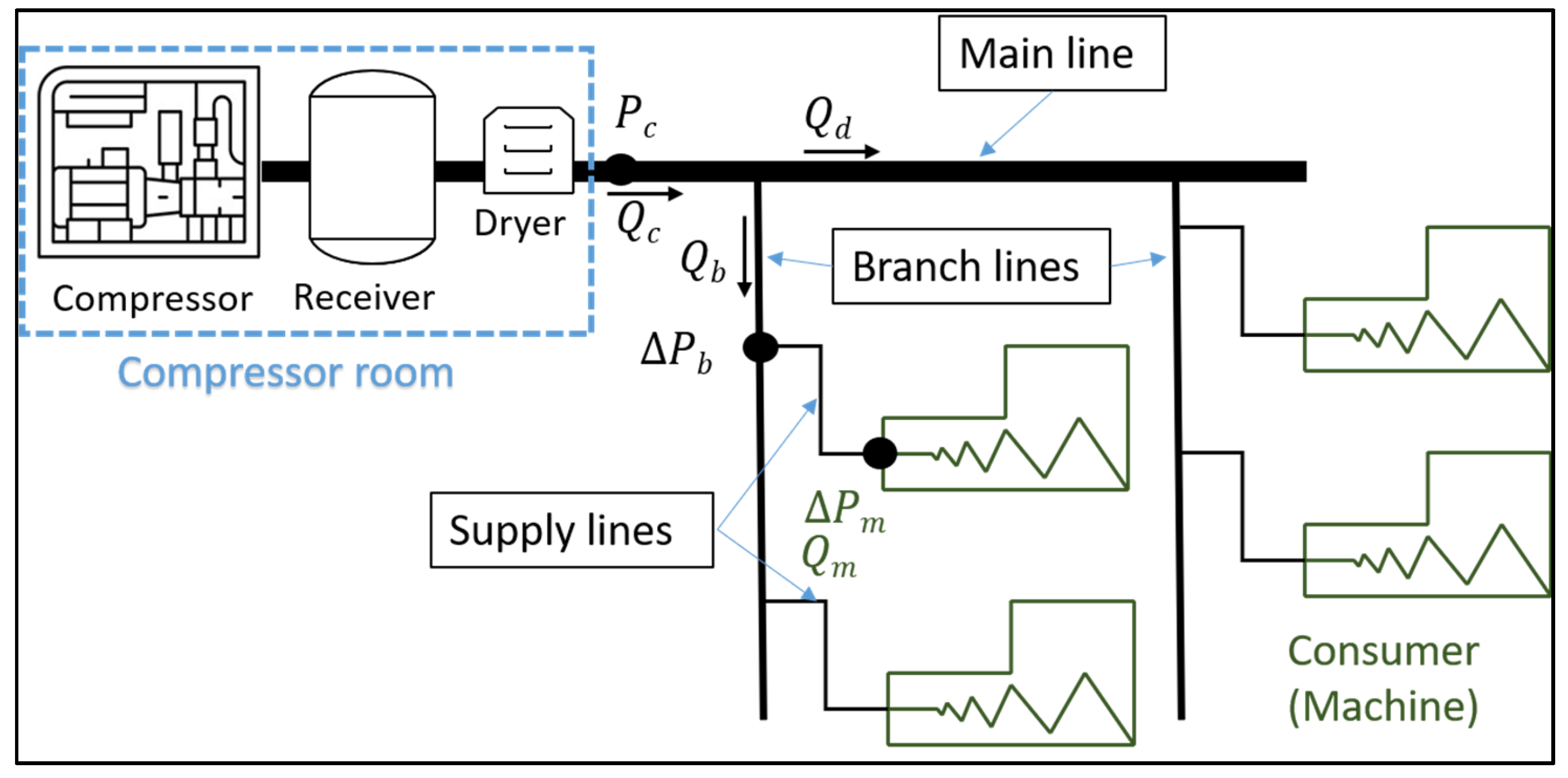
It is essential that the network is designed to avoid pressure drops. The network consists of main lines (mains), branches, and feeder lines (diversions), as shown in Figure 1 [2].
Typically, in pneumatic systems, pipes are made of steel or aluminium, and flexible plastic tubing is also used within the system.
Main lines, which form the shape of the system, are usually pipes with a larger inside diameter. Supply lines connect the main lines or branch lines to the end user (point of use).
Pressure drops or network conductivity depend primarily on three factors: the internal diameters and lengths of the pipes in the main and branch lines (to a minor extent on the pipe material), the layout and shape of the system of main lines and connecting elements, and the type and size of the supply lines.
It is considered best practice to have the main line formed in the form of a closed ring (ring system), but a single main line layout system also has applications (for example, when there is one significantly larger consumer connected directly to the compressor room by a main line with a sufficiently large internal diameter and all other consumers have much smaller consumption) [24].
The pressure at which the system operates has a significant effect on the energy efficiency of compressors. Much research [25,26] shows that, in most cases, the average pressure at the outlet of the compressor room significantly exceeds the pressure required by the end consumers—machines and systems.
In most cases, the reasons for this are a large pressure drop in some parts of the system. This drop is most often caused by inadequate layout of the main lines, branch lines, or supply lines, which forces facility managers or operators to increase the pressure of the compressors, and additional air consumption is generated—the so-called “artificial consumption”.
The pressure drops lead to the following:
-
Up to 20% energy loss [27,28];
-
Reducing the speed and power of actuators;
-
Unpredictable production line shutdowns.
Traditional diagnostic methods based on static measurements at single points in time are insufficient for identifying dynamic anomalies. Therefore, diagnostic methods related to the time characteristics of individual parameters and measured quantities in an industrial pneumatic system are increasingly required.
The diagnosis of these conditions is based on analysis of the shape, length, repetition, and frequency components of the time signals of pressure and flow, measured in real time at the input of the end consumer.
Recognizing the causes of pressure drops through real-time diagnostics is becoming increasingly important due to the need for predictive maintenance.
Time series graphs and peak analysis allow for the detection of structural anomalies. This involves plotting reference points and using graph connectivity to localize the cause of pressure deviations [29].
In [30], the researchers use pattern recognition with wavelet transformation in three different scenarios, proving that, through this method, it is possible to extract different features from a pressure time series and identify different events.
In [31], researchers developed a specific model-based approach using digital twins. The problems with system deviation (in this case, the presence of leaks and pressure drops) are reduced to an optimization problem with an objective function—the difference between the expected and measured values is used to combine structural and behavioral indicators of the state of the system.
There are also a number of sensor-based methods for monitoring and diagnosing the condition of pneumatic systems. The use of artificial intelligence based on neural networks is increasingly becoming popular. In [32], neural networks have been shown to be an effective tool in diagnostics. There are some difficulties and limitations, such as pre-processing the data to eliminate noise and the long training of the neural network to identify different conditions.
From all the above, it is clear that the research attention for optimizing the consumption part of industrial pneumatic systems is mainly focused on dealing with the problem of leaks. In this article, we will demonstrate a method for diagnosing the location of unwanted pressure drops based on statistical analysis of time series of flow and pressure measurements at the inlet of end consumers.
A key part of any pneumatic system is the network of pipelines for the delivery and distribution of compressed air from the compressor installation to the various points of use. This process of transporting the energy of the compressed air leads to pressure losses. Pressure losses are the result of friction within the pipe wall, irregularly shaped sections, constrictions, the used connecting elements, filters, dryers, etc.
The pressure drops or the conductivity of the pneumatic network depend primarily on three factors: the internal diameters and length of the pipes in the main and branch lines (to a minor extent on the material of the pipes), the layout of the system of main lines and connecting elements, and the type and size of the supply lines.
The relationship between pressure and power consumption of compressors is given by the following expression [33]:
W p = ρ a G s R T a K e 0 P a + P P a k 1
where
  W p is the power consumption of the compressor with outlet pressure P [ k W / h ];
k = K 1 / K = 0.2857 ;
K = 1.4 (adiabatic exponent);
ρ a is the air density [1.293 kg/m3];
G s is the compressed air flow rate [Nm3/h];
T a is the inlet air temperature [K];
P a is the inlet pressure [absolute, bar];
P is the outlet pressure [bar];
R is the gas constant of air [286.88 J/kg.K];
e 0 is the efficiency coefficient.
Let us find the ratio of differences at two different pressures P H and P L , where P H > P L .
The percentage change in power consumption is as follows [34]:
W p H W p L W p H 100 = P H 0.2857 P L 0.2857 P H 0,2857 1 100  
( P H = P H g a u g e + 1, P L = P L g a u g e + 1 ).
i.e., if the compressor outlet pressure is set at 7.0 bar and is reduced to 6.0 bar, then the expected energy consumption savings in percentage will be
100 × ( 8.0 0.2857 7.0 0.2857 ) / 8.5 0.2857 = 8.36 % .
Given this, it is essential for the energy efficiency of a pneumatic system that the distribution and supply network is designed and maintained in such a way as to avoid unwanted significant pressure drops.
Even in well-designed and well-sized pneumatic systems, over time, changes occur in the number and type of end consumers, changes of location, addition of new branches, etc., which lead to the appearance of unwanted pressure drops.
Most often, this is detected at times when, due to pressure drops, one or more machines or systems begin to incorrectly perform their operating cycles and/or the safety pressure relays at their input do not switch on or turn off during operation.
Finding the causes of pressure drops at the end points of compressed air use is an important task for the company’s maintenance teams. Correct and quick diagnostics and, respectively, quick and effective elimination of the causes, lead to the prevention of accidents and unwanted production downtime.
The aim of this work is to investigate the possibility of diagnosing the causes of pressure drops at the end user by distinguishing the causes in the supply line or in the branch/main lines based on the measurement of flow rate and pressure (time series) at the end machine inlet.

2. Materials and Methods

The distribution network consists of main lines, branch lines, and supply lines (Figure 2).
Typically, pipelines for pneumatic main and branch lines are made from steel or aluminum, and flexible polymer pipes and hoses are used for supply lines to consumers.
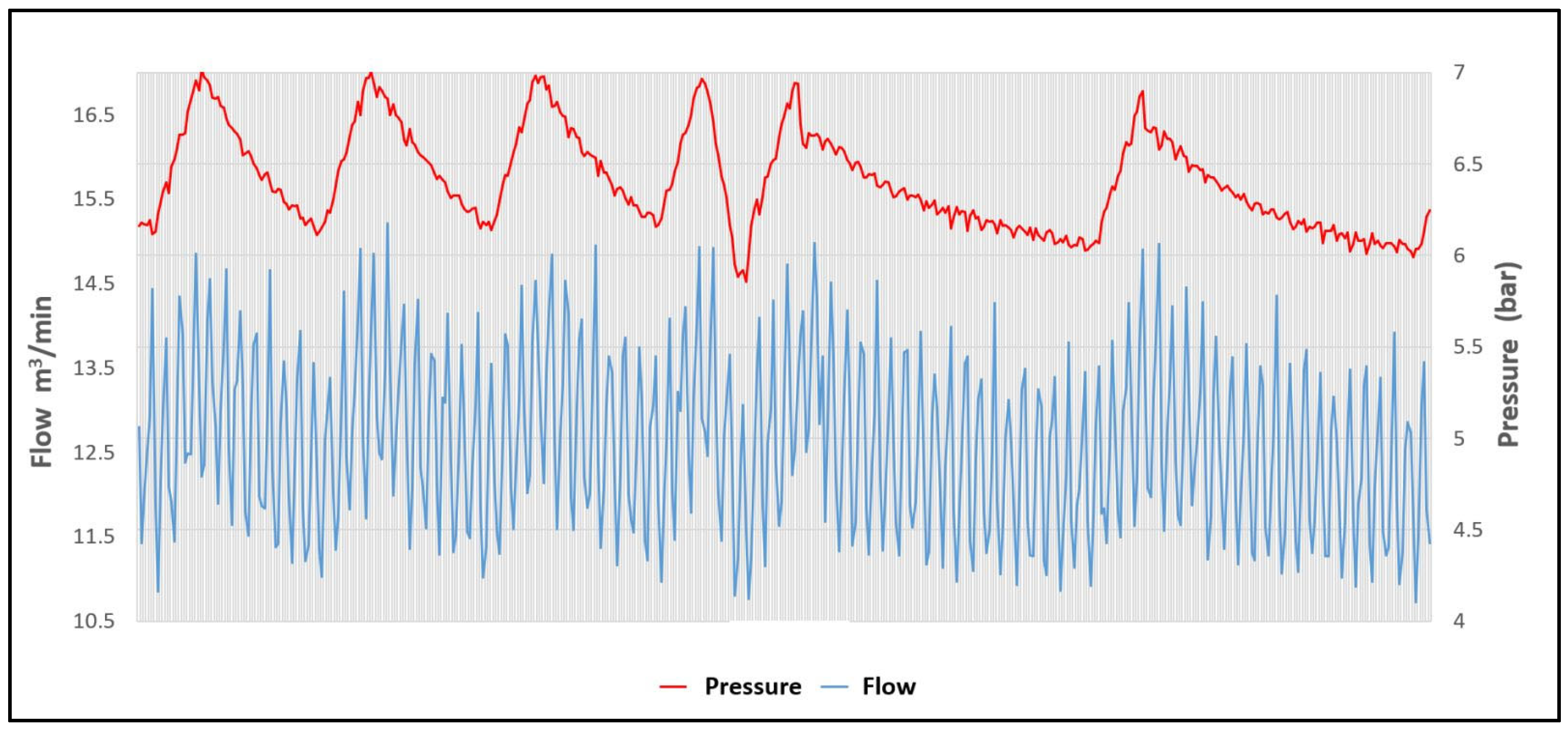
The use of time series diagrams (Figure 3) of measured operating pressure and air consumption is standard practice in the design and maintenance of pneumatic systems.
The compressed air flow profile allows for analyzing the quantitative consumption and compressed air needs in the installation over time and for optimizing the operation of the compressors, especially in the presence of large variations and periods with partial load.
In our case, a compressed air flow meter at the inlet of the end consumer (machine, production line) and a pressure sensor are used, analyzing the correlation between the two time series. In this way, the diagnostic task can be transformed into a time series analysis task.
To calculate the pressure drop in a straight pipe section, the empirical Darcy–Weisbach formula is used [35]:
P = p 1 p 2 = P 1 P 2 = λ L d ω 2 ρ 2
where
P is the pressure drop [Pa] in a pipe with length L[m] and internal diameter d[m];
ω is the average flow velocity [m/s];
ρ is the air density [kg/m3] for certain temperature and atmospheric pressure;
λ is the friction coefficient, depending on the nature of the flow, the Reynolds criterion, and the relative roughness of the inner wall of the pipe;
λ = f ( R e , k e ) ;
R e = ω d p μ ,   k e = d ;
Δ is the equivalent wall roughness.
The literature provides various formulas for calculating λ, but very often, there is a lack of data on the values of the equivalent roughness. Most formulas are derived from experimental studies and represent empirical relationships [36].
Based on many different experimental studies with variations in materials and, respectively, in pipe roughness, different flow profiles, etc., in the literature, we can find several empirical equations giving the dependence of pressure drop ΔP on flow rate QN [37,38,39], which provide sufficiently reliable calculations for practical purposes.
In our study, the following empirical formula was used, giving the relationship between pressure drop and flow rate at the end points of consumption for a flow with subsonic velocity [40,41]:
P m = 7.57 Q 1.85 L 10 4 d 5 P b
where
P m   is the value of the pressure drop at the consumption point (machine) [bar];
Q is the flow rate value at the point of consumption (machine) [m3/min];
P b is the pressure value at the beginning of the supply line [bar].
L is the equivalent length of the supply line [m]. The equivalent length is the sum of the length of the supply line and the equivalent lengths of all connecting elements, valves, and filters along it.
d—internal diameter of the supply line [mm].
In cases where one pipe branches into two or more branches (Figure 2), the pressure drop and flow rate of each part can be calculated as follows:
Q c = Q b + Q d
The pressure drop at any point can be represented as
P b = k b Q c 1.85
P m = P b P m = P c P b P m
For pressure values at the point of consumption,
P m = P c P b 7.57 Q m 1.85 L 10 4 d 5 P c P b .
It follows that the pressure drop at the point of consumption, given a fixed length and diameter of the supply line, is a function of the flow rate to the consumer and the pressure drop at the branch point.

2.1. Correlation Analysis

The most well-known measure in correlation analysis is the Pearson correlation coefficient ( r P e a r s ) [42]. It is applicable to time series such as
r P e a r s = t = 0 N 1 X t X ¯ Y t s Y ¯ t = 0 N 1 X t X 2 t = 0 N 1 Y t s Y ¯ 2
where
X t and Y t are the values of the time series X and Y at time t;
N is the number of points in the time series;
s is the time shift between the two series.
At s = 0, the similarity between time series is assessed without taking into account time shifts.
Since r P e a r s is a measure of linear relationship between time series and does not estimate the difference in time series values, amplitude scaling or translation has no impact on the result.
Pearson’s bivariate correlation is defined by a correlation coefficient (r), which measures the strength and direction of linear relationships between pairs of continuous variables. This correlation is commonly used to measure the following:
-
Correlations between pairs of variables;
-
Correlations within and between sets of variables.
It shows the following:
-
Whether there is a statistically significant relationship between two continuous variables;
-
The strength of the linear relationship (i.e., how close the relationship is to a perfectly straight line);
-
The direction of a linear relationship (increasing or decreasing).
In order to use the Pearson correlation coefficient for reliable analysis, the data to be processed must meet several conditions:
-
Two or more continuous variables;
-
It is not permissible to have missing values for both variables;
-
Linear relationship between variables within the measurement range;
-
Independence of observations. The Pearson bivariate correlation coefficient and the corresponding significance test are not robust when independence is violated.
-
Bivariate normality:
  • Each pair of variables is bivariately normally distributed;
  • Each pair of variables is bivariately normally distributed at all levels of the other variable.
This requirement ensures that the variables are linearly related. Violations of this requirement may indicate that nonlinear relationships exist between the variables. Linearity can be assessed visually using a scatterplot of the data.
The Pearson correlation coefficient takes values in the closed interval [−1, +1]. A value of r X Y = + 1 indicates a functional positive correlation between X and Y, while a value of r X Y = 0   indicates that no correlation can be found (based on the available data and observations) between X and Y. A value of r X Y = 1   indicates a functional inverse relationship between X and Y.
In relation to the range of values of the Pearson correlation coefficient between X and Y, we can distinguish the following cases:
-
r X Y = 1 —the dependent variable Y is perfectly positively correlated with the independent variable X;
-
0.7 r X Y < 1 —this indicates a strong positive correlation of the dependent variable Y with the independent variable X;
-
0.5 r X Y < 0.7 —significant positive correlation of the dependent variable Y with the independent variable X;
-
0.3 r X Y < 0.5 —this indicates a moderate positive correlation of the dependent variable Y with the independent variable X;
-
0 < r X Y < 0.3 —this indicates a weak positive correlation of the dependent variable Y with the independent variable X;
-
r X Y 0 —what is considered the dependent variable Y does not have any kind of linear correlation with what is considered the independent variable X;
-
( 0.3 ) < r X Y < 0 —this indicates a weak negative correlation of the dependent variable Y with the independent variable X;
-
( 0.5 ) < r X Y ( 0.3 ) —this indicates a moderate negative correlation of the dependent variable Y with the independent variable X;
-
( 0.7 ) < r X Y ( 0.5 ) —there is a significant negative correlation of the dependent variable Y with the independent variable X;
-
1 < r X Y ( 0.7 ) —this indicates a strong negative correlation of the dependent variable Y with the independent variable X;
-
r X Y = 1 —the dependent variable Y is perfectly negatively correlated with the independent variable X.
An important question that arises is what is the value of r X Y for which the correlation between variables X and Y can be considered strong or, in any case, satisfactory.
The answer to this question depends on the nature of the problem under consideration, and usual approach is to define this threshold in the phase of the experimental result analysis. Since the proposed approach to examine the location of pressure drop occurrence is new and there is not enough research data on the topic, for now, we will use as an indication of a sufficiently strong correlation between the time series of measured pressure and flow rate the value that is often given in statistical analyzes −0.7. Moreover, for the physical sciences (for example), there should be no doubt about the high degree of correlation between the two variables, so a value of r X Y = 0.7 is considered a reliable threshold of dependence [43].

2.2. Diagnostic Criteria

-
A sign of a problem.
The calculation of exergy flow and accumulated exergy for individual pneumatic components in [44] allowed the analysis of transient processes in them. This analysis revealed that the components act as pneumatic resistors, causing an inevitable pressure drop under dynamic operating conditions.
In other words, the pressure measurement at the inlet of a consumer will show deviations from the maximum value. That is, there will always be a certain pressure drop detected during dynamic processes in a pneumatic consumer.
In scientific articles and technical guidelines and instructions, different values of acceptable pressure drop levels between the main receiver and the final point of use are found—from 3% to 10% [45,46,47,48]. And if there is a consensus that a system in which the pressure drop is greater than 10% is unacceptable, there is no consensus on the lower limit. In our study, we have chosen a pressure drop of 5% as the criterion that determines whether there is a problem or not. The algorithm could work with any level, depending on the goals and the real situation in a given industrial enterprise:
P m m a x P c 100 > 5 % .
-
Indication of the problem being related to the supply line:
r P m Q m 0.7
-
A sign of a structural or systemic problem in the design or implementation of the supply line—excessively large maximum theoretical pressure drop:
P T m a x P c 100 > 5 % .
P T m a x is the maximum theoretically calculated pressure drop.
Based on these criteria, we can define the following groups of cases:
  • P m m a x P c 100 5 %
The pressure drops in the system are within the desired limits.
2.
P m m a x P c 100 > 5 % ; r P m Q m > 0.7
Pressure drops are most likely caused by problems in the main line and/or branch lines, not in the supply line.
3.
P m m a x P c 100 > 5 % ; r P m Q m 0.7 ; P T m a x P c 100 > 5 % .
Since the theoretically calculated pressure drop is significant, this indicates a structural problem in the supply line—small internal diameter and/or long length of the pipes, too many bends, and others due to incorrect design. If r P m Q m 0.7 , there may also be problems in the main and branch lines. In this case, the irregularities in the supply line must first be eliminated, and a new measurement must be made.
4.
P m m a x P c 100 > 5 % ; r P m Q m 0.7 ; P T m a x P c 100 5 % .
In this case, the problem is in the supply line. Changes and deviations from the design documentation have occurred—such as a reduction in the internal diameter of the pipes due to blockages, bends, or kinks, blockage of filters and/or other elements, which leads to incorrect calculation of the equivalent pipe length L, significant leaks in the supply line, and others.

3. Experimental Part

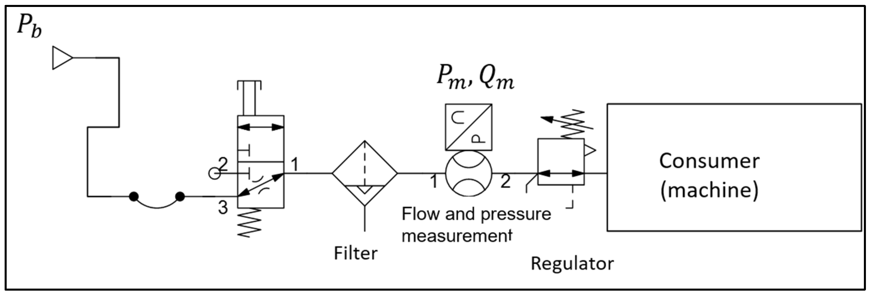
The experimental data represent load diagrams of the instantaneous values of flow rate and inlet pressure (Figure 4) in four plants with different types of production.
The sampling frequency is 1 Hz.
All data were collected from 16 automatic lines in normal production mode in 4 factories with a high degree of automation in Bulgaria. A pressure sensor from the Japanese company SMC–ISE20A was used to measure the pressure (Figure 5).
Some of the sensor characteristics important for measurement purposes are given in Table 1.
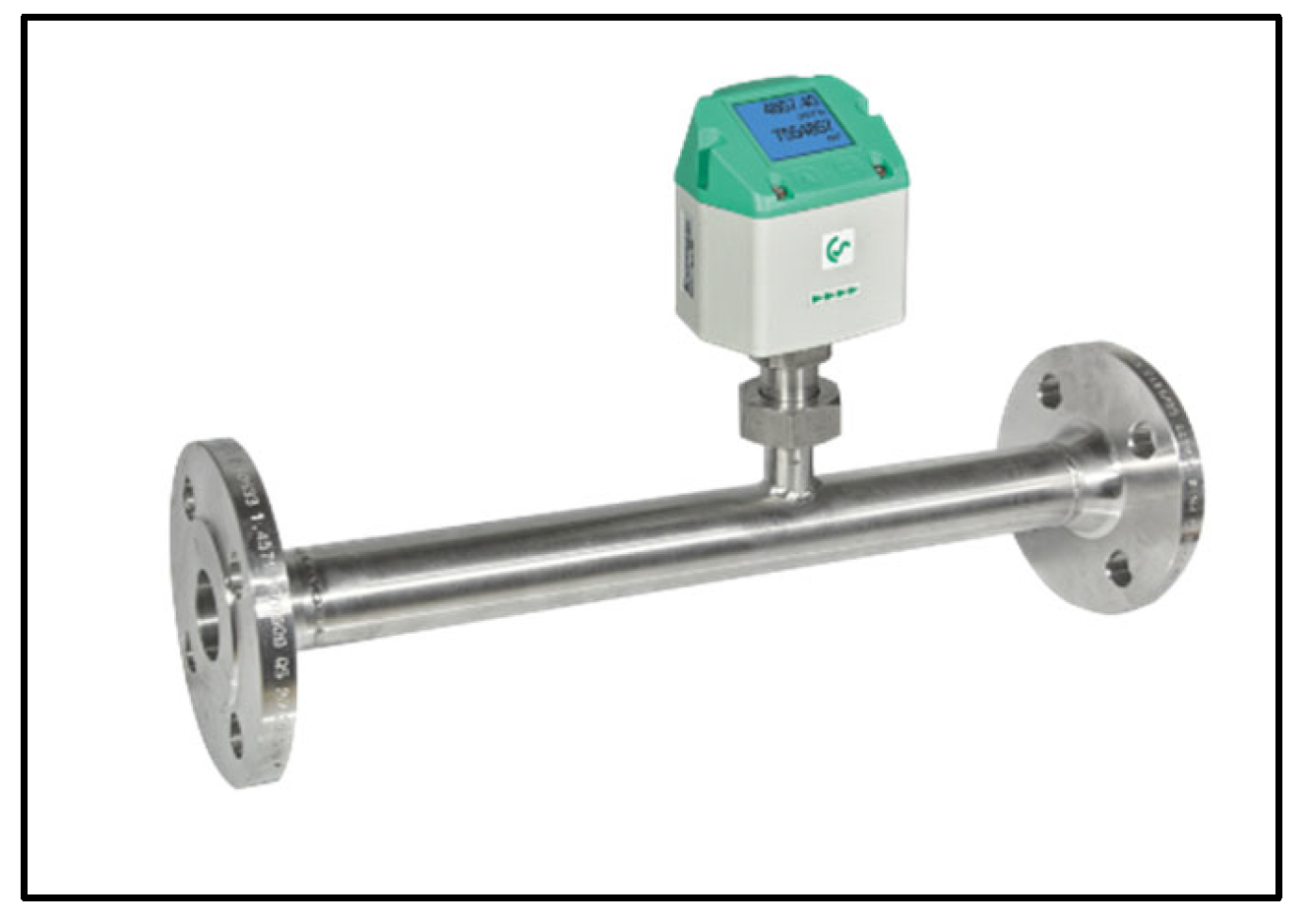
To measure the compressed air flow rate at the inlet of each consumer, CS Instruments (Germany) flow rate sensors from the VA 520 series were used in two modifications: standard and max (Figure 6). The characteristics of the sensors are given in Table 2.
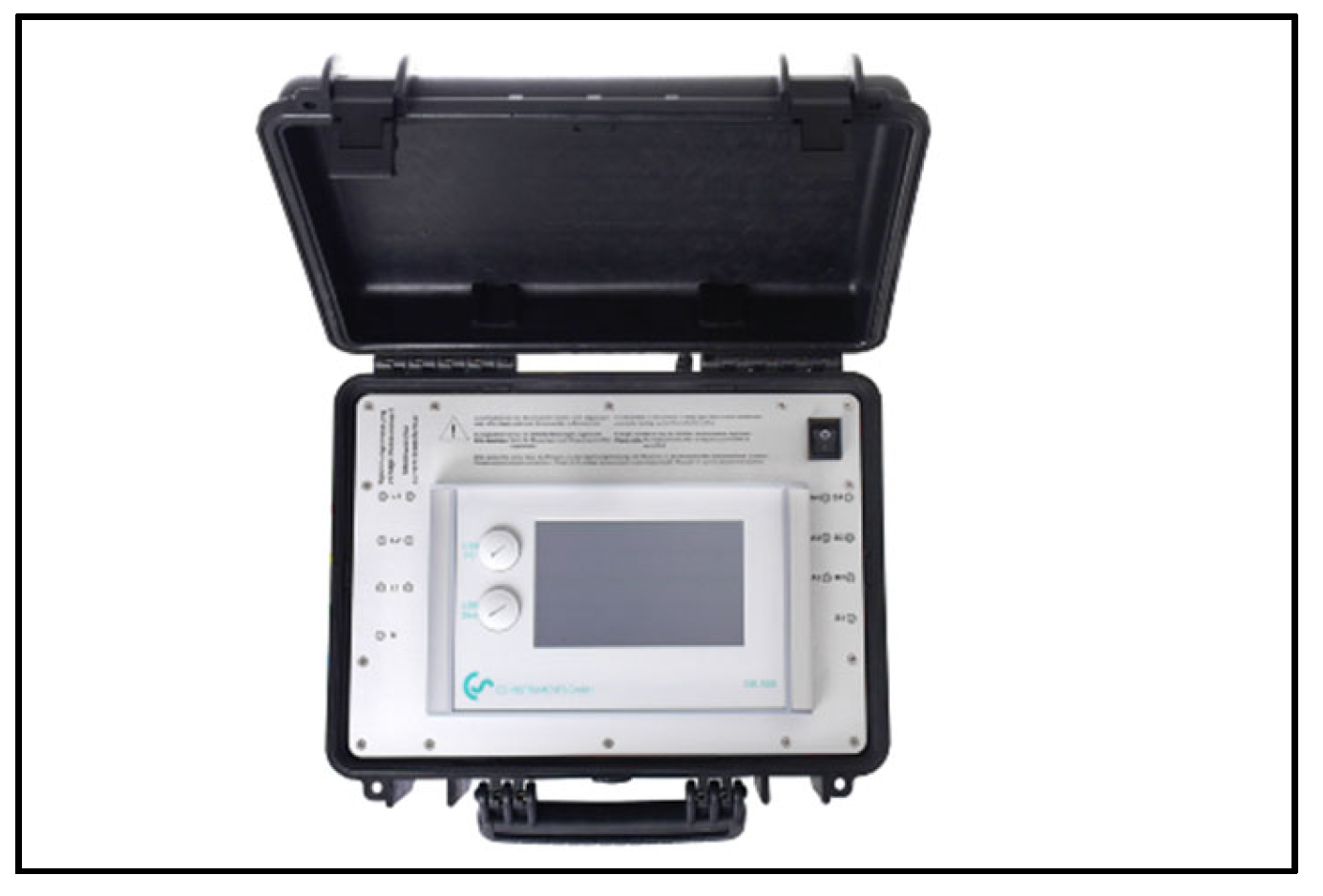
A portable, self-powered data logger from CS Instruments—DS500 Mobile (Figure 7)—was used to collect and record the data.
The accuracy, sampling rate, and other data for the DS 500 Mobile logger are presented in Table 3.
Descriptions of the productions, machines, and initial conditions are given in Table 4. Information on the internal diameter d of the supply lines (in millimeters) and their equivalent length L (in meters) is also available.
The experimental data were recorded as time series of instantaneous flow and inlet pressure values of 16 different machines. The sampling frequency was 1 Hz.
The data were recorded at different time intervals for the different machines, from a few minutes to a few hours, in order to register the different possible states of the machines and lines under study. For example, fully loaded in automatic mode, loaded in semi-automatic mode (where available), machine in production mode but paused, machine at rest but supplied with air, etc.
These data were used for a more complete diagnosis of the condition of the machines’ pneumatic systems.
Since, in some of the machine states—such as rest, stopped from production, pause, setup, semi-automatic or manual mode—the compressed air consumption is not high and pressure drops caused by the machine’s operation are not expected, for the purposes of diagnostics using correlation analysis, data from time periods in which the machine/line was in production mode with maximum load were processed.
In order to calculate theoretical pressure drop ( P T ) for the flow rate time diagrams of each machine, we applied Equation (8) at P b = 0 . This calculated time series gives us the theoretical dependence of P m on   Q m with sufficient reliability. This is verified by the coefficient of determination r P Q between P T   and Q m , as well as for P m and Q m .

4. Results and Analyses

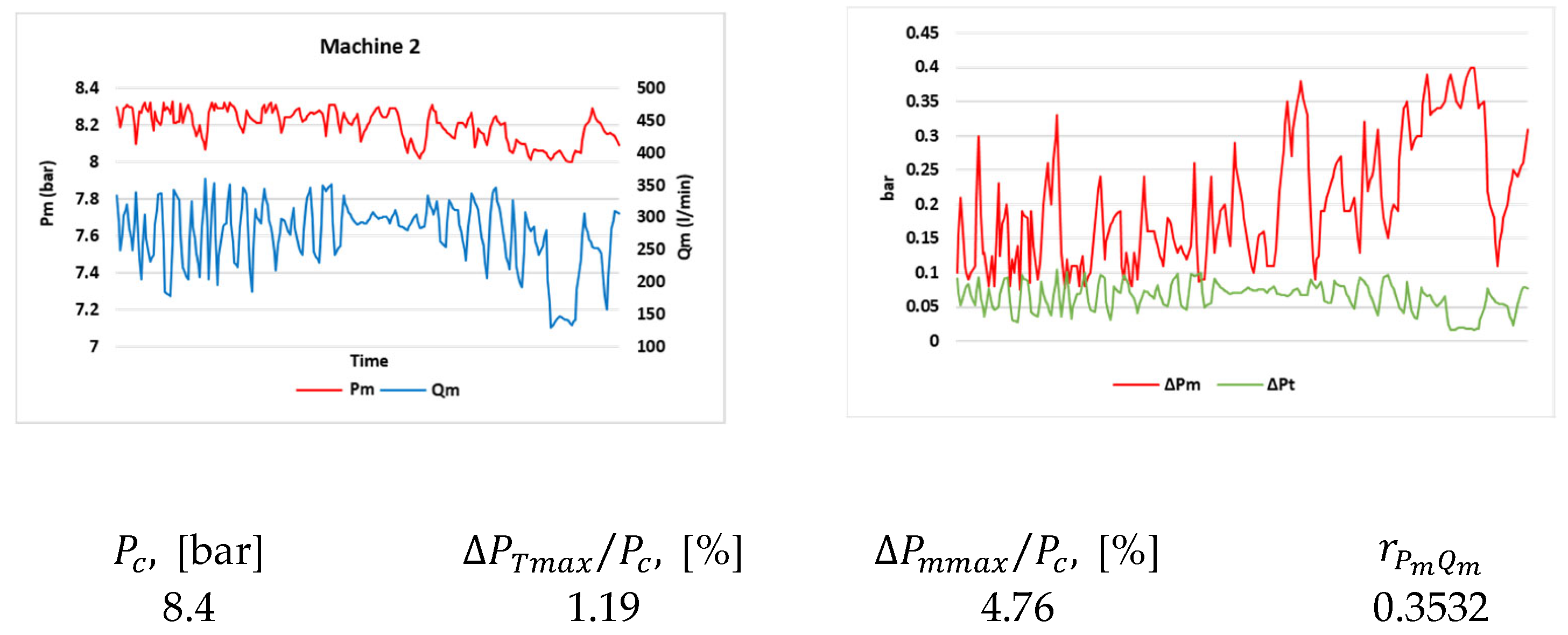
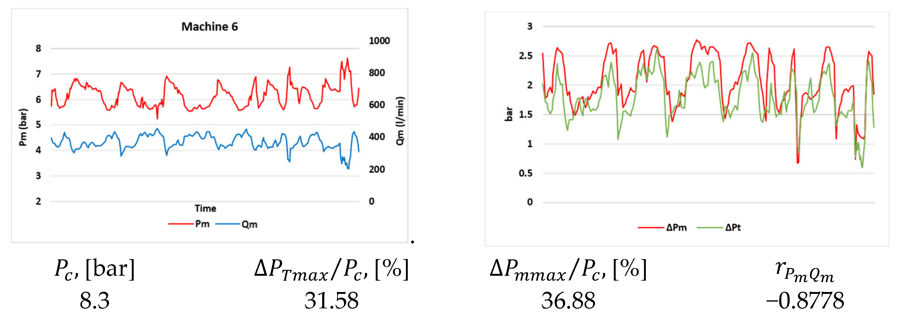
Figure 8, Figure 9, Figure 10 and Figure 11 graphically present the results of four measurements of flow rate ( Q m ) and pressure ( P m ) at the inlet of a consumer at the corresponding P c . The corresponding variables are as follows: P T , defined by (8) at P b = 0 ; r P m Q m , the Pearson correlation coefficient between P m and Q m ; the maximum measured pressure drop; P m m a x = P c P m m i n ;   a n d   P T m a x = P c P T m i n , the maximum pressure drop, determined analytically.

5. Discussion

The data of all 16 machines are given in Table 5.
Figure 12 shows the process of classifying machines according to the described criteria.
In Machines 2 and 4 (Group 1), no pressure drops beyond the desired limits are observed.
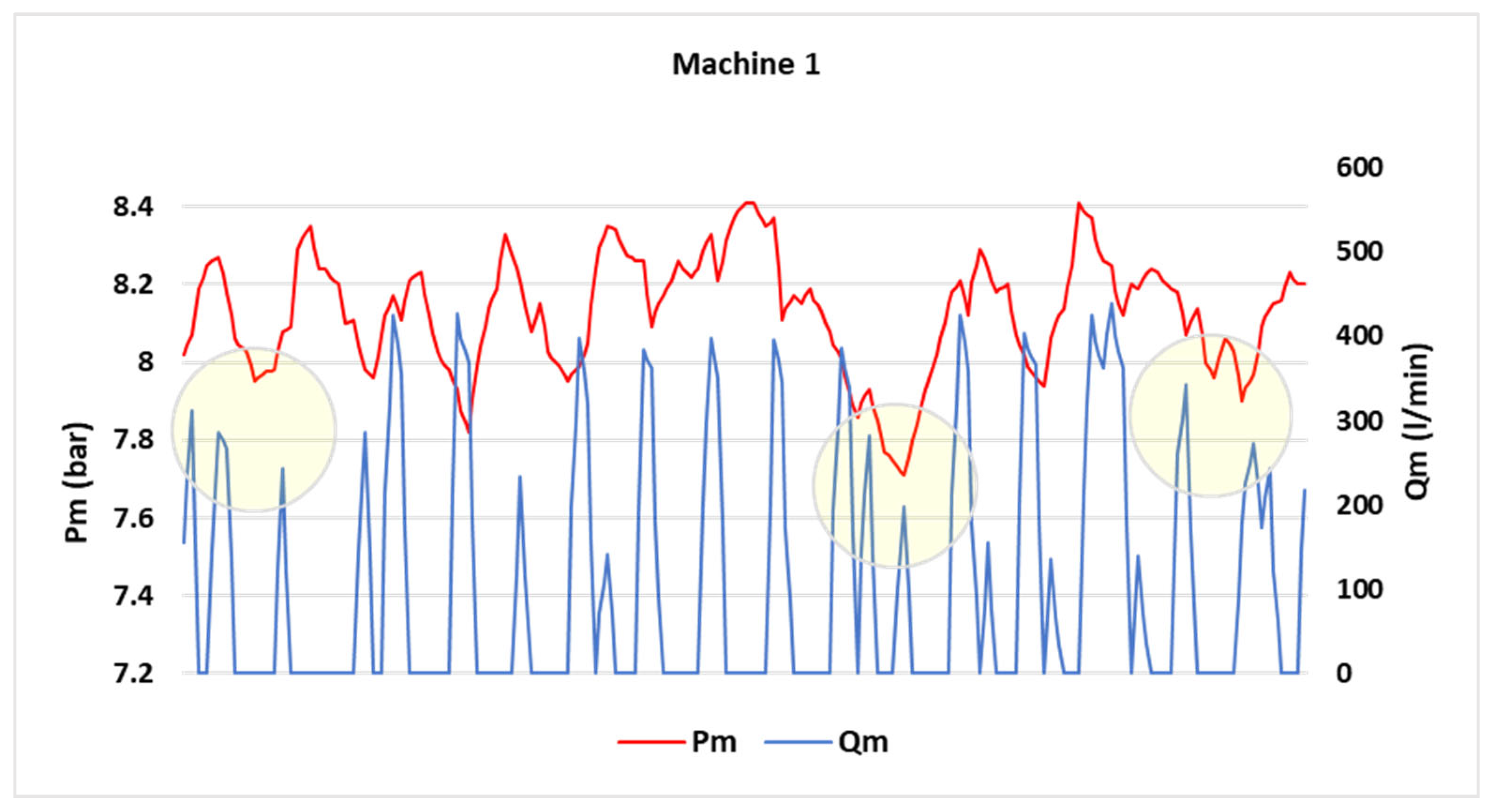
Of the remaining machines, in Machines 1, 3, 8, 9, 14, and 15 (Group 2), the pressure drops were caused by problems outside the supply line, most likely in the mains or branch lines.
In the remaining Machines, 5, 6, 7, 10, 11, 12, 13, and 16, the pressure drops are caused by problems in the supply line. These machines are classified into two groups.
Machines 6, 10, 11, and 13 fall into Group 3, where the pressure drops are due to a problem in the design and/or execution of the supply line.
Machines 5, 7, 12, and 16 fall into the final group, Group 4, where pressure drops are due to problems in the supply line caused by changes in the line during operation—blockages, kinks, leaks, etc.
The experimental data were collected from 16 machines in four different plants in Bulgaria. The report with the results was submitted to the plant management in order to take action to eliminate the causes of the unwanted pressure drops and to test the proposed diagnostic method.
So far, only the “Automobile hydraulic pump plant” has taken action:
Machine 10: Press–supply line—replacing the 8 mm inner diameter supply hose with a 13 mm (1/2”) inner diameter flexible hose.
Machine 11: Press–supply line—replacing the 8 mm inner diameter supply hose with a 13 mm (1/2”) inner diameter flexible hose, eliminating a leak in the supply line tap.
Machine 12: Automatic assembly—the 8 mm inner diameter supply hose with a 13 mm (1/2”) inner diameter flexible hose, removing a large leak in the supply line manual valve.
Machine 13: Automatic assembly and test in clean room—the 8 mm inner diameter supply hose with a 13 mm (1/2”) inner diameter flexible hose.
The results of the measures taken is given in Table 6.
Machines 10 to 13 fell into Groups 3 and 4 according to the classifier problems with the supply line.
In Machine 11, the cause of the large pressure drop turned out to be not only the incorrectly sized initial supply line (according to the classifier, the machine falls into Group 3), but also, there was a leak in the manual valve at the connection between the supply line and the branch line.
The presence of a large leak in the supply line of Machine 12 was predicted by the proposed classification method.
In most plants, there is no established practice of mapping the pressure in the main lines, respectively, placing pressure sensors in the main lines and branch lines. In the plants we studied, the situation is the same; therefore, we cannot confirm the results of the classifier with data from the corresponding sensors. We can make a visual analysis of the graphs of the synchronized time series of pressure and flow of machines falling into category 2.
In the marked sections (Figure 13), unusual pressure drops are observed at low or even zero consumption, which, in theory, according to Equation (8), is possible only if ∆Pb is different from 0. That is, we have a pressure drop at the inlet of the supply line, which is generated somewhere else in the system of main and branch lines.
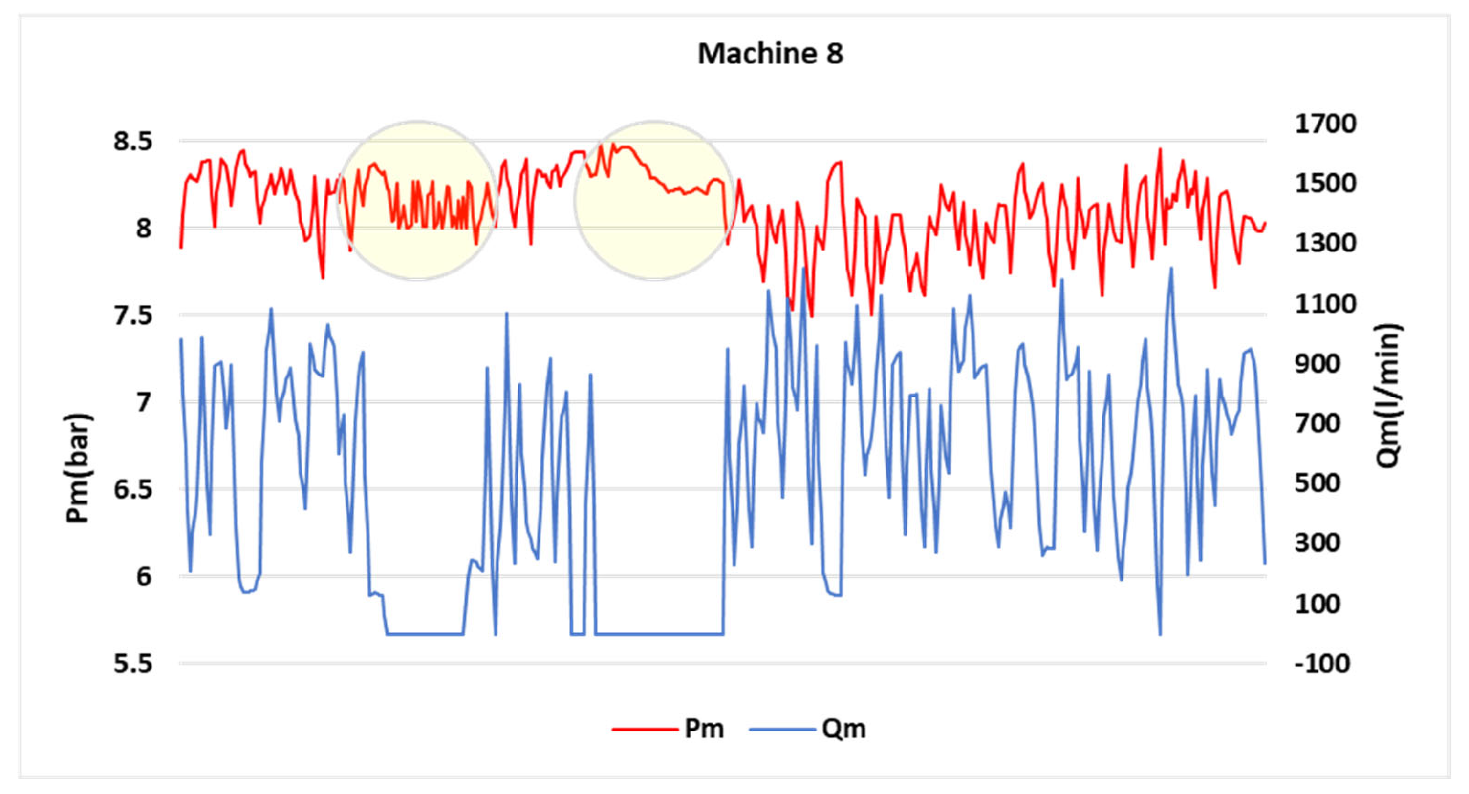
The situation is similar to Machine 8 (Figure 14).
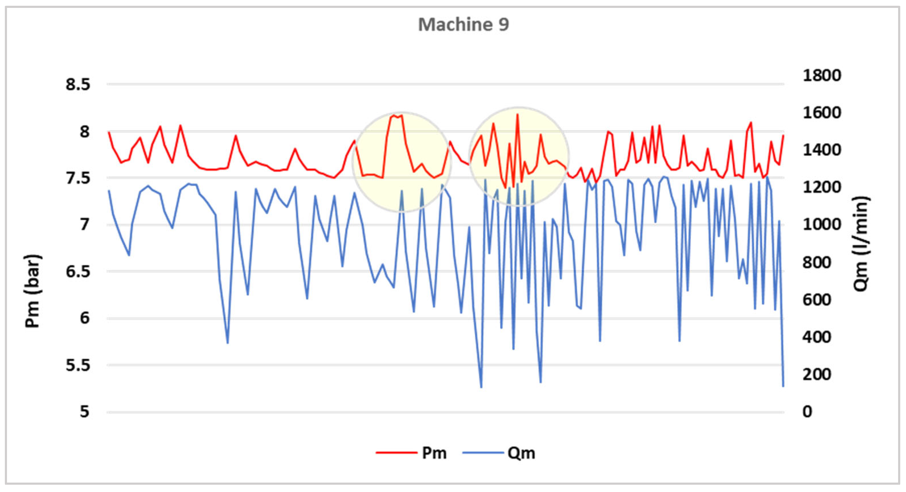
In Machine 9 (Figure 15), another type of anomaly is observed. Peaks of relatively high-pressure values occur in moments with high air flow. At the same time, the pressure drop relative to the receiver pressure is large—reaching up to 1 bar.
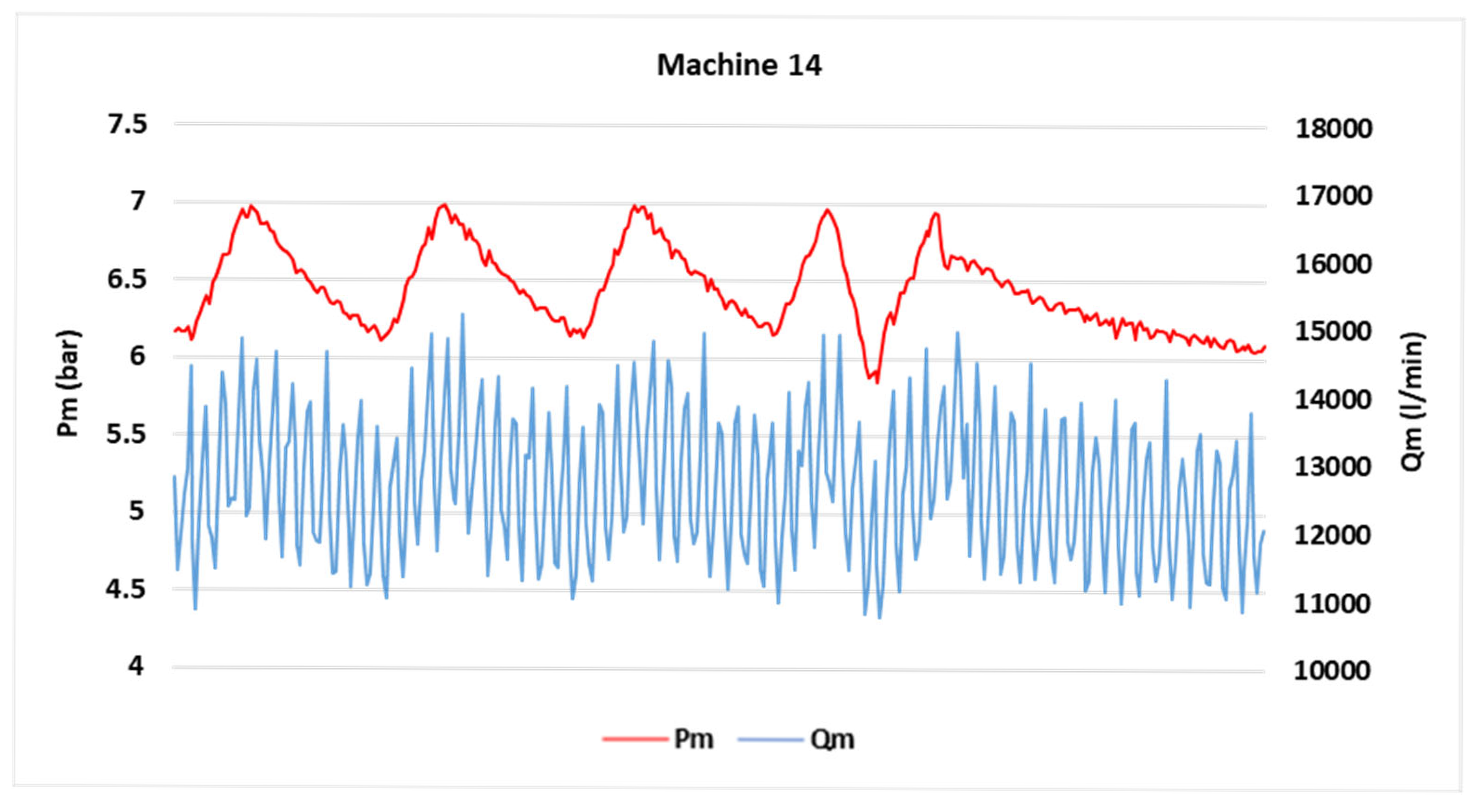
In Machine 14 (Figure 16), how the flow rate exactly follows the shape of the inlet pressure is visible. That is, the large pressure drops are formed before the supply line, most likely by a larger consumer nearby and supplied by the same branch line.
Visual inspection of data from some of the machines also confirms the conclusions drawn based on the proposed classifier.
Conclusions from the discussion of the results are as follows:
-
The Pearson correlation coefficient between flow rate and end-user inlet pressure is a promising indicator for distinguishing whether pressure drop is due to supply line problems. This was confirmed both by actual troubleshooting of supply line problems on Machines 11 to 13 and by visual analysis of time diagrams on machines falling into Group 2. More real-world data are needed to empirically determine its threshold value more definitively;
-
Using the theoretical maximum pressure drop to separate the causes of problems in the supply line has practical application, but it requires additional knowledge of the supply line itself, and its parameters must be included in the calculations. From a practical point of view, it turns out that it is better for machines classified in Groups 3 and 4 to inspect the entire supply line and, if there are kinks, blockages, or leaks, to eliminate them. And, if after that, the pressure drop is still above the permissible level, optimize the internal diameter and length of the supply line;
-
The higher correlation coefficient above the specified threshold does not mean that the problem is only in the supply line. For example, in Machines 11 and 12, after eliminating the problems in the supply line, the pressure drop is still high, although within the specified permissible limits. However, searching for the causes of pressure drops in the main and branch lines is a significantly more complex task, often associated with stopping entire production sections. The proposed method can solve the problem to some extent without the need for unnecessary pressure increase in the compressor and the generation of artificial consumption.

6. Conclusions

The problem of unwanted pressure drops is one of the main ones in compressed air distribution. Diagnosing the causes of these drops is a laborious task, which is also associated with stopping the entire production with all the losses as a consequence. To compensate for the drops that have occurred, an unjustified increase in pressure in the compressor installations is often resorted to, which leads to significant energy losses and the spread of the negative effect on other elements of the system.
In modern production systems, increasing attention is paid to optimizing energy flows. For this purpose, monitoring systems are implemented that monitor and analyze the consumption of the main energy carriers. Compressed air is also monitored. In addition to the total flow rate of the production unit and the pressure in the compressor room, in more detailed monitoring systems, the flow rate and pressure of individual consumers are measured in real time for the purpose of energy monitoring.
To overcome the difficulties in detecting the causes of pressure drops in compressed air transmission and distribution systems, this article proposes an approach for diagnostics of pneumatic systems based on the monitoring of load diagrams and indicators obtained based on the model principle for fault detection. An analysis of experimentally collected data from 16 production machines and lines was performed. The data were collected based on a passive experiment on actual, functioning production systems in leading manufacturing companies. Due to the confidential nature of the information, the companies are not mentioned.
Assessments of criteria are presented, by which it is possible to establish the causes of unwanted pressure drops. In this case, drops in the supply lines and their elements or systemic ones—in the main and branch structure and the compressor installation.
The developed diagnostic algorithm could easily be incorporated into industrial energy monitoring software environments, which could diagnose the problem in real time and provide guidance for its solution.

Author Contributions

Conceptualization, T.T. and R.K.; methodology, T.T. and R.K.; validation, R.K.; formal analysis, T.T.; investigation, R.K.; resources, R.K.; data curation, T.T.; writing—original draft preparation, T.T.; writing—review and editing, R.K.; visualization, R.K. All authors have read and agreed to the published version of the manuscript.

Funding

This research was funded by the European Regional Development Fund within the OP “Research, Innovation and Digitalization Programme for Intelligent Transformation 2021–2027”, Project No. BG16RFPR002-1.014-0005 Center of competence “Smart Mechatronics, Eco- and Energy Saving Systems and Technologies”.

Data Availability Statement

The data presented in this study are available on request from the corresponding author due to confidentiality of corporate data about problems in production facilities.

Conflicts of Interest

The authors declare no conflict of interest.

References

  1. Blaustein, E.; Radgen, P. Compressed Air Systems in the European Union; LOG_X Verlag GmbH: Stuttgart, Germany, 2001. [Google Scholar]
  2. Kosturkov, R.; Nachev, V.; Titova, T. System Analysis and Opportunities for Optimization of Pneumatic Systems in Manufacturing Plants. TEM J. 2019, 8, 749–763. [Google Scholar] [CrossRef]
  3. Werner, K.; Löbbe, S.; Büttner, S.; Schneider, C. Establishing Energy Efficiency—Drivers for Energy Efficiency in German Manufacturing Small- and Medium-Sized Enterprises. Energies 2020, 13, 5144. [Google Scholar] [CrossRef]
  4. Nehler, T.; Parra, R.; Thollander, P. Implementation of energy efficiency measures in compressed air systems: Barriers, drivers and non-energy benefits. Energy Effic. 2018, 11, 1281–1302. [Google Scholar] [CrossRef]
  5. Ge, Z.; Song, Z.; Ding, S.X.; Biao, H. Data Mining and Analytics in the Process Industry: The Role of Machine Learning. IEEE Access 2017, 5, 20590–20616. [Google Scholar] [CrossRef]
  6. Ge, Z. Review on data-driven modeling and monitoring for plant-wide industrial processes. Chemom. Intell. Lab. Syst. 2017, 171, 16–25. [Google Scholar] [CrossRef]
  7. Cesarotti, V.; Orazi, S.D.; Introna, V. Improve Energy Efficiency in Manufacturing Plants through Consumption Forecasting and Real Time Control: Case Study from the Pharmaceutical Sector. In Proceedings of the International Conference on Advances in Production Management Systems (APMS 2010), Cernobbio, Italy, 11–13 October 2010. [Google Scholar]
  8. Qi, G.; Zhu, Z.; Erqinhu, K.; Chen, Y.; Chai, Y.; Sun, J. Fault-diagnosis for reciprocating compressors using big data and machine learning. Simul. Model. Pract. Theory 2018, 80, 104–127. [Google Scholar] [CrossRef]
  9. Magoulès, F.; Zhao, H.-X. Data Mining and Machine Learning in Building Energy Analysis; John Wiley & Sons: Hoboken, NJ, USA, 2016. [Google Scholar] [CrossRef]
  10. Tran Yes, T.; Chen, Y.; Chau, M.Q.; Ning, B. A robust online fault detection and diagnosis strategy of centrifugal chiller systems for building energy efficiency. Energy Build. 2015, 108, 441–453. [Google Scholar] [CrossRef]
  11. Xiao, F.; Zheng, C.; Wang, S. A fault detection and diagnosis strategy with enhanced sensitivity for centrifugal chillers. Appl. Therm. Eng. 2011, 31, 3963–3970. [Google Scholar] [CrossRef]
  12. López, A.J.G.; Márquez, A.C.; Macchi, M.; Fernández, J.F.G. Prognostics and Health Management in Advanced Maintenance Systems. In Advanced Maintenance Modeling for Asset Management; Springer: Cham, Switzerland, 2018; pp. 79–106. [Google Scholar] [CrossRef]
  13. Xenos, D.P.; Cicciotti, M.; Kopanos, G.M.; Bouaswaig, A.E.; Kahrs, O.; Martinez-Botas, R.; Thornhill, N.F. Optimization of a network of compressors in parallel: Real Time Optimization (RTO) of compressors in chemical plants—An industrial case study. Appl. Energy 2015, 144, 51–63. [Google Scholar] [CrossRef]
  14. Lee, J.; Kao, H.-A.; Yang, S. Service Innovation and Smart Analytics for Industry 4.0 and Big Data Environment. Procedia CIRP 2014, 16, 3–8. [Google Scholar] [CrossRef]
  15. Benedetti, M.; Cesarotti, V.; Introna, V. From energy targets setting to energy-aware operations control and back: An advanced methodology for energy efficient manufacturing. J. Clean. Prod. 2017, 167, 1518–1533. [Google Scholar] [CrossRef]
  16. Zhang, K.; Peng, K.; Chu, R.; Dong, J. Implementing multivariate statistics-based process monitoring: A comparison of basic data modeling approaches. Neurocomputing 2018, 290, 172–184. [Google Scholar] [CrossRef]
  17. Xiao, W. A probabilistic machine learning approach to detect industrial plant faults. Int. J. Progn. Health Manag. 2016, 7. [Google Scholar] [CrossRef]
  18. Benedetti, M.; Bonfà, F.; Introna, V.; Santolamazza, A. Real Time Energy Performance Control for Industrial Compressed Air Systems: Methodology and Applications. Energies 2019, 12, 3935. [Google Scholar] [CrossRef]
  19. Semitela, Â.; Silva, J.; Girão, A.F.; Verdasca, S.; Futre, R.; Lau, N. Combining Infrared Thermography with Computer Vision Towards Automatic Detection and Localization of Air Leaks. Sensors 2025, 25, 3272. [Google Scholar] [CrossRef]
  20. Boyko, V.; Weber, J. Cycle Time-Based Fault Detection and Localization in Pneumatic Drive Systems. Actuators 2024, 13, 447. [Google Scholar] [CrossRef]
  21. Kosturkov, R.; Nachev, V.; Titova, T. Expert estimation of leakage in the pneumatic systems in the bottling industry. IOP Conf. Ser. Mater. Sci. Eng. 2020, 878, 012008. [Google Scholar] [CrossRef]
  22. Motazedi, N.; Beck, S. Leak detection using cepstrum of cross-correlation of transient pressure wave signals. Proc. Inst. Mech. Eng. Part C J. Mech. Eng. Sci. 2017, 232, 2723–2735. [Google Scholar] [CrossRef]
  23. Kosturkov, R.; Titova, T.; Nachev, V. Diagnosis of Pneumatic Systems on the Basis of Time Series and Generalized Feature for Comparison with Standards for Normal Working Condition. TEM J. 2021, 10, 183–191. [Google Scholar] [CrossRef]
  24. Paramonov, A.; Starikov, A. Air Supply Systems for Enterprises; Lan: Moskow, Russia, 2011; Available online: https://elima.ru/books/?id=1752 (accessed on 12 January 2025). (In Russian)
  25. Silva, W.L.V.; Souza, L.C.O.; Bortolaia, L.A.; de Paula, M.R.; Leal, E.M. Study of the electricity consumption reduction of a compressed air system: The case of a steelmaking company. REM—Int. Eng. J. 2017, 70, 421–428. [Google Scholar] [CrossRef]
  26. Unger, M.; Radgen, P. Energy Efficiency in Compressed Air Systems: A review of energy efficiency potentials, technological development, energy policy actions and future importance. In Proceedings of the 10th International Conference on Energy Efficiency in Motor Driven Systems (EEMODS’2017), International Con-ference on Energy Efficiency in Motor Driven Systems EEMODS, Rome, Italy, 6–8 September 2017; Bertoldi, P., Ed.; Publications Office of the European Union: Luxembourg, 2018; pp. 207–233. [Google Scholar]
  27. Dindorf, R.; Wos, P. Automatic measurement system for determination of leakage flow rate in compressed air pipeline system. Metrol. Meas. Syst. 2018, 25, 59–70. [Google Scholar] [CrossRef]
  28. Eret, P.; Harris, C.; O’Donnell, G.; Meskell, C. A practical approach to investigating energy consumption of industrial compressed air systems. Proc. Inst. Mech. Eng. Part A J. Power Energy 2012, 226, 28–36. [Google Scholar] [CrossRef]
  29. Harman, A.; Baur, L.; Wolf, C.; Sauer, A. Detection of Anomalies in Compressed Air Systems using Time of Occurrence and KPI Analysis. In Proceedings of the 5th International Conference on Communications, Information, Electronic and Energy Systems (CIEES), Veliko Tarnovo, Bulgaria, 20–22 November 2024. [Google Scholar] [CrossRef]
  30. Thabet, M.; Sanders, D.A.; Bausch, N. Detection of Patterns in Pressure Signal of Compressed Air System Using Wavelet Transform. In Energy and Sustainable Futures, Proceedings of the 2nd ICESF 2020, Hatfield, UK, 10–11 September 2020; Springer: Cham, Switzerland, 2021; pp. 61–67. [Google Scholar] [CrossRef]
  31. Travaš, V.; Gal, E.; Lučin, I.; Žic, E. Digital twin for a real-time leakage detection and localization in pressurized piping systems. J. Hydroinformatics 2025, 27, 755–770. [Google Scholar] [CrossRef]
  32. Tiboni, M.; Remino, C. Condition Monitoring of Pneumatic Drive Systems Based on the AI Method Feed-Forward Backpropagation Neural Network. Sensors 2024, 24, 1783. [Google Scholar] [CrossRef] [PubMed]
  33. Mueller, J.; Boyle, W.C.; Popel, I.H.J. Aeration: Principles and Practice, 1st ed.; CRC Press: Boca Raton, FL, USA, 2002; Volume 11. [Google Scholar] [CrossRef]
  34. Kissock, K.; Schmidt, C. Modeling and Simulation of Air Compressor Energy Use. ACEEE Summer Study Energy Effic. Ind. 2005, 1, 131–142. [Google Scholar]
  35. Perevoshchikov, S.I. Design and Operation of Compressor Stations; TyumGNTU: Tyumen, Russia, 1996; ISBN 5-88465-034-5. [Google Scholar]
  36. Popov, G.; Nikolov, G.; Boyadzhiev, M.; Klimentov, K. Investigation of errors in calculating friction coefficients in round pipes, Yearbook of the University of Mining and Geology “St. Ivan Rilski”, 2010, Volume 53, is. I. pp. 159–162. Available online: https://mgu.bg/wp-content/uploads/2025/05/Vol.-53-I-2010-159-162.pdf (accessed on 15 January 2025). (In Bulgarian).
  37. Barenblatt, G.I.; Chorin, A.; Prostokishin, V. Scaling Laws for Fully Developed Turbulent Flow in Pipes: Discussion of Experimental Data. Proc. Natl. Acad. Sci. USA 1997, 94, 773–776. [Google Scholar] [CrossRef] [PubMed]
  38. Marcus, R.D.; Leung, L.S.; Klinzing, G.E.; Rizk, F. Single Phase Flow in Pneumatic Conveying Systems of Solids; Springer: Dordrecht, The Netherlands, 1990. [Google Scholar]
  39. SMC Corporation. Energy Saving Manual. SMC Corporation: Tokyo, Japan, 2013. [Google Scholar]
  40. Engineering ToolBox, Compressed Air—Pressure Loss in Pipe Lines—Online Calculator with Metric and Imperial Units. Available online: https://www.engineeringtoolbox.com/pressure-drop-compressed-air-pipes-d_852.html (accessed on 1 November 2020).
  41. Atlas Copco. Atlas Copco Air Compendium; Atlas Sopco AB: Stockholm, Sweden, 1975. [Google Scholar]
  42. Rodgers, J.L.; Nicewander, W.A. Thirteen Ways to Look at the Correlation Coefficient. In The American Statistician; American Statistical Association: Alexandria, VA, USA, 1988; pp. 59–66. [Google Scholar]
  43. Hahs-Vaughn, D. Foundational methods: Descriptive statistics: Bivariate and multivariate data (correlations, associations). In International Encyclopedia of Education; Elsevier: Amsterdam, The Netherlands, 2023; pp. 734–750. [Google Scholar] [CrossRef]
  44. Rakova, E.; Weber, J. Process simulation of energy behaviour of pneumatic drives. Procedia Eng. 2015, 106, 149–157. [Google Scholar] [CrossRef]
  45. Taylor, B. What Is Compressed Air Pressure Drop and How Do You Minimize It. Fluid-Aire Dynamics Ltd. 21 September 2021. Available online: https://fluidairedynamics.com/blogs/articles/what-is-pressure-drop-and-how-its-costing-you-money#:~:text=An%20efficient%20compressed%20air%20system%20should%20lose,not%20receive%20enough%20pressure%20to%20operate%20correctly (accessed on 10 June 2025).
  46. Hernandez-Herrera, H.; Silva-Ortega, J.I.; Martínez Diaz, V.L.; Sanchez, Z.G.; García, G.G.; Escorcia, S.M.; Zarate, H.E. Energy Savings Measures in Compressed Air Systems. Int. J. Energy Econ. Policy 2020, 10, 414–422. [Google Scholar] [CrossRef]
  47. Oster, C. Detecting and Minimizing Air Pressure Drop in Compressed Air Systems. JHFOSTER Ltd. 2 April 2025. Available online: https://jhfoster.com/automation-blogs/what-is-a-pressure-drop-and-how-do-you-prevent-it/ (accessed on 10 June 2025).
  48. Taylor, B. Air Compressor Troubleshooting: Pressure Problems. Fluid-Aire Dynamics, 4 July 2023. Available online: https://fluidairedynamics.com/blogs/articles/air-compressor-troubleshooting-pressure-problems (accessed on 10 June 2025).
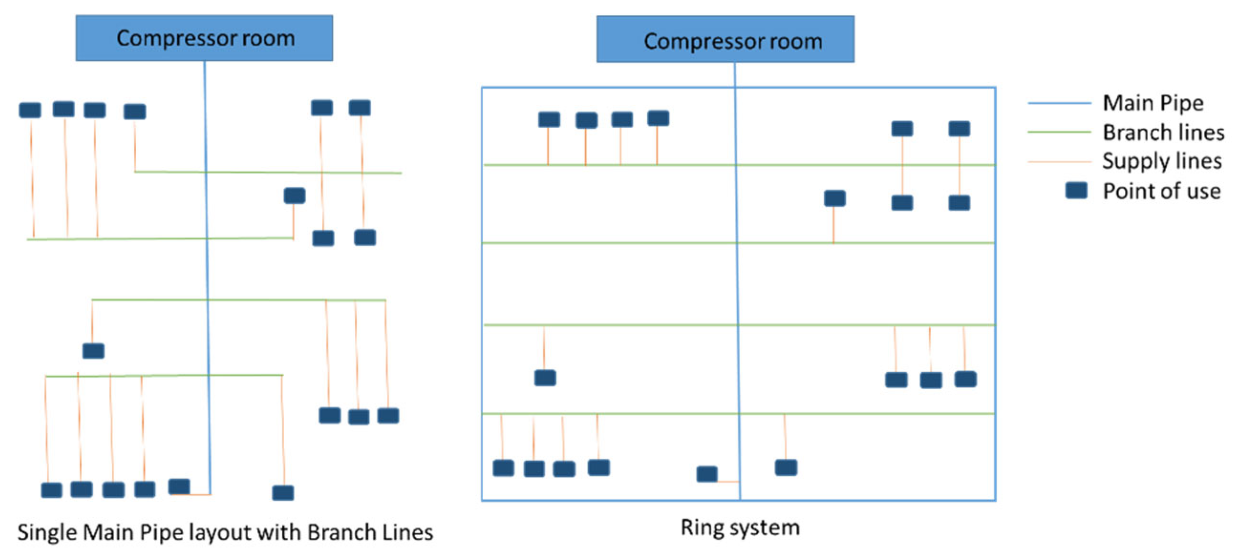
Figure 1. Two types of compressed air distribution systems [2].
Applsci 15 09536 g001
Figure 2. Typical distribution network.
Applsci 15 09536 g002
Figure 3. Flow and pressure time series.
Applsci 15 09536 g003
Figure 4. Experimental setup.
Applsci 15 09536 g004
Figure 5. Multifunction programmable pressure sensor SMC ISE20A.
Applsci 15 09536 g005
Figure 6. CS Instruments VA520 flowmeter with flange connection.
Applsci 15 09536 g006
Figure 7. CS Instruments DS 500 Mobile data logger.
Applsci 15 09536 g007
Figure 8. Machine 2. Load diagram of flow rate Q m , pressure P m , pressure drop P m , and the theoretically calculated pressure drop P T .
Applsci 15 09536 g008
Figure 9. Machine 3. Load diagram of flow rate Q m , pressure P m , pressure drop P m , and the theoretically calculated pressure drop P T .
Applsci 15 09536 g009
Figure 10. Machine 5. Load diagram of flow rate Q m , pressure P m , pressure drop P m , and the theoretically calculated pressure drop P T .
Applsci 15 09536 g010
Figure 11. Machine 6. Load diagram of flow rate Q m , pressure P m , pressure drop P m , and the theoretically calculated pressure drop P T .
Applsci 15 09536 g011
Figure 12. Classifying machines according to the described criteria.
Applsci 15 09536 g012
Figure 13. Machine 1. Load diagram of flow rate Q m and pressure P m .
Applsci 15 09536 g013
Figure 14. Machine 8. Load diagram of flow rate Q m and pressure P m .
Applsci 15 09536 g014
Figure 15. Machine 9. Load diagram of flow rate Q m and pressure P m .
Applsci 15 09536 g015
Figure 16. Machine 14. Load diagram of flow rate Q m and pressure P m .
Applsci 15 09536 g016
Table 1. Characteristics of SMC ISE 20A pressure sensor.
ModelSMC ISE20A
FluidApplicable fluidCompressed air, non-flammable gases, non-corrosive gases
Temperature range0 to 50 °C
PressureMeasurement range−0.100 to 1.000 MPa
AccuracyRepeatability±0.2% FS
Analog output±2.5% FS (ambient temperature: 25 ± 3 °C)
Analog output linearity±1% FS
Analog
Output
TypeCurrent output: 4 to 20 mA
Response time1.5 ms or less
Table 2. Characteristics of the CS VA 520 standard/max flow meter.
ModelCS VA 520 StandardCS VA520 Max
FluidApplicable fluidCompressed air, N2; quality: ISO 8573-1 1.1.2 to 1.6.2.
Temperature range−30 to 80 °C
Measurement methodThermal, in-line
Fluid velocity92.7 m/s185 m/s
PressureNominal working pressure−0.1 to 1.6 MPa
AccuracyRepeatability±1.5% of the measured value ± 0.3% FS
Analog
output
TypeCurrent output: 4–20 mA
Response timeMinimum: 0.05 s.
Digital outputRS 485 interface (Modbus-RTU), Ethernet, M-Bus
Table 3. CS DS500 Mobile data logger features.
ModelCS Instruments DS 500 Mobile
Sensor inputsUp to 12 sensor inputs—digital or analog. Programmable Digital CS sensors for dew-point measurement with SDI interface. Flow sensors on CS. Other sensors with RS 485/Modbus RTU. Analog CS sensors for pressure, flow, temperature, etc. Other analog sensors with outputs 0/4–20 mA, 0–1/10/30 V, pulse outputs Pt100/Pt1000, and KTY.
Input signalsCurrent signal (0–20 mA/4–20 mA) and internal or external power supplyMeasurement range0–20 mA/4–20 mA
Resolution0.0001 mA
Accuracy±0.03 mA ±0.05%
Input resistance50 Ω
Sampling
frequency
10 ms, 100 Hz
Non-volatile memory4 GB
Table 4. Descriptions of the productions, machines, and initial conditions.
MachinePressure
P c
Equivalent Length of the Supply Line Inner Diameter of the Supply Line d
[bar][m][mm]
Flexible water connection plantMachine 1- Sealant application8.496
Machine 2—Sealant application8.4810
Machine 3—Automatic shear8.5610
Machine 4—Pressing and molding8.4716
Machine 5—Cutting and sorting8.52.58
Electronic components factoryMachine 6—Automatic soldering8.3106
Machine 7—Assembly unit8.41210
Machine 8—Robotic assembly8.5512
Machine 9—Robotic assembly8.4512
Automobile hydraulic pump plantMachine 10—Press6.73.58
Machine 11—Press6.84.58
Machine 12—Automatic assembly6.81010
Machine 13—Automatic assembly and test in clean room5.7510
Household plastic products factoryMachine 14—Blast line7.3550
Machine 15—Sorting and arranging7.31520
Machine 16—Packaging machine7.338
Table 5. Summary results of machine measurements.
Machine[bar] P T m a x / P c P m m a x / P c r P m Q m
[%][%]
Machine 18.42.02%8.33%−0.0431
Machine 28.41.19%4.76%0.3532
Machine 38.52.12%16.00%−0.3900
Machine 48.41.43%4.76%−0.2768
Machine 58.53.60%16.59%−0.9508
Machine 68.331.58%36.88%−0.8778
Machine 78.43.38%9.40%−0.7046
Machine 88.52.92%11.41%−0.4175
Machine 98.42.98%11.90%0.1652
Machine 106.716.17%17.91%−0.9046
Machine 116.814.19%23.09%−0.8759
Machine 126.84.42%21.76%−0.7293
Machine 135.75.11%5.79%−0.9321
Machine 147.30.34%19.81%0.3742
Machine 157.32.35%23.56%−0.3939
Machine 167.34.18%29.59%−0.8461
Table 6. Results of the measures.
Initial StateAfter Correction
PCEquivalent Length of the Supply Line LInner Diameter of the Supply Line d∆Pmmax∆Pmmax/PcEquivalent Length of the Supply Line LInner Diameter of the Supply Line d∆Pmmax∆Pmmax/Pc
[bar][m][mm][bar][%][m][mm][bar][%]
Machine 106.7581.217.91%5130.22.99%
Machine 116.84.581.5723.09%5130.34.41%
Machine 126.810101.4821.76%10130.34.41%
Machine 135.75100.335.79%5130.11.75%
Disclaimer/Publisher’s Note: The statements, opinions and data contained in all publications are solely those of the individual author(s) and contributor(s) and not of MDPI and/or the editor(s). MDPI and/or the editor(s) disclaim responsibility for any injury to people or property resulting from any ideas, methods, instructions or products referred to in the content.