A Case Study on Virtual HPC Container Clusters and Machine Learning Applications

Abstract

This article delves into the innovative application of Docker containers as High-Performance-Computing (HPC) environments, presenting the construction and operational efficiency of virtual container clusters. The study primarily focused on the integration of Docker technology in HPC, evaluating its feasibility and performance implications. A portion of the research was devoted to developing a virtual container cluster using Docker. Although the first Docker-enabled HPC studies date back several years, the approach remains highly relevant today, as modern AI-driven science demands portable, reproducible software stacks that can be deployed across heterogeneous, accelerator-rich clusters. Furthermore, the article explores the development of advanced distributed applications, with a special emphasis on Machine Learning (ML) algorithms. Key findings of the study include the successful implementation and operation of a Docker-based cluster. Additionally, the study successfully showcases a Python application using ML for anomaly detection in system logs, highlighting its effective execution in a virtual cluster. This research not only contributes to the understanding of Docker’s potential in distributed environments but also opens avenues for future explorations in the field of containerized HPC solutions and their applications in different areas.

1. Introduction

Early computers were large, expensive to build, and had limited computational power. Initially, they were used for long and tedious calculations and were not part of the consumer market, accessible only to select government or academic organizations. The advent of minicomputers, despite their smaller size, did not immediately solve these issues, due to their still-high cost and limited capabilities. The technological breakthrough came with the miniaturization of devices and the development of high-speed local computer networks, which led to a significant reduction in the cost of electronic devices, making computers more accessible to the general public. This miniaturization also enabled the installation of multiple processors on a motherboard, leading to the development of supercomputers with hundreds or even thousands of processors. This advancement was significant because it coincided with growing interest in parallel algorithms, which divide larger tasks into smaller parts to be executed by multiple processors simultaneously. The physical limitations of processors and the inefficiency of overclocking due to heat generation led to a focus on multiprocessing and multi-core processors.

Next, computational clusters, extending the concept of multiprocessing, created extensive parallel or distributed systems, offering vast computational power. Instead of investing in a single high-performance device, the idea is to network many units with less powerful but cheaper components, often virtualized to achieve a more cost-effective overall performance. Simultaneously, containerization has emerged as a solution to software portability issues. This technique involves combining an application with its dependencies into an image, which is then run on an isolated container, making the application independent of the specific computer platform and facilitating its distribution and deployment.

Today, the goal is to build a virtual computational container cluster using containerization on the Docker platform. It was therefore essential to validate the cluster’s functionality, evaluate its performance, and demonstrate a practical application. This article covers the following:

(1)

Preparation of Dockerfile scripts for building images to launch a cluster on the Docker platform, including the installation of the Message Passing Interface (MPI) communication standard and the configuration of containers for distributed programs.

(2)

Development and a use of a distributed application using Machine Learning (ML), demonstrating the effects of parallel processing on computation time in a containerized structure.

Our study focuses on the intersection of Docker and High-Performance Computing (HPC), exploring how Docker’s containerization technology can be leveraged to enhance the performance and scalability of HPC systems. Kononowicz and Czarnul [1] performed a detailed performance assessment of Docker-based MPI applications, demonstrating minimal overhead. Zervas et al. [2] and Zhou and Georgiou [3] explored a Slurm–Kubernetes orchestration, running HPC workloads under Kubernetes environments. Kuity and Peddoju [4] further investigated container performance metrics on ×86 and OpenPOWER systems. We delve into the practical implications of this integration, particularly in the realm of ML for anomaly detection in system logs, a domain that has seen limited exploration in the existing literature. This research aims to close the gap between the theoretical potential and practical application of Docker in HPC environments, providing valuable insights and contributions to this emerging field [5].

The article is divided into the following sections: Section 2 provides a comprehensive overview of the evolution and significance of computational clusters, detailing their transition from exclusive use in government and academic organizations to more widespread accessibility, due to technological advancements like miniaturization and the development of high-speed local computer networks. Section 3 contains a brief exposition of the system architecture used in this research, including details on the Docker environment, the configuration of the virtual HPC clusters, and the implementation of ML algorithms. This section gives the technical specifics and methodologies employed in the ML applications, particularly focusing on the use of Long Short-Term Memory (LSTM) networks for anomaly detection, along with detailed descriptions of the data transformation and neural network training processes. Section 4 discusses the real-world performance and application of the models and systems described, providing empirical data and analysis to showcase the efficacy of the proposed methods. Finally, Section 5 provides a comprehensive summary and the conclusions of the findings, along with implications for future research in this field.

2. Related Work

Here, we delve into existing research on Docker’s application in HPC and machine learning. This section provides a comprehensive background and highlights the research gap addressed in this study. Early attempts to enable containers on high-performance-computing systems showed that plain Docker images could be transplanted to user-privilege runtimes such as Singularity without harming MPI scalability or GUI-driven engineering workflows. Kumar et al. [6] converted Docker images to both Singularity and Sarus and, on an InfiniBand cloud cluster, observed performance differences within the noise of native NAS benchmarks and an OpenFOAM GUI run. Their study is now the baseline for ‘native-like’ performance against which newer, more automated systems are judged.

2.1. Docker in HPC

Before containerization became firmly established in the field of computer system administration as a new technique for creating segregated environments with varied software stacks, traditional virtualization, also known as hardware-level virtualization, was the prevailing method. The roles of virtual machines and containers are similar in many areas, leading to the natural assumption that there might have been attempts to prepare an artificial cluster using the former method. Indeed, there are scientific works discussing how to do this [7,8,9].

Sergeev et al. [10] explored the stability and reliability of Docker containers running on Windows operating systems under resource-deficit conditions. Their work, focusing on stress and volume testing, was crucial for understanding the performance of Docker containers under extreme load conditions, a relevant aspect when considering the efficiency of virtual HPC clusters. The authors [11] discussed the application of Zero Trust principles to Docker containers, proposing the Zero Trust Container Architecture. This framework is particularly relevant for ensuring security in containerized environments, an aspect that complements this study’s focus on Docker in HPC. Zhang et al. [12] presented a neural network approach for recommending suitable base images for Docker containers, a key aspect in optimizing container performance and efficiency. Their work aligns with this study’s interest in enhancing Docker container performance in HPC environments.

Traditional virtualization never gained sufficient popularity in real HPC clusters, although it was considered due to its potential use in providing supercomputers as multi-user systems [13]. Since containerization has often been compared with traditional virtualization, studies have emerged comparing the performance of both techniques [14], including analyses of their application in HPC systems [15,16]. Tests were conducted using the Kernel-based Virtual Machine hypervisor and the Docker containerization platform. They evaluated computational performance, the performance of data-intensive applications, network communication efficiency depending on network topology, and memory usage. Generally, the results favored the use of containerization over virtual machines to achieve the highest efficiency. However, Docker is not without flaws. The performance of default-configured containers is primarily degraded by Docker’s layered file system and the Network Address Translation used in network communication, although the negative effects of both mechanisms can be mitigated [14]. A significant downside of both virtualization techniques is the increased overhead on input–output operations [14], especially those performed on local resources shared with many systems, such as hard drives and bridged network interfaces. However, the overhead on CPU usage is negligible, regardless of the chosen technique [17].

Over recent years, hardware virtualization has only improved in performance [18], thanks to the widespread adoption of supporting technologies such as the Intel VT and AMD-V series. Although traditional virtualization remains irreplaceable in many areas of computing (e.g., leased private virtual servers), it was containerization and its promised ‘lightness’ (in terms of computer resource load) that effectively encouraged those interested in HPC to conduct experiments and discover practical applications of containers in HPC systems, leading to the emergence of dedicated containerization platforms, such as Shifter [19].

Given the current state of technology, using traditional virtualization to prepare an artificial computational cluster is also questionable. The purpose of such a cluster is not necessarily to gain high computational power, but to provide a special environment for comfortably programming parallel applications, testing them, and generally becoming familiar with the functioning of a cluster, without the need to have access to a real supercomputer. The problem with virtual machines lies more in the complexity of their configuration, difficulties in managing them, and potentially in how much they burden computer resources (CPU, memory, disk space). By analyzing instructions for launching a cluster with virtual machines [8,9], it was found that the presented installation and configuration process seemed time-consuming and prone to errors.

The earliest attempt to create a virtual cluster on Docker containers was most likely documented in a 2014 paper [13], around the time of the rapid rise in popularity of this technology. Containers allow for the delivery of varied software stacks (including selected Linux distributions and MPI implementations) according to user needs, simplifying the administration of HPC systems, as there is no need to compromise on globally installed dependencies. The goal of the work was to demonstrate that Docker performs well in HPC clusters based on the MPI standard and InfiniBand communication interfaces. However, the proposal in [13] more closely resembles a concept and does not present a practical way of implementing a virtual cluster [20].

Soon after, descriptions of practical methods for building a virtual cluster on Docker containers appeared. The authors of [21] aimed to solve the issue of different user preferences regarding dependencies installed in the cluster system, which led to problems related to the stability of the operating system and software portability. They designed the architecture of a virtual cluster to allocate isolated environments on a physical cluster, each containing specific dependencies and individually assigned to users. Such a configured virtual cluster is characterized by ease of scalability, as expanding it only requires the addition of more containers. Unfortunately, no performance tests of the containerized cluster were conducted in the work [21]. The authors also did not mention the standard Docker Compose tool, which would greatly simplify the reproduction and management of the virtual cluster on a local machine, not to mention other container orchestration platforms essential for managing the overall infrastructure (e.g., Docker Swarm, Kubernetes).

Building on earlier ideas [13,21], the paper in [22] refined the method of containerizing a cluster using Docker. Compared to previous proposals, this approach seems to be the most user-friendly. It was recognized that too much time is spent on installing and configuring the system, network, development tools, and dependencies before programming and deploying MPI applications. Therefore, a ready-to-use environment was prepared, where programmers could immediately start their work, including writing code and building and testing MPI-based programs. Container orchestration was entrusted to the integrated Docker Swarm platform. With its help, several physical machines with Docker services were connected into a network. Docker Swarm automatically balanced the load by distributing containers among physical nodes. The virtual cluster in the work [22] was not subjected to performance tests. Additionally, the proposal offers a rather limited set of configuration options.

While Docker has been successful in the area of cloud and internet technologies and often forms an integral part of microservice architectures, over time it has been found that it does not meet the requirements of many production HPC environments [23,24]. Among the distinctive features of this platform that hinder its application in supercomputers are the lack of native mechanisms for user authentication, authorization, and accounting; its dependence on disk space; and isolation from host resources [24]. Also problematic is Docker’s use of the cgroups subsystem, which imposes top-down limitations on the use of computer resources, while in HPC environments, it is usually the queue system (e.g., SLURM) that primarily manages this  [19]. In response to Docker’s shortcomings, alternative containerization platforms dedicated to deployment in HPC systems have been developed. One such platform is Shifter [19], implemented at the National Energy Research Scientific Computing Center in California. Its users run tasks from their chosen container images (user-defined images, UDIs). Shifter was designed with special attention given to performance and scalability, not only of the applications themselves but also of the installation process of containers and images. It was also intended to provide access to shared resources in containers, including parallel file systems and internal networks. An important feature was the ability to cooperate with queue systems and to support handling images designed for other containerization platforms (including Docker).

In addition to Shifter, there are at least two related containerization platforms: Singularity and Charliecloud. Both of these have been subjected to performance studies [23]. They tested computational, memory, and application performance, as well as RAM usage, based on benchmark tests such as SysBench, STREAM, and HPCG. It turned out that the performance drop caused by containerization was very small or even non-existent. The additional memory demand for each platform was considered minimal. Furthermore, it was found that the implementation of containerization essentially had no impact on performance. Of course, this conclusion only applies to these three platforms dedicated to HPC systems and does not concern Docker. However, it is possible that Docker would perform just as well, assuming that it uses the same isolation techniques as the tested platforms.

For the purposes of this thesis, the solution presented in [22] was the most suitable, where only the possibilities of easily programming parallel applications were mentioned. The work [22] focused more on containerization in production environments, rather than development and testing environments.

Study of the integration of Docker technology in HPC and ML applications intersects with various works in the field. For example, the article [25] focused on TensorFlow, a comprehensive framework for large-scale ML on heterogeneous distributed systems. The content aligns closely with the themes discussed in this article, particularly in the context of utilizing complex computational systems for advanced ML tasks. The authors highlighted TensorFlow’s ability to map computations onto various hardware platforms, thus facilitating both research and deployment of ML models in numerous domains. They underscored TensorFlow’s evolution, emphasizing improvements in performance, flexibility, and support for a broader range of models and hardware. Key aspects covered in the document include model parallel training, where different portions of a model computation are carried out simultaneously on different computational devices, and concurrent steps for model computation pipelining to optimize utilization during the training of deep neural networks. In relation to our research, this document can provide insights into how such virtual HPC clusters could be optimized and utilized for running complex ML models like those implemented in TensorFlow. The parallelization and distribution strategies discussed for TensorFlow are particularly relevant for managing large-scale computations in virtual HPC environments.

2.2. ML for Anomaly Detection

There is a notable gap in studies on implementing ML algorithms in dockerized HPC environments. Such studies could provide valuable insights into the efficiency and scalability benefits of Docker in HPC. Dayo’s study in [26] delved into the deployment of applications using Docker containers and Kubernetes clusters, highlighting the efficiency and scalability offered by these technologies in managing ML workloads. This approach mirrors the themes discussed in this study on virtual HPC clusters, where containerization plays a crucial role in enhancing the performance and manageability of ML applications. In this research, the emphasis is on leveraging the power of virtualization and containerization, as seen with technologies like Docker, to streamline the development and deployment of ML models. This methodology is crucial in handling the large-scale computational demands of ML, particularly in the training and inference phases. Dayo’s exploration of Kubernetes clusters for orchestrating containerized applications further complements this study’s focus on virtual HPC clusters. Kubernetes, being a powerful tool for managing containerized applications at scale, aligns well with the needs of ML workflows, which often require complex coordination of resources and tasks. The aspect of system log analysis in Dayo’s article is particularly relevant in the context of monitoring and optimizing ML applications running on virtual HPC clusters. Effective log analysis can lead to insights into performance, resource utilization, and potential bottlenecks in these complex systems, thus enabling more informed decisions about optimizing computational resources and model parameters.

Roth et al. [27], Deng [28], and Li [29] investigated anomaly detection techniques, which were closely related to this study’s application of ML for anomaly detection in system logs. These works provided insights into the state-of-the-art methods in anomaly detection, an area explored within the Docker-based virtual HPC cluster. Li et al. [30] and Zavrtanik, Kristan, and Skocaj [31] focused on self-supervised learning approaches for anomaly detection and localization. Their findings are particularly relevant for understanding the application of advanced ML techniques in anomaly detection, a key component of this study. The works of Xiao, Rasul, and Vollgraf [32] on the Fashion-MNIST dataset, and Snoek, Larochelle, and Adams [33] on Bayesian optimization of ML algorithms provide foundational knowledge for ML applications, which informs this study’s approach to utilizing ML in Docker environments. Abadi et al. [25] and Ajasa et al. [34] discussed TensorFlow, a framework for large-scale ML on heterogeneous distributed systems. This is particularly relevant to this study’s focus on ML in HPC environments, providing a potential tool for implementing ML algorithms.

Container technology now underpins end-to-end AI/ML pipelines. Scientists are now packaging entire AI/ML workflows in containers. Nandi et al. [35] built a Docker-enabled federated-learning platform where TensorFlow workers and an MQTT broker ran in rootless containers. Experiments on an edge-cloud/HPC test-bed showed near-linear scaling on multimodal physiological streams. González-Abad et al. [36] paired udocker with Horovod to create a cluster-agnostic GPU-training pipeline. Because udocker uses pure user-space Python, it works on several supercomputers without admin help and with parity to native Conda. For production pipelines that frequently rebuild images, Balasubramanian [37] formalized best practices—layer caching, automated smoke tests, and post-run clean-up—that cut cloud costs, while keeping MPI/Slurm integration points intact.

Despite the widespread interest in the subject of ML, there have been no studies describing the use of a containerized cluster to perform these types of calculations. Everyone shows how to set up a cluster in containers in general, but no one presents using it for a real problem, which poses a number of issues. The startup itself is not new, but using it to solve AI/ML problems is.

3. Container Architecture

This part of the article describes the technical framework and setup used for the research. It includes details on the Docker environment and the configuration of the virtual HPC container clusters (Figure 1).

3.1. Container Clusters

The virtual cluster architecture used in this work is based on [22]. A single container constitutes a cluster node. One acts as the supervisory node (designated master), while the others are worker nodes (named worker). The containers are grouped with Docker Compose and connected by an isolated internal network that handles process management and inter-container communication. All containers are launched from the same node image stored locally, differing only in configuration. When the cluster is enabled, the user connects to the supervisory node through a remote-control client or simply attaches to the container shell with Docker. Docker Compose allows the cluster to be started, removed, or scaled with single console commands. Once activated, it is almost immediately ready for use, so the user may begin programming and testing applications. Cluster nodes are automatically discovered by a script in the supervisory container; their addresses are written to a hosts file in a predefined location, eliminating manual preparation.

Two basic types of images were distinguished. The base image provides only the selected MPI implementation, which has been previously compiled from source, not installed via the system package manager. In a container created from the base image, standard MPI tools can be used for production (toolchain) and running parallel applications. Manual compilation is carried out for several reasons. Primarily, sometimes this is the only way to install any version of the software. Often, in official distribution repositories, such as Debian, one must wait until a package has gone through a certain life cycle and finally reached stable status. Until then, if one is using a stable distribution and updates of the required software are released quite often, installation through the package manager usually results in downloading an older version. Secondly, not every package repository for a given system even has the chosen MPI implementation. For example, in Alpine’s official repositories, OpenMPI is available, but MPICH is not. The last reason is the existence of various options and optimizations that can only be configured before compilation.

The node image extends the base image and serves as the basis for easily building a virtual cluster environment. It creates an unprivileged user dedicated to programming and running parallel applications. A special project folder is also prepared within it, which is intended to be shared with other containers through a volume, allowing for quick and trouble-free sharing of the necessary executable files with the subordinate worker nodes. The image contains tools that facilitate the user’s work with the cluster and a startup script that configures the container based on modifiable environmental variables. It provides the function of automatically finding cluster hosts based on the service names defined in the Compose file. The node container is equipped with both a server and client for the SSH remote control protocol. The supervisory node communicates with the worker nodes via SSH to manage the processes of parallel applications. SSH can also be used for remote control of the supervisory node from the host system or a completely different, remote machine. SSH authentication is based on the public key method, so a pair of cryptographic keys are embedded into the image.

The node image is prepared in such a way that a user with only the Docker Compose configuration file (available for download from a public repository on the Internet) and the installed Docker platform can enable the cluster and test their applications with minimal input into organizing the environment. To activate the virtual cluster and open the management console, two uncomplicated Docker commands are sufficient. When running an MPI program, there is no need for explicit, manual listing of the container addresses to which parallel processes will be assigned, thanks to the function of automatic host discovery. Users are also left with a set of configurable options to be applied only at the start of the container. In case of their use, there is no need to rebuild the images. The node image should cooperate with any implementation where the process manager uses SSH for communication between nodes, but it is recommended to use one in which the mpirun program can also independently read the host’s file in a location specified by an environmental variable.

Several image variants are available, combining two base Linux distributions—Debian or Alpine—with two MPI implementations—MPICH or OpenMPI. Alpine’s image minimizes network transfer, speeding up downloads and, in cloud environments, reducing data-transfer charges. Pursuing minimal size, however, has consequences. Alpine relies on the musl C library, whereas most mainstream distributions (e.g., Debian) ship glibc. This difference may cause compatibility and portability issues, as software designed for glibc may not compile cleanly against musl. Outside the Docker ecosystem, many developers prefer established distributions such as Debian, CentOS, or Fedora. To meet that preference, Debian-based images were also prepared, making the environment more familiar and secure for production use. Because the cluster is intended to lower the entry barrier to distributed programming, unfamiliar operating systems are avoided. Activating the cluster and opening the management console requires only two simple Docker commands, and automatic host discovery removes the need to list container addresses when running an MPI program. In addition, users can pass configuration options at container start without rebuilding the images. The node image works with any MPI implementation whose process manager communicates over SSH; ideally, mpirun should be able to read the hosts file from a path set by an environment variable.

All images are available in the public Docker Hub repository and are named as follows:

‑

pikrog/mpich—base image with MPICH,

‑

pikrog/mpich-node—cluster-node image with MPICH,

‑

pikrog/openmpi—base image with OpenMPI,

‑

pikrog/openmpi-node—cluster-node image with OpenMPI.

Image tags consist of two parts separated by a hyphen: the version and the distribution (alpine for Alpine, bullseye for Debian). Base-image versions reflect the MPI release; node images have independent numbering, because their functionality evolved faster than upstream MPI. A table mapping node-image tags to MPI versions is provided in the GitHub repository [38].

There are certain functional and user differences between the proposal in [22] and the one presented in this work. The original images allowed the use of only MPICH dependencies installed in the Alpine distribution. In the updated version, support for Debian (for the reasons described earlier) and the OpenMPI implementation, which appears to be more comprehensive and popular judging by the statistics in the official GitHub repository, was added. In the old solution, container configuration is achieved by passing arguments to the startup script and only allows the choice of the container’s role (supervisory or worker) and the specification of two cluster host names for network discovery. In the new proposal, the range of settings was expanded, and they are fully modifiable using environmental variables. An arbitrary number of host names can also be specified for discovery. Many options were introduced with the deployment of the containerized cluster in a production environment in mind. A script for waiting for the readiness of a specified number of cluster nodes was also developed. This may prove useful for automating the launching of MPI applications when the cluster operates in distributed mode (i.e., on multiple physical machines, not just one). The prepared images allow for the use of both versions of MPI implementation, namely MPICH 4.1.1 (Appendix A.1 and Appendix A.2) and OpenMPI 4.1.5.

Other Image Variants

Dockerfile scripts have only been described for images using the Alpine distribution and MPICH implementation. The general process of creating the file system for the other variants is almost the same, with differences pertaining only to the details.

4. ML on Docker

Focusing on the practical aspects, this section discusses the development and integration of ML algorithms within Docker-based HPC systems, specifically for system log anomaly detection (

Table 1. Measurement environment configuration and parameters.

Parameter	Details
Processor	Apple M1 Max (10-core CPU, 32-core GPU)
RAM	64 GB Unified Memory @ 6400 MT/s
MPICH Version	4.1.1
MPICH Configuration	--disable-fortran    --disable-f08    --with-device=ch4:ofi    --enable-fast=O3,ndebug    --disable-error-checking     --without-timing    --without-mpit-pvars
OpenMPI Version	4.1.5
OpenMPI Configuration	default
macOS Version	14.5 (Sonoma)
Kernel Version	Darwin 23.5.0
docker Version	25.0.3
containerd Version	1.7.13
gcc Version	13.2.0

).

4.1. General Characteristics

To program distributed applications, it is not necessary to prepare multiple containers. A single container is sufficient. If a user is interested in building a fully fledged virtual Docker container cluster limited to a local machine, they should use Docker Compose. The virtual cluster in Docker containers has potential for application in real, physical computing clusters. This could reduce the time spent on software deployment and help avoid potential portability issues. The virtual cluster would then need to operate in a distributed mode, for instance, based on the Docker Swarm platform. A Docker service would operate on each physical node, connected with the others through a special network forming a so-called swarm.

4.2. Anomaly Detection Application

This section introduces an anomaly-detection pipeline that stresses both compute and communication layers of the container cluster.

4.2.1. Problem, Data, and Model

Data for the analysis were taken from the work in  [39]. The article [40] describes the functioning of a web application providing access to a virtual stock exchange. The application was launched in several Docker containers in a distributed mode for load balancing. The server was subjected to artificial stress tests. Meanwhile, hardware resource usage was monitored. In each container, the percentage of CPU and RAM usage was measured every second. The results were recorded as system logs. A system administrator is always interested in these logs, especially in identifying moments of unusual activity. Knowledge of such periods helps identify times when the application did not operate as expected, e.g., due to programming errors, stability loss, or response time overruns in responding to user requests. Real-time anomaly analysis of such logs could also be part of a server’s security system. In the event of abnormal readings, the administrator would be promptly informed, after which they would have to assess the situation and possibly react to prevent ongoing attacks on the IT infrastructure, such as denial-of-service attacks.

System logs are stored in CSV file format. The first line is a header with column names. The remaining lines contain comma-separated values, including a Unix timestamp, percentage CPU load, percentage RAM usage, and a UUID identifier of the container instance for which the measurement was taken. With this data structure, two important issues should be considered:

‑

the data are unlabeled—it is unknown which samples are anomalies;

‑

the samples form time sequences—there are interdependencies between them, so they cannot be analyzed separately.

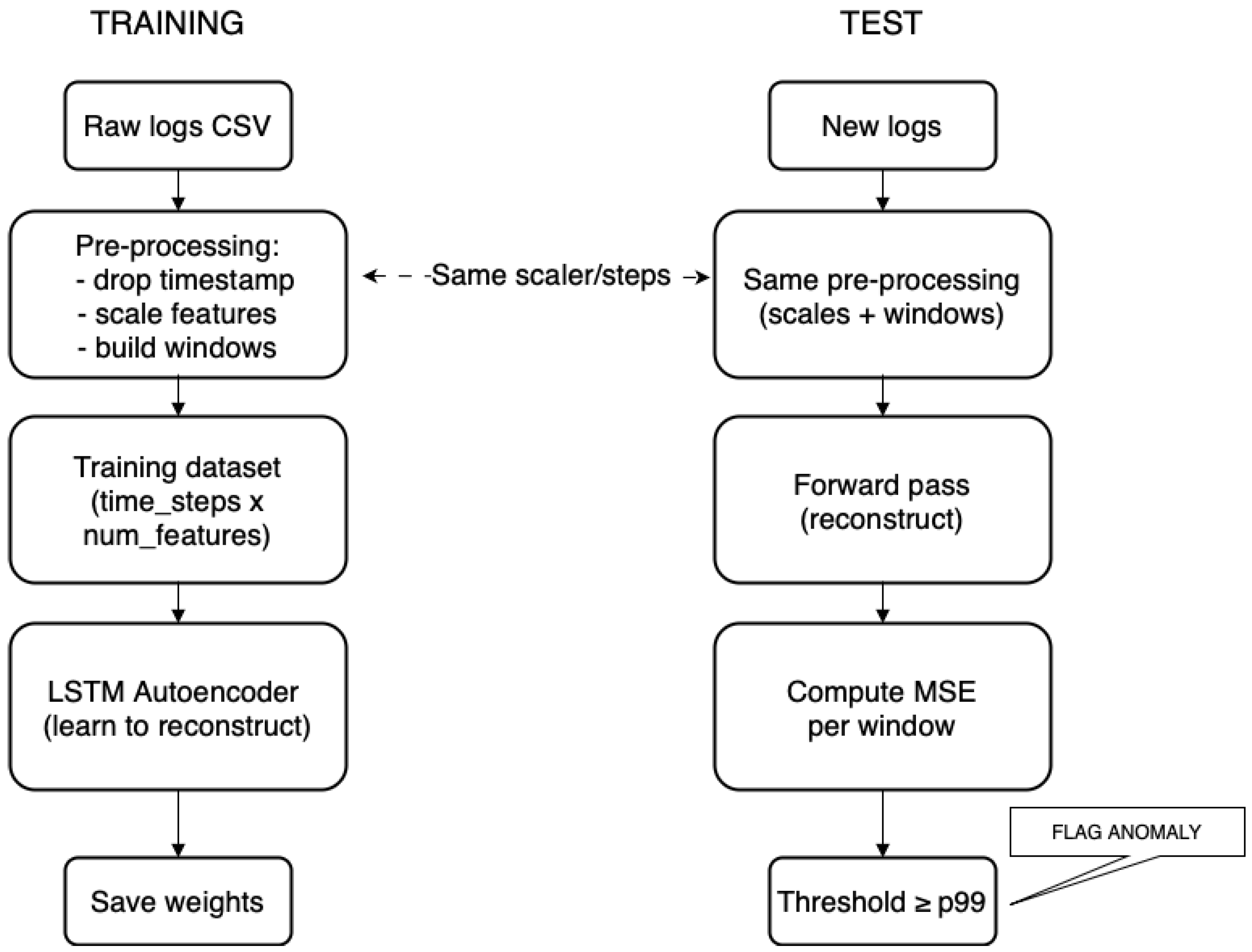
For anomaly detection, an LSTM autoencoder neural network was used Figure 2. The LSTM network is considered an extension of recurrent neural networks, but it is resistant to the phenomena of vanishing and exploding gradients [41]. As a recurrent network, it is applicable to all types of time series and has short-term memory, which transfers retained information from a certain past point in time to the current one. Additionally, it is enhanced with long-term memory, storing all previously retained information (differing from short-term memory, where one piece of information comes from a specific point) and making it available to the neuron in the current state. Internally, LSTM cells assess which information is important to remember in the context of the task being performed and update their internal state accordingly, and they can forget some information if it is deemed unnecessary after a certain time [42].

An autoencoder is a type of neural network trained without supervision. Its operation focuses on encoding unlabeled data. During the learning process, the autoencoder internally creates representations of the input data by discarding redundant and irrelevant information [42]. The autoencoder has a standard sequential structure, with input, hidden, and output layers, but the most characteristic division is the encoding, decoding, and bottleneck parts. The encoding part includes the initial layers from the input side, which are responsible for transforming the input data and placing them in the bottleneck, i.e., the hidden space of reduced dimensionality. In this configuration, data dimensionality reduction occurs, effectively compressing the data. In a typical autoencoder, this is achieved because the bottleneck layer contains fewer neurons than the others. The decoding part receives the encoded information from the bottleneck and performs the reverse transformation, which becomes the output of the entire network. The role of the autoencoder is to reproduce the input data as faithfully as possible at the output.

An LSTM autoencoder applies the autoencoder concept to a setup of LSTM neurons. In an LSTM autoencoder, both the encoding and decoding parts contain layers that are LSTM networks. LSTM autoencoders are successfully used to detect anomalies in various types of time series [42,43,44]. To find outliers, the data are subjected to the network, and then the reconstruction error is assessed, calculating how much the output data deviate from the input. A common measure of error in LSTM autoencoders is the mean squared error. It is necessary to establish a certain error threshold, beyond which the tested data are classified as anomalies. The underlying hypothesis is that if the network was infrequently trained using certain data or not at all, then accurately reconstructing these data would be difficult or impossible. Therefore, the larger the error, the more likely it is that the samples are anomalous. During network testing, detection was conducted on a large dataset (in a long sequence of measurements), and it was assumed that a certain percentage of anomalies existed within it, i.e., a percentile of the error distribution was rigidly chosen, with values to the left considered normal and those to the right as outliers.

The implementation of the LSTM autoencoder and anomaly detection was programmed in Python using TensorFlow, an open-source platform dedicated to ML, especially deep learning of neural networks. TensorFlow allows for the use of state-of-the-art ML methods, providing a rich set of tools and libraries commonly used in this field. It enables the execution of time-consuming calculations in parallel on multiple processors and graphics cores. While TensorFlow itself offers the option of distributed computing on multiple machines, according to the authors of the paper [45], this task is not the easiest and requires significant input from the programmer.

Horovod is a library that significantly simplifies the process of distributing calculations in TensorFlow. It supports the standard MPI for running parallel processes. Using it requires only minor modifications to the existing code. Internally, it operates by executing the ring-allreduce algorithm between training epochs, which is used here to average the gradients of the neural network distributed across multiple computing nodes. At the same time, ring-allreduce optimally utilizes the entire bandwidth of the computer network, while ensuring a sufficiently large buffer [45]. In short, in this algorithm, each of the n nodes communicates only with two neighbors. First, in $n-1$ iterations, a node adds received values to its local buffer, and in the next $n-1$ iterations, it replaces the values in its buffer with those received.

4.2.2. Design and Environment

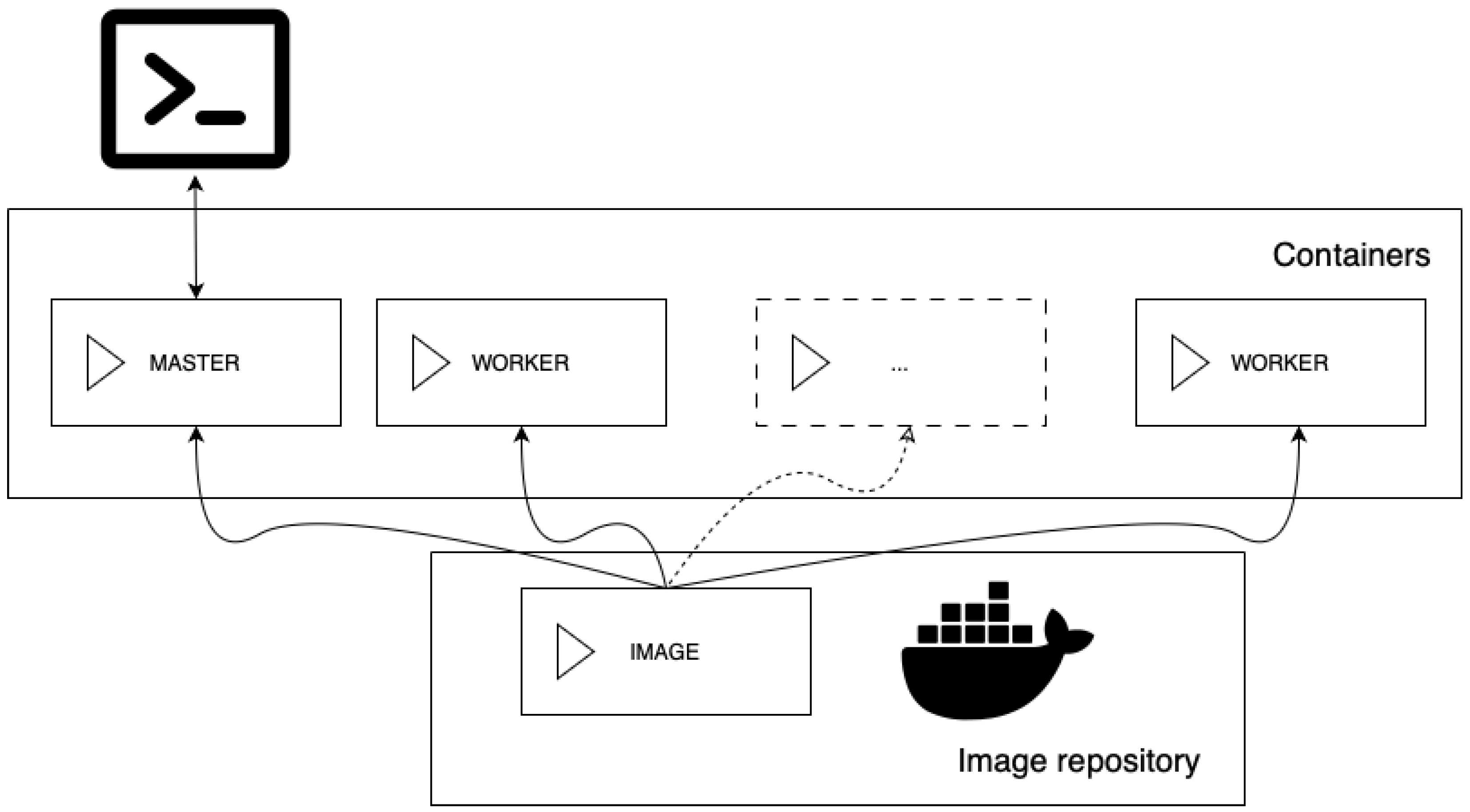
The application directory app, located in the same location as the compose.yml file of the virtual cluster, contains the folder src with Python scripts, the file requirements.txt with a list of required dependencies, and the folder data with training data. One of the files in this folder, used during this research, is named data.csv. It stores exactly 1820 samples taken from five containers, translating to 1805 training sequences with two attributes and a length of four time steps.

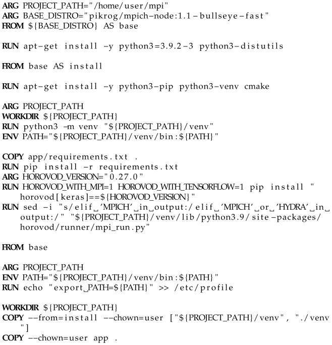
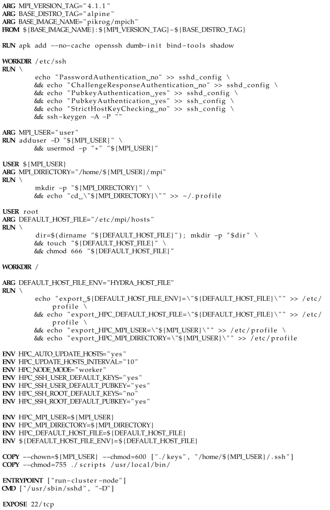
The script for building the container image with the anomaly detection application is presented in Listing 1. It employs a three-stage division, as used in the presented Dockerfiles. The resulting image extends a chosen cluster node image. In the first stage, the dependencies needed in the second stage and the final image are installed: the Python interpreter version 3.9.2, and tools for building and installing the Python modules (distutils) used by the TensorFlow library.

In the second stage, Python’s package manager pip, the virtual environment tool venv, and cmake, necessary for building the Horovod module, are installed. Using venv, a virtual environment is created in the standard project folder /home/user/mpi, and its location is added to the beginning of the PATH environment variable. This ensures that tools from this environment have priority over those in the global namespace when invoked. Then, the requirements.txt file containing the application’s dependency list is copied to the container. The package manager pip reads it and downloads the indicated packages. Horovod must be installed separately as it requires manual activation of MPI and TensorFlow support using environment variables prefixed with HOROVOD_WITH. Additionally, one of the source files of the Horovod module required a small correction (line 20). Horovod automatically determines the installed MPI implementation based on the text displayed by the command mpirun --version. In newer versions of MPICH, this command displays, among other things, the word HYDRA, the name of the new process manager, which Horovod does not yet recognize. The if condition responsible for detecting the MPI implementation was modified so that Horovod also accepts this current manager.

In the last stage, the PATH environment variable from the second stage is restored to reactivate the virtual environment. A command exporting this extended variable is added to the /etc/profile shell profile, ensuring it is always available, even after logging in via SSH.

Listing 1. Dockerfile for the anomaly detection.

Finally, from the second stage to the third, the prepared virtual environment is copied, and the remaining application files (scripts and training data) are transferred from the host system.

4.2.3. Implementation

This subsection only describes the most important parts of the source code of the anomaly detection application. In the project, training the neural network and detecting anomalies are divided into two separate scripts. For clarity, the code presented here is slightly modified and shortened, without additional helper functions, and all parameters stored in variables are hardcoded. In reality, most of these parameters can be changed from the command line.

Listing 2 shows a section of the code responsible for importing the necessary modules and setting parameters for ML and anomaly detection. The value normal_percentile=0.99 was chosen after a grid search (0.90–0.995) that maximized the F1-score on a hand-labeled validation subset; lower percentiles produced excessive false positives, whereas 0.995 missed short spikes.

Listing 2. Importing modules and functions. ML and anomaly detection parameters.

The variables in Listing 2 have the following purposes:

‑

csv_file—name of the file containing training data,

‑

time_steps—number of samples in a single training sequence,

‑

learning_rate—learning rate coefficient,

‑

optimizer—optimization algorithm used for calculating new weights during neural network training (Adam algorithm uses stochastic gradient descent),

‑

loss_function—loss function (MSE—Mean Squared Error),

‑

epochs—number of epochs (complete training cycles using the entire training set),

‑

callbacks—list of callbacks controlling the learning process,

‑

batch_size—size of the training batch (amount of data taken at once from the dataset during training),

‑

normal_percentile—the percentile of the error distribution, above which values will be classified as anomalies.

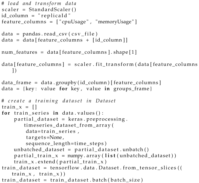
Before training, the data must be read from the source and appropriately transformed. The code segment in Listing 3 accomplishes this task. Data are read from a CSV file (line 6), then the unnecessary column storing the timestamp of the measurements is removed (line 7). The feature values are normalized using the StandardScaler object, which scales them by first subtracting their means and then dividing by their standard deviations (line 11). The table is then transformed into a dictionary mapping container instance IDs to their corresponding CPU and memory usage measurements (lines 13–14).

Next, each long sequence of measurements needs to be split into smaller subsequences of size time_steps, and then all subsequences are added to a master list. This is achieved using a helper function from the Keras module (line 19). In the given time series train_series, a window of size time_steps is moved from the beginning to the end, one step at a time, extracting the contained sequences. The mentioned function returns a Dataset object, but an array of numpy.array is needed, so the received object is transformed, and then appended to the master list train_x (lines 23–25).

The sequences stored in train_x serve as both input and output data for the neural network. The network aims to replicate the given time series of size time_steps as accurately as possible. Data from train_x are fed into the network, and output values close to the input are expected. A training set train_dataset is created based on train_x (line 26), and its batch size is determined using the batch method (line 27).

Listing 3. Code for reading and transforming training data.

The implementation of the LSTM autoencoder model is presented in Listing 4, and it was developed based on the article in [46]. The network consists of sequentially arranged layers. The first layer of the network is the input, with dimensions determined by the length of the time series fragment time_steps and the number of features num_features. By default, the input layer accepts a matrix with dimensions of four by two. The next two layers consist of LSTM cells and serve the purpose of encoding information. The first LSTM layer has one hundred and twenty-eight cells, and the second has sixty-four. In this arrangement, data reduction (compression) occurs. Additionally, each LSTM cell recursively develops as many times as the length of the time series time_steps (which is typically four steps). The first LSTM layer generates output signals for each individual sample taken from the time series (return_sequences set to True). As a result, for each of the one hundred and twenty-eight LSTM cells, four outputs are generated. In the second LSTM layer, cells have only one output each, and the signal is only generated after processing the last (fourth) sample from a given sequence.

A RepeatVector layer, serving as a kind of ‘bridge’, separates the encoding and decoding parts. It replicates the signals received from the output of the encoding part (from the second LSTM layer) as many times as the length of the time series time_steps. This step is necessary because the second LSTM layer merges the input matrix and removes the dimensions determined by time_steps, meaning that it returns a vector of encoded information at the output. The third and fourth LSTM layers decode information and have sixty-four and one hundred and twenty-eight cells, respectively, each developing four times (which resembles the encoding part, but arranged in the opposite direction). Both generate output signals for each processed sample (return_sequences is true). The final layer is a densely connected neural network (Dense), with a number of neurons equal to the number of features specified by num_features. There is also an intermediate TimeDistributed layer before Dense. At each timestep, the fourth LSTM layer produces one hundred and twenty-eight output signals simultaneously. Simply put, TimeDistributed combines these signals into single outputs, consequently leading to four outputs for each Dense neuron. In this way, the autoencoder ultimately returns a matrix at its output with the same dimensions as the input matrix.

Before training and using the neural network, its model must be compiled using the compile method (line 13). In the arguments of this function, the optimization algorithm and the loss function are set. The fit method (line 16) initiates the neural network training process. This requires the training set to be passed. Additionally, the number of epochs (epochs) and the list of callbacks (callbacks), which is normally empty, are specified. Callbacks allow for intervention in the training process and are triggered at various stages. They can be used, for example, to prematurely terminate training (if subsequent epochs do not improve the quality of the neural network) or to create checkpoints (especially useful for networks requiring time-consuming training). The fit function returns a History object that contains information about the training process. Among other things, it allows one to read how the metrics evaluating how well the neural network is replicating input values have changed over the epochs.

Listing 4. Neural network model code for anomaly detection. Based on [46].

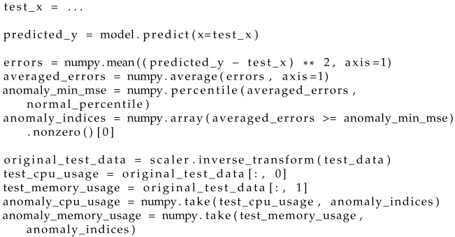
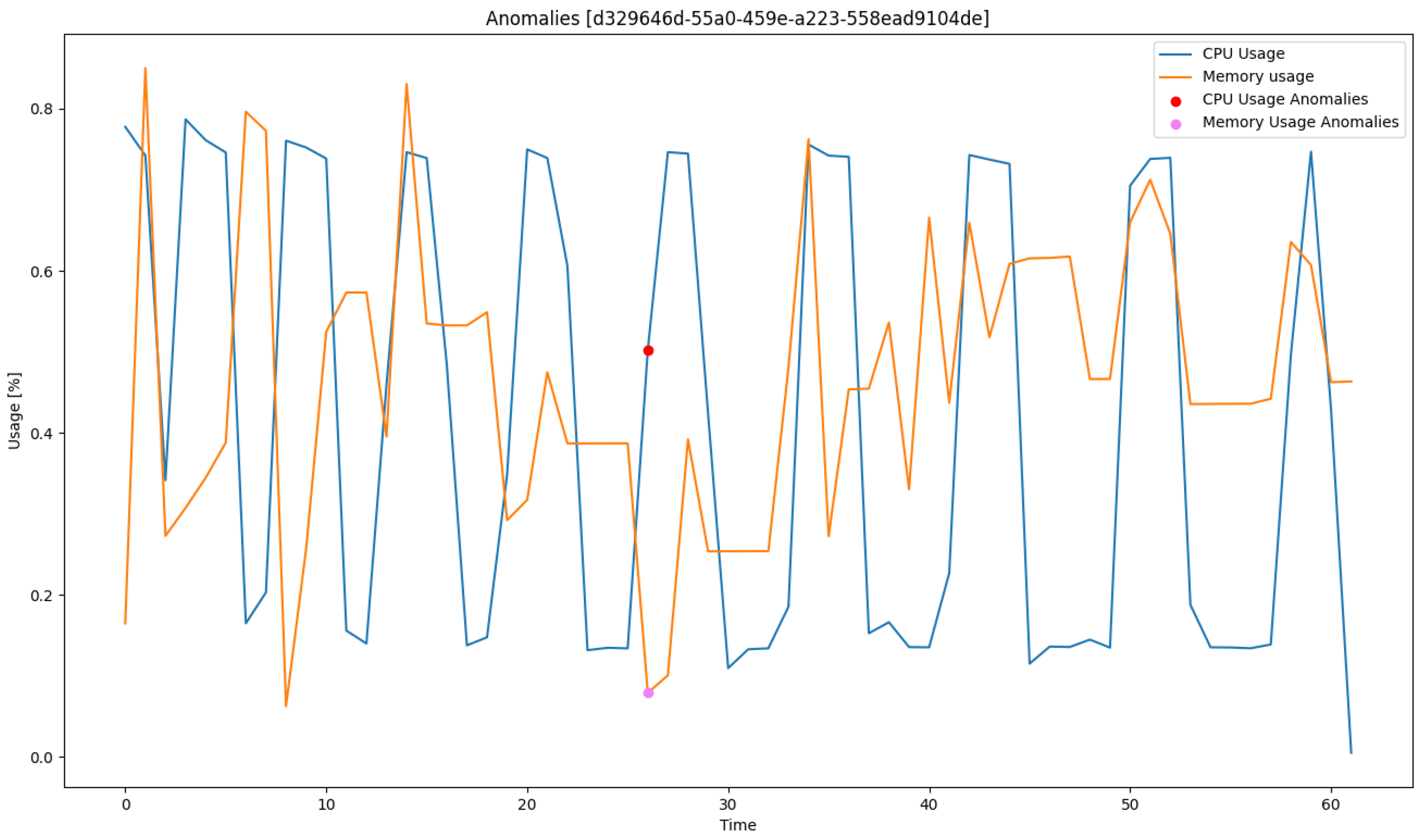
After training the network, it can be used for anomaly detection. The code responsible for this is included in Listing 5. It is assumed that the test data stored in test_x have the same structure as the training data in train_x and have been previously normalized. The test data are fed into the autoencoder (line 3). Based on the network’s response, mean squared errors are calculated between the received and actual time series (line 5). The resulting errors are determined separately for CPU load and memory usage measurements. Then, these errors are averaged in pairs for individual samples (line 6), resulting in a one-dimensional vector. In the distribution of errors, a percentile that separates normal values from outliers is found (line 7), based on which indices of time segments classified as anomalies are identified in the test data (line 8). Knowing these indices, outlier samples can be extracted from the original (i.e., unnormalized) test data (lines 10–14), and then visualized on a time plot, as exemplified in Figure 3. The colored dots symbolize the occurrence of anomalies in the time plots.

Listing 5. Code for anomaly detection with a trained network.

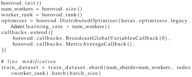
Up to this point, the implementation has only been discussed using the TensorFlow library. To enable distributed learning across multiple machines, one should add (preferably at the top of the script) the Horovod configuration code, which is presented in Listing 6. The Horovod environment is initialized (line 1), the number of parallel processes is obtained (line 2), and the rank of the current process is determined (line 3). The chosen optimization algorithm should be wrapped in a DistributedOptimizer object (line 4), which implements an algorithm for calculating gradients at the level of a single process and updating weights only after collecting gradients from all parallel processes [45]. In the documentation, Horovod recommends accelerating learning (in terms of the weight value increase, not time reduction) by multiplying the learning rate by the number of processes. Procedures were added to the callback list for propagating global variables from the master process to the others (line 6) and for averaging the neural network metrics (line 7).

Listing 6. Horovod initialization and configuration. Based on [45] and documentation.

The Horovod platform is now ready for operation. What remains is the division of the training set among the workers, as this will enable a gain in efficiency. In the code from Listing 3, line 27 was modified to the fragment from Listing 6 at line 11. The shard method divides the dataset into as many parts as there are processes (num_workers) and selects one of them based on the rank of the process (worker_rank).

4.2.4. Methodology Supplement

Research with this application was only conducted for the scenario in which a parallel application operates in Docker containers, with its processes distributed among many containers in such a way that each container runs a maximum of one process. Such a distribution strategy forces the MPI implementation to engage the network stack for inter-process communication. There is a need to pass two environmental variables to the script. When running a program through docker exec in a container shell, it is possible to define custom environmental variables for it using the -e argument, as in Listing 7. The PYTHONHASHSEED variable sets the seed for the hash() hash generator. Assigning it a specific constant is one of the necessary steps to ensure reproducibility of neural network training. The TF_CPP_MIN_LOG_LEVEL variable allows filtering the messages printed by the TensorFlow module on the console screen. Assigning a value of two to it means silencing regular information and warnings, while errors will still be displayed.

Listing 7. Executing a command in the master node’s shell with exported environmental variables.

To ensure that the given environmental variables are properly propagated to all parallel processes run by mpirun, it is necessary to use the appropriate option in the command line. In MPICH, this is achieved with the -genvlist argument, after which a list of variable names separated by commas is provided (Listing 8), and in OpenMPI, it is the -x argument, after which a single variable can be listed (Listing 9).

To run a single test, the command from Listing 10 is used. The script conducts neural network training on data from the data.csv file. The provided options have the following meanings:

‑

--distributed—distributed mode (initiates the Horovod environment and enables MPI support),

‑

--epochs 100—one hundred training epochs,

‑

--batch 64—a batch size of sixty-four sequences,

‑

--seed 1234—fixed setting of pseudorandom number generators’ seed (to ensure reproducibility of the resulting neural network),

‑

--no-early-stopping—no early termination of training before the set number of epochs,

‑

--no-output-model—the model will not be saved to a file (not needed for research),

‑

--silent—turning off the display of information about the progress of training.

Listing 8. Running a test for the “MPICH Network” scenario. Propagation of environmental variables.

Listing 9. Running a test for the “OpenMPI Network” scenario. Propagation of environmental variables.

Listing 10. Executing a single test with the anomaly detection application.

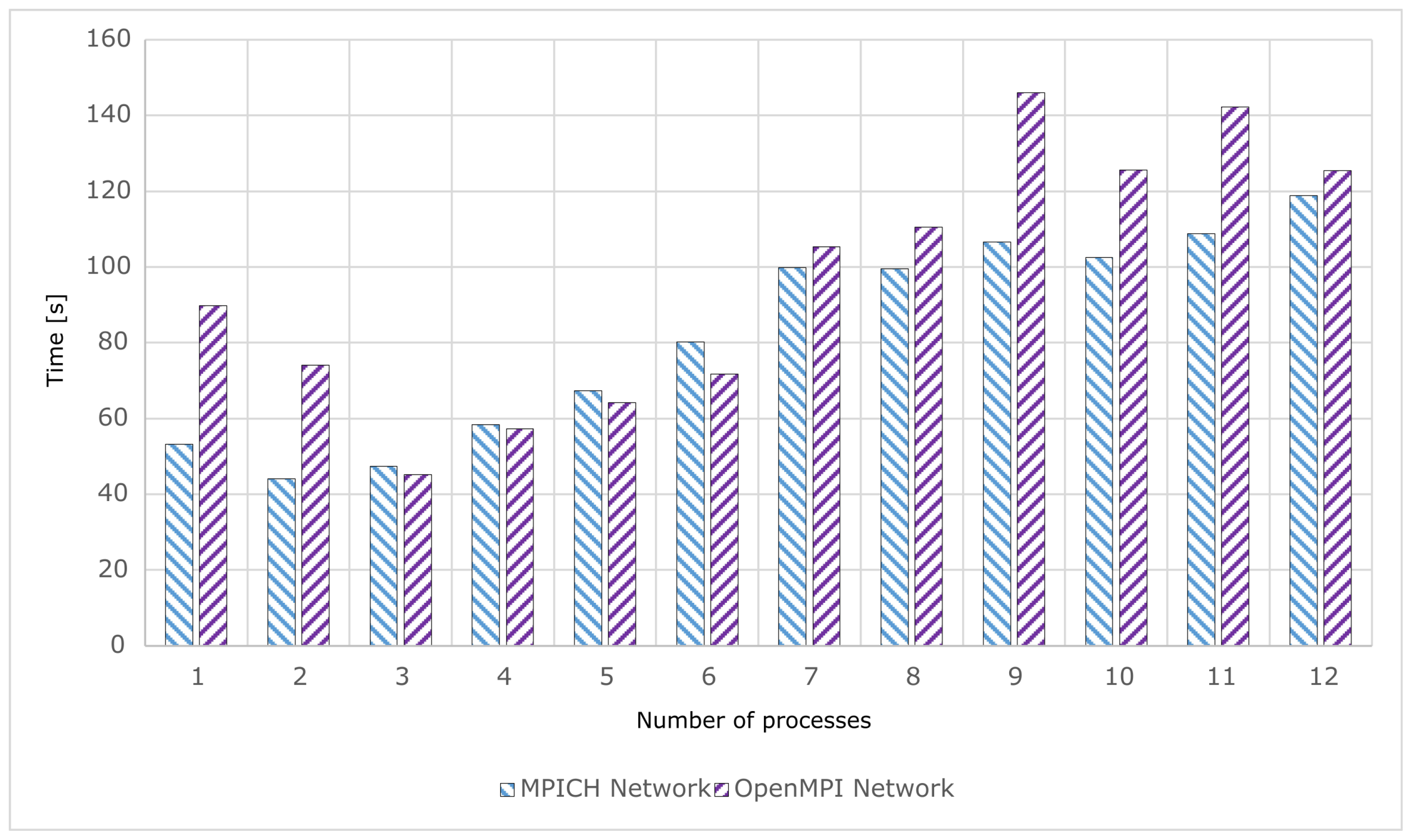
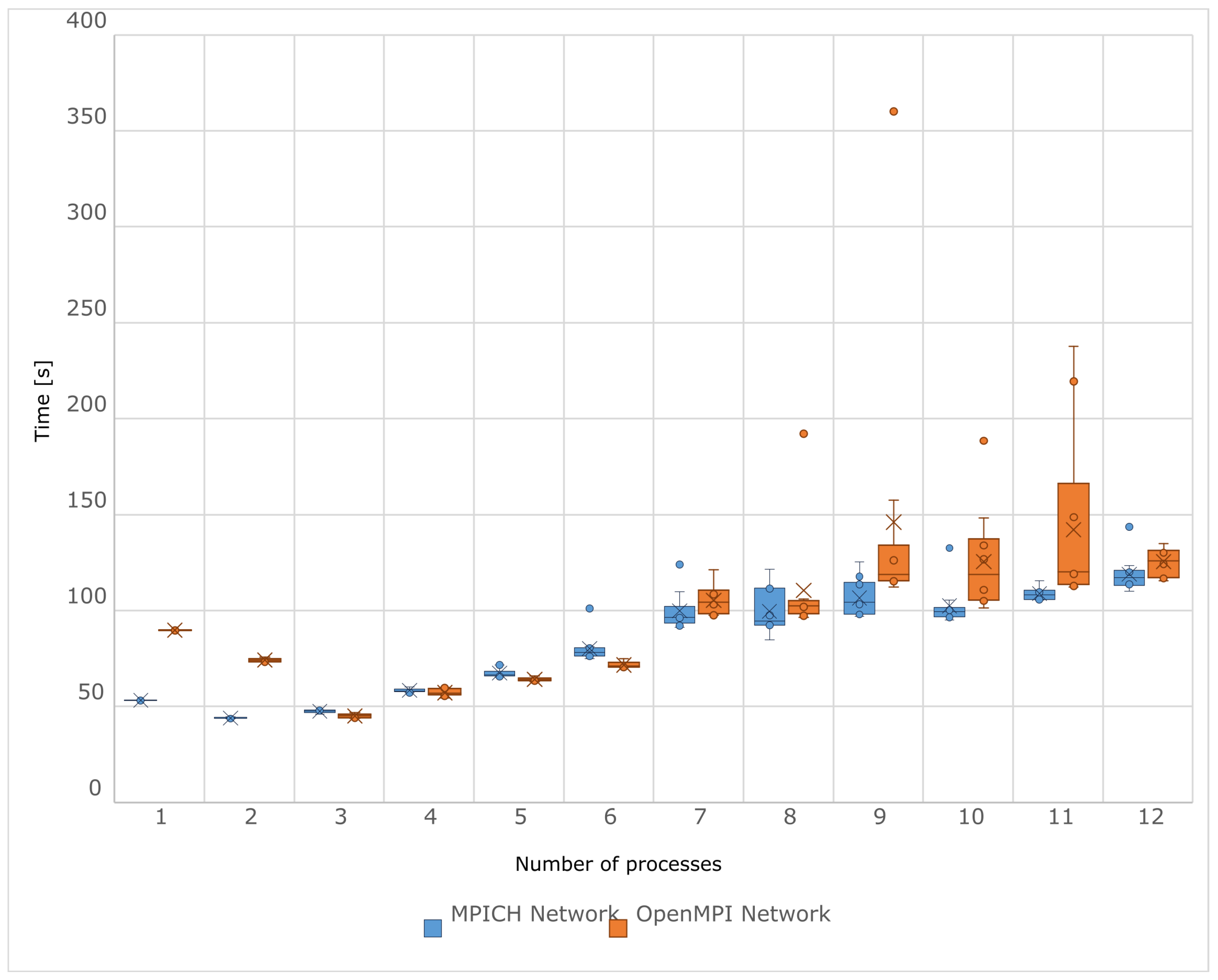
The chart in Figure 4 shows the average execution times of the ML application for the MPICH and OpenMPI implementations. The time gain achieved due to distributed computing was not as satisfying as with applications for prime number searching and integration. With the MPICH implementation, neural network training averaged the shortest duration, with two processes, and with OpenMPI, with three processes (

Table 2. Average execution times of a neural network training application. One process per container. Performance comparison of MPICH and OpenMPI implementations.

${\mathit{n}}_{\mathit{p}}$	${\mathit{t}}_{\mathbf{avg}}$ [s]		An Absolute Improvement [s]	Relative Improvement [%]
	OpenMPI	MPICH
1	89.761	53.270	36.491	40.654
2	74.169	44.024	30.145	40.643
3	45.129	47.449	2.320	4.889
4	57.258	58.395	1.137	1.948
5	64.139	67.359	3.221	4.781
6	71.675	80.180	8.505	10.607
7	105.357	99.827	5.529	5.248
8	110.490	99.555	10.936	9.897
9	146.067	106.561	39.506	27.046
10	125.540	102.463	23.077	18.382
11	142.171	108.794	33.377	23.477
12	125.471	118.918	6.553	5.223

). For larger numbers of processes, the average test times noticeably increased. MPICH performed worse in this regard, as the tests started to take longer from four processes upwards, compared to running exactly one process of the tested application. The same can be said for OpenMPI, but from seven processes upwards. In terms of performance, MPICH performed better than OpenMPI, especially with one and two processes. According to

Table A1. Measuring the training time of a neural network. One process per container. MPICH implementation.

${\mathit{n}}_{\mathit{p}}$	${\mathit{n}}_{\mathit{r}}$	${\mathit{t}}_{\mathit{min}}$ [s]	${\mathit{t}}_{{\mathit{q}}_1}$ [s]	${\mathit{t}}_{\mathit{med}}$ [s]	${\mathit{t}}_{\mathit{avg}}$ [s]	${\mathit{t}}_{{\mathit{q}}_3}$ [s]	${\mathit{t}}_{\mathit{max}}$ [s]	${\mathit{t}}_{\mathit{std}}$ [s]
1	9	53.021	53.156	53.268	53.270	53.383	53.488	0.148
2	10	43.577	43.802	43.903	44.024	44.343	44.552	0.343
3	10	46.064	47.015	47.618	47.449	48.112	48.256	0.799
4	10	57.275	57.725	57.951	58.395	58.842	60.255	1.099
5	10	65.240	66.171	66.559	67.359	67.122	71.644	2.312
6	10	74.993	76.318	78.303	80.180	80.020	101.006	7.585
7	10	91.379	94.081	96.577	99.827	99.500	123.990	9.992
8	10	84.615	92.779	94.580	99.555	108.013	121.440	11.592
9	10	96.947	98.774	104.238	106.561	111.820	125.296	9.472
10	10	94.960	97.464	99.466	102.463	100.205	132.552	10.936
11	10	105.364	106.090	108.167	108.794	110.123	115.514	3.232
12	10	109.960	114.075	117.133	118.918	119.348	143.533	9.492

, training with MPICH was almost 41% faster in those cases. For numbers of processes from three to eight, the average test times for both implementations were practically the same. Then, in the range from nine to eleven processes, significant deviations occurred, to the detriment of OpenMPI by about 23–40%.

However, the values obtained are quite unreliable for numbers of processes greater than four. The chart in Figure 5 provides a better view of the analyzed measurements. With MPICH, when the number of processes did not exceed four, the distribution of measurements showed no significantly deviating values, its range was narrow, and the average values were very close to their corresponding medians. Unfortunately, for larger numbers of processes, the opposite situation was observed. The same occurred with the OpenMPI implementation, but questionable measurements only started from seven processes upwards. Particularly concerning are the outliers, such as the one obtained at nine processes with the OpenMPI implementation: one of the tests lasted almost 360 s, but the median of the measurements was about 118 s, and the minimum value was about 112 s. Overall, the OpenMPI implementation seemed more prone to measurement fluctuations with large numbers of processes. Therefore, measurements from a certain number of processes ceased to be stable and fundamentally lost quality. In this situation, instead of the average, it may be more reasonable to analyze the median, which is a measure characterized by resistance to extreme values. However, it is advisable to take the obtained results with a large dose of skepticism. Less reliable sets of measurements can be quickly recognized by a significantly elevated standard deviation.

However, the question remains as to why, at least in the current configuration, it is so difficult to obtain meaningful measurements. Special attention should be paid to the specifics of the computational process. The application creates many computational threads, the number of which is optimized depending on the available processor cores. The developers of TensorFlow wisely did not consider the case where someone would try to disperse computations on a single, local machine in a roundabout way, namely by creating multiple processes of such an application, instead of relying on built-in procedures that automatically manage parallel computations. Proceeding in this way quickly leads to the saturation of the operating system’s capacity for task management. Too many threads and processes cause excessive context switching. Additionally, the size of a neural network means that many operations are performed in an extensive memory space. Consequently, with a large number of processes, cache thrashing (a phenomenon well known for its performance costs) likely occurs too frequently.

Table 3. Average execution times of the neural network training application. One process per container. MPICH implementation. Comparison of measured, expected, and ideal times.

${\mathit{n}}_{\mathit{p}}$	${\mathit{t}}_{\mathit{avg}}$ [s]	${\mathit{t}}_{\mathit{pred}}$ [s]	${\mathit{t}}_{\mathit{id}}$ [s]	$\frac{|{\mathit{t}}_{\mathit{avg}}-{\mathit{t}}_{\mathit{pred}}|}{{\mathit{t}}_{\mathit{avg}}}·100$ [%]	$\frac{|{\mathit{t}}_{\mathit{avg}}-{\mathit{t}}_{\mathit{id}}|}{{\mathit{t}}_{\mathit{avg}}}·100$ [%]
2	44.024	26.635	26.635	39.500	39.500
3	47.449	29.349	17.757	38.145	62.577
4	58.395	35.587	13.317	39.059	77.194
5	67.359	46.716	10.654	30.646	84.183
6	80.180	56.133	8.878	29.992	88.927
7	99.827	68.726	7.610	31.155	92.377
8	99.555	87.349	6.659	12.260	93.312
9	106.561	88.493	5.919	16.956	94.446
10	102.463	95.905	5.327	6.400	94.801
11	108.794	93.148	4.843	14.381	95.549
12	118.918	99.728	4.439	16.137	96.267

was used to analyze the scalability of the prepared application operating with the MPICH implementation. The graph and table confirm the earlier observations regarding the modest time gain from distributed computing. The expected characteristic diverged significantly from the points plotted for the measured times (in the worst case by almost 40% at two processes), not to mention the distance from the ideal characteristic, where the relative difference accumulated to about 96%. The increasing segments of the expected characteristic also signal weak scalability. With the OpenMPI implementation, for which an analogous

Table 4. Average execution times of a neural network training application. One process per container. OpenMPI implementation. Comparison of measured, expected, and ideal times.

${\mathit{n}}_{\mathit{p}}$	${\mathit{t}}_{\mathit{avg}}$ [s]	${\mathit{t}}_{\mathit{pred}}$ [s]	${\mathit{t}}_{\mathit{id}}$ [s]	$\frac{|{\mathit{t}}_{\mathit{avg}}-{\mathit{t}}_{\mathit{pred}}|}{{\mathit{t}}_{\mathit{avg}}}·100$ [%]	$\frac{|{\mathit{t}}_{\mathit{avg}}-{\mathit{t}}_{\mathit{id}}|}{{\mathit{t}}_{\mathit{avg}}}·100$ [%]
2	74.169	44.880	44.880	39.489	39.489
3	45.129	49.446	29.920	9.565	33.701
4	57.258	33.847	22.440	40.887	60.809
5	64.139	45.806	17.952	28.583	72.010
6	71.675	53.449	14.960	25.429	79.128
7	105.357	61.436	12.823	41.688	87.829
8	110.490	92.187	11.220	16.566	89.845
9	146.067	98.214	9.973	32.761	93.172
10	125.540	131.460	8.976	4.716	92.850
11	142.171	114.128	8.160	19.725	94.260
12	125.471	130.323	7.480	3.867	94.038

is provided, the scalability of the application seemed less predictable, as determined by the irregular outline of the expected characteristic. Here, the greatest deviation in the time characteristic from the obtained average values reached about 41%, and for the ideal characteristic, the difference accumulated to 94%; so in this respect, OpenMPI performed similarly to MPICH.

The participation of inter-process communication in the context of the overall program is significant in the case of the currently analyzed application. This mainly results from the fact that between each training epoch, there is synchronization of processes and averaging of weights in distributed neural networks using the allreduce method. It should be remembered that the time cost of the allreduce algorithm performed between training epochs increases with the addition of more processes, because the neural network is not divided among sub-processes. Each of them has an identically sized structure. Therefore, the more processes, the more time needs to be allocated for averaging weights.

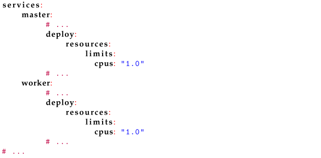
Since the mediocre scalability resulted partly from the overload of resources such as the processor, it might be possible to improve this by imposing restrictions on its use. Docker allows setting limits on the usage of processor time for containers. Listing 11 shows how to enable this function for a virtual cluster. Conventionally, the value of the cpus option denotes the maximum number of cores allocated to the container. In practice, the level of restriction affects the time allocation of the container’s tasks to the processor. For example, if there are two cores in the computer and the modification from Listing 11 is applied, the container will be able to load the processor to a maximum of 50% of its capacity per second.

Listing 11. Limiting processor time for cluster containers.

After applying the changes from Listing 11, tests were repeated for both implementations. Thanks to the limitation on processor time with MPICH, the scalability was artificially slightly improved, as can be inferred from

Table 5. Average execution times of a neural network training application. One process per container. MPICH implementation. CPU time limit. Comparison of measured, expected, and ideal times.

${\mathit{n}}_{\mathit{p}}$	${\mathit{t}}_{\mathit{avg}}$ [s]	${\mathit{t}}_{\mathit{pred}}$ [s]	${\mathit{t}}_{\mathit{id}}$ [s]	$\frac{|{\mathit{t}}_{\mathit{avg}}-{\mathit{t}}_{\mathit{pred}}|}{{\mathit{t}}_{\mathit{avg}}}·100$ [%]	$\frac{|{\mathit{t}}_{\mathit{avg}}-{\mathit{t}}_{\mathit{id}}|}{{\mathit{t}}_{\mathit{avg}}}·100$ [%]
2	140.129	100.240	100.240	28.466	28.466
3	121.436	93.419	66.827	23.072	44.970
4	119.361	91.077	50.120	23.696	58.010
5	109.369	95.489	40.096	12.691	63.339
6	117.447	91.141	33.413	22.398	71.550
7	133.815	100.669	28.640	24.770	78.597
8	124.552	117.088	25.060	5.993	79.880
9	131.276	110.713	22.276	15.664	83.032
10	136.289	118.149	20.048	13.310	85.290
11	128.117	123.899	18.225	3.292	85.774
12	127.043	117.440	16.707	7.559	86.850

. However, the results obtained were still not satisfactory. The minimum execution time shifted to five processes, and the expected characteristic became slightly more uniform. The greatest relative deviation in the expected characteristic from the average time dropped to about 28%. Unfortunately, the same could not be demonstrated with the OpenMPI implementation, as the time for each subsequent process always increased for unexplained reasons.

It has been shown that more advanced and practical applications (not necessarily written in C++) can be run on a virtual cluster. To some extent, it has been proven that a cluster is suitable for demonstrating the acceleration of calculations through algorithm parallelization. However, a certain weakness of containerization became apparent. Difficulties in confirming the scalability of distributed ML in Tensorflow partly stem from the use of virtualization at the operating system level. The limitation on the allocated processor time is not sufficient as isolation. If it were possible to attach virtual cores to containers, Tensorflow, having access to only a small set of cores, would create fewer threads per process.

5. Conclusions

This research conducted on Docker-container-based clusters within HPC environments has yielded several significant insights, successfully achieving the construction and launch of a Docker-container-based cluster. This feat was complemented by the creation of a clear, detailed instructional manual for replicating such clusters. The methodology applied in the research was meticulously detailed, including the characterization of the computing platform used for measurements, thus providing a comprehensive guide for future endeavors in similar settings.

A key aspect of this research was the demonstration and performance testing of parallel applications. A more advanced Python application utilizing ML for anomaly detection in system logs was successfully implemented and run on the virtual cluster. This application trained a neural network to examine sample logs for suspicious deviations, showcasing the practical application of advanced technologies in a containerized environment. The study also included a critical evaluation of the performance overhead associated with containerization. An interesting finding of the research was the partial loss of computational power caused by Docker. The performance overhead of containerization was found to depend on various factors, including the application itself, the MPI implementation, and the security mechanisms operating within the container. Docker’s ability to disable many security features, thereby minimizing the performance drop to an acceptable level, was also noted, though this involved certain risks.

The comparisons made throughout the work between the MPICH and OpenMPI implementations provided a broader perspective on how containerization affects the performance of a virtual cluster. In tests with example programs, MPICH often outperformed OpenMPI in terms of execution time, but this was not a universal rule, as test results could significantly differ with other applications and environments. The study emphasized that performance is not the only criterion for deciding on an MPI implementation; other aspects such as technical support, tools and extensions for programming parallel applications, process configuration and management, and compliance with the MPI standard are also considered important.

The research suggested that a containerized cluster could find application in real, high-performance solutions requiring large amounts of computational power. It opened the possibility of running a virtual cluster on a physical HPC cluster for quick and trouble-free deployment of parallel applications. However, it is also acknowledged that this research did not conclusively determine whether containerization would cause significant performance losses in this scenario. This leaves an open avenue for future research, particularly in exploring the overhead involved in running an application on a real HPC cluster, compared to containers connected by a Swarm network. These studies should be repeated, but on a cluster operated in a Swarm distributed mode, where each container would be located on a different computer (these computers could be virtual machines, although it would be preferable to use physical ones). Presumably, such an arrangement would work in favor of the application’s scalability and, above all, it should result in better quality time measurements. Table A1 and 

Table A2. Measuring the training time of a neural network. One process per container. OpenMPI implementation.

${\mathit{n}}_{\mathit{p}}$	${\mathit{n}}_{\mathit{r}}$	${\mathit{t}}_{\mathit{min}}$ [s]	${\mathit{t}}_{{\mathit{q}}_1}$ [s]	${\mathit{t}}_{\mathit{med}}$ [s]	${\mathit{t}}_{\mathit{avg}}$ [s]	${\mathit{t}}_{{\mathit{q}}_3}$ [s]	${\mathit{t}}_{\mathit{max}}$ [s]	${\mathit{t}}_{\mathit{std}}$ [s]
1	9	89.541	89.712	89.770	89.761	89.840	89.900	0.109
2	10	73.149	73.469	73.999	74.169	74.820	75.611	0.847
3	10	43.819	44.235	45.070	45.129	45.799	46.715	1.046
4	10	54.420	56.157	56.958	57.258	58.852	59.946	1.833
5	10	62.790	63.488	63.892	64.139	64.785	65.812	0.919
6	10	70.168	70.624	71.014	71.675	72.489	74.969	1.597
7	10	97.455	98.687	104.448	105.357	109.869	121.326	7.752
8	10	96.536	99.271	102.474	110.490	104.620	192.168	28.874
9	10	112.303	116.078	118.782	146.067	124.329	360.184	76.341
10	10	101.444	105.889	118.811	125.540	132.559	188.460	26.920
11	10	112.160	114.202	120.140	142.171	141.852	237.766	46.954
12	10	115.555	118.950	125.956	125.471	130.566	134.903	7.014

contain details summarizing the measurements made in this part of the research.

Future efforts will explore classification model behavior for container structure and reinforcement-learning-driven auto-scaling policies.