Machine Learning Approach for Ground-Level Estimation of Electromagnetic Radiation in the Near Field of 5G Base Stations

Featured Application

Electromagnetic radiation is a highly relevant and compelling application, particularly given the rapid expansion of 5G networks and the rising public concern about their potential health and environmental effects. Utilizing a machine learning-based approach to estimate ground-level electromagnetic radiation (EMR) near 5G base stations provides a powerful solution that combines accuracy with scalability. Consequently, this approach provides a guide for the adoption and deployment of 5G technology in Africa, with a specific interest in Nigeria.

Abstract

Electromagnetic radiation measurement and management emerge as crucial factors in the economical deployment of fifth-generation (5G) infrastructure, as the new 5G network emerges as a network of services. By installing many base stations in strategic locations that operate in the millimeter-wave range, 5G services are able to meet serious demands for bandwidth. To evaluate the ground-plane radiation level of electromagnetics close to 5G base stations, we propose a unique machine-learning-based approach. Because a machine learning algorithm is trained by utilizing data obtained from numerous 5G base stations, it exhibits the capability to estimate the strength of the electric field effectively at every point of arbitrary radiation, while the base station generates a network and serves various numbers of 5G terminals running in different modes of service. The model requires different numbers of inputs, including the antenna’s transmit power, antenna gain, terminal service modes, number of 5G terminals, distance between the 5G terminals and 5G base station, and environmental complexity. Based on experimental data, the estimation method is both feasible and effective; the machine learning model’s mean absolute percentage error is about 5.89%. The degree of correctness shows how dependable the developed technique is. In addition, the developed approach is less expensive when compared to measurements taken on-site. The results of the estimates can be used to save test costs and offer useful guidelines for choosing the best location, which will make 5G base station electromagnetic radiation management or radio wave coverage optimization easier.

1. Introduction

The current advancement in telecommunication standards is represented by the fifth generation (5G) of mobile networks, which offer far more than the 4G/LTE networks. The demands of mobile network users, as well as those imposed by cutting-edge ideas like connected and autonomous cars, smart factories, or smart cities, are satisfied by 5G technology [1,2,3,4]. In contrast to 4G/LTE networks, 5G has substantially greater data throughput (peak rate up to 20 Gbps), much lower latency (no more than 1 ms), much higher dependability (99.999%), and the capacity to serve a much higher number of terminals (device density up to one million per square kilometer) [3,5,6,7,8,9,10,11,12,13,14,15,16]. On the other hand, electromagnetic waves are significantly impacted by the environment, despite the widespread deployment of 5G base stations. Therefore, in order to guarantee compliance with regulatory restrictions and to provide the best site selection for radio wave coverage, it is important to assess the electromagnetic radiation intensity of 5G base stations. Electromagnetic waves have a wide range of practical applications in daily life, including communication via cell phones, radio broadcasting, WiFi, cooking, vision, medical imaging, and cancer treatment (see Figure 1). There are now four primary methods to determine the electromagnetic radiation intensity of base stations: time-series analysis [17,18], electromagnetic modeling [11,12,13,14], measurement near base stations using a field-strength analyzer [4,5,6,7,8,9,10], and extrapolation methodology [15,16,17]. Other classes of methods include the following: indirect measurement methods, environmental measurement methods, wireless and remote sensing methods, biological and health impact measurements, mathematical and statistical approaches, and regulatory and compliance testing.

While measurement is the standard technique for accurately estimating the quantity of electromagnetic radiation near 5G base stations, it has the drawback of being very time-consuming and expensive to monitor. In comparison to the method of moments (MOMs) and the finite difference time domain (FDTD), ray tracing and its acceleration algorithm offer a new approach for complicated electromagnetic environment prediction in a broad area with improved processing efficiency. The ray tracing algorithm’s basic idea is to solve every path between base stations and field points and then use path information to calculate the electric field strength at each field point. The simulation software based on the ray tracing technique can quickly and reliably forecast the electromagnetic field (EMF) at various sites near base stations after importing transmitted antennas, nearby structures, and terrain features. However, because of three-dimensional beamforming, massive multiple-input and multiple-output (MIMO), and other novel features of 5G base stations [18,19,20,21,22], the electromagnetic radiation intensity is greatly impacted by the locations, service modes, and quantity of 5G terminals in real-world scenarios. These factors are challenging to simulate in the simulation software. The following is an overview of the main features and benefits of massive MIMO and beamforming in 5G base stations:

• Better Coverage and Signal Quality: Massive MIMO extends coverage regions and enhances signal quality, even in highly congested urban locations, by utilizing beamforming and spatial multiplexing. This gives rise to improved user connectivity. Beamforming directs the transmitted energy toward the terminals instead of scattering it in different directions, as seen in Figure 2. In addition, by tracking the signals emanating from the terminals, the base station dynamically tracks their movement and modifies the ideal transmission direction.
• Better User Capacity: The base station serves more users simultaneously and mitigates congestion using a large number of elements (up to 256).
• Reduction of Interference: By spatially separating signals, interference is mitigated, consequently improving the signal-to-noise ratio and overall network performance.
• Energy Efficiency: By concentrating transmission power where it is required instead of dispersing evenly in all directions, massive MIMO is energy-efficient despite its higher antenna requirement.

The extrapolation technique uses measurements made over a short period to determine the maximum level of the electromagnetic field generated by a base station [15]. The scheduler must, however, continually allot all available resources to one user for at least six minutes, leaving all other users in standby mode, in order to accurately estimate the maximum level. This leads to an unfeasible loss of data connection of at least six minutes. In order to overcome this restriction, the extrapolation method approximates the maximum radiation field intensity by using the synchronization signal block (SB) in conjunction with specific extrapolation factors. Even with this improvement, the method still requires laborious computation processes and has high testing costs.

Predicting the time-varying electromagnetic radiation in the vicinity of base stations is another common use for time-series analysis. For instance, Zeydin Pala et al. constructed a data set based on 36-month recorded EMF and forecasted the upcoming 12-month EMF using traditional models and artificial neural network (ANN) models, respectively [18]. Pietro De Lellis et al. developed a time-series analysis model based on data collected over a period of seven days in order to forecast the electric field on weekdays and weekends, as well as the peak exposure time of the day [19]. These models are able to accurately predict the future trend of radiation levels close to base stations based on historical data.

In situ RF exposure measurement surveys have been conducted for several 5G commercial networks globally [2,3,4,5,6,7]. These surveys not only measure the actual exposure levels, which include the power density (or field strength) from the base station (BS) under current operating conditions (such as traffic load, number of connected devices, their distribution, and scheduled beams), but also assess the potential maximum exposure levels. For a specific measurement location or point of interest (POI), the maximum exposure corresponds to the power density when the BS is transmitting at full power, which represents a scenario where the BS operates at 100% capacity. To estimate this, appropriate extrapolation techniques for 5G BSs have been discussed in the literature [7,9,10,11,12] and incorporated into relevant standards [13]. These methodologies are applicable to both frequencies below 6 GHz and higher frequency bands [14]. However, as emphasized in [15], 5G networks operating at millimeter-wave (mmW) frequencies pose unique challenges that must be taken into account when conducting EMF exposure measurements. The examples are as follows:

• For the use of directional antennas or, alternatively, single-axis omnidirectional probes when conducting EMF assessments with directional antennas, careful positioning is essential to capture exposure contributions from all relevant directions.
• The shorter wavelength enables the use of a greater number of antenna elements. As a result, the antenna beamwidth may be narrower compared to that of typical massive MIMO (m-MIMO) base stations operating below 6 GHz.

However, machine learning regression algorithms are crucial for forecasting continuous numerical values based on available data [23,24,25,26,27]. The random forest model is highly justified for prediction tasks due to its robustness, ability to handle complex relationships, resistance to overfitting, and flexibility in dealing with various types of data. It is particularly effective when there is a mix of continuous and categorical data, when the relationships between input features are nonlinear, or when the dataset is noisy or has missing values. Random forests are versatile, interpretable to some extent, and generally offer strong predictive performance with minimal hyperparameter tuning, making them a reliable choice for many prediction problems. This offers a new method for rapidly and precisely estimating the electric field’s intensity under various test conditions close to 5G base stations. Hence, the key contributions to this article are summarized as follows:

• Using a machine learning model, this work develops a novel method for determining the intensity of electromagnetic radiation on the ground plane in proximity to 5G base stations.
• The dataset is built using measured data collected in proximity to numerous 5G base stations, and the random forest regression model provides a reliable estimate of the electric field’s intensity: specifically, when the transmit power, antenna gain, distance between the 5G base station and 5G terminals, number of 5G terminals, and environmental complexity surrounding the 5G base station are added into the model. Consequently, the electric field intensity at any given radiation point under different combinations of 5G terminals and terminal service modes can be estimated.
• The proposed approach can quickly and accurately estimate the electric field intensity under various test scenarios, which can significantly increase estimation efficiency and offer recommendations for 5G base station management and radio wave coverage site selection.

The remainder of this paper is organized as follows. Section 2 provides a detailed overview of the 5G base station technology and measurement methods (Figure 3), along with the proposed approach utilizing a random forest regression model. Section 3 presents the results and corresponding discussion. Finally, Section 4 concludes the paper.

2. Methodology

This section presents the technology and measurement of a 5G base station, the proposed approach based on the random forest model, and the generation of datasets.

2.1. Fifth-Generation Base Station Measurement Campaign

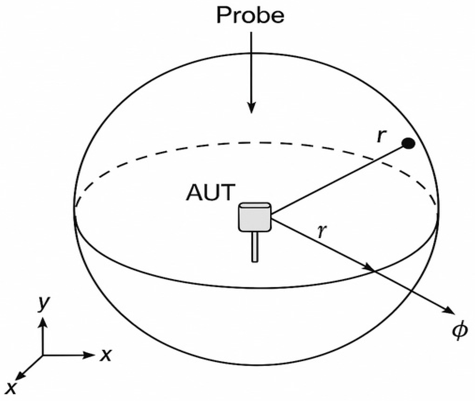
Figure 4 illustrates the setup for measuring near-field electromagnetic radiation emitted by a 5G base station using a spherical coordinate system. The 5G base station antenna, referred to as the Antenna Under Test (AUT), is positioned at the center of the spherical space and acts as the radiation source. A measurement probe is placed on the surface of this hypothetical sphere to detect the electric field strength at a radial distance r. In this coordinate system, r denotes the distance from the antenna to the probe, θ represents the elevation (or polar) angle measured from the vertical axis, and ϕ—although not shown—typically indicates the azimuthal angle around the z-axis. The Cartesian axes (x, y, and z) are included to correlate spherical coordinates with actual spatial directions. The radiation pattern is illustrated with arrows showing the general direction of wave propagation. This configuration is used to assess electromagnetic field levels in the near-field zone, allowing for the spatial mapping of electric field strength E based on the angular position and distance, which aids in analyzing the antenna’s performance.

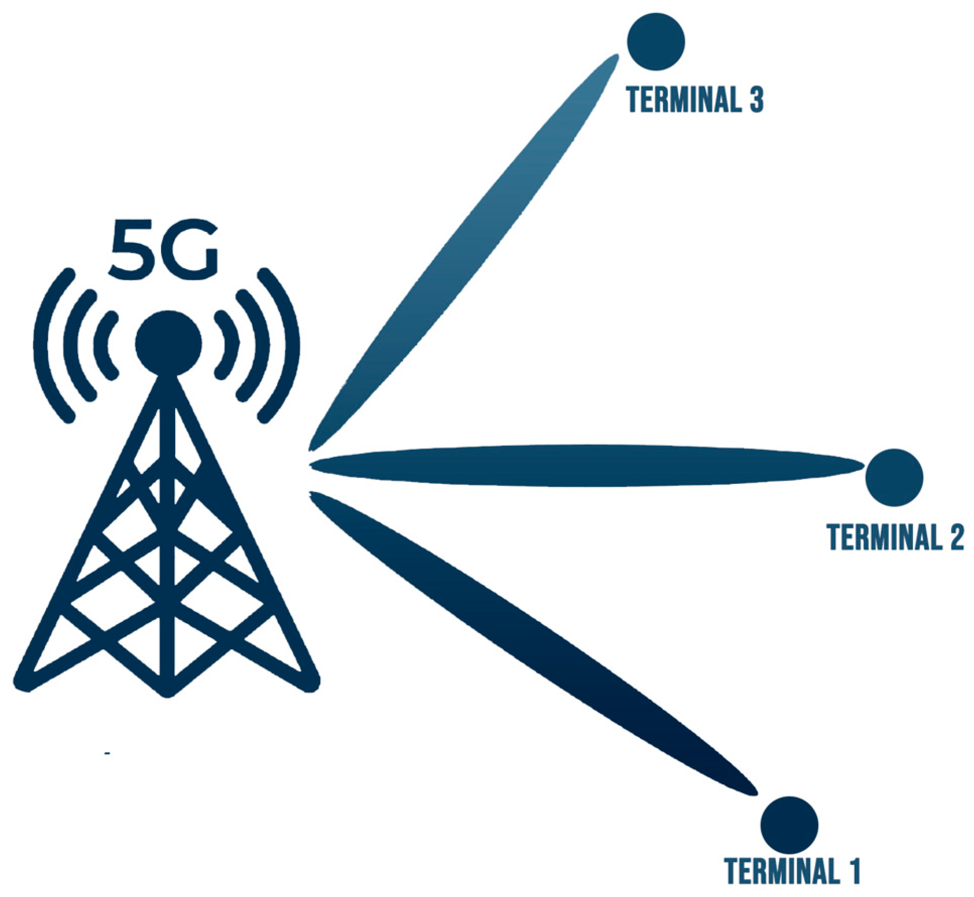
One of the main challenges to the rollout of 5G new radio (NR) is the extensive application of technological innovations like massive MIMO (multiple-input and multiple-output) and beamforming.

The electric field in the distant field near 5G base stations shown in Figure 2 can be determined using the following [27,28,29].

$$E=\sqrt{377{\displaystyle \frac{P_T{G}_T(\theta ,\varphi )}{4\pi R^2}}},$$

(1)

E is the electric field intensity (in volts per meter, V/m). P_T is the transmitted power (in watts). $G_T\left(\theta ,\varphi \right)$ is the gain of the transmitting antenna in the direction $(\theta ,\varphi )$. R is the distance from the antenna to the observation point (in meters). The value of 377 is the intrinsic impedance of free space (η₀ = 377 Ω), and 4πR² represents spherical spreading in free space.

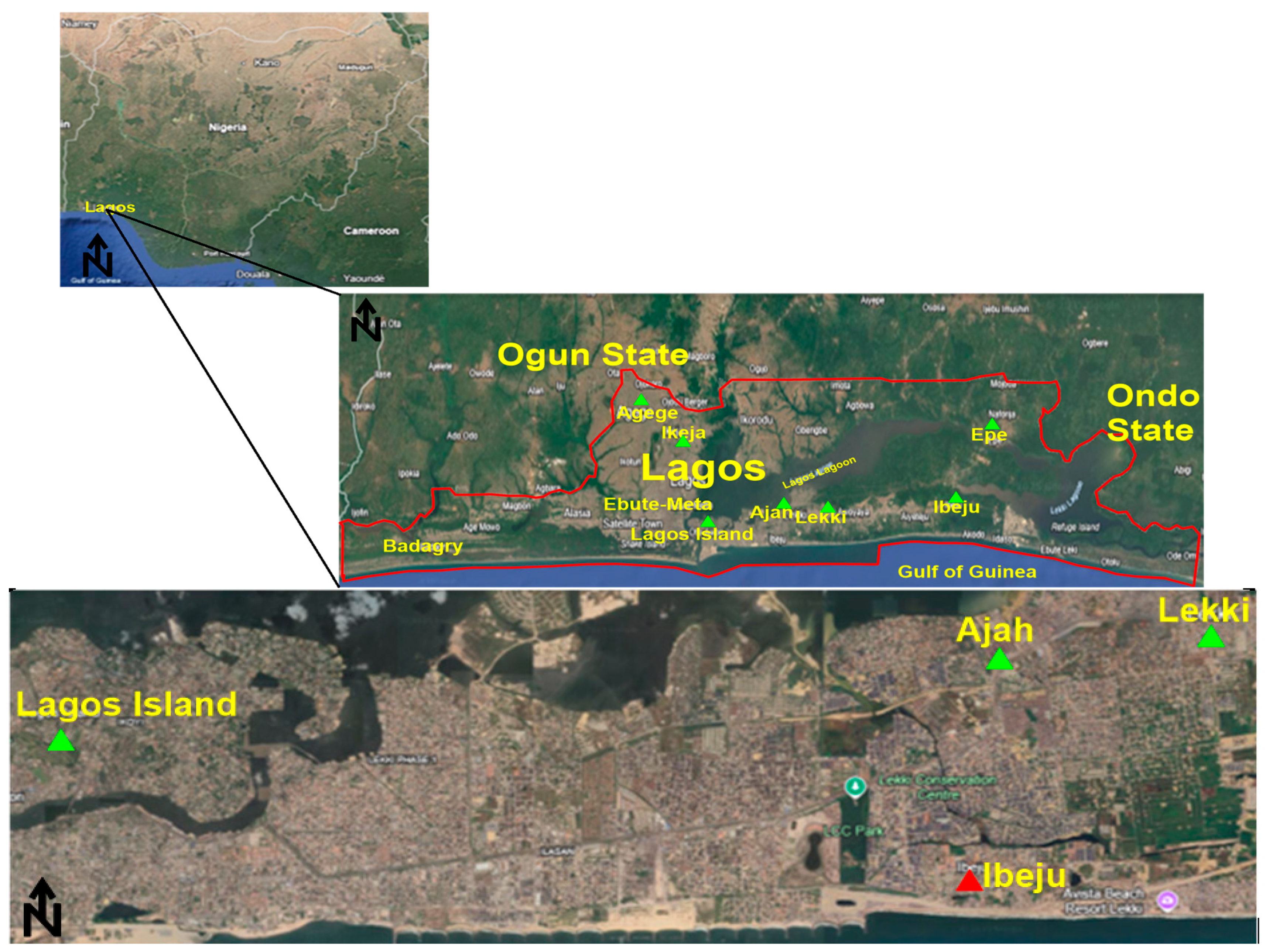
This section presents the method used for the environmental monitoring of electromagnetic radiation at 5G base stations. Measurements were conducted at multiple 5G base stations across six regions in Lagos, Nigeria: Ikeja, Lagos Island, Ikoyi, Lekki, and Ajah. Furthermore, three major operators—MTN, Global Communication, and Airtel—are active in these areas. The active bands of the 5G base stations are shown in

Table 1. Network providers of 5G base stations with individual active bands.

Network Operator	Frequency (MHz)
MTN	35,000
Globalcom	32,000
Airtel	26,000

.

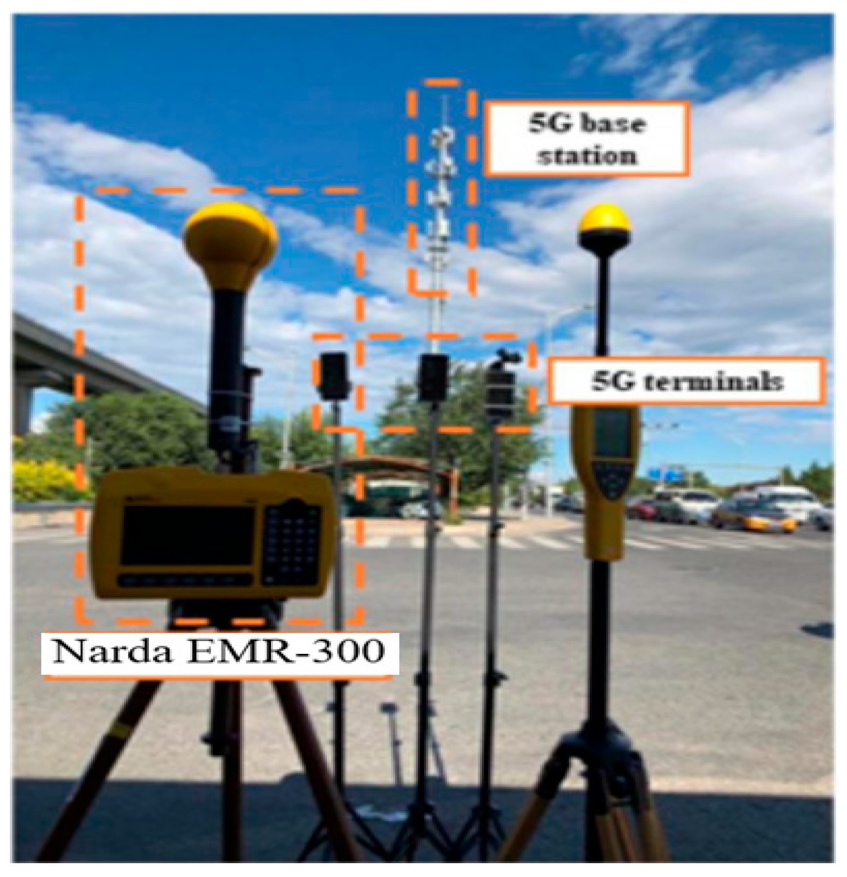
The 5G base station measurement data for the Lekki region is presented in Figure 3. We used the PMM (Narda) EMR-300 (Narda, Pfullingen, Germany), a frequency-selective radiation meter, as our testing device. This equipment was chosen for its ability to monitor the frequency range within the probe’s response. This capability enables the device to accurately capture and display electromagnetic radiation from 5G base stations, showing the spectrum distribution of contributions across different frequencies. SRM-3006 (Narda, Pfullingen, Germany), offers a typical instrumental accuracy of ±1.5 dB across most of its operating range. For highest confidence, careful calibration, spatial resolution, and environmental control are essential to minimize total uncertainty and improve model-matching reliability. Furthermore, measurement accuracy depends significantly on the probe used: Isotropic E-field probes (e.g., EF 0691, EP-601(Narda, Pfullingen, Germany),) offer omnidirectional sensitivity, which is crucial for averaging over three spatial axes. Probe calibration contributes an uncertainty of around ±1.0 to ±1.5 dB, and the expanded uncertainty (combined, 95% confidence level) is ±2.5 to ±3.5 dB. This total uncertainty range is incorporated as an error band when interpreting how well measurements align with theoretical computation. Probe loading and size (relative to wavelength) affect the accuracy; this is minimized by using near-field-compatible small-aperture probes.

2.2. Random Forest Regression Method

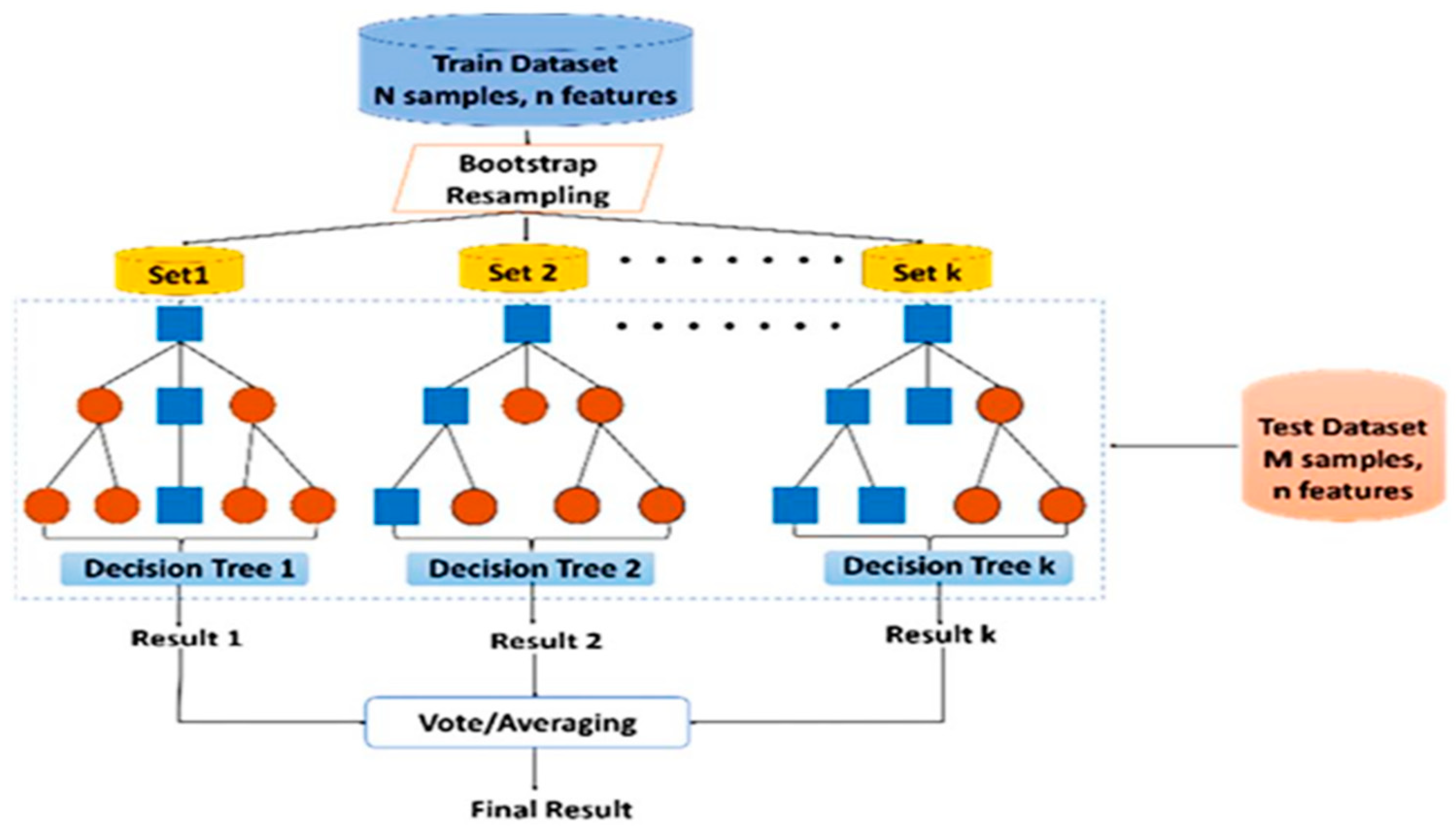
Ensemble learning is a common technique that involves combining multiple learners to improve the performance of a machine learning model [29,30,31,32,33,34,35]. This approach is often divided into two categories based on whether the base learners are generated simultaneously or sequentially. The random forest regression model, which is based on the Bagging (bootstrap sampling) algorithm, exhibits the characteristics of a traditional parallel ensemble learning model, such as randomness in both feature selection and training set composition. Figure 5 illustrates the architecture. In random forest, bootstrapped datasets are created by randomly selecting samples from the training set with replacement, and these datasets are used to train multiple tree learners. The size of each bootstrapped dataset matches that of the original training set. Furthermore, instead of splitting nodes using all available attributes, decision trees in the random forest are constructed using random subsets of the features. A regression decision tree, which is built by partitioning the feature space into subgroups based on a set of splitting criteria, acts as the base learner for the random forest regression model. The training set D is represented by the following equation.

$$\mathit{D}=\{\left({\mathit{x}}_1,y_1\right),\left({\mathit{x}}_2,y_2\right),\dots \left({\mathit{x}}_N,y_N\right)\},$$

(2)

Each data point in the training set is represented by x_i, where x_i is a feature vector (e.g., a set of measurements or attributes), and y_i is the corresponding label or outcome associated with x_i (e.g., the classification or predicted value). For example, in a dataset of weather data, x_i could represent features like temperature and humidity, while y_i could correspond to a label indicating whether it rained (yes or no) that day. i = 1, 2, …, N, where N is the total number of data points in the training set. ${\mathit{x}}_i=\left(x_i^1,x_i^2,\dots ,x_i^n\right),$ where ${\mathit{x}}_i$ denotes the feature vector, and n represents the number of features.

To generate multiple training sample sets, data is randomly sampled from the original dataset D using the Bagging (bootstrap sampling) method. For each training sample set, a Classification and Regression Tree (CART) is constructed using the node random splitting technique, and the least mean square error principle is applied.

For any partition feature j corresponding to a partition node s, the dataset is divided into two subsets, ${\mathit{R}}_1$ and ${\mathit{R}}_2$. The partition feature j is determined by minimizing the mean square errors of ${\mathit{R}}_1$ and ${\mathit{R}}_2$, as well as the sum of these errors. The following are the resulting expressions:

$$\underset{j,s}{\min }[\sum _{{\mathit{x}}_{\mathit{i}}\mathit{ϵ}{\mathit{R}}_1(j,\mathit{s})}{\left(y_i-{\mathit{C}}_1\right)}^2+\sum _{{\mathit{x}}_{\mathit{i}}\mathit{ϵ}{\mathit{R}}_2(j,\mathit{s})}{\left(y_i-{\mathit{C}}_2\right)}^2],$$

(3)

$${\mathit{C}}_1={\displaystyle \frac{1}{{\mathbb{N}}_1}}\sum _{{\mathit{x}}_{\mathit{i}}\mathit{ϵ}{\mathit{R}}_1(j,\mathit{s})}{y}_i,$$

(4)

$${\mathit{C}}_2={\displaystyle \frac{1}{{\mathbb{N}}_2}}\sum _{{\mathit{x}}_{\mathit{i}}\mathit{ϵ}{\mathit{R}}_2(j,\mathit{s})}{y}_i,$$

(5)

${\mathit{R}}_1=\left\{x|x_i^{\left(j\right)}\le s\right\}$ and ${\mathit{R}}_2=\left\{x|x_i^{\left(j\right)}>s\right\}$ are the split areas. Following the division of the feature space into M areas (${\mathit{R}}_1$, ${\mathit{R}}_2$,..., ${\mathit{R}}_M$), the process is repeated for each split area until the stop criterion is met. ${\mathit{C}}_{\mathbf{1}}$ and ${\mathit{C}}_{\mathbf{2}}$ represent the optimal output values of the two areas, respectively, and ${\mathbb{N}}_{\mathbf{1}}$ and ${\mathbb{N}}_{\mathbf{2}}$ are the number of samples in datasets ${\mathit{R}}_1$ and ${\mathit{R}}_2$, respectively. Consequently, a regression tree is designed as

$$f(x)=\sum _{m=1}^M{\mathit{C}}_{m}I(x\in {\mathit{R}}_m),$$

(6)

where the following equation provides the indicator function.

$$I=\left\{\begin{array}{c}1, if(x\in {\mathit{R}}_m)\hfill \\ 0, if(x\notin {\mathit{R}}_m)\hfill \end{array}\right.,$$

(7)

The estimated value can be determined by identifying the leaf node that corresponds to the input features of the instantaneous electric field intensity to be estimated when they are fed into the regression decision tree model.

As a result, the algorithm is robust and exhibits strong fault tolerance, making it well-suited for scenarios where electromagnetic radiation from 5G base stations fluctuates significantly based on operating conditions.

2.3. Dataset

We adopt a two-pronged approach to feature selection, considering both the actual measured values and the principles of electromagnetic radiation to avoid dimensionality issues and overfitting caused by irrelevant features. We carefully select the parameters to be used as inputs and outputs for the random forest regression model, as listed in

Table 2. The random forest regression model’s input and output.

Parameter	Description	Feature
G	Antenna gain	Input
R	Distance between base station and terminal	Input
P	Antenna transmit power	Input
C	The intricacy of the surrounding environmental situations for the base station	Input
N	Number of terminals	Input
TSM	Terminal service mode	Input
E	Average electric field intensity over 6 min	Output

. The measurement campaign is conducted on both weekends and weekdays.

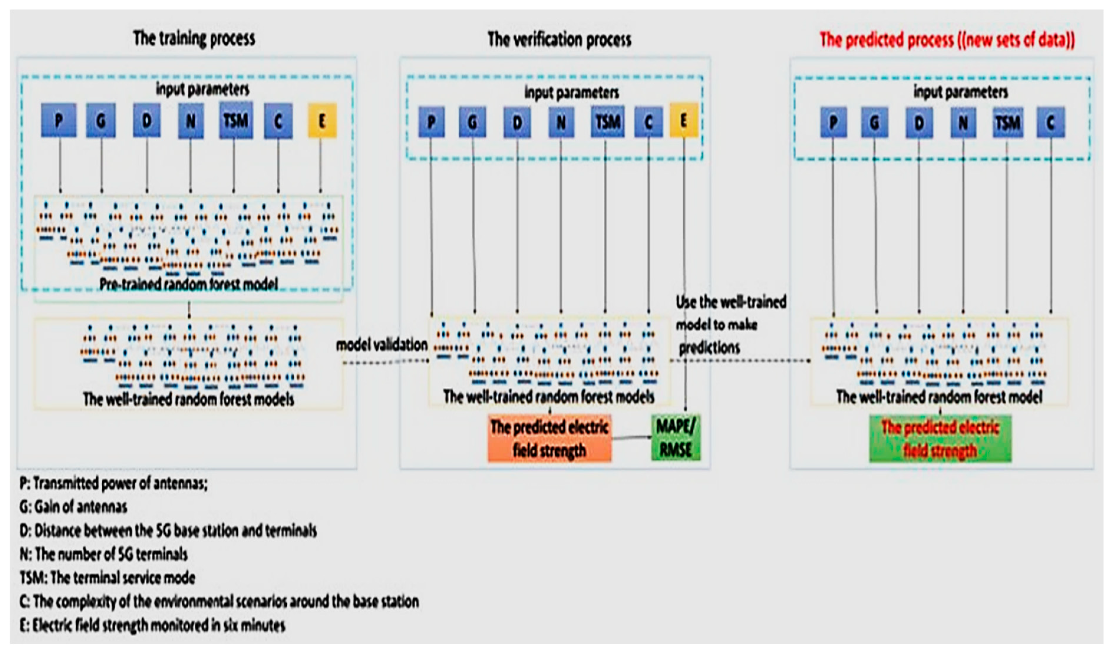
The training, validation, and prediction processes of the random forest model are illustrated in Figure 6. The random forest algorithm was developed using Python 3.12.0, with implementation carried out through the scikit-learn library. During the training phase, the dataset includes inputs such as the antenna’s transmission power, antenna gain, terminal service modes, the number of 5G terminals, the distance between 5G terminals and the base station, the environmental complexity around the 5G base station, and the monitored electric field intensity. This dataset is used to train the pre-trained random forest model, resulting in a well-trained model. In the validation phase, the same set of inputs—antenna transmit power, antenna gain, terminal service modes, number of 5G terminals, distance from 5G terminals to the base station, environmental complexity, and monitored electric field intensity—are used. The output of the model is the predicted electric field intensity, and by comparing the predicted and monitored values, the error’s MAPE (Mean Absolute Percentage Error) and RMSE (Root Mean Squared Error) are calculated. In the prediction process, the dataset (new data) includes inputs such as the antenna’s transmit power, antenna gain, terminal service modes, the number of 5G terminals, the distance between the terminals and the base station, and the environmental complexity surrounding the 5G base station. The trained random forest model receives these input parameters and automatically predicts the electric field’s intensity.

Selecting the right features is the first step in accurately estimating electromagnetic radiation levels. As shown in Equation (1), factors such as antenna transmit power (P), antenna gain (G), and the distance (D) from the 5G base station significantly influence the electric field radiation level. In practice, three major Nigerian network operators—MTN, Globalcom, and Airtel—use a specific type of transmitting antenna to service the terminal.

Table 3. Transmission power at various locations.

Site	Base Station	Gain (dBi)	Transmission Power (W)
1	BTS5A23	23.46	221
2	A9921B X28	17.93	250
3	BS6712	24.47	125
4	BTS6C22	17.93	339
5	A9941B X28	23.46	221

provides details on the nominal values of antenna transmit power for each operator. While there may be slight variations between these nominal values and the actual transmit power in certain monitoring conditions, this difference does not impact the accuracy of our predictions. The gain (absolute gain) is represented as a dimensionless ratio of the power output in a specific direction to the power radiated by the reference antenna. The model’s ability to predict the strength of the electromagnetic radiation field is not solely reliant on these variables; instead, it performs a comprehensive analysis using multi-dimensional data. As illustrated in Figure 2, the monitoring point is equipped with a terminal, and the antenna beam is specifically designed to serve this terminal. Therefore, the gain referred to here is the nominal gain (P) of the antenna. Beamforming adjusts the radiation direction of antennas, concentrating wireless signals in a specific direction rather than radiating them uniformly, which results in a higher gain value for the antenna.

Just as the distance (D) between the 5G base station and the measurement site influences the measured electric field intensity, D is also selected as an input parameter.

A higher observed electric field intensity results from multiple beam overlaps caused by a concentration of 5G terminals. Therefore, we believe that the number of terminals has a significant impact on the detected radiation level from the 5G base station. In the measurement, we increase the number of 5G terminals from 1 to 4 to represent a more typical scenario. By analyzing monitoring data from selected areas in Lagos, Nigeria, we observe that as the number of terminals increases, the monitoring field strength also rises (

Table 4. The intensity of the electric field increases as the number of terminals increases.

Number of Terminal	Station 1 (Lekki Region)	Station 2 (Lagos Island Region)	Station 3 (Ajah Region)
1	0.998	0.474	0.196
2	1.014	1.896	1.546
4	2.411	4.477	4.354

Measurements are in V/m.

). Given its importance to the outcome, the number of terminals is one of the key features included in our model.

In practice, the antenna transmit power varies as the terminal service modes change. Therefore, it is important to consider both the impact of terminal service modes on transmit power and the effect of antenna transmit power on the level of electromagnetic radiation. An analysis of monitoring data from selected areas in Lagos reveals that the electric field intensity changes with different terminal service modes (

Table 5. The intensity of the electric field changes with the TSM.

TSM	Station 1 (Lekki Region)	Station 2 (Lagos Island Region)	Station 3 (Ajah Region)
Data transmission	2.810	3.147	1.556
Voice communication	0.451	0.498	0.336
Video call	0.633	0.701	0.394

Measurements are in V/m.

). The data transmission mode results in significantly higher electric field intensity compared to voice communication, with different service modes corresponding to varying data transmission rates (

Table 6. Variation of electric field intensity and data transmission rate across different terminal service modes.

TSM	E-Field Intensity (V/m)	Rate of Transmission (Mbps)
Data transmission	2.810	1170.64
Voice communication	0.451	650.12
Video call	0.633	820.73

). As a result, we have included the 5G terminal service mode (TSM) as a feature in our model.

Data for our model was collected from 52 base stations across various regions of Lagos, Nigeria. These base stations are situated in diverse environments, ranging from busy streets to remote suburbs. To account for the potential reflections and diffractions caused by nearby buildings on test site results, we included environmental variables as inputs, considering both line-of-sight (LOS) and non-line-of-sight (NLOS) transmission scenarios. Consequently, the complex surrounding environment of each 5G base station (C) became a key characteristic. Lagos, Nigeria, experiences two primary seasons: the wet and dry seasons. Prior studies [32,33] have shown that atmospheric refractivity is higher during the wet season compared to the dry season, making the wet season the worse atmospheric period for analysis. Therefore, the RF measurement campaign was conducted in August 2024, at the height of the rainy season, to capture the effects of atmospheric attenuation. The height of the base station is 60 m according to the service providers, while the height of the receiving station is maintained at 1 m throughout. The measurements were taken at a distance ranging from 0.5 m to 3 m away from the base station.

The level CCC (climate change commission) in the document, as produced by the Lagos State Ministry of Environment [34], represents the environmental complexity surrounding the base stations. It is categorized into three levels, 1, 2, and 3, which correspond to dense urban areas, urban regions, and suburban areas, respectively. The primary criterion for determining CCC is the building density, while the secondary criterion is the population density around the base stations. Building density is defined as the ratio of the building coverage area to the total area, represented by a circle centered at the base station, with the radius being the distance from the base station to the monitoring point. The population density map helps clarify the population distribution and allows for easy differentiation between densely urban, urban, and suburban areas.

We have established the calculation procedures for CCC based on the principles outlined in the “Lagos Master Plan” as follows:

• Dense urban areas are defined as regions where building coverage exceeds 70% of the total area or where the population density is greater than 20,000 people per square kilometer. The entire area is defined by a circle with the base station at its center and the radius being the distance between the base station and the monitoring point.
• Suburban areas are characterized by having less than 50% building coverage of the total area or a population density of 7000 or fewer people per square kilometer.
• The remaining areas are classified as urban areas.

2.4. Estimation of Frequency-Selective Signal Field Strength

Lekki is a narrow stretch of land situated between two major bodies of water: the Atlantic Ocean to the south, known for its sandy beaches, and the Lekki and Lagos Lagoons to the north, which form its natural northern boundary. This positioning gives Lekki a long, strip-like shape, extending roughly from the east to the west. The urban development in Lekki follows a linear pattern centered around the Lekki-Epe Expressway, which acts as the main transportation route. The region is divided into phases (like Lekki Phase 1 and 2) and various residential estates, resulting in a grid-based street network radiating from the main road. The topography is mostly flat and low-lying and only a few meters above sea level, making it prone to flooding during heavy rainfall or tidal surges. The landscape includes mangroves, swamps, and reclaimed land, with areas like the Lekki Conservation Centre helping to protect the region’s biodiversity and wetlands.

Lagos Island is a compact, naturally formed island with an irregular coastline, and it is surrounded by Lagos Lagoon, Five Cowrie Creek, and other waterways. It has high-density urban structures, blending residential, commercial, and historical areas. The road layout combines planned grid patterns and organic street designs, especially in older neighborhoods. Like much of Lagos, the island is flat and close to sea level. It is well-connected to surrounding districts via key bridges such as the Carter Bridge, Eko Bridge, and Third Mainland Bridge, reflecting a mix of natural geography and intensive urban development.

Ajah is shaped by its coastal, linear layout, running along the Lekki-Epe Expressway, with growth patterns that reflect both planned estates and informal expansion. The area is flat and low-lying and bordered by creeks and lagoons, which contribute to its partially fragmented, organically growing form. Ajah’s development is influenced by nearby wetlands and water bodies, resulting in a mix of residential sprawl and natural features.

At the millimeter-wave range, propagation is highly sensitive to material properties around the base station, with strong attenuation through the walls, glass, and trees; it behaves almost like line-of-sight propagation. Common materials found around the study areas are dry concrete, brick, glass (window), dry and wet asphalt, vegetation, metallic poles ocean (salt water), and fresh water.

Based on the defined inputs and outputs, the dataset for training and evaluating the random forest regression model is derived from the measured results of 52 base stations. The dataset consists of 1344 measured data points, which are randomly split into two parts: 942 data points (70%) for the training set and 402 data points (30%) for the test set. The random forest regression model is trained using the training set, and the optimal parameters are selected. The performance of the model is assessed using the MAPE and RMSE on the test set as

$$MAPE={\displaystyle \frac{1}{n}}\sum _{i=1}^n{\displaystyle \frac{\left|y_i^{\prime }-y_i\right|}{y_i}},$$

(8)

$$RMSE=\sqrt{{\displaystyle \frac{1}{n}}\sum _{i=1}^n{\left(y_i^{\prime }-y_i\right)}^2},$$

(9)

where $y_i$ is the measured electric field strength in the test set, $y_i^{\prime }$ is the estimated electric field strength, and n is the number of data points in the test set.

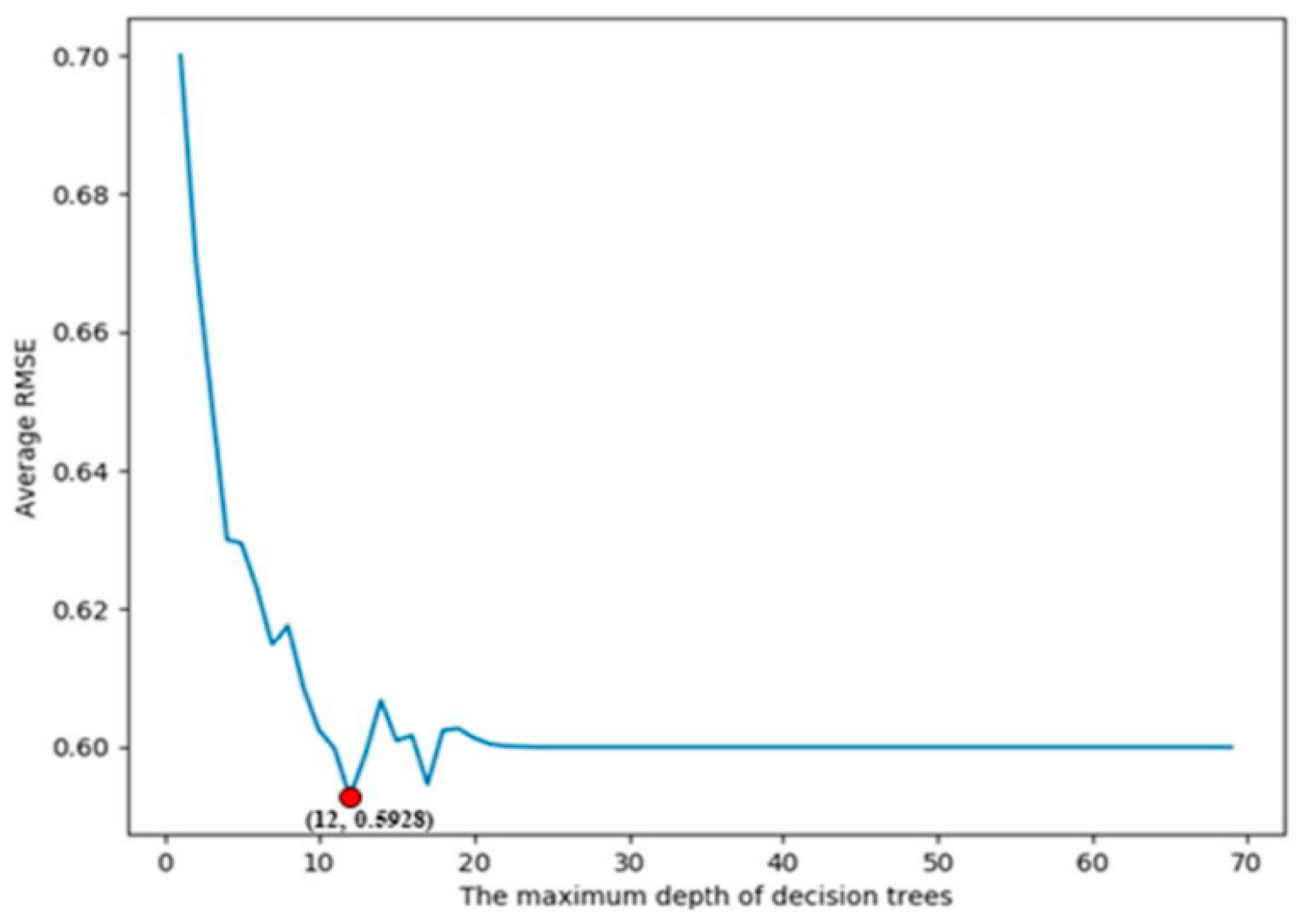
The maximum depth of decision trees (D), the number of decision trees (${\mathbb{N}}_1$), and the maximum number of features that can be employed in the creation of decision trees (${\mathbb{N}}_2$) are the three key parameters of the random forest regression model. The maximum depth of decision trees is used to limit the depth of decision trees when the model with many features is trained with a small amount of data. This helps prevent the model from becoming overly complex and from underperforming in terms of generalization. The complexity and ability of the model to capture relationships are primarily influenced by the number of decision trees. The differentiation between decision trees depends largely on the maximum number of features used during the development process. The optimal values for these parameters can be determined using ten-fold cross-validation [25,36,37]. In this method, the dataset is randomly divided into ten subsets, with each subset used once as the validation set, and the validation process is repeated ten times, in line with the ten-fold cross-validation approach.

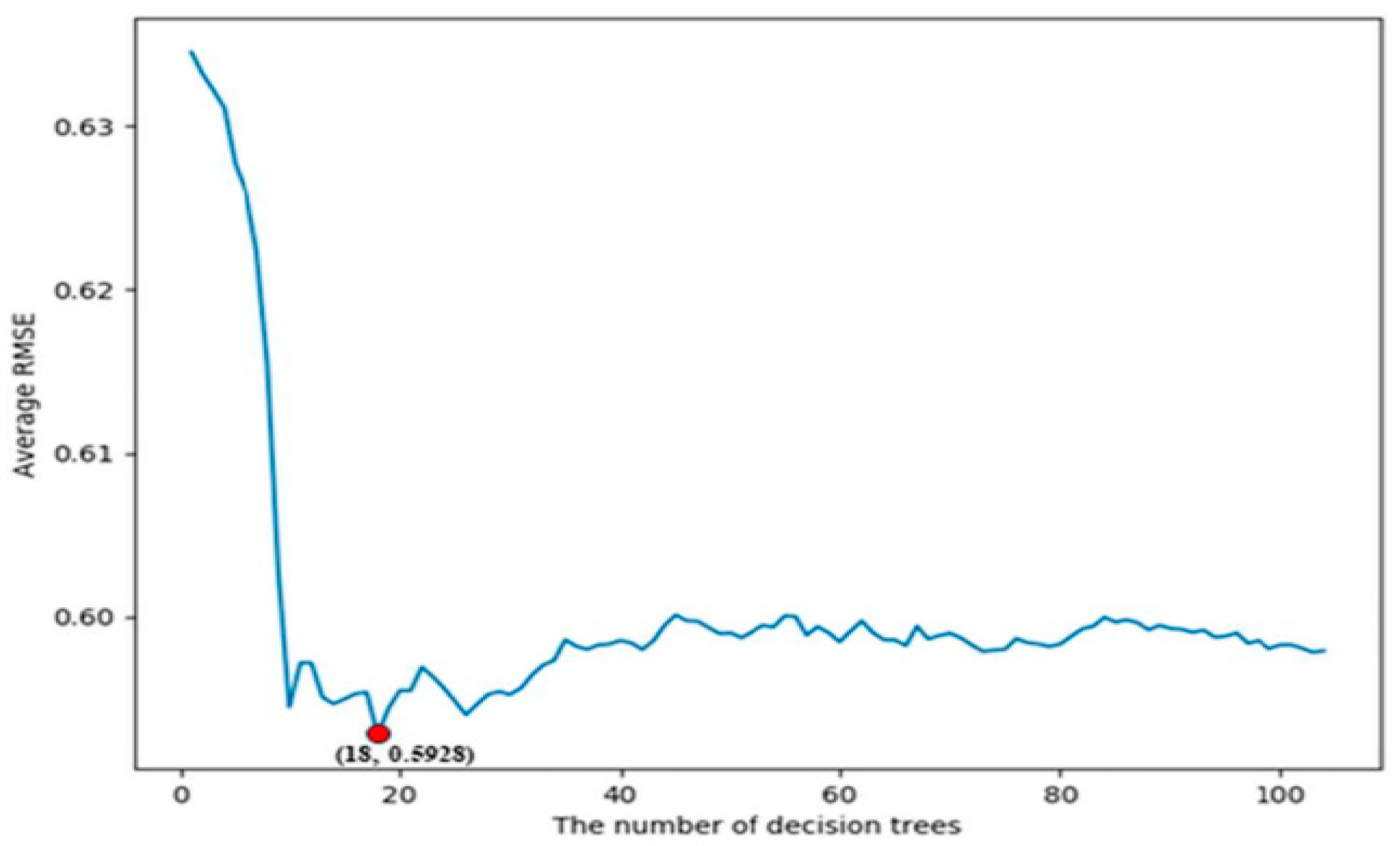
The entire model training process was conducted using an 8th Generation Intel Core i7 processor, 16 GB of RAM, a 64-bit operating system, and a 1 TB hard drive, with Python as the development software and Scikit-learn 0.24.1 as the framework. The model took approximately 3821.6 s, or 1.06 h, to complete training. To assess the real performance of the machine learning model with various parameters, we averaged the MAPE and RMSE across ten validation sets. Through this evaluation, we determined the values of D, ${\mathbb{N}}_1$, and ${\mathbb{N}}_2$ to be 12, 18, and 3, respectively. Specific parameters and settings for the random forest regression model are provided in

Table 7. Setups and parameters for the random forest regression model.

Parameter	Definition	Value
${\mathbb{N}}_1$	Number of decision tree	18
${\mathbb{N}}_2$	Maximum number of features allowed to be employed in decision tree design	3
D	Maximum depth of decision trees	12

.

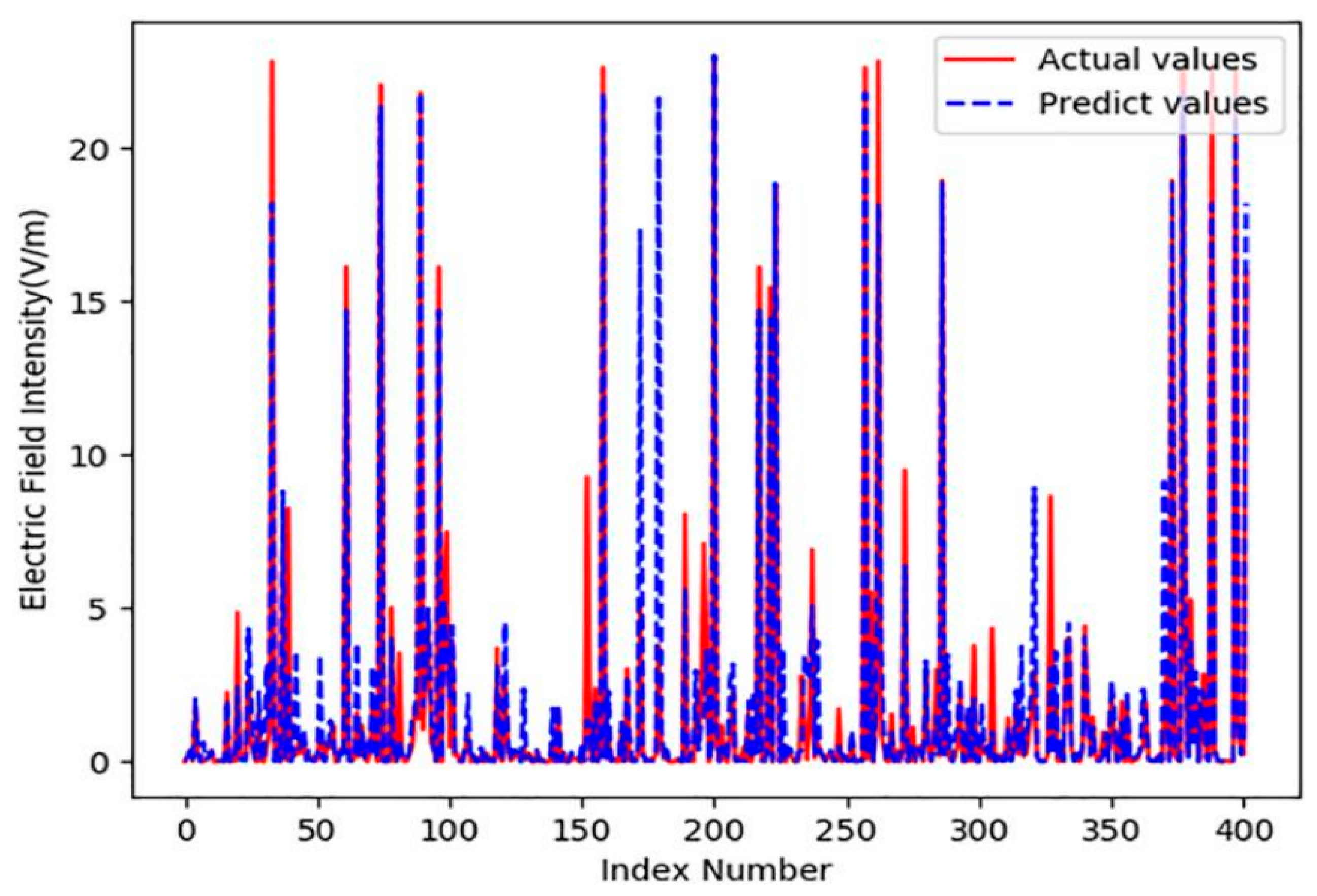
Using the random forest regression model with the optimal settings mentioned above, Figure 7 presents a comparison between the estimated electric field strength and the measured values, with index numbers ranging from 1 to 404 in the test set. According to Figure 8, the predicted values appear to be consistently lower than the measured ones in regions where the field strength is high. For instance, Figure 7 shows that estimation errors can reach around 5 V/m. Such discrepancies could mean the difference between a measurement point complying with safety limits or not. This highlights the importance of conducting on-site measurements to ensure accurate compliance verification. 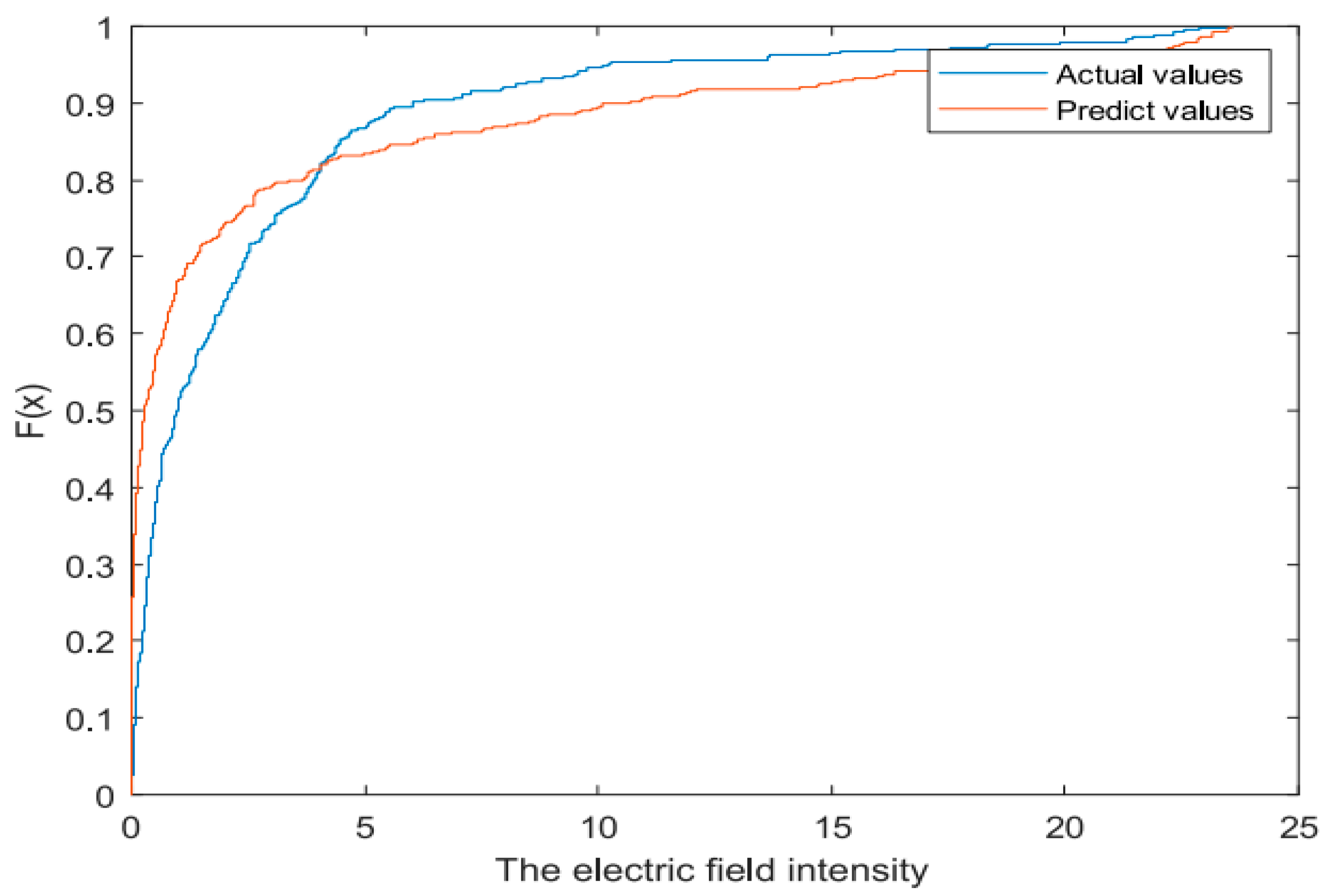Figure 8 compares the measured values with the predicted values in the CDF plots of electromagnetic fields. The results indicate a strong agreement between the estimated and measured electric field intensities at different locations. Any observed discrepancies are likely due to occasional interference in the measurement environment, such as the presence of other 5G terminals or urban railroads, which were not considered in the estimation process. Additionally, we calculated the Root Mean Square Error (RMSE) and Mean Absolute Percentage Error (MAPE) to evaluate the performance of the estimation method. The results revealed an RMSE of 0.5928 and an MAPE of 5.985%. These findings further validate the effectiveness and reliability of the estimation technique. The proposed model is capable of accurately estimating the radiation field intensity of 5G base stations by considering a broad range of factors that influence electromagnetic radiation, thanks to its comprehensive analysis of multi-dimensional data.

3. Results and Discussion

This section provides a discussion on the parameters and behavior of the random forest algorithm.

3.1. Number of Decision Trees and Their Maximum Depth

Figure 9 illustrates the relationship between the average RMSE from ten-fold cross-validation and the number of decision trees, with the maximum depth of decision trees (D) set to 12 and the maximum number of features set to three. Initially, the RMSE is high due to the low complexity of the machine learning model, but it rapidly decreases as the number of decision trees increases. While there are occasional fluctuations, the RMSE generally shows a downward trend before slightly rising as the number of decision trees increases. The model achieves its best performance and lowest RMSE when the number of decision trees is set to 18. Overfitting can occur when a model with a large number of decision trees is trained on a small dataset, leading to an increase in RMSE. If the number of decision trees exceeds 18, further increases in the number of trees and computation time will not lead to a reduction in RMSE (Figure 10).

By limiting the maximum depth of decision trees, we were able to prevent overfitting in the random forest regression model used to estimate the electric field intensity around 5G base stations. As shown in Figure 11, both the number of decision trees and the maximum depth of the trees have a similar impact on the model’s performance. Initially, as the maximum depth of the decision trees increases, the RMSE decreases. However, after a certain point, the RMSE begins to rise again. Through analysis, we determined that a maximum decision tree depth of 12 yields the lowest RMSE (0.5928). The relationship between RMSE and parameter values can help guide the selection of optimal key parameters for a machine learning model.

3.2. Proposed Model Against Theoretical Calculation

It is important to highlight the advantages of our methodology, as described using Equation (1) in Section 2.1, for directly evaluating exposure. To compare the theoretical results obtained through Equation (1) with the monitoring data, we selected two types of sites: LOS (line of sight) and NLOS (non-line of sight). The theoretical calculations yield significantly higher values because the nominal power is used in place of the actual antenna transmitting power in the calculations based on Equation (1). Our model incorporates four terminal devices as input parameters, and to optimize the prediction, the data transmission mode is selected for the terminal service mode.

Table 8. Proposed model versus theoretical computation.

	E-Field Intensity (V/m)			MAPE (%)
Index of Site	Measurement	Equation (1)	Proposed Model	Equation (1)	Proposed Model
1	2.31	13.21	2.51	473	6.01
2	1.75	8.81	1.89	431
3	1.48	11.41	1.53	725
4	2.17	21.17	2.35	923

presents the comparison results, with Sites 1 and 2 being LOS sites and Sites 3 and 4 being NLOS sites.

We review the results obtained earlier. Equation (1) is expected to provide a reasonably accurate estimation of the electromagnetic (EM) field levels in LOS conditions. Since the nominal power of the base station is higher than its actual transmission power, which varies depending on the terminal’s different statuses, the computed value from Equation (1) is considerably higher than the measured value. To address variations in transmission power, our model incorporates the number of terminals and terminal services as input parameters. By accounting for these factors, the proposed approach bridges the gap between theoretical calculations and real-world measurements, offering more accurate and realistic estimations of EM field levels.

Equation (1) does not incorporate the presence of multiple propagation channels, such as direct, reflected, and diffracted paths, between the base station and the test point in our scenarios, and it only considers the direct path in NLOS situations. As a result, Equation (1) does not provide sufficient information to accurately assess the method’s performance in NLOS locations, especially in dense environments with complex propagation channels, where performance is likely to be significantly affected. Consequently, the error in Equation (1) is larger in NLOS scenarios. In contrast, the proposed model accounts for environmental complexity, allowing it to incorporate the multipath effect. By integrating these factors, our model provides more accurate and reliable estimations of EM field levels in NLOS conditions. The inclusion of multipath effects and environmental factors in our model mitigates the limitations of Equation (1), leading to improved performance in estimating EM field levels in NLOS sites.

3.3. Proposed Method Against Various Machine Learning Algorithms

This subsection assesses the performance of different machine learning models in estimating the electric field strength of 5G base stations, including linear regression (LR), back-propagation neural networks (BPNN), and random forest regression models.

A linear regression model, a basic machine learning technique, can automatically determine the optimal coefficients for the fitting function by minimizing RMSE during the training process. For the BPNN model, three key parameters are critical: the number of hidden layers, the number of nodes in each layer, and the learning rate. The learning rate plays a significant role in adjusting the step size for parameter updates in the BPNN. A high learning rate could cause the model to skip over optimal values, while a low learning rate might slow down the training process. To ensure that optimal parameter values are not missed, the learning rate is set to 0.001. Based on the prior ten-fold cross-validation discussion, three hidden layers are chosen, with the optimal number of nodes in each layer being 10, 8, or 2.

Table 9. The various machine learning models’ parameter settings.

Machine Learning Approach	Setting of Parameter	Time (s)
BPNN	MLPRegressor(HiddenLayerSizes = (10, 8, 2), LearningRate = 0.001)	3962
Linear regression	LinearModel.LinearRegression ()	26.48
Random forest regression	RandomForestRegressor (${\mathbb{N}}_1=100, {\mathbb{N}}_2=5, D=19)$	3822.7

outlines the parameter settings for all machine learning models.

A comparison is conducted between the values predicted by various machine learning models and the actual values.

Table 10. The RMSE and MAPE of various machine learning methods.

Machine Learning Method	RMSE	MAPE (%)
BPNN	1.2192	11.95
Linear Regression	2.8198	64.69
Random Forest Regression	0.5930	6.99

presents the MAPE and RMSE for the different machine learning models.

It is evident that, compared to other models, the random forest regression model provides more accurate estimates of electric field intensity near 5G base stations, as indicated by its lower MAPE and RMSE. The complex relationship between features and electric field strength makes it challenging for a simple linear regression model to achieve accurate estimates. However, the BPNN model, with its multi-layered neurons, is better suited to capturing complex relationships and yields more accurate results than the linear regression model. Despite this, there is still a noticeable difference between the predicted and actual values, even with the BPNN.

The random forest regression model, an ensemble learning approach, utilizes the Bagging algorithm and random feature selection to generate multiple decision trees. The final estimate is derived by averaging the outputs of these decision trees. Unlike single learners such as linear regression and BPNN models, the random forest regression model’s inherent characteristics enhance its generalization ability, making it more resilient to anomalous measurement data. In addition to its suitability for estimating electric field intensity around 5G base stations, the random forest regression model offers further advantages, including support for parallel training and the elimination of costly data preprocessing. Given its superior performance and robustness compared to alternative models, the random forest regression model is highly recommended for the accurate prediction of electric field intensity near 5G base stations. The variation in uplink/downlink frequencies introduces differences in signal propagation and interference, which may influence the model’s ability to generalize across scenarios. This variability can contribute to the observed MAPE of 5.98% and RMSE of 0.5928, especially if higher frequencies with less stable behavior are underrepresented in the training data.

Feature importance analysis in the random forest model highlights the relative influence of each input variable on the predicted electromagnetic radiation levels. This not only enhances interpretability but also supports more focused data collection, better model optimization, and a deeper understanding of key environmental and technical drivers.

Finally, it is important to note that while the model shows good performance, discrepancies between the model’s predictions and real-world measurements could stem from unaccounted external variables (e.g., interference from other base stations or signal reflection in densely built environments). Environments are different from one another, and climatic conditions also vary from one place to another. The dataset used for this work is obtained from Lagos, Nigeria, which is a typical urban setting; the model exhibits quality performance in urban settings, but the degree of accuracy in rural or remote areas could be challenged. Hence, these factors limit the performance of the model’s prediction accuracy but can still provide insights and useful information for 5G cellular network engineers in network planning, management, and optimization.

4. Conclusions and Future Work

In conclusion, this paper presents a novel approach for estimating ground plane radiation intensity around 5G base stations using a random forest regression model. We explored the key characteristics of machine learning in the estimation process. In practice, the proposed method effectively provides accurate electric field intensity estimates at the ground plane given the necessary inputs such as transmit power, antenna gain, distance between the base station and terminal, number of 5G terminals, terminal service modes, and the environmental complexity surrounding the 5G base station. The accuracy of the model is validated by an MAPE of 5.98% and an RMSE of 0.5928. This method can be applied to enhance electromagnetic wave coverage for 5G base stations and improve the precision of electromagnetic radiation level estimates. Communication network engineers can utilize this technique in the design and optimization of cellular networks. However, the data collected may also be influenced by the antenna’s orientation. If the antenna is rotated to a different direction, the individual readings could vary significantly. Alternatively, it may be necessary to shield the antenna’s radiation using different materials, which could be explored in future studies. More specific suggestions for overcoming the current model’s limitations (like addressing antenna orientation or shielding methods) would help guide further research. Expanding the dataset to include data from other regions or considering the dynamic nature of 5G service deployment could provide a more comprehensive outlook.

References

1. Mezzavilla, M.; Polese, M.; Zanella, A.; Dhananjay, A.; Rangan, S.; Kessler, C.; Rappaport, T.S.; Zorzi, M. Public safety communications above 6 GHz: Challenges and opportunity. IEEE Access 2018, 6, 316–329. [Google Scholar] [CrossRef]
2. 5G EMF Surveys. Available online: https://www.gsma.com/publicpolicy/emf-and-health/safety-of-5g-networks/5g-emf-surveys (accessed on 10 October 2024).
3. Chiaraviglio, L.; Lodovisi, C.; Franci, D.; Pavoncello, S.; Aureli, T.; Blefari-Melazzi, N.; Alouini, M.-S. Massive measurements of 5G exposure in a town: Methodology and results. IEEE Open J. Commun. Soc. 2021, 2, 2029–2048. [Google Scholar] [CrossRef]
4. Lee, A.-K.; Jeon, S.-B.; Choi, H.-D. EMF levels in 5G new radio environment in Seoul, Korea. IEEE Access 2021, 9, 19716–19722. [Google Scholar] [CrossRef]
5. Erunkulu, O.O.; Zungeru, A.M.; Lebekwe, C.K.; Chuma, J.M. Cellular Communications Coverage Prediction Techniques: A Survey and Comparison. IEEE Access 2020, 8, 113052–113077. [Google Scholar] [CrossRef]
6. Electromagnetic Field (EMF) Measurements Near 5G Mobile Phone Base Stations. Available online: https://www.ofcom.org.uk/spectrum/electromagnetic-fields/mobile-base-station-audits (accessed on 10 October 2024).
7. Assessment of the Exposure of the General Public to 5G Electromagnetic Waves. Available online: https://www.anfr.fr/fileadmin/mediatheque/documents/5G/20200410-ANFR-rapport-mesures-pilotes-5G-EN.pdf (accessed on 18 August 2024).
8. Aerts, S.; Deprez, K.; Colombi, D.; Bossche, M.V.D.; Verloock, L.; Martens, L.; Törnevik, C.; Joseph, W. In situ assessment of 5G NR massive MIMO base station exposure in a commercial network in Bern Switzerland. Appl. Sci. 2021, 11, 3592. [Google Scholar] [CrossRef]
9. Keller, H. On the assessment of human exposure to electromagnetic fields transmitted by 5G NR base stations. Health Phys. 2019, 117, 541–545. [Google Scholar] [CrossRef]
10. Aerts, S.; Verloock, L.; Bossche, M.V.D.; Colombi, D.; Martens, L.; Tornevik, C.; Joseph, W. In-situ measurement methodology for the assessment of 5G NR massive MIMO base station exposure at sub-6 GHz frequencies. IEEE Access 2019, 7, 184658–184667. [Google Scholar] [CrossRef]
11. Standard EN 62232:2017; Determination of RF Field Strength, Power Density and SAR in the Vicinity of Radio Communication Base Stations for the Purpose of Evaluating Human Exposure. International Electrotechnical Commission (IEC): Geneva, Switzerland, 2022.
12. Report on the Implementation of the Council Recommendation on the Limitation of Exposure of the General Public to Electromagnetic Fields (0 Hz–300 GHz) (1999/519/EC) in the EU Member States, Release 2.1.; Project No. SI2.489570-SANCO/2OO7/C7/06; European Commission’s Directorate-General for Health and Food Safety: Brussels, Belgium, 2008.
13. ICNIRP, Guidelines for limiting exposure to time-varying electric, magnetic and electromagnetic fields (up to 300 GHz). Health Phys. 1998, 74, 494–522.
14. Famoriji, O.J.; Shongwe, T. Simple and effective electromagnetic wave propagation loss model in gsm band for smart campus applications. SSRG Int. J. Electr. Electron. Eng. 2024, 11, 306–311. [Google Scholar] [CrossRef]
15. Famoriji, O.J.; Kashif, R.; Lin, F. Millimeter-Wave Massive MIMO Channel Sounding for Future Mobile Broadband; IEEE International Conference on Ubiquitous Wireless Broadband (ICUWB): Nanjing, China, 2016. [Google Scholar]
16. Federal Office of Metrology METAS, Section Electricity, Measurement Method for LTE Base Stations; METAS-Rep. 2012-218-808, Technical Report; METAS: Bern, Switzerland, 2012.
17. Recommendation ITU-T K.83; Monitoring Field Strengths of Electromagnetic Fields, Document E 36701; Series K: Protections Against Interference. International Telecommunication Union, (ITU): Geneva, Switzerland, 2011.
18. 5G Technology and Human Exposure to RF EMF; document E 42102, Series K: Protections Against Interference; International Telecommunication Union (ITU): Geneva, Switzerland, 2017.
19. Sagar, S.; Dongus, S.; Schoeni, A.; Roser, K.; Eeftens, M.; Struchen, B.; Foerster, M.; Meier, N.; Adem, S.; Röösli, M. Radiofrequency electromagnetic field exposure in everyday microenvironments in Europe: A systematic literature review. J. Expo. Sci. Environ. Epidemiol. 2018, 28, 147–160. [Google Scholar] [CrossRef]
20. Thors, B.; Furuskar, A.; Colombi, D.; Tornevik, C. Time-averaged realistic maximum power levels for the assessment of radio frequency exposure for 5G radio base stations using massive MIMO. IEEE Access 2017, 5, 19711–19719. [Google Scholar] [CrossRef]
21. Thors, B.; Colombi, D.; Ying, Z.; Bolin, T.; Törnevik, C. Exposure to RF EMF from array antennas in 5G mobile communication equipment. IEEE Access 2016, 4, 7469–7478. [Google Scholar] [CrossRef]
22. Safaripour, A.; Asghari, B.; Hajimiri, A. Proximal-field radiation sensors for millimeter-wave integrated radiators. In Proceedings of the IEEE Radio Frequency Integrated Circuits Symposium (RFIC), Philadelphia, PA, USA, 10–12 June 2018; pp. 256–259. [Google Scholar]
23. CENELEC Standard EN 50383; Basic Standard for the Calculation and Measurement of Electromagnetic Field Strength and SAR Related to Human Exposure From Radio Base Stations and Fixed Terminal Stations for Wireless Telecommunication Systems (110 MHz–40 GHz). CENELEC: Brussels, Belgium, 2010.
24. Agiwal, M.; Roy, A.; Saxena, N. Next generation 5G wireless networks: A comprehensive survey. IEEE Commun. Surv. Tutor. 2016, 18, 1617–1655. [Google Scholar] [CrossRef]
25. Famoriji, O.J.; Shongwe, T. Modeling of Coupled Structural Electromagnetic Statistical Concept for Examining Performance Sensitivity of Antenna Array to Distortion at Millimeter-wave. Appl. Sci. 2024, 14, 7111. [Google Scholar] [CrossRef]
26. Xu, B.; Colombi, D.; Joshi, P.; Ghasemifard, F.; Sanjurjo, D.A.; Di Paola, C.; Tornevik, C. A summary of actual maximum approach studies on EMF compliance of 5G radio base stations. In Proceedings of the 6th European Conference on Antennas and Propagation (EuCAP), Madrid, Spain, 27–31 March 2022; pp. 1–5. [Google Scholar]
27. Larab, M.; Benyoubi, F.; Bensetti, M. Study and modeling of the electromagnetic radiation sources based on phaseless of near magnetic fields for power electronic applications. IEEE Trans. Electromagn. Compat. 2024, 66, 34–47. [Google Scholar] [CrossRef]
28. Bogale, T.E.; Le, L.B. Massive mimo and mmwave for 5G wireless hetnet: Potential benefits and challenges. IEEE Veh. Technol. Mag. 2016, 11, 64–75. [Google Scholar] [CrossRef]
29. Moreta, C.E.G.; Acosta, M.R.C.; Koo, I. Prediction of digital terrestrial television coverage using machine learning regression. IEEE Trans. Broadcast 2019, 65, 702–712. [Google Scholar] [CrossRef]
30. Hou, W.; Shi, D.; Gao, Y.; Yao, C. A new method for radio wave propagation prediction based on finite integral method and machine learning. In Proceedings of the 2017 IEEE 5th International Symposium on Electromagnetic Compatibility (EMC-Beijing), IEEE (2017), Beijing, China, 28–31 October 2017; pp. 1–4. [Google Scholar]
31. Mohammadjafari, S.; Roginsky, S.; Kavurmacioglu, E.; Cevik, M.; Ethier, J.; Bener, A.B. Machine learning-based radio coverage prediction in urban environments. IEEE Trans. Netw. Serv. Manag. 2020, 17, 2117–2130. [Google Scholar] [CrossRef]
32. Famoriji, O.J.; Shongwe, T. Path Loss Prediction in the Tropics using Broadcast Signal: A Deep Learning Framework. Int. J. Appl. Eng. Technol. 2024, 6, 1556–1565. [Google Scholar]
33. Famoriji, O.J.; Shongwe, T. Path Loss Prediction in Tropical Regions using Machine Learning Techniques: A Case Study. Electronics 2022, 11, 2711. [Google Scholar] [CrossRef]
34. Lagos Climate Action plan, Second Five Year Plan 2020–2025. Available online: https://moelagos.gov.ng/wp-content/uploads/2021/09/C40-Lagos_Indesign-Document-Full-Report-Revert-2_Update-2.pdf (accessed on 1 February 2025).
35. Zhang, Y.; Wen, J.; Yang, G.; He, Z.; Wang, J. Path loss prediction based on machine learning: Principle, method, and data expansion. Appl. Sci. 2019, 9, 1908. [Google Scholar] [CrossRef]
36. Available online: http://futurecapetown.com (accessed on 1 February 2025).
37. EMR-300 Broadband RF Survey Meter, Datasheet. Available online: www.narda-sts.com (accessed on 1 March 2025).
Figure 1. A typical 5G network architecture.
Applsci 15 07302 g001
Figure 2. Diagrammatic representation of the beam that the 5G base station emits.
Applsci 15 07302 g002
Figure 3. Measurement of the on-site 5G base station in the Lekki region.
Applsci 15 07302 g003
Figure 4. Setup for measuring near-field electromagnetic radiation in various regions.
Applsci 15 07302 g004
Figure 5. The random forest’s architecture.
Applsci 15 07302 g005
Figure 6. Random forest model flow diagram.
Applsci 15 07302 g006
Figure 7. Comparison of the estimated and real numbers.
Applsci 15 07302 g007
Figure 8. EM field cumulative distribution function plots.
Applsci 15 07302 g008
Figure 9. The connection between the number of decision trees and the RMSE of ten-fold cross-validation.
Applsci 15 07302 g009
Figure 10. Map showing the study areas.
Applsci 15 07302 g010
Figure 11. The connection between the maximum decision tree depth and the RMSE of ten-fold cross-validation.
Applsci 15 07302 g011