Energy-Efficient Hybrid PID Control with Exponential Trajectories for Smooth Setpoint Transitions: Applications in Robotics and Aeronautics

Abstract

In this paper, a modification of the classical PID controller scheme for position control is presented. The resulting controller incorporates an exponential trajectory that smoothly guides the system towards the setpoint and a hybrid mechanism to dynamically reset the exponential signal, allowing an adaptive response to discontinuous reference signals. This combination leverages the benefits of exponential trajectories to reduce overshoot and transient oscillations, while the hybrid system ensures robust performance over a wide range of operating scenarios. Among the advantages of the proposed approach, two stand out: (1) significant improvements in energy savings can be achieved in some cases, and (2) closed-loop system performance can be improved even considering poorly tuned PIDs.

1. Introduction

1.1. Motivation

Proportional–integral–derivative (PID) controllers are widely recognized as a fundamental control strategy in industrial and academic applications. Their simplicity, ease of implementation, and effectiveness in a wide range of systems make them a very important tool of control engineering [1]. Despite their strengths, traditional PID controllers often exhibit limitations when applied to systems requiring precise position control, particularly in scenarios involving stringent transient performance requirements such as overshoot reduction and fast settling times [2].

Several modifications to the classical PID structure have been proposed to address these challenges. These include adaptive tuning methods [3], nonlinear PID strategies [4], and hybrid control schemes [5]. However, these approaches often require complex calculations or introduce new challenges such as increased sensitivity to noise or system uncertainties.

The hybrid system for trajectory restoration combines the advantages of continuous and discrete dynamics, allowing a versatile and robust control strategy for discontinuous changes in reference signals. The proposed method is particularly suitable for applications such as robotic manipulators and servomechanisms [6].

In [7], a hybrid control strategy combining model predictive control (MPC) with PID controllers was introduced to improve the performance of supercritical power units. This approach demonstrated significant improvements in response time and energy savings compared to traditional PID methods. In [8], a fuzzy gain programmed PID controller was developed to improve power quality in grid-connected hybrid solar PV and PEM fuel cell systems. The proposed controller effectively reduced total harmonic distortion, demonstrating its potential for improving energy efficiency. In [9], a hybrid optimization approach for energy control in electric vehicle controllers regulating three-phase induction motors is derived. This method improved the energy efficiency and system performance.

Recent developments reflect the increasing integration of intelligent and hybrid methodologies within PID control architectures. In [10], a neuro-fuzzy and robust PID controller is integrated via active filters to enhance performance under uncertain conditions; the neuro-fuzzy component manages transient behavior, while the robust PID ensures steady-state accuracy. In [11], a neural-augmented PID controller based on deterministic learning is applied to robotic manipulators, guaranteeing the stability and convergence of tracking errors under partial excitation conditions. A hybrid controller combining PID/fractional-order PID with neural network tuning via a zebra optimization algorithm is proposed in [12], yielding enhanced robustness and energy efficiency on a two-link robot system. Reference [13] introduces a 3DOF neuro-fuzzy PID strategy for automatic generation control in hydrogen-integrated multi-area power systems, effectively handling nonlinearities and improving frequency regulation.

In [14], a hybrid adaptive PID scheme combining LMS and backpropagation enables real-time gain adjustment, demonstrating high adaptability and robustness, and serving as a foundation for nonlinear extensions. A hybrid control strategy blending PID and model predictive control (MPC) using a fractional-order RAM model is proposed in [15], where MPC refines the PID reference trajectory to enhance overall system response. The work in [16] presents a hybrid PID framework for automated guided vehicles (AGVs), using genetic algorithms (GAs) to optimize controller gains and support vector regression (SVR) to reduce computational complexity. A boundary logic-based hybrid controller combining sliding mode and PID control for underactuated nonlinear cascade systems is proposed in [17], improving performance on complex dynamic tasks. In [18], a hybrid model-data-driven approach was developed for Euler–Lagrange hydraulic systems where a robust nonlinear controller is combined with actor–critic reinforcement learning to manage model uncertainties, supported by Lyapunov-based stability analysis.

Reference [19] introduces the hybrid MFO-WOA optimization algorithm to solve global optimization problems and tune FOPID/PID controllers, demonstrating faster convergence and potential applicability in IoT-integrated scenarios. Finally, [20] proposes a reset control approach to mitigate setpoint regulation issues in motion systems subject to Coulomb and Stribeck friction, achieving asymptotic stability and significant overshoot reduction where classical PID fails due to persistent oscillations.

1.2. Contribution

The main contribution of this paper is to present a modification of the PID controller, incorporating an exponential trajectory to guide the system smoothly towards the setpoint. The exponential signal is dynamically reset by a hybrid control mechanism, allowing the system to adapt to reference changes effectively. This approach offers significant improvements in transient behavior, including a reduction in overshoot, and in some cases also reduces the amplitude of the control signals, which directly translates into energy savings.

It is important to note that the primary objective of this paper is not to propose a new method for tuning PID controller gains but rather to enhance the performance of already designed PID controllers. For this reason, readers are referred to standard textbooks such as [1], where PID tuning methods are discussed in detail.

1.3. Manuscript Organization

The remainder of this paper is organized as follows: Section 2 presents a thorough analysis of the proposed control scheme. Section 3 presents both simulation and experimental results, highlighting the performance improvements achieved over conventional PID controllers. Section 4 discusses important aspects of the proposed control approach. Finally, Section 5 presents the conclusions and outlines potential directions for future research to further enhance the proposed method.

2. Main Results

2.1. PID Controller

The reader is advised that the goal of this paper is not to provide a new approach to tuning PID controller gains but to improve the performance of previously designed PIDs. For that reason, the reader is recommended to consult textbooks such as [1] where PID tuning is discussed in depth. However, for the completeness of this paper, it is important to briefly recall what a PID controller is.

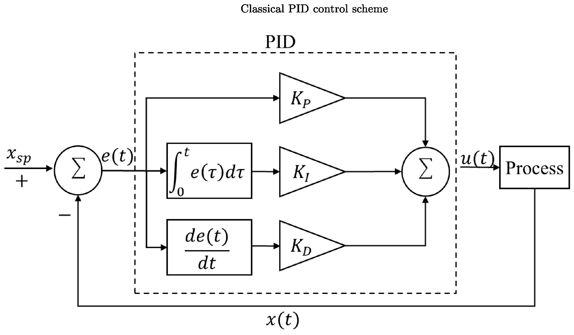
Considering the control scheme depicted in Figure 1, a PID controller is a control law designed to regulate a process variable $x\left(t\right)$, such as position, speed, temperature, or pressure. In order to produce the appropriate control signal $u\left(t\right)$, the PID controller needs the following:

• The error $e\left(t\right)$ at time t, which is the difference between the setpoint and the value of the process variable at the current time t, i.e., $e\left(t\right)=x_{sp}-x\left(t\right)$, where $x_{sp}$ is the desired setpoint, $x\left(t\right)$ is the process variable to be regulated, and $e\left(t\right)$ is the error at time t.
• The integral of the error ${\int }_0^{t}e\left(\tau \right)d\tau$ at instant t.
• The time derivative of the error ${\displaystyle \frac{de\left(t\right)}{dt}}$ at instant t.

The PID controller works as follows: the proportional gain ($K_P$) is responsible for reducing the error $e\left(t\right)$ as quickly as possible by applying a correction proportional to the current error. The integral gain ($K_I$) multiplies the error accumulated over time, i.e., the integral of the error, with the aim of eliminating steady-state errors and ensuring accurate convergence to the setpoint. Finally, the derivative gain ($K_D$) is used to predict future error trends based on the derivative of $e\left(t\right)$, which helps to reduce overshoot and improve system stability. The mathematical expression of the PID is as follows:

$$u\left(t\right)=K_{p}e\left(t\right)+K_i{\int }_0^{t}e\left(\tau \right)d\tau +K_D{\displaystyle \frac{de\left(t\right)}{dt}},$$

(1)

where $u\left(t\right)$ is the control signal produced by the PID.

Notice that the derivative part of the PID controller can be problematic if the measurement of $x\left(t\right)$ is contaminated with noise. To address this issue, an alternative version of the PID controller includes a filter to mitigate the effects of noise on the derivative term. The expression for such a PID controller in the frequency domain is as follows:

$$U\left(s\right)=\left(K_p+K_i{\displaystyle \frac{1}{s}}+K_D{\displaystyle \frac{N}{1+N\frac{1}{s}}}\right)E\left(s\right),$$

(2)

where s is the Laplace variable; $U\left(s\right)$ and $E\left(s\right)$ are the Laplace transforms of the control signal $u\left(t\right)$ and the error $e\left(t\right)$, respectively; and N is referred as the filter coefficient.

Thus, the design of the PID controller involves determining the appropriate gains $K_P$, $K_I$, and $K_D$ and possibly N such that $u\left(t\right)$ induces the desired behavior in the process variable $x\left(t\right)$. Tuning of the PID controller gains can be performed through the approach proposed by Ziegler and Nichols [1,2].

It is important to mention that mathematical software platforms such as MATLAB r2019b with Simulink™ offer powerful automatic control toolboxes that allow PID controllers to be automatically tuned. These toolboxes simplify the design and tuning process by automatically determining the optimal controller parameters to achieve the desired system performance. This capability allows for rapid numerical prototyping and testing of control systems within the simulation environment [21].

2.2. Basic Notions of Hybrid Systems

A hybrid system is a dynamic system characterized by the interaction between a continuous-time process, typically described by differential equations, and a discrete-event system, often modeled using state machines or logical rules [22]. Mathematically, a hybrid system can be described as follows:

$$\left\{\begin{array}{cc}\omega \left(t\right)\in C\hfill & \dot{\omega }\left(t\right)=f\left(\omega \left(t\right)\right),\hfill \\ \omega \left(t\right)\in D\hfill & {\omega }^{+}=g\left(\omega \right),\hfill \end{array}\right.$$

(3)

where $\omega \left(t\right)\in {\mathbb{R}}^w$ is the state of the hybrid system at time t. C is the set where the state evolves according to the differential equation $\dot{\omega }\left(t\right)=f\left(\omega \left(t\right)\right)$, D is the set where the state undergoes discrete transitions, ${\omega }^{+}$ is the value of the state immediately after an instantaneous change occurs, $f\left(\omega \right(t\left)\right)$ is a function describing the continuous-time dynamics. $g\left(\omega \right)$ is function describing the discrete-time updates.

In this formulation, the state $\omega \left(t\right)$ evolves continuously while $\omega \left(t\right)\in C$ and transitions to a discrete state occur when $\omega \left(t\right)\in D$. The transition is defined by the reset map $g\left(\omega \right)$, which defines the new state value ${\omega }^{+}$ immediately after the discrete event [22].

2.3. Hybrid PID Controller with Smooth Transition to the Setpoint

Clearly, the amplitude of the control signal directly depends on the magnitudes of $e\left(t\right)$, ${\int }_0^{t}e\left(\tau \right)d\tau$ and ${\displaystyle \frac{de\left(t\right)}{dt}}$ at each instant t. Therefore, the proposed approach attempts to keep these terms as small as possible to yield the smallest possible $u\left(t\right)$ for all t while achieving the control goal.

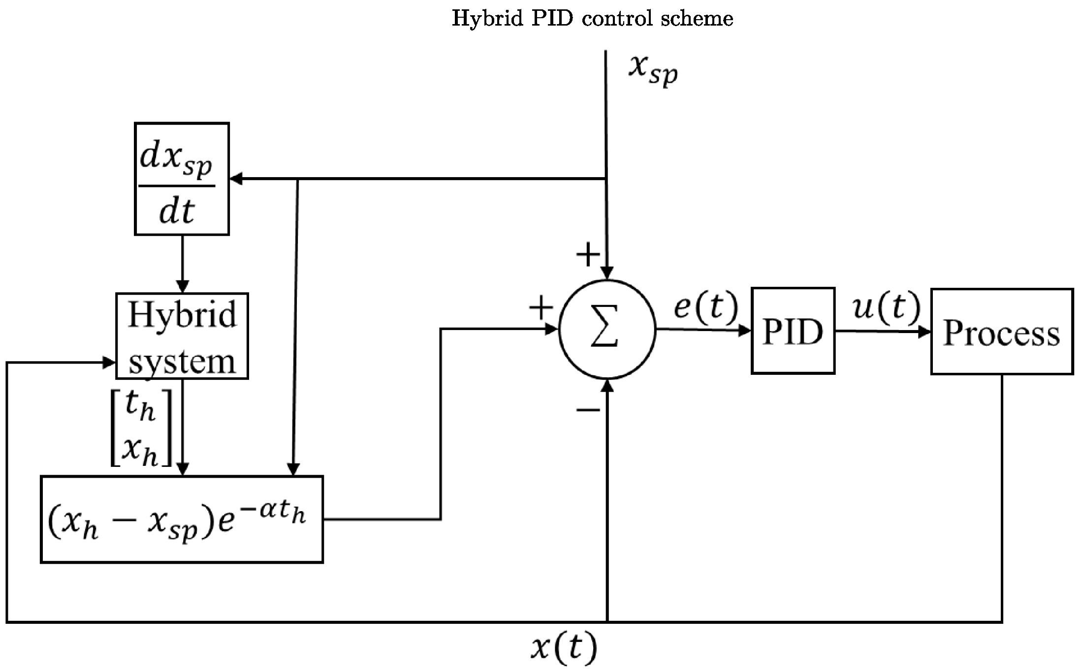
To achieve this, the control scheme shown in Figure 1 is modified as illustrated in Figure 2, where the PID block consists of the components enclosed within the dotted line in Figure 1.

The difference between the control schemes illustrated in Figure 1 and Figure 2 lies in the error signals, $e\left(t\right)$, used by the PID controllers, which differ significantly. In a classical (typical) PID controller scheme, the error is simply defined as the difference between the setpoint and the variable to be regulated. Instead, the proposed approach incorporates an additional exponential component in the error signal, with its parameters determined by a hybrid system. These two features give the PID controller its adaptive behavior. A detailed explanation of this new control algorithm is given below.

2.3.1. The Hybrid System

The proposed control scheme includes a hybrid system whose inputs are the setpoint $x_{sp}$ and its time derivative, namely ${\dot{x}}_{sp}$. Clearly, when the setpoint is a constant value, its derivative is zero. Thus according to (3), this hybrid system is defined as follows:

$$\left[\begin{array}{c}{\dot{t}}_h\hfill \\ {\dot{x}}_h\hfill \end{array}\right]=\left[\begin{array}{c}1\hfill \\ 0\hfill \end{array}\right],$$

(4)

with

$${\left[\begin{array}{c}{t}_h\hfill \\ x_h\hfill \end{array}\right]}^{+}=\left[\begin{array}{c}0\\ x\left(t\right)\end{array}\right],$$

(5)

and the reset condition given by ${\dot{x}}_{sp}\ne 0$. Notice that the state $\left[\begin{array}{c}{t}_h\\ x_h\end{array}\right]$ of the hybrid system (4) and (5) is set to $\left[\begin{array}{c}0\\ x\left(t\right)\end{array}\right]$ each time the reset condition is satisfied, where $x\left(t\right)$ is the value of the variable to be regulated at instant t. As will be clarified below, $t_h$ and $x_h$ are time and the starting point for the exponential function, respectively.

2.3.2. The Exponential Trajectory to the Setpoint

As mentioned before, the proposed control scheme considers an exponential function, which is reset by the state of the hybrid system described earlier. The structure of such and exponential function is

$$\left(x_h-x_{sp}\right)exp(-\alpha t_h).$$

(6)

Here, $-\alpha$ represents the decay rate, where $\alpha$ is the decay factor, which is a positive real number and a design parameter. Additionally, $x_h$ and $t_h$ are values provided by the hybrid system, and $x_{sp}$ denotes the setpoint.

According to Figure 2, the error $e\left(t\right)$ is expressed as follows:

$$e\left(t\right)=x_{sp}+\left(x_h-x_{sp}\right)exp(-\alpha t_h)-x\left(t\right),$$

(7)

but at every instant the hybrid system is reset, i.e., when $t=t_r$, the expression (7) simplifies to

$$\begin{array}{ccc}\hfill e\left(t\right)& =& x_{sp}+\left(x_h-x_{sp}\right)-x\left(t\right),\hfill \\ \hfill e\left(t\right)& =& x_h-x\left(t\right),\hfill \end{array}$$

(8)

because at the reset instant $t=t_r$, $t_h$ is set to zero. Additionally, from (7), it follows that

$$\underset{t_h\to \infty }{lim}e\left(t\right)=x_{sp}-x\left(t\right),$$

(9)

where $t_r$ are the instants at which the hybrid system is reset.

At this point, the following results naturally arise.

Theorem 1.

Suppose the following assumptions hold:

• The value $x\left(t\right)$ is available at all t.
• The design parameter $\alpha \in \mathbb{R}$ satisfies $\alpha >0$ and the envelope generated by $exp(-\alpha t_h)$ is bounded by the system response under the influence of the mistuned PID controller.
• The hybrid system (4)–(5) is reset at instant $t=t_r$.
• There exist gains $K_P$, $K_I$, and $K_D$ (and possibly N) such that the PID controller given by (1) (or correspondingly (2)) is capable of stabilizing the process variable $x\left(t\right)$ in a neighborhood of $x_{sp}$.

Then, the exponential function (6) starts from $x_h=x\left(t\right)$ with $t_h=0$ at $t=t_r$. Furthermore, the exponential function (6) tends asymptotically to zero as $t\to \infty$. Consequently, the error defined by (7) is reset at $t=t_r$ starting at $x_h-x\left(t\right)$ and tending to $x_{sp}-x\left(t\right)$ as $t\to \infty$, and accordingly, the PID controller (1) (or correspondingly (2)) takes the process variable $x\left(t\right)$ to a neighborhood of $x_{sp}$ following an exponential trajectory.

Proof. 

The proof follows directly from the previous discussion. □

Remark 1.

“Exponential trajectory to the setpoint”: Notice that at the instants when the hybrid system is reset, namely when $t=t_r$, the error $e\left(t\right)$ is initially zero rather than $x_{sp}-x\left(t\right)$. This characteristic often leads to a significant reduction in the magnitude of the PID controller’s output. The reason for this behavior lies in the exponential function, which is reset at $t=t_r$ to start from the current value of $x\left(t\right)$, i.e., $x_h=x\left(t\right)$ and $t_h=0$. Subsequently, the exponential function (6) asymptotically approaches zero as $t_h\to \infty$. As a result, the error $e\left(t\right)$ gradually converges to $e\left(t\right)=x_{sp}-x\left(t\right)$, leading to a smooth and progressive reduction in $e\left(t\right)$.

Remark 2.

Note that the selection of the decay rate α depends on the behavior induced by the mistuned PID in the sense that α should be selected to produce a slower behavior than that induced by the classical PID, thus maintaining the stability originally provided by the PID controller. Furthermore, the exponential function, which is restored by the hybrid system, ensures that the error remains bounded. In other words, the envelope generated by $exp(-\alpha t_h)$ must be bounded by the system response under the influence of the mistuned PID controller.

Remark 3.

The proposed hybrid PID controller performs the same core operations as the conventional PID controller but introduces an additional step: the evaluation of an exponential reference trajectory at each time instant. This step involves a single exponential function computation and a simple reset condition, typically implemented using a modulo operation and a few multiplications. The added computational cost is minimal and easily manageable in modern control hardware.

3. Simulation and Experimental Validation

3.1. Numerical Validation on a Robotic System

To validate the previous results, the robotic arm analyzed in [23] and depicted in Figure 3 is considered.

The dynamics of this system is given by the following:

$$u\left(t\right)=D\left(\theta \left(t\right)\right)\ddot{\theta }\left(t\right)+h(\theta \left(t\right),\dot{\theta }\left(t\right))+C\left(\theta \right)$$

(10)

where

$$D\left(\theta \left(t\right)\right)=\left[\begin{array}{cc}{d}_{11}\left(\theta \left(t\right)\right)& d_{12}\left(\theta \left(t\right)\right)\\ d_{21}\left(\theta \left(t\right)\right)& d_{22}\left(\theta \left(t\right)\right)\end{array}\right],$$

(11)

$$h(\theta \left(t\right),\dot{\theta }\left(t\right))=\left[\begin{array}{c}{h}_1(\theta \left(t\right),\dot{\theta }\left(t\right))\\ h_2(\theta \left(t\right),\dot{\theta }\left(t\right))\end{array}\right],$$

(12)

$$c\left(\theta \left(t\right)\right)=\left[\begin{array}{c}{c}_1\left(\theta \left(t\right)\right)\\ c_2\left(\theta \left(t\right)\right)\end{array}\right],u\left(t\right)=\left[\begin{array}{c}{u}_1\left(t\right)\\ u_2\left(t\right)\end{array}\right],$$

(13)

and $d_{11}\left(\theta \left(t\right)\right)={\displaystyle \frac{1}{3}}{m}_1{l}^2+{\displaystyle \frac{4}{3}}{m}_2{l}^2+m_{2}cos\left({\theta }_2\left(t\right)\right)l^2$, $d_{12}\left(\theta \left(t\right)\right)={\displaystyle \frac{1}{3}}{m}_2{l}^2+{\displaystyle \frac{1}{2}}{m}_2{l}^{2}cos\left({\theta }_2\left(t\right)\right)$, $d_{21}\left(\theta \left(t\right)\right)={\displaystyle \frac{1}{3}}{m}_2{l}^2+{\displaystyle \frac{1}{2}}{m}_2{l}^{2}cos\left({\theta }_2\left(t\right)\right)$, $d_{22}\left(\theta \left(t\right)\right)={\displaystyle \frac{1}{3}}{m}_2{l}^2$, $c_1\left(\theta \left(t\right)\right)={\displaystyle \frac{1}{2}}{m}_{1}glcos\left({\theta }_1\left(t\right)\right)+{\displaystyle \frac{1}{2}}{m}_{2}glcos({\theta }_1\left(t\right)+{\theta }_2\left(t\right))+m_{2}glcos\left({\theta }_1\left(t\right)\right)$, $c_2\left(\theta \left(t\right)\right)={\displaystyle \frac{1}{2}}{m}_{2}glcos({\theta }_1\left(t\right)+{\theta }_2\left(t\right))$, $h_1(\theta \left(t\right),$$\dot{\theta }\left(t\right))={\displaystyle \frac{1}{2}}{m}_{2}sin\left({\theta }_2\left(t\right)\right)l^2{\dot{\theta }}_2^2-m_{2}sin\left({\theta }_2\left(t\right)\right)l^2{\dot{\theta }}_1\left(t\right){\dot{\theta }}_2$, $h_2(\theta \left(t\right),\dot{\theta }\left(t\right))={\displaystyle \frac{1}{2}}{m}_{2}sin\left({\theta }_2\left(t\right)\right)l^2{\dot{\theta }}_1{\left(t\right)}^2$. where ${\theta }_1\left(t\right)$ is the angle (in radians) between the inner link and the horizontal axis, ${\theta }_2\left(t\right)$ represents the angle (in radians) between the outer link and the inner link, $x_2\left(t\right)={\dot{\theta }}_1$ is the angular velocity of the inner link and $x_4\left(t\right)={\dot{\theta }}_2$ is the angular velocity of the outer link.

The rigid links have masses of $m_1=0.4\mathrm{kg}$ and $m_2=0.3\mathrm{kg}$, while lengths $l=l_1=l_2=0.5\mathrm{m}$. The input torques applied to the system are denoted as $u_1\left(t\right)$ and $u_2\left(t\right)$, both measured in $N·m$. The gravitational acceleration is $g=9.81{\mathrm{m}/\mathrm{s}}^2$.

Also consider that the control signals $u_1\left(t\right)$ and $u_2\left(t\right)$ are generated by two mistuned PID controllers of the form (2), with parameters $K_P=100$, $K_I=10$, $K_D=5$, and $N=300$ for both PIDs.

In the following examples, the robotic arm starts at rest from the lower vertical position, with initial conditions ${\theta }_1\left(0\right)={\displaystyle \frac{3\pi }{2}}$, ${\dot{\theta }}_1\left(0\right)=0$, ${\theta }_2\left(0\right)=0$, and ${\dot{\theta }}_2\left(0\right)=0$. Then, both the typical PID controller and the proposed controller are applied to move the robotic arm to different setpoints during $15\mathrm{s}$, illustrating the distinct behaviors induced by these controllers.

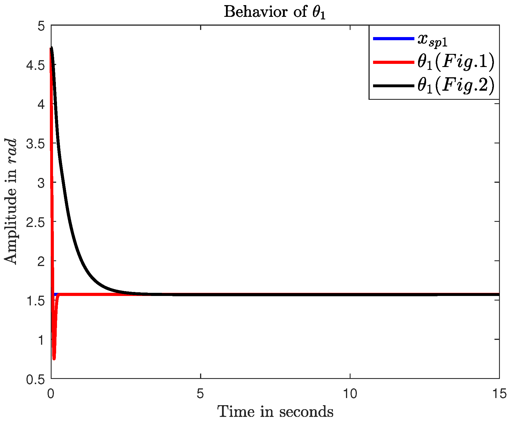
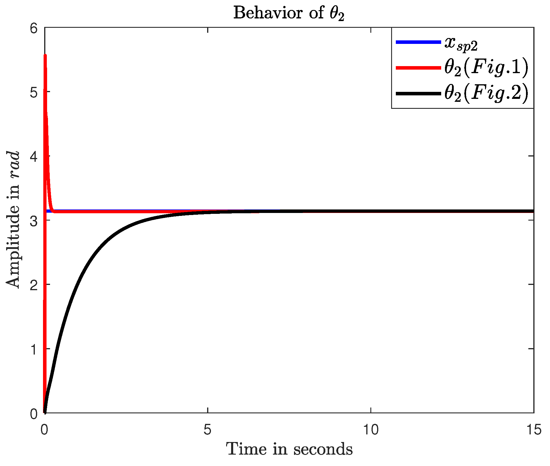
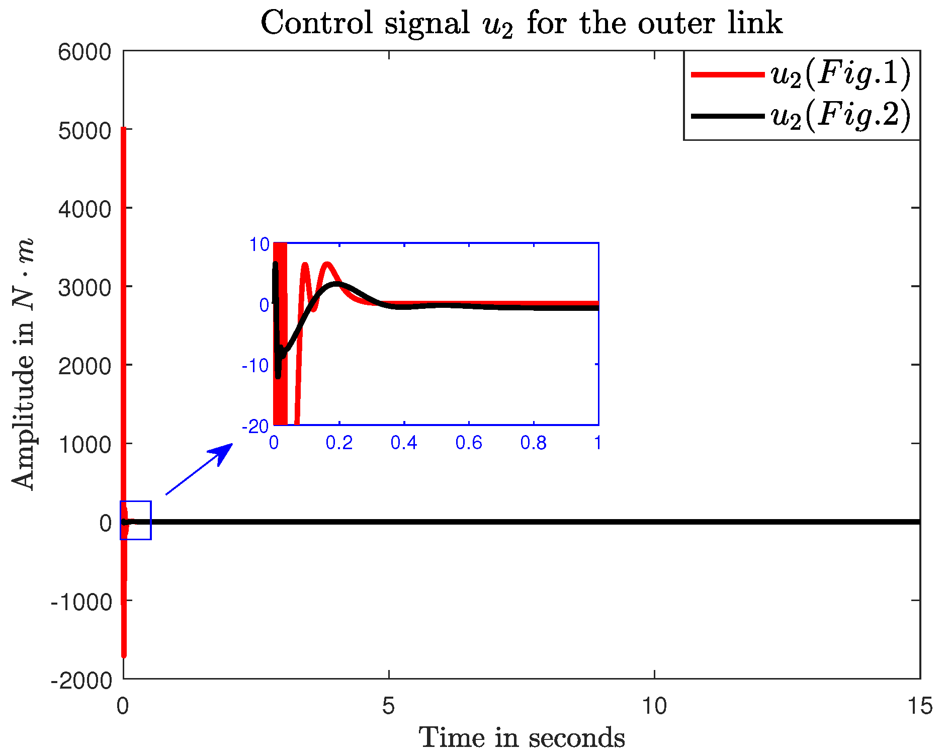
3.1.1. Example 1: Constant Setpoint

In this numerical experiment, the control goal is to move the robotic arm from its initial conditions to ${\theta }_1=x_{sp1}$ and ${\theta }_2=x_{sp1}$, where $x_{sp1}={\displaystyle \frac{\pi }{2}}$ and $x_{sp2}=\pi$ are the respective setpoints. First, the control scheme depicted in Figure 1 is applied. Then, the proposed control scheme shown in Figure 2 is applied, assuming that the reset parameter $\beta$ for each of the two hybrid systems can be neglected because both setpoints are constant. On the other hand, the decay rate parameters of the exponential functions in expression (6) are set to ${\alpha }_1=2$ and ${\alpha }_2=1$ for the inner and outer controllers, respectively. The results are presented in Figure 4, Figure 5, Figure 6 and Figure 7. Evidently, the proposed control scheme shown in Figure 2 allows for a smoother behavior of the link, with significantly reduced control signal amplitudes, even when using the same PID gains. Also note how the inner link converges faster than the outer link to the setpoint due to the decay rates chosen for the corresponding exponential functions. However, if the decay rates are assigned the same values, both links will converge to their respective setpoints at the same rate.

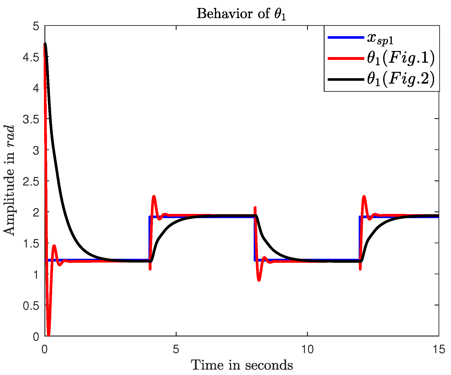
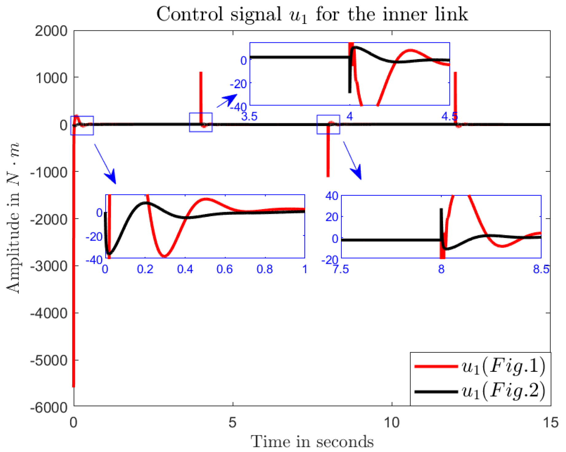
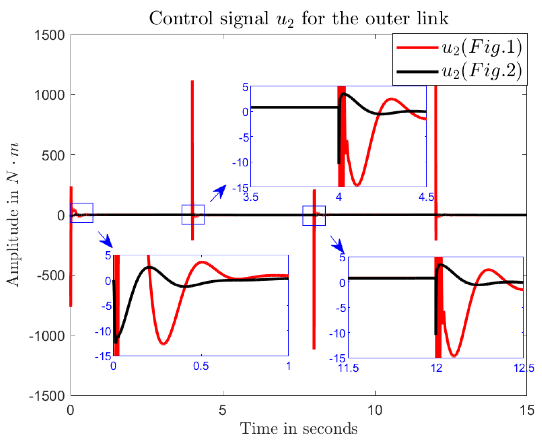
Remark 4.

Although the behavior achieved by the proposed control scheme can approximate that of the classical scheme shown in Figure 1, the classical scheme requires much more precise tuning of the PID controllers.

3.1.2. Example 2: Discontinuously Changing Setpoint

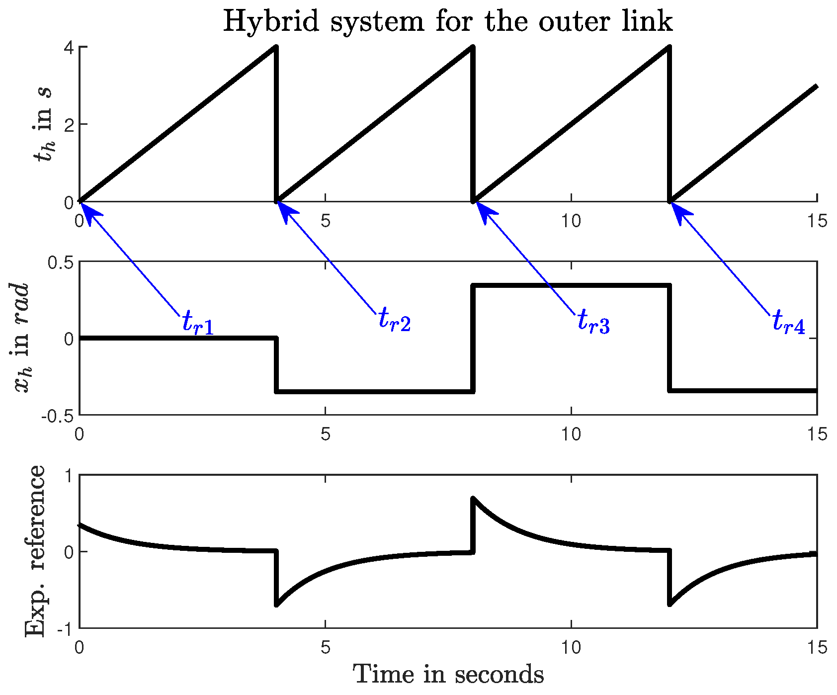
In this example, the setpoints for each of the links are defined as step functions with an amplitude of ${\displaystyle \frac{\pi }{9}}rad$ and a frequency of ${\displaystyle \frac{\pi }{4}}{\displaystyle \frac{rad}{s}}$. Thus, $t_{r1}=0$, $t_{r2}=4\mathrm{s}$, $t_{r3}=8\mathrm{s}$, and $t_{r4}=12\mathrm{s}$. For the reset conditions of the hybrid systems, as mentioned above, it is sufficient to set them as $\parallel {\dot{x}}_{sp1}\parallel \ne 0$ and $\parallel {\dot{x}}_{sp2}\parallel \ne 0$ since the setpoints change in a discontinuous way. The PID gains and the decay rates for the exponential functions are the same as those used in the previous example.

With this in mind, as before, the classical scheme shown in Figure 1 and the proposed scheme depicted in Figure 2 are applied, with the results presented in Figure 8, Figure 9, Figure 10, Figure 11, Figure 12 and Figure 13.

Again, based on the hybrid system and the exponential functions considered, the proposed control scheme provides smooth trajectories to the setpoints and reduces the amplitudes of the control signals.

3.2. Experimental Validation on an Aeronautical System: Hybrid PID Control for Quadcopter Takeoff and Landing

Commercial quadcopters typically use separate control sequences for takeoff and landing, requiring the user or an automated system to select the appropriate sequence for proper execution. To overcome this limitation, the proposed hybrid PID control scheme was applied to manage both takeoff and landing using the default gains of the quadcopter’s hover PID controller. Specifically, the PID controllers that regulate lateral, longitudinal, and angular displacements remained unchanged.

Although the mathematical model of a quadcopter (or quadrotor), such as the one shown in Figure 14, is discussed in detail in [24,25], this section focuses on directly applying the proposed approach to the quadrotor depicted in Figure 15 using the Simulink Support Package for Parrot Minidrones. This MATLAB toolbox allows users to connect to the quadrotor via Bluetooth, providing access to its sensors and actuators. This package includes a controller project template designed as a framework for developing a custom controller or adapting it to specific requirements. The template integrates a comprehensive simulation of the plant model for the Parrot Rolling Spider and Parrot Mambo drones, allowing users to evaluate the performance of the model prior to deployment. This enables a thorough analysis and refinement of controller designs prior to implementation on physical hardware. Additionally, the template supports six-degree-of-freedom (6-DOF) motion equation modeling, enabling the simulation of aircraft behavior under various flight and environmental conditions. 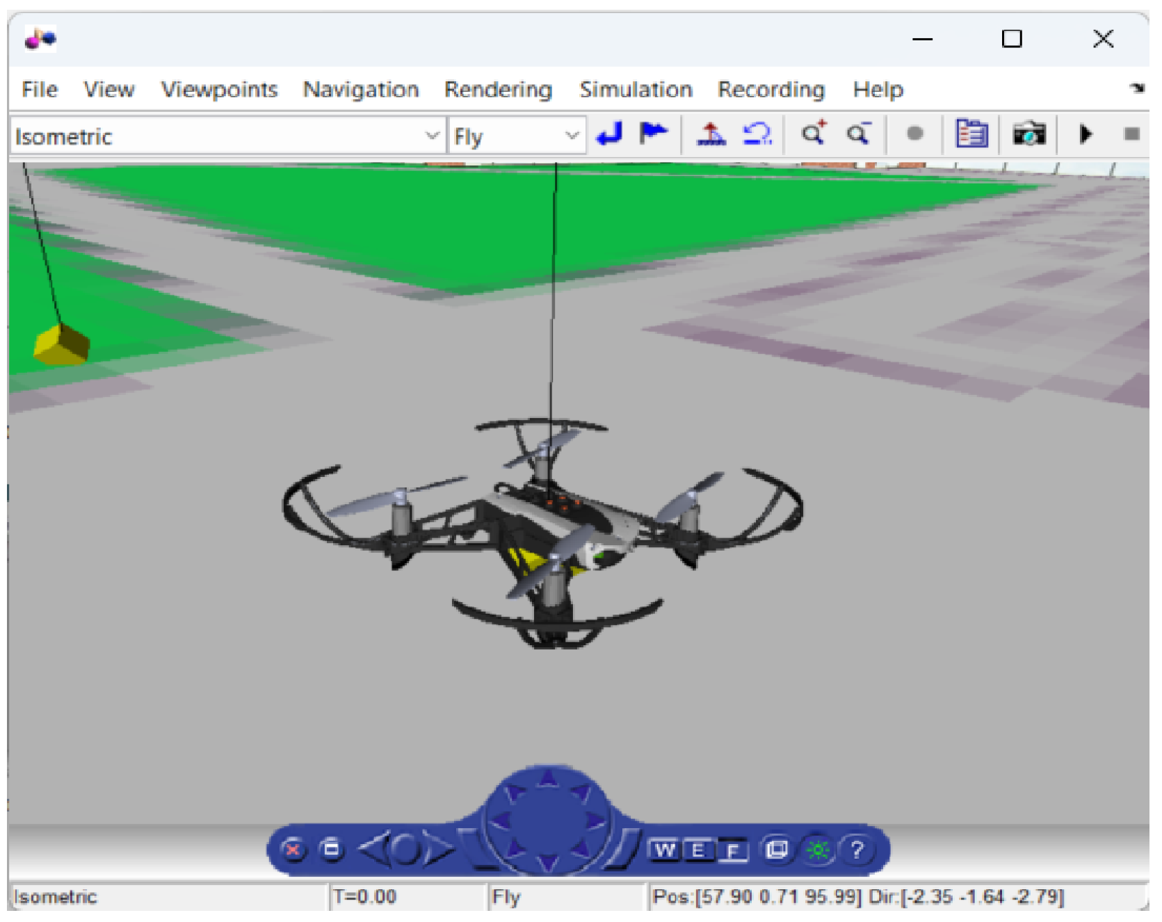Figure 15 illustrates the Virtual Reality Modeling Language (VRML) environment used by the Simulink package for Parrot Minidrones [26,27].

Remark 5.

The Simulink support package for Parrot Minidrones has undergone extensive validation, demonstrating high accuracy in approximating the real-time behavior of these drones.

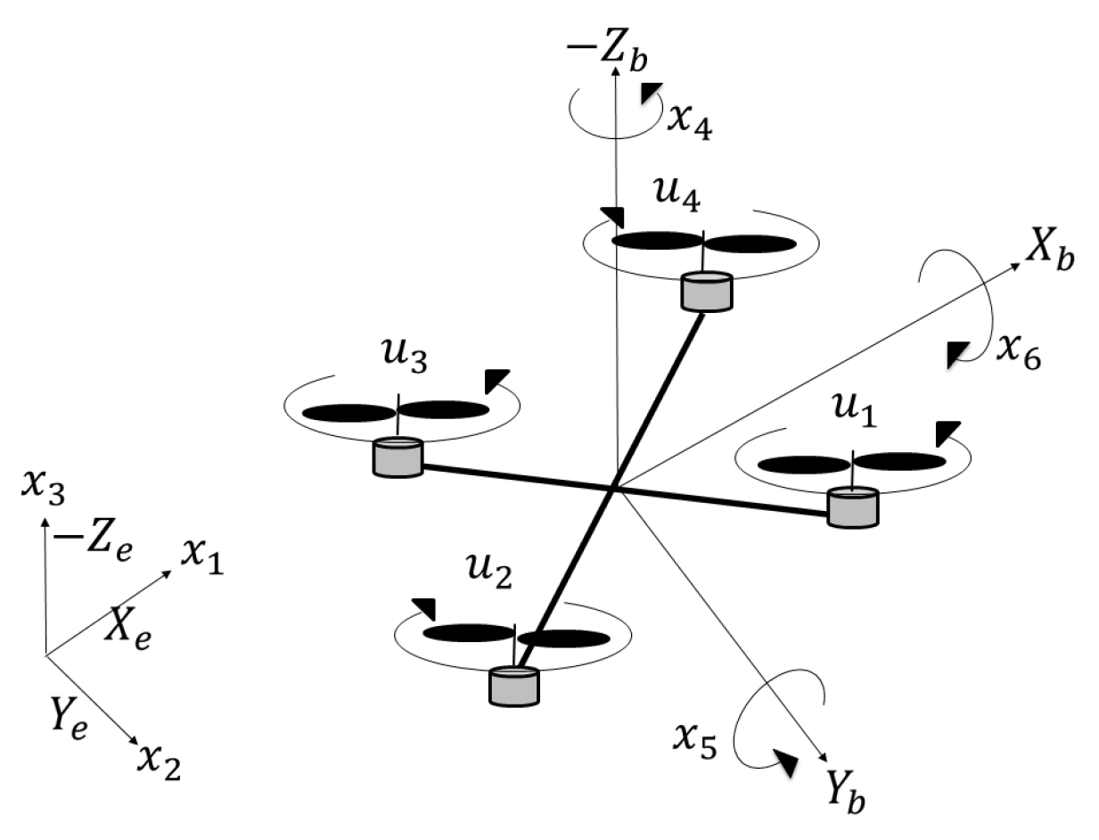
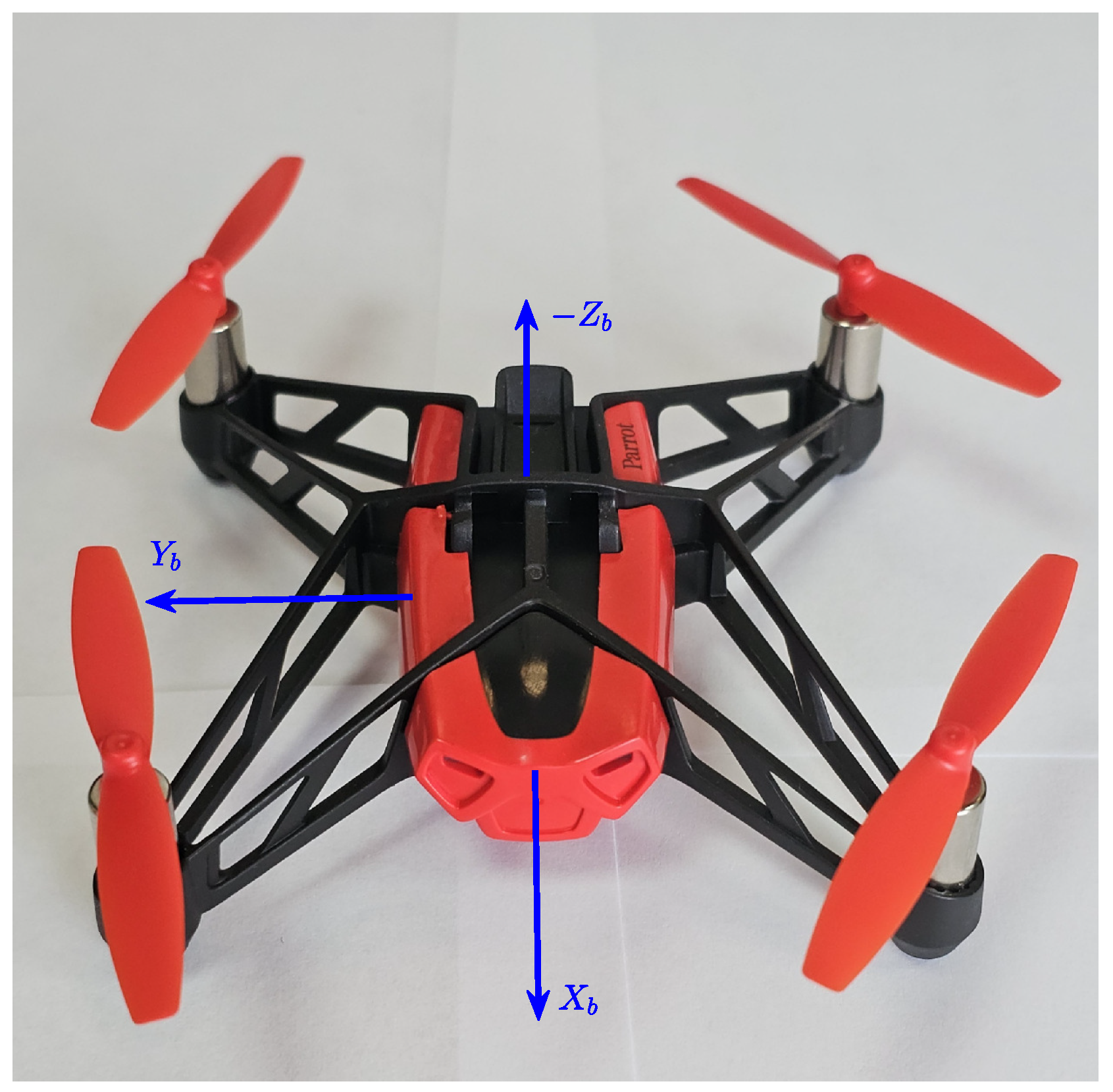
Remark 6.

According to the right-hand rule, which is the standard convention in aeronautics, the altitude axis $Z_b$ is defined as negative in the upward direction. This ensures consistency with the body-fixed coordinate system, where the $X_b$-axis points forward and the $Y_b$-axis points to the right of the drone [25].

As in the previous examples, the analytical design of the thrust PID controller is omitted. Instead, the default gains provided by the MATLAB’s toolbox, together with the control scheme discussed above, are used to achieve take-off and landing of the Parrot Rolling Spider depicted in Figure 16. It is important to mention that the default thrust PID controller has the form of (2) but works in discrete time, with the following gains: $K_P=0.8$, $K_I=0$, $K_D=0.3$, and $N=50$. In practice, this results in a PD controller.

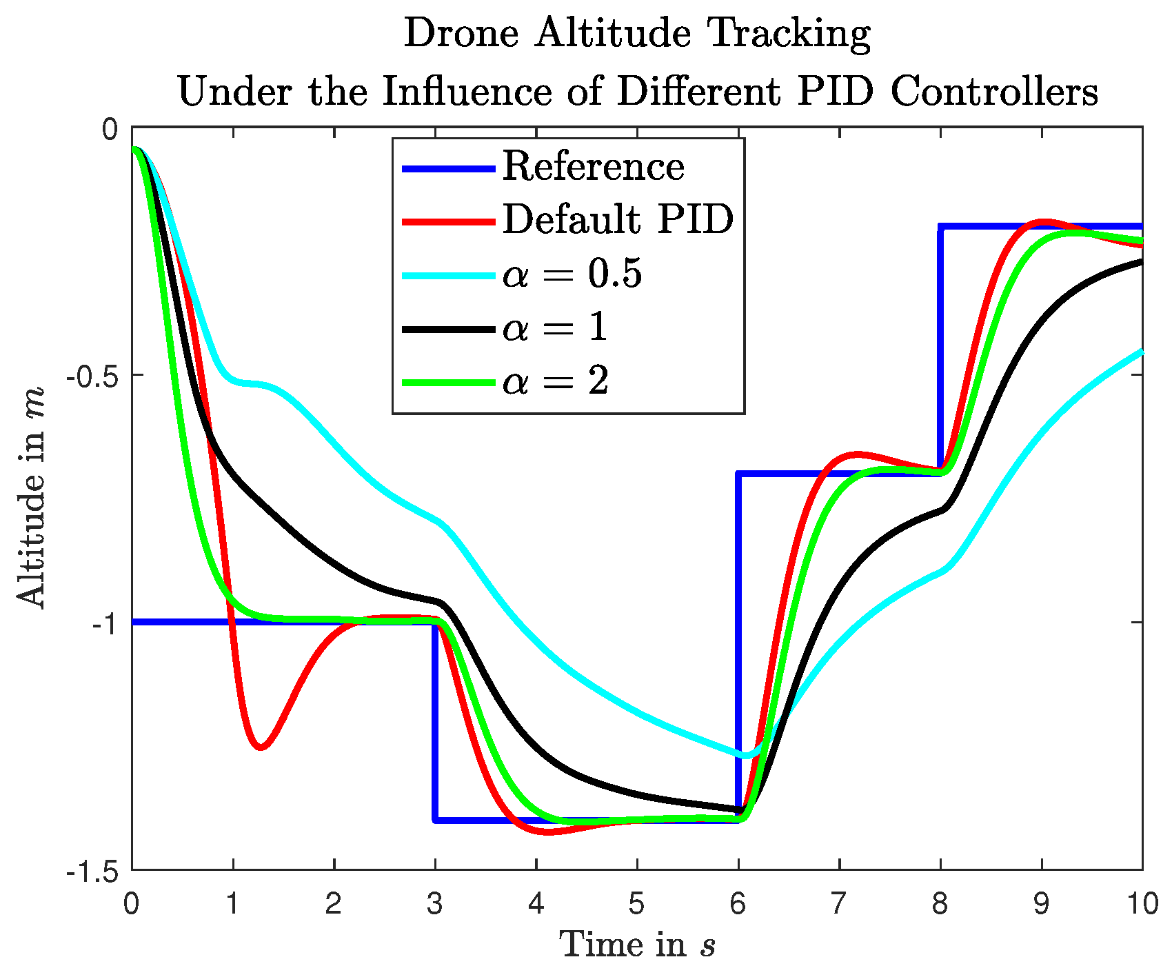
Before implementing the hybrid PID controller on the Parrot Rolling Spider in real-time, simulations were conducted using the MATLAB toolbox. In these simulations, the drone was required to take off and stabilize at an altitude of $x_{sp1}=1\mathrm{m}$. Then, at $t=3\mathrm{s}$, the setpoint was increased to $x_{sp2}=1.4\mathrm{m}$. At $t=6\mathrm{s}$, the setpoint was decreased to $x_{sp3}=0.7\mathrm{m}$, followed by a final setpoint change to $x_{sp4}=0.2\mathrm{m}$ at $t=8\mathrm{s}$. The landing was completed by turning off the motors at $t=10\mathrm{s}$.

The four cases considered were the (1) original PID, (2) hybrid PID with $\alpha =0.5$, (3) hybrid PID with $\alpha =1$, and (4) hybrid PID with $\alpha =2$. The results are presented in Figure 17, Figure 18, Figure 19, Figure 20, Figure 21 and Figure 22.

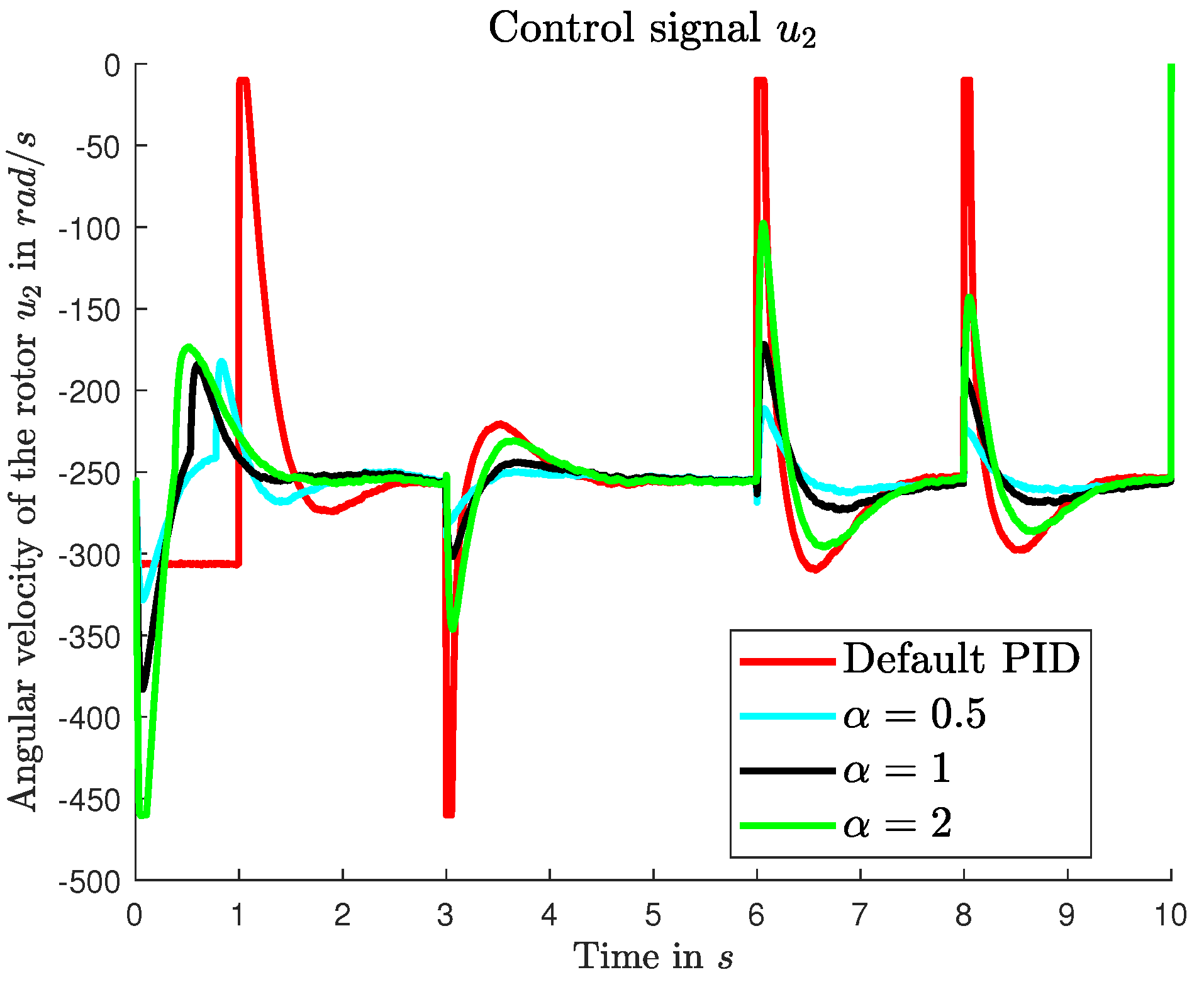
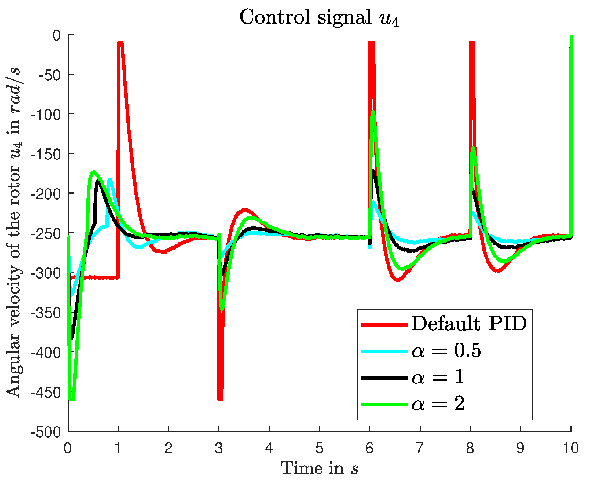
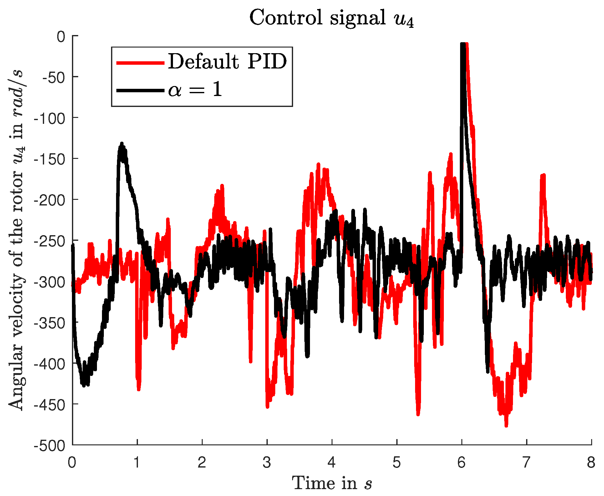
Remark 7.

As expected, from Figure 15, Figure 16, Figure 17, Figure 18, Figure 19, Figure 20, Figure 21 and Figure 22, it can be observed that the drone reaches the setpoints more smoothly when the hybrid controller is used, requiring less effort from the actuators and consequently saving energy. Furthermore, it is evident that smaller values of α result in a slower response towards the setpoint. It is important to note that the PID gains remain the same for all cases, as mentioned above.

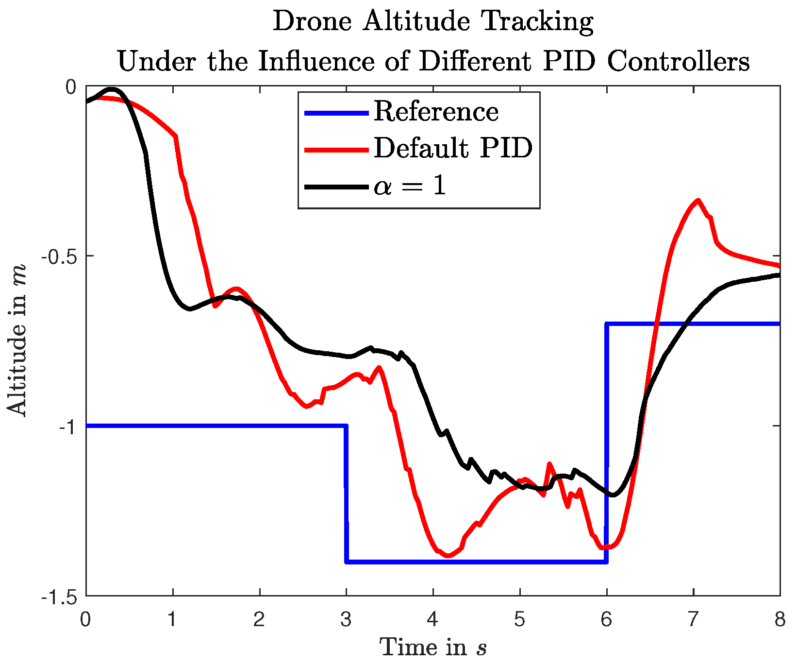
The same flight scheme was applied to the Parrot Rolling Spider in real-time with two control schemes: (1) the default PID provided by the MATLAB toolbox and (2) the hybrid PID controller with $\alpha =1$. The real-time flight data are presented in Figure 23, Figure 24, Figure 25, Figure 26 and Figure 27.

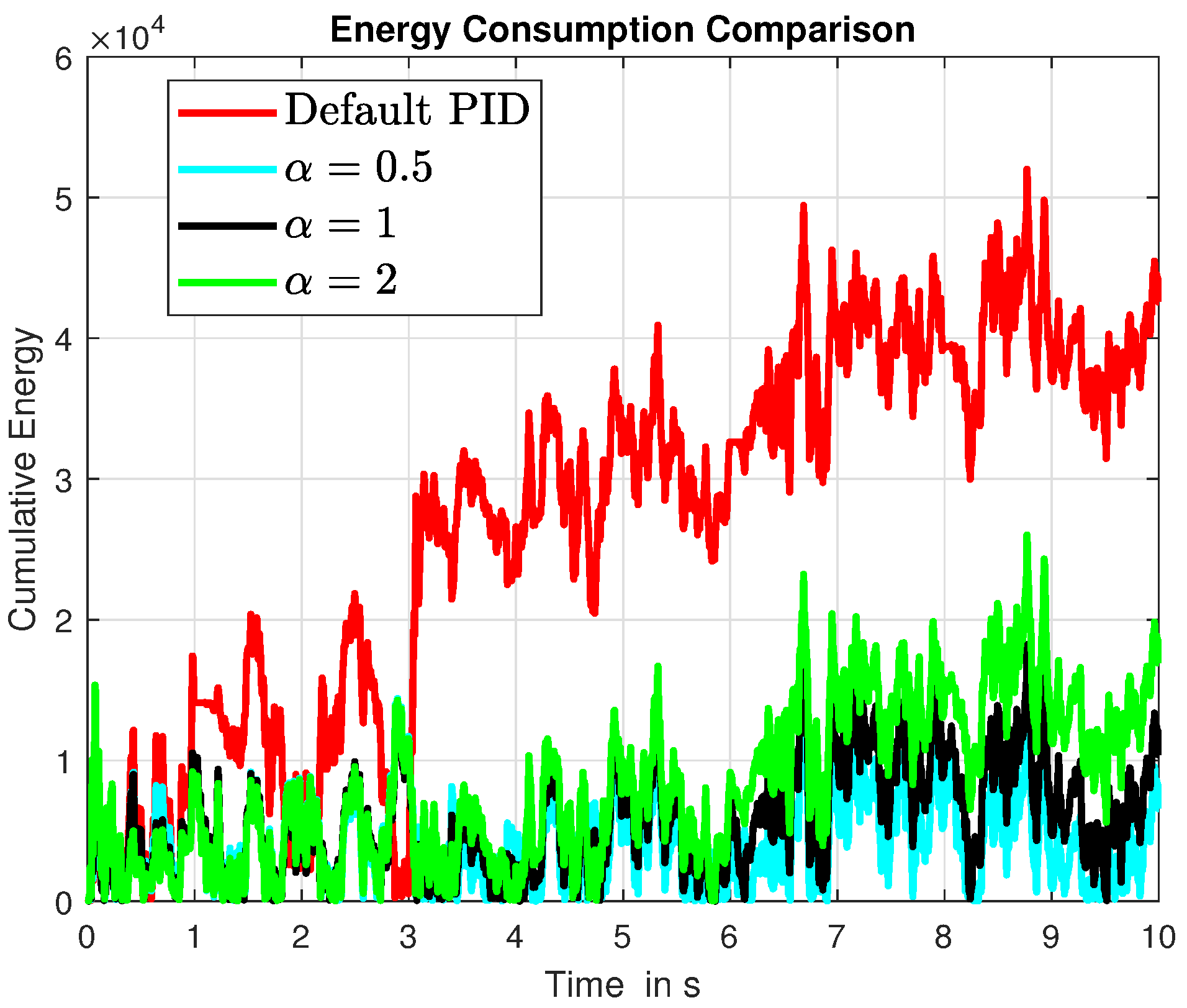
3.3. Energy Efficiency of Control Strategies

In this brief section, a comparative analysis of the classical PID controller and the hybrid PID controllers with decay rates $\alpha =0.5$, $\alpha =1$, and $\alpha =2$ is presented, with a focus on energy consumption. The analysis is based on numerical simulations conducted on the quadrotor model described in the previous section. To this end, the rotor power expression considered is as follows:

$$P_i=k_p·u_i^3,$$

(14)

where $u_i$ represents the angular velocity of rotor i in radians per second, and $k_p$ is a power coefficient that depends on rotor characteristics and air density. For simplicity, $k_p$ is assumed to be equal to 1 in this study.

The relative energy savings achieved by the hybrid approaches, in comparison to the classical PID, are summarized in

Table 1. Relative energy savings of the hybrid PID controller for different values of $\alpha$.

Decay Rate $\mathit{\alpha }$	Relative Energy Savings (%)
0.5	84.55
1.0	75.56
2.0	60.26

. Additionally, a graphical comparison of the cumulative energy consumption is provided in Figure 28.

As expected, the hybrid controller with $\alpha =0.5$ exhibits the highest energy efficiency as its slower dynamics reduce the effort on the rotors more effectively compared to higher values of $\alpha$. It is important to note that these results may vary depending on the quality of the tuning of the classical PID controller.

4. Discussion

As observed in the simulation results, the drone operating in real time with the proposed hybrid PID controller exhibits significantly smoother dynamic behavior compared to the classical PID scheme. This improvement is evident in the reduction in oscillations and overshoot during transient responses, leading to enhanced stability and tracking performance. Notably, the hybrid controller achieves this improvement without altering the PID gains as both the classical and hybrid controllers operate with the same parameter settings.

Furthermore, a noticeable reduction in actuator effort is achieved when employing the hybrid PID controller. This reduction suggests more efficient control actions, which translate into lower energy consumption—an essential factor in battery-operated aerial vehicles such as drones. The decrease in control signal intensity, without compromising performance, highlights the effectiveness of the hybrid approach in optimizing resource utilization.

These results demonstrate that the proposed hybrid PID controller not only meets the desired control objectives but also offers tangible benefits in terms of energy efficiency. Consequently, it can be concluded that, even in real-time implementations, the hybrid control strategy is a viable and advantageous alternative to the classical PID approach, particularly in applications where energy conservation and smooth operation are critical.

5. Conclusions

This paper presented a control scheme that integrates hybrid systems, exponential functions, and a PID controller to achieve smooth trajectory transitions of the process variable to the setpoint. The hybrid system enables dynamic resetting of the exponential function parameters, ensuring that even in the presence of discontinuous setpoint changes, the process variable smoothly converges to the new target.

Through both numerical simulations and real-time experiments, it was demonstrated that the proposed approach effectively reduces transient oscillations typically caused by poorly tuned PID controllers. This results in reduced actuator effort and, consequently, energy savings. Notably, the same PID gain values were used for both the classical and hybrid PID controllers, highlighting the improved performance of the proposed method without additional tuning requirements.

It is important to highlight a potential limitation of the proposed hybrid control strategy. Specifically, the method’s performance may be compromised if the decay rate $\alpha$ is selected too aggressively, that is, when the resulting exponential trajectory demands a faster closed-loop response than the original PID controller can stably achieve. In such cases, the hybrid mechanism may impose excessive control effort or even destabilize the system. Therefore, to preserve the stability guaranteed by the original PID controller, it is suggested to select $\alpha$ such that the exponential reference evolves more slowly than the system under the influence of the original PID. This consideration is crucial for practical implementation and underscores the need for careful parameter selection, as explained in more detail in Remarks 2 and 3.

As future work, it is proposed to explore alternative functions to replace the exponential function, providing different trajectory shaping strategies for setpoint tracking. Additionally, extending the approach to other control applications and refining the hybrid switching mechanism could further enhance its adaptability and effectiveness.

References

- Åström, K.J.; Hägglund, T. PID Controllers: Theory, Design, and Tuning, 2nd ed.; Instrument Society of America: Pittsburgh, PA, USA, 1995; Available online: https://aiecp.files.wordpress.com/2012/07/1-0-1-k-j-astrom-pid-controllers-theory-design-and-tuning-2ed.pdf (accessed on 16 December 2024).
- Ziegler, J.G.; Nichols, N.B. Optimum settings for automatic controllers. Trans. ASME 1942, 64, 759–768. [Google Scholar] [CrossRef]
- Ang, K.H.; Chong, G.C.Y.; Li, Y. PID Control System Analysis, Design, and Technology. IEEE Trans. Control Syst. Technol. 1942, 13, 559–576. [Google Scholar] [CrossRef]
- Moin, H.; Shah, U.H.; Khan, M.J.; Sajid, H. Fine-Tuning Quadcopter Control Parameters via Deep Actor-Critic Learning Framework: An Exploration of Nonlinear Stability Analysis and Intelligent Gain Tuning. IEEE Access 2024, 12, 173462–173474. [Google Scholar] [CrossRef]
- Liberzon, D. Switching in Systems and Control; Birkhäuser: Boston, MA, USA, 2003; Available online: https://link.springer.com/book/10.1007/978-1-4612-0017-8 (accessed on 16 December 2024).
- Kelly, R.; Santibáñez, V.; Loría, A. Control of Robot Manipulators in Joint Space; Springer: London, UK, 2005; Available online: https://link.springer.com/book/10.1007/b135572 (accessed on 16 December 2024).
- Yang, Q.; Chen, G.; Guo, M.; Chen, T.; Luo, L.; Sun, L. Model Predictive Hybrid PID Control and Energy-Saving Performance Analysis of Supercritical Unit. Energies 2024, 17, 6356. [Google Scholar] [CrossRef]
- Mohamed Iqbal, M.; Pavithra, C.V.; Nithiyananthan, K.; Yousuff, M. Fuzzy gain Scheduled PID Controller for Power Quality Enhancement in Grid Connected Hybrid Solar PV-PEMFC Energy System. J. Eng. Res. 2023, 11, 146–156. [Google Scholar] [CrossRef]
- Mehbodniya, A.; Kumar, P.; Xie, C.; Webber, J.L.; Mamodiya, U.; Halifa, A.; Srinivasulu, C. Hybrid Optimization Approach for Energy Control in Electric Vehicle Controller for Regulation of Three-Phase Induction Motors. Math. Probl. Eng. 2022, 2022, 6096983. [Google Scholar] [CrossRef]
- Hosseini, R.; Kumar, P.; Mashayekhi Fard, J.; Soltani, S. Active filter design and synthesis for hybrid neuro-fuzzy and robust PID controllers. Int. J. Dyn. Control 2024, 12, 3873–3883. [Google Scholar] [CrossRef]
- Yang, Q.; Zhang, F.; Wang, C. Deterministic Learning-Based Neural PID Control for Nonlinear Robotic Systems. IEEE/CAA J. Autom. Sin. 2024, 11, 1227–1238. [Google Scholar] [CrossRef]
- Jasim Mohamed, M.; Oleiwi, B.K.; Azar, A.T.; Mahlous, A.R. Hybrid controller with neural network PID/FOPID operations for two-link rigid robot manipulator based on the zebra optimization algorithm. Front. Robot. AI 2024, 11, 386968. [Google Scholar] [CrossRef] [PubMed]
- Meseret, G.M.; Saikia, L.C. Hybrid neuro-fuzzy-based 3DOF-PDN controller for AGC of multi-area interconnected power system incorporated hydrogen aqua electrolyze fuel cell units and unified power flow controller. Electr. Eng. 2024, 1–19. [Google Scholar] [CrossRef]
- Demirtaş, M. A Hybrid Algorithm for Adaptive Neuro-controllers. Black Sea J. Eng. Sci. 2023, 6, 87–97. [Google Scholar] [CrossRef]
- Celik, O.M.; Deniz, F.N.; Koseoglu, M. Design of Hybrid MPC-PID Controller Based on Fractional Order Model of AMR. IEEE Access 2025, 13, 89556–89569. [Google Scholar] [CrossRef]
- Nazir, K.; Kim, Y.-W.; Byun, Y.-C. Predictive PID Control for Automated Guided Vehicles Using Genetic Algorithm and Machine Learning. IEEE Access 2025, 13, 66726–66741. [Google Scholar] [CrossRef]
- Kumar, T.R.D.; Mija, S.J. Boundary Logic-Based Hybrid PID-SMC Scheme for a Class of Underactuated Nonlinear Systems-Design and Real-Time Testing. IEEE Trans. Ind. Electron. 2025, 72, 5257–5267. [Google Scholar] [CrossRef]
- Yao, Z.; Liang, X.; Wang, S.; Yao, J. Model-Data Hybrid Driven Control of Hydraulic Euler–Lagrange Systems. IEEE/ASME Trans. Mechatron. 2025, 30, 131–143. [Google Scholar] [CrossRef]
- Bhookya, J. A New Hybrid MFO-WO Algorithm and Its Application to Design of FOPID/PID Controller for IoT Applications. IEEE Access 2025, 13, 14557–14571. [Google Scholar] [CrossRef]
- Beerens, R.; Bisoffi, A.; Zaccarian, L.; Nijmeijer, H.; Heemels, M.; van de Wouw, N. Reset PID Design for Motion Systems With Stribeck Friction. IEEE Trans. Control Syst. Technol. 2022, 30, 294–310. [Google Scholar] [CrossRef]
- Control System Toolbox™ User’s Guide; The MathWorks, Inc. Available online: https://www.mathworks.com/help/pdf_doc/control/index.html (accessed on 12 December 2024).
- Goebel, R.; Sanfelice, R.G.; Teel, A.R. Hybrid Dynamical Systems: Modeling, Stability, and Robustness; JSTOR; Princeton University Press: Princeton, NJ, USA, 2012; Available online: http://www.jstor.org/stable/j.ctt7s02z (accessed on 12 December 2024).
- Meda-Campaña, J.A.; Ancona-Bravo, R.I.; Escobedo-Alva, J.O.; Hernández-Cortés, T.; Tapia-Herrera, R. The Output Regulation Problem for Unmodeled Reference/Disturbance Signals Using High-gain Observers. Int. J. Control Autom. Syst. 2023, 21, 1049–1061. [Google Scholar] [CrossRef]
- Meda-Campaña, J.A.; Torres-Cruz, R.E.; Rojas-Ruiz, A.J.; Tapia-Herrera, R.; Hernández-Cortés, T.; Páramo-Carranza, L.A. The Output Regulation and the Kalman Filter as the Signal Generator. IEEE Access 2023, 11, 90825–90838. [Google Scholar] [CrossRef]
- Velázquez-Sánchez, R.D.; Escobedo-Alva, J.O.; Peña-García, R.; Tapia-Herrera, R.; Meda-Campaña, J.A. Identification of High-Order Nonlinear Coupled Systems Using a Data-Driven Approach. Appl. Sci. 2024, 14, 3864. [Google Scholar] [CrossRef]
- MathWorks. Parrot Minidrones Support from Simulink. 2023. Available online: https://www.mathworks.com/hardware-support/parrot-minidrones.html (accessed on 12 December 2024).
- MathWorks. Simulink Support Package for Parrot Minidrones Documentation. 2023. Available online: https://www.mathworks.com/help/supportpkg/parrot/ (accessed on 12 December 2024).
Figure 1.
Closed-loop system with a classical PID controller scheme.
Figure 2.
Scheme of the closed-loop system with the hybrid PID controller and exponential trajectories for a smooth transition to the setpoint.
Figure 3.
Schematic representation of the robotic arm modeled in MATLAB/Simulink using the Multibody toolbox.
Figure 4.
Behavior of the inner link: red indicates the control scheme shown in
Figure 1, and black represents the control scheme shown in
Figure 5.
Control signal of the inner link: red indicates the control scheme shown in
Figure 6.
Behavior of the outer link: red indicates the control scheme shown in
Figure 7.
Control signal of the outer link: red indicates the control scheme shown in
Figure 8.
Figure 9.
Figure 10.
Figure 11.
Figure 12.
Behavior of the hybrid system included in the hybrid PID scheme for the inner link.
Figure 13.
Behavior of the hybrid system included in the hybrid PID scheme for the outer link.
Figure 14.
Schematic of a generic quadcopter [
25].
Figure 15.
Preview of the VRML environment in the Simulink Support Package for Parrot Minidrones [
Figure 16.
Parrot Rolling Spider.
Figure 17.
Altitude response of the drone compared to the reference trajectory in different PID control strategies.
Figure 18.
Behavior of the rotor input under the influence of different PID controllers.
Figure 19.
Figure 20.
Figure 21.
Figure 22.
States of the hybrid system and the exponential reference.
Figure 23.
Figure 24.
Figure 25.
Figure 26.
Figure 27.
Figure 28.
Cumulative energy consumption for classical PID and hybrid PID controllers with , , and , based on numerical simulation results.