Abstract
Medium- and large-scale heat sinks are critical for thermal load management in high-performance systems. However, their high heat flux densities and limited space complicate cooling, leading to risks of overheating, performance degradation, or failure. This study employs the Cascaded Lattice Boltzmann Method (CLBM) to enhance their thermal performance. This numerical approach is known for being stable, accurate when dealing with complex boundaries, and efficient when computing in parallel. The numerical code was validated against a benchmark configuration and an experimental setup to ensure its reliability and accuracy. While previous studies have explored mixed convection in cavities or heat sinks, few have addressed configurations involving side air injection and boundary conditions periodicity in the transition-to-turbulent regime. This gap limits the understanding of realistic cooling strategies for compact systems. Focusing on mixed convection in the transition-to-turbulent regime, where buoyancy and forced convection interact, the study investigates the impact of Rayleigh number values ( to ) and Reynolds number values ( to ) on heat transfer. Simulations were conducted in a rectangular cavity with periodic boundary conditions on the vertical walls. Two heat sources are located on the bottom wall ( = 50 °C). Two openings, one on each side of the two hot sources, force a jet of fresh air in from below. An opening at the level of the cavity ceiling’s axis of symmetry evacuates the hot air. Mixed convection drives the flow, exhibiting complex multicellular structures influenced by the control parameters. Calculating the average Nusselt number (Nu) across the surfaces of the heat sink reveals significant dependencies on the Reynolds number. The proposed correlation between Nu and Re, developed specifically for this configuration, fills the current gap and provides valuable insights for optimizing heat transfer efficiency in engineering applications.
1. Introduction
Medium and large-scale heat sinks are essential for managing thermal loads in high-performance systems such as data centers, high-performance servers, and industrial machinery. Their primary function is to transfer the heat generated by active components to a fluid medium, usually air or liquid coolant, to prevent overheating and ensure reliable system operation. Large-scale heat sinks come in various shapes and sizes, designed to meet specific thermal management requirements. Passive heat sinks, which do not require moving parts, rely on natural convection to dissipate heat, making them highly reliable and virtually silent. They are ideal for applications like consumer electronics and certain industrial settings where energy efficiency and noise reduction are critical. Active heat sinks, on the other hand, incorporate fans or pumps to enhance the movement of air or liquid, greatly improving heat dissipation efficiency. These systems are suited for high-power cooling needs but come with the trade-off of higher energy consumption and potential noise generation, even though they provide superior cooling in high-heat environments. Finned heat sinks, with extended surfaces or fins, increase the surface area for heat transfer. This enhanced surface area improves heat distribution and cooling performance, making them well-suited for applications with high power densities, such as power electronics and high-performance computing. Large-scale heat sinks encounter significant thermal challenges in their critical role of thermal management. Overheating is a significant concern, as insufficient heat dissipation can lead to excessive temperature rise, impairing component longevity and reliability. Thermal failure or degradation may compromise overall system performance if cooling is inadequate. Another issue is the formation of hot spots due to uneven heat distribution. These localized regions of high temperature can lead to inefficiencies, accelerate wear on specific components, and ultimately jeopardize system reliability and efficiency. Additionally, space and design limitations can hinder the effectiveness of heat sinks, requiring the development of more compact solutions that optimize heat dissipation without compromising system performance or utility.
Over the past decade, extensive research has been conducted on heat sink performance using both experimental and numerical approaches. Adhikari et al. [1] and Chen et al. [2] explored natural convection and phase-change materials to enhance thermal behavior. Other researchers, such as Saddiqa et al. [3] and Ma et al. [4], focused on complex convective and cavitation flows, while Zhang et al. [5] examined the effects of rotating components in mixed convection cavities.
The Lattice Boltzmann Method (LBM) has also gained traction as an effective numerical tool for thermal flow simulations. Javadzadegan et al. [6], Zhang et al. [7], and Oh et al. [8] used LBM to study mixed convection, nanofluids, and turbulent boiling flows, respectively. Several studies [9,10,11] investigated complex geometries and hybrid cooling systems. Abouricha et al. [12,13,14] and Harizi et al. [15] explored how mixed convection develops in vented cavities under different Rayleigh and Reynolds numbers. Their study shows that the interaction between buoyancy and forced flow significantly shapes heat transfer behavior, offering useful insights for improving the thermal management of complex systems.”, El Alami [16,17] examined high-Rayleigh-number flows along non-uniformly heated walls.
In a different context, Li et al. [18] studied the heat transfer performance of slush nitrogen in a horizontal circular pipe, demonstrating how flow velocity and particle concentration can influence thermal behavior in cryogenic systems.
In the context of improving cooling performance for compact and high-power systems, several recent studies have proposed innovative configurations and modeling approaches. For instance, Han et al. [19] carried out a detailed numerical analysis of pin-fin heat sinks designed for power converters in more electric aircraft, underlining the critical role of geometry in enhancing thermal performance. Yakut [20] proposed a novel electrospray cooling system combined with a lattice heat sink, demonstrating how such hybrid systems can significantly improve heat removal efficiency in constrained environments. Along similar lines, Teamah et al. [21] investigated the air-cooling behavior of electric motors using axial airflow, providing insight into how forced convection mechanisms can be tailored to rotating machinery. Additionally, Vasilev et al. [22] explored how the shape and arrangement of circular pin-fins in microchannel heat sinks impact laminar heat transfer, reinforcing the importance of detailed geometric optimization. These contributions collectively reflect a growing research effort toward developing and understanding advanced cooling technologies for real-world thermal management challenges.
Although these studies provide valuable insights into heat transfer mechanisms and confirm the robustness of the Lattice Boltzmann Method (LBM) in thermal analysis, few have addressed the combined effects of forced jet injection and natural convection in large cavities with periodic boundaries particularly in the transition to turbulent regime.
This study aims to fill this gap by investigating the performance of heat sinks under mixed convection, focusing on a configuration where air is injected laterally near heat sources and exits vertically through a central outlet. The regime of interest lies at the boundary between transient and turbulent flow, with Rayleigh number values ranging from to and Reynolds number values from to .
To achieve this, the Cascaded Lattice Boltzmann Method (CLBM) is employed, which offers enhanced stability and accuracy for simulating complex flow interactions. The study systematically analyzes the influence of Ra and Re on the heat transfer behavior, aiming to establish a correlation between the Nusselt number and these key control parameters.
The outcomes provide new insights into realistic thermal management strategies for compact systems and extend the applicability of CLBM to turbulent mixed convection scenarios.
2. Mathematical and Physical Formulation
2.1. Studying Problem and Governing Equations
Figure 1 presents a schematic layout of a server room cooling system based on the cold aisle/hot aisle configuration. Multiple vertical rack units act as heat sources, each dissipating between 2 kW and 6 kW. These racks are arranged alternately, with 1.00 m and 1.20 m spacing, forming distinct cold aisles at the front and hot aisles at the rear. Cold air, produced by the CRAC unit, is distributed through a below-of-air duct located beneath the raised floor. It is then directed upwards via air vents, as shown by the blue arrows representing the cold air supply. This air enters the front of the rack units, absorbs heat generated by internal electronic components, and exits as hot air, indicated by the red arrows, through the rear of each rack. The use of directional arrows and clearly labeled elements (rack unit, air vent, air duct) enables a clear understanding of the thermal management strategy, highlighting the airflow paths and identifying the primary heat-generating elements within the system.
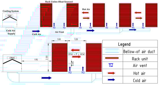
Figure 1.
Detailed thermal configuration of the studied setup.
This problem is considered to represent geometric and physical periodicity. Therefore, A single period will be considered for the analysis. The configuration under study is a rectangular cavity of size H, with its side walls exposed to periodic dynamic and thermal boundary conditions (Figure 2). To replicate heat sinks, two heat sources with a hot temperature (, operational temperature of the heat sink) are mounted on the cavity’s bottom wall. Through two openings of length, convective fresh air is injected from the bottom of the cavity at a temperature of (, fresh air temperature). A long aperture is used on the upper horizontal wall to evacuate the hot air. Air, which is thought to be Newtonian and incompressible and for which the Prandtl number is , fills the enveloping.

Figure 2.
Studied configuration, , , .
Periodic boundary conditions on the vertical walls are applied in order to represent a domain with an extended periodic structure and consistent geometric and flow patterns. This modeling choice is both computationally efficient and physically relevant, as it captures the essential transport mechanisms in systems where lateral effects are negligible. By focusing on a representative periodic unit, the simulation accurately reflects the core behavior of large-scale or modular systems such as finned heat exchangers, microchannel arrays, and porous media where periodicity governs overall performance. This approach ensures that the results are physically meaningful, reliable, and broadly applicable to practical thermal system designs.
The following are the flow fields’ macroscopic governing equations:
where F, , u, p, are the force field, kinematic viscosity, velocity, pressure, and reference density, in that order. The energy conservation equation is expressed as
The scalar variable and diffusion coefficient for the incompressible thermal flows considered in this work are given as temperature T and thermal diffusivity , respectively. The Bossiness assumption is used to include the impact of the temperature field on the flow field. The force field is defined as follows:
where is the reference temperature, j is the unit vector in the vertical direction, g is the gravitational acceleration magnitude, is an external body force, and is the thermal expansion coefficient.
The initial and boundary conditions associated with the problem under study are as follows:
- Initial conditions:
- Dynamic and thermal boundary conditions:
2.2. Cascaded Lattice Boltzmann Method (CLBM)
- The choice of the model
The Cascaded Lattice Boltzmann Method (CLBM) was chosen for this project because it is very good at accurately describing complicated heat flow and transport processes, especially when there is a mix of convection and conduction. Compared to more common methods like finite volume or finite element approaches, CLBM offers better numerical stability, less vulnerability to non-physical oscillations, and an easier way to deal with complex boundary conditions. These features make CLBM perfect for modeling turbulent and transitional flows, like those found in medium- and large-scale heat sinks. Furthermore, CLBM can easily simulate problems on high scales because it is naturally scalable. It does this by using parallel computing to handle the higher computational needs. This advantage makes it an ideal choice for studying the thermal management challenges posed by heat sinks operating under high heat flux conditions.
The D2Q9 lattice model discretizes the dynamic (fluid flow) field, while the D2Q5 lattice model discretizes the thermal field. The D2Q9 model is flexible enough to accurately show the speed distribution and multicellular flow structures that are common in these types of convection. The D2Q5 model is also the best for thermal transport, providing computational economy without sacrificing the precision required for heat transfer computations. This dual-lattice method is a good choice for this study because it makes sure that both the hydrodynamic and thermal fields are resolved correctly and quickly.
- Problem Description and Governing Parameters
In this study, the selected ranges of Rayleigh number () and Reynolds numbers () were chosen to reflect thermal and flow conditions typically encountered in practical applications such as data centers and high-power electronic systems. The Rayleigh numbers correspond to realistic temperature differences (around to ) across air-filled enclosures of decimeter-scale dimensions, which are commonly found in heat-generating equipment.
The Reynolds numbers, on the other hand, represent airflow velocities in the range of approximately 0.5 to 2.5 m/s, consistent with forced convection produced by fans or ducted ventilation systems in such environments. These parameter ranges were selected to ensure that the simulated configurations are representative of real-world mixed convection scenarios and can help identify key behaviors relevant to the design of efficient thermal management systems.
2.2.1. CLBM for the Flow Field
The D2Q9 lattice is used in this study to depict the flow field, which looks at two-dimensional (2D) problems [23]. The lattice space and time steps are represented by the variables ∆x and ∆t, respectively, and the selected lattice speed is . The distinct speeds: are defined by
where the transposition is indicated by the superscript tr, and the column vector is indicated by i = 0 … 8,.
Raw moments and central moments for discrete distribution functions (DFs) fi are provided to build the collision operator based on central moments [24].
The discrete equilibrium distribution function (EDFs), ., is substituted for fi to define the equilibrium values and in an analogous manner. Numerous researchers have adopted the recombined raw moments, k20 + k02 and k20, k02, to treat the trace of the pressure tensor and the normal stress difference independently in literature [25,26,27,28,29,30,31,32]. However, the practical use is time-consuming, especially when dealing with three-dimensional (3D) models.
A simpler approach was presented in [33] to make practical implementation easier. It involved using the raw moments, k20 and k02, and making minor changes to the relaxation matrix. The simplified raw-moment set is used in this study,
and the united key Shifted moments also do . More precisely, M transforms the raw moments from fi via a transformation matrix M and N [30,34] separates the essential moments from the raw moments using shift matrix N. The notation for M and N is as follows:
The expressions used here are simpler and have the potential to lower processing costs when compared to the M and N expressions in [29]. The post-collision central moments are obtained by separately relaxing each central moment to its equilibrium equivalent, as follows:
where Ci are the forcing source terms in central moment space, and the block-diagonal relation matrix is given by
with and . The continuous central moments of the Maxwell-Boltzmann distribution in continuous velocity space are equivalent to the equilibrium central moments of [24],
of resulting in the Cascaded collision operation. The equilibrium Distribution function is defined by the Maxwell–Boltzmann equilibrium distribution function by
where is the fluid density, and is the sound speed on a lattice. A generalized local equilibrium is the analogous EDF [28,29]. The forcing terms in discrete velocity space are expressed by Ning et al. [35] as follows:
In central-moment space, the forcing source terms are uniformly specified as [28,29],
In the streaming step, the post-collision discrete DFs in space x stream to their neighbors x+ along the characteristic lines as usual,
The discrete DFs after a collision are ascertained by To get the Hydrodynamics variables, the following steps are performed:
The current approach utilizes the incompressible approximation [36,37], whereby, i.e., and are the density fluctuations. The incompressible Navier Stokes may be replicated by the Low-Mach number limit by using the Chapman-Enskog analysis [28]. The relaxation parameters are connected to the kinematic and bulk viscosities. by and , respectively.
2.2.2. CLBM for the Temperature Field
In this subsection, a D2Q5 (the five discrete velocity set, , CLBM is proposed to solve the convection-diffusion equation for the temperature field. Similarly, the raw moments and central moments of the temperature distribution functions can be defined by
The simplified raw-moment set (as opposed to the recombined raw-moment set) is also used in the D2Q5 lattice [31]:
Recombined Raw-Moment Set:
Simplified Raw-Moment Set:
And so do the recombined central moments . Analogously, the raw moments and central moments can be calculated through a transformation matrix MT and a shift matrix NT, respectively.
Explicitly, MT and NT are expressed as,
The collision in central moments can also be written as
where is the matrix of diagonal relaxation. A continuous ‘temperature’ equilibrium distribution is developed in the continuous velocity space that is comparable to the Maxwell-Boltzmann distribution ().
where “Sound speed ” is defined. Next, a crucial step is taken by equating the discrete central moments to the continuous central moments :
Consequently, the values in equilibrium may be expressed as
The post-collision temperature distribution functions can be obtained by
The streaming step for also takes the form:
The temperature T is calculated as follows:
3. Computational Implementation
3.1. Heat Exchange
Convective heat transfer in a fluid flow is measured using the global Nusselt number (). The preponderance of convection over conduction is defined by this value. This is one way to describe it:
with
: the height or width of the wall i
: normal on the wall
: the tangential to the wall i
with
: Number of nusselt on the right-hand side heat sink right
: Number of Nusselt on the right-hand side heat sink left
: Number of Nusselt on the left-hand side heat sink right
: Number of Nusselt on the left-hand side heat sink left
: Number of Nusselt of the source horizontal heat sink right
: Number of Nusselt of the source horizontal heat sink left
For example:
3.2. Numerical Meshing
To ensure the reliability of the results, a mesh sensitivity analysis was first carried out for laminar and early transitional regimes, where the flow remains relatively stable and grid convergence can be assessed with good confidence. From this preliminary study, a practical refinement strategy for higher Rayleigh and Reynolds numbers, where the simulations become significantly more demanding in terms of computational cost is derived.
For the same order of magnitude (e.g., from to ), a constant mesh resolution could be maintained without a noticeable loss of accuracy is founded. However, when transitioning to a higher order of magnitude (e.g., from to ), the mesh was further refined to ensure numerical precision and capture the intensified flow structures.
This approach was particularly necessary given the large size of the computational domain, the high values of Rayleigh and Reynolds numbers, and the use of periodic boundary conditions that increase the representativeness of the modeled configuration. These factors substantially elevated computational requirements.
Despite the inability to perform a full Grid Convergence Index (GCI) analysis for all configurations, the adopted strategy guarantees a balance between computational feasibility and numerical accuracy. The selected mesh resolutions provided stable, physically consistent, and quantitatively reliable results throughout the range of parameters studied. Table 1 summarizes the mesh resolutions employed for the various configurations investigated in this work.

Table 1.
Mesh values used for different simulations based on Reynolds () and Rayleigh () numbers.
3.3. Validation of the CLBM Code
The program is verified using a well-known typical design [38,39], which consists of an air-filled square cavity with constant Prandtl number (), adiabatic horizontal walls, and constant temperature ( and ) on the vertical walls. With a maximum difference of , the results in Table 2, which include speeds, stream functions, and Nusselt number values, show a strong match with the reference results. Table 2 below provides a quantitative comparison between the present findings and those reported in the literature.
Table 2.
Comparison of the present results with those reported in the literature for Ra .
Figure 3, given below, compares the flow configurations with a Rayleigh number (). For qualitative validation, we looked at a cavity setup where an isothermal heater sticks out from the bottom wall. There’s also an isothermal partition, with height h and width w, placed at a distance d from the right wall, kept at a constant temperature . The two vertical walls are kept at a cooler temperature , while the top and bottom horizontal walls are insulated.
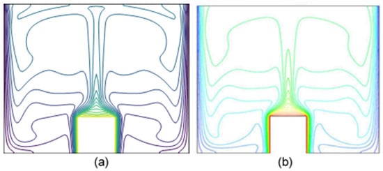
Figure 3.
Isotherms: Comparison of the present results (a) with those of AlAmiri (b) [40,41].
The quantitative validation results are summarized in Table 3, where a comparison of the maximum values of the stream function () and velocity components (, ) was performed, showing a quantitative agreement within a margin of error of approximately 5% with the results of AlAmiri et al. [40,41]. The streamlines are presented on the right, while the isotherms appear on the left. The streamlines are on the right, while the isotherms are on the left. When it comes to streaming, the isothermal structures that are achieved numerically and those that are acquired empirically exhibit extremely good agreement and have similar shapes. The highly developed nature of mixed convective fluxes is evident. In the two structures being compared, the closed cells show natural convection, while the open lines of the stream function show forced convection. The value of represents the maximum of the stream function. As shown in Figure 3 and Figure 4, the findings demonstrate a high degree of agreement with the experiment.
Table 3.
Quantitative comparison between the present work and the results of AlAmiri et al. [40]. for and .
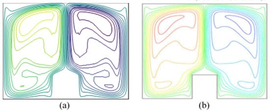
Figure 4.
Flow structures: Comparison of the present results (a) with those of AlAmiri (b) [40,41].
4. Results and Discussion
4.1. Flow Structure and Thermal Fields
4.1.1. Dynamic and Thermal Fields for
The stream function visualization reveals a complex, multicellular flow structure, as indicated in Figure 5. For , (Figure 5a) two convective cells fill the entire space between the heat sinks (hereafter referred to as micro-cavity) by keeping out fresh air. In fact, the air confined in this zone is set in motion by the thermal gradient imposed by the vertical walls of the blocks. As it rises towards the center of the cavity, it is forced to move downwards under the effect of the training by the forced jet on the one hand a cooling in contact with the latter which will increase its density and therefore its weight, on the other hand. Two other low-intensity cells are in the upper part of the cavity. They are a consequence of the interaction between the ambient air (relatively hot) and the jet of forced convection (cold). These cells have a favorable effect on the heat exchange between the cavity and the exterior, since they accentuate the mixing of the two airs and increase the residence time of the fresh air jet in the cavity. The open lines representing the ventilated air have a separation at the horizontal faces of the hot blocks. They are, moreover, distorted in the upper part of the cavity, because of the shear with the drive cells mentioned above. As the Reynolds number increases, the entrainment phenomenon disappears from the top of the cavity, giving way to fresh ventilation air. Only micro-cavity is the seat of closed convective cells, as shown in Figure 5b–d for , ,, respectively. The rotation direction of two cells (in the micro-cavity) permits a part of the fresh air jet to enter the micro-cavity’s core. The right-hand part cools more than the left because of a distortion at the base of the boundary layers and an entrainment cell on the left-hand horizontal section that pushes the jet of fresh air towards the right-hand horizontal section. Consequently, both the horizontal sides of the blocks and the vertical side of the apertures with respect to the micro-cavity experience excellent cooling.
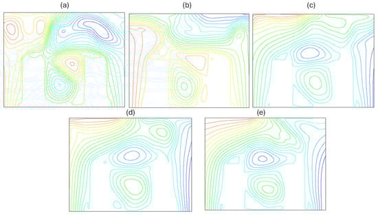
Figure 5.
Streamlines of (a) ; (b) ; (c) ; (d) ; (e) .
The thermal field indicated by the isothermal lines is shown in Figure 6. Generally, the two faces close to the openings are often quite cold. The heat exchange between these two vertical plates and ambient air is quite significant, as shown by the isothermal lines which are too tight indicating a development of thermal boundary layer heat transfer along these plates. For , given in Figure 5a, a small amount of fresh air moves towards the bottom of the micro-cavity, driven by the rotating cells mentioned above. It increases as the Reynolds number increases, relatively improving heat transfer along the vertical faces adjacent to the micro-cavity, Figure 5b, . This phenomenon disappears for up of . Indeed, when increases further, the jet becomes relatively intense compared to the downward drag phenomenon, Figure 5c–e, for , and , respectively. On the other hand, a recirculation of fresh air appears above the hot blocks. Its clockwise direction is favorable to the cooling of the horizontal wall of the right block to the detriment of that on the left. In all cases, these two faces remain the site of poor heat exchange due to the separation of the forced air jet described previously.
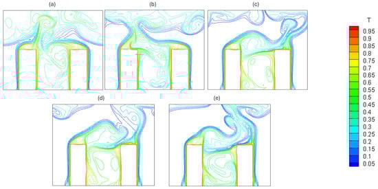
Figure 6.
Isotherms of (a) ; (b) ; (c) ; (d) ; (e) .
4.1.2. Flow and Thermal Fields for
In general, the structure of the flow becomes more complex compared to the case of . The turbulent regime is well established, represented by a multitude of closed cells of different sizes. Among these, two large natural convection cells (Rayleigh-Bénard type) are located above the blocks occupying the entire upper half of the cavity, Figure 7a, for . The jet of fresh air, still weak, bypasses these cells by tracing the long path before leaving the cavity. When the is increased to , the right convective cell is split into two. One is relocated towards the right corner of the cavity and the other is lowered into the micro-cavity, Figure 7b. The more increases, the more the forced jet takes over the convective cells at the top of the cavity and the more air is circulating in the micro-cavity. The competition between the natural convection cells and the forced jet driving the latter to laminate the horizontal walls of the blocks, Figure 7c,d, for and . It is also necessary to mention the appearance of small entrainment cells between the fresh air and the horizontal walls of the heat sinks, shielding against heat transfer for high values of .

Figure 7.
Streamlines of (a) ; (b) ; (c) ; (d) .
The isothermal lines are generally very tight along the vertical walls of the heat sinks. The development of thermal boundary layers is observed in these areas. On the other hand, there is a distortion of the isothermal lines around the hot horizontal walls. The joint effect of the separation of the fresh air jet and the drive keys above them is, surely, the cause of poor heat exchange. For , Figure 8a, it is noted that the lower zones on the left and right of the two blocks are the sites of thermal stratification presented by practically horizontal isothermal lines. The rest of the cavity is the site of distorted and distant lines testifying to a fully turbulent regime. There are also existing closed isothermal lines. They can indicate the existence of warm puffs of air moving in the cavity. As increases, the stratification mentioned above disappears and the lower zones of the cavity (on the side of the fresh air inlets) become isothermal cold, Figure 8b–d.

Figure 8.
Isotherms of (a) ; (b) ; (c) ; (d) .
4.2. Heat Transfer
To thoroughly investigate the heat transfer performance within the cavity, the study follows a structured three-step analysis based on the global Nusselt number . In the first stage, the instantaneous evolution of is computed on all surfaces of the heat sinks for both Rayleigh numbers values ( and ). This step provides insight into the temporal behavior of heat exchange between the solid blocks and the surrounding fluid, particularly under unsteady and transitional regimes. It helps to identify the onset of flow stabilization and the influence of the Reynolds number on the thermal response over time.
In the second stage, averaged global Nusselt number , it enables precise quantification of the net heat transfer rate in the fully developed regime. The average Nusselt number serves as a reliable metric for assessing the impact of forced convection intensity on overall thermal performance.
Finally, the third stage focuses on deriving empirical correlations that relate to the Reynolds number, separately for each Rayleigh number. These correlations provide practical predictive tools for estimating thermal efficiency under similar operating conditions, and they reflect the nonlinear interplay between buoyancy-driven and forced convective effects in transitional regimes.
Importantly, this Nusselt-based thermal analysis complements the physical interpretation of the flow and temperature fields previously obtained from isotherm contours and streamlines. While visualizations offer qualitative insights into flow structures and thermal pathways, the Nusselt number offers a quantitative synthesis, helping to bridge local flow phenomena with global heat transfer performance.
For when analyzing the overall variations in the global Nusselt number alongside the fluid dynamics inside the cavity (see Figure 9), a more physical and intuitive understanding of the heat transfer emerges.
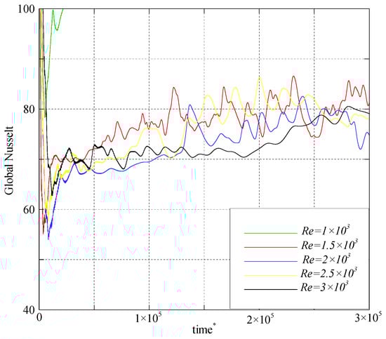
Figure 9.
Time variation of global Nusselt number for different Reynolds Number values, time* denotes dimensionless time, as defined in the nomenclature.
At the beginning of the simulation, for all Reynolds numbers considered, a transient phase is observed, characterized by strong fluctuations in the global Nusselt number. This period corresponds to the gradual establishment of flow and temperature structures within the cavity, with heat exchanges still unstable. Then, for low Reynolds values (up to about ), the global Nusselt number tends to stabilize around an average value, exhibiting only slight oscillations. This reflects a regime still dominated by natural convection, where the air circulates in relatively regular recirculation cells. These structures allow fresh air to reach the bottom of the cavity, locally enhancing cooling. In the thermal field, this is manifested by well-organized isotherms concentrated along the vertical walls near the openings, indicating sustained heat transfer on these surfaces.
However, for , a regime change takes place. The forced air jet becomes strong enough to disrupt the natural flow. More pronounced oscillations appear in the global Nusselt curves, becoming nearly periodic with marked peaks, especially for and . These oscillations are not simply numerical instabilities; they reflect the real competition between two heat transfer mechanisms: the natural convection trying to organize the flow, and the forced convection imposing a dynamic, often unstable jet. The fluid alternates between phases of recirculation and phases dominated by the blown jet, causing the rises and falls in .
Physically, this instability results in the emergence of secondary recirculation zones, notably above the heat sink. These flow structures enable effective cooling of the right block but disrupt the airflow toward the left block, creating an asymmetry in thermal efficiency. These zones, clearly visible in the streamlines, directly influence heat exchange at the walls. Thus, even though the average heat transfer intensity (represented by Nu) generally increases with Re, this improvement is accompanied by significant fluctuations, indicating an unsteady, possibly chaotic regime.
Figure 10 clearly illustrates the influence of the Reynolds number () on the efficiency of heat transfer within the cavity equipped with thermal dissipators. At a lower Reynolds number, specifically , the flow is largely governed by natural convection. This is confirmed by the stream function, which shows two large Rayleigh-Bénard-type convection cells occupying the upper half of the cavity. In this regime, the forced airflow remains weak and bypasses the convection cells along a long path, limiting its direct interaction with the surfaces of the dissipators. As a result, heat transfer remains relatively modest, with the global Nusselt number stabilizing around 100 after the initial transient phase. As increases to , the flow becomes more complex. The right-side convection cell splits, with one part pushed toward the upper right corner of the cavity and the other descending into the micro-cavity (space between the heat sinks). This change reflects a growing influence of the forced jet on the overall flow structure, enhancing the penetration of cooler air into regions near the dissipators. This promotes better surface cooling, thins the thermal boundary layers, and leads to a noticeable increase in the Nusselt number. At higher Reynolds numbers, and , the forced jet becomes the dominant mechanism driving the flow. It suppresses the natural convection cells, pushing them upward, while also penetrating the space between the dissipators. This leads to the streamlines aligning more closely with the surfaces of the dissipators an effect that promotes strong convective heat transfer, with the Nusselt number exceeding 150. However, this strong jet also gives rise to small entrainment cells between the main airflow and the surfaces of the dissipators. These localized recirculations can temporarily reduce the heat transfer in specific regions, which explains the oscillations observed in the Nusselt number at higher .

Figure 10.
Time variation of global Nusselt number for different Reynolds Number values, time* denotes dimensionless time, as defined in the nomenclature.
Overall, the combined analysis of the Nusselt number and the stream function reveals a clear transition from a natural convection-dominated regime to one where forced convection prevails. This shift leads to a significant improvement in heat transfer performance due to the enhanced interaction between the airflow and the dissipator surfaces, despite the presence of small-scale flow instabilities at higher Reynolds numbers.
To really highlight the sensitivity of the heat exchange between the hot block faces and the fresh air, an average value of was defined and denoted as representing the average between the maximum and the minimum of from a time τ chosen according to the value.
The average value of the global Nusselt number was examined as a function of the Reynolds number for . As reported in Table 4, increases from 76 to 86 across the investigated Re range, indicating a clear influence of forced convection on the overall heat transfer. This trend suggests that the flow intensification promotes more effective convective transport, even in the presence of significant buoyancy effects. The confidence interval associated with the slope of the fitted correlation, [0.00274, 0.00358], is relatively narrow, which reflects a consistent and statistically reliable relationship between and . This supports the validity of modeling the variation as a linear function of Reynolds number. The resulting correlation is given by
Table 4.
Values of for different values of , .
With
- regression coefficient
- confidence interval: [0.00274, 0.00358]
For , in the same way, the was studied in the turbulent regime zone, as a function of . Table 5 presents values for different values of considered in this study. As indicated, it varies from 119.22 for till 152.10 for , with a variable growth rate (varying from 0.560 till 0.895), much higher than that relating to the case of .
Table 5.
Values of for different values of , .
The confidence interval for the slope, [0.01941–0.02656], remains relatively tight despite the higher variability, which confirms the robustness and statistical significance of the correlation in this regime.
The evolution of the average value of the global Nusselt number is also linear in this case too, as presented in Figure 11. A correlation is proposed for this relation as follows:
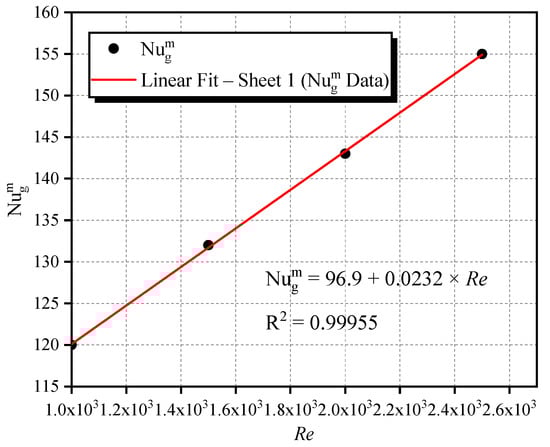
Figure 11.
Evolution of the average global Nusselt number as a function of , .
With
- regression coefficient
- confidence interval: [0.01941–0.02656].
Figure 11 and Figure 12 illustrate the relationship between the average global Nusselt number and Reynolds number () at different Rayleigh number values (). Figure 12 shows that for , the effect of turbulence on heat transfer is moderate, and increases steadily with . In contrast, Figure 11, which corresponds to , highlights a more pronounced influence of convection, leading to a stronger increase in the . This indicates that at higher Rayleigh numbers, natural convection becomes more dominant, and more advanced cooling solutions might be required to maintain optimal temperature conditions in heat sinks. These findings are particularly relevant for thermal management in large-scale systems where both temperature gradients and flow control play a critical role.
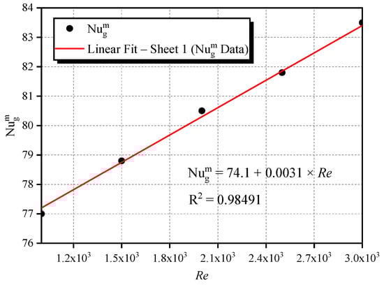
Figure 12.
Evolution of the average global Nusselt number as a function of , .
The correlations between and shown in these graphs tell us a lot about how turbulence and thermal gradients affect heat transfer. They also provide useful predictive tools for engineers to anticipate the thermal behavior under different operating conditions. This knowledge can be used to enhance the design of cooling systems in heat sinks (data centers, electronic components…), leading to improved performance and reduced energy consumption. In particular, these correlations allow for faster thermal assessments during the early design stages, help avoid overdesign, and support decisions on airflow rate and geometry sizing without relying exclusively on costly experimental or high-fidelity simulations.
5. Conclusions
This study used the Cascaded Lattice Boltzmann Method (CLBM) to provide a complete picture of how to control the temperature of medium- and large-sized heat sinks. The trustworthiness of this method has been further supported by the outstanding agreement between benchmark results from the literature and the built and tested numerical code. Reynolds number values between and were investigated, along with Rayleigh number values of and with an emphasis on mixed convection regimes. Due to these parametric ranges, the interaction between forced and natural convection modes in various flow and temperature conditions could be described. The study found that as the Reynolds number goes up, heat moves much faster along the vertical walls of the heat sinks. This is particularly true up to , which is the point where the flow starts to become turbulent (). After this point, the forced air jets’ impact takes over and more effectively shapes the thermal field. The average Nusselt number varies slightly; its value increased by 8.3%, from 76.94 to 83.3, indicating that considerable cooling improvements are possible with regulated airflow. Localized inefficiencies in heat evacuation result from areas of partial air confinement that continue to exist between the heat sinks. The thermal and dynamic fields become much more complex at higher Rayleigh numbers (), which correspond to truly turbulent regimes. Intense mixing and powerful natural convection cells define the flow, greatly increasing the rate of heat transfer. In This case, the average Nusselt number increases significantly in this environment. It went from 199.22 to 152.10, a 27.6% increase, as Re increases. Under very high temperatures, the crucial function of coupled forced and natural convection processes is highlighted by the heat transfer’s marked sensitivity to the Reynolds number. This study helps clarify how heat transfer behavior depends on both thermal loading and flow control, providing insight that can inform real-world cooling system design. In particular, since the Rayleigh number inherently includes the characteristic size of the heat sinks, our analysis also captures how the physical scale of the system influences thermal performance. The flow regimes, thresholds, and derived correlations offer valuable guidance for engineering applications, including airflow control and heat sink sizing. Such correlations derived from CLBM simulations can support predictive design approaches without requiring full-scale parametric optimization. This provides a useful framework for practical implementation in applications such as data centers and industrial cooling modules. By showing that the Nusselt number goes up in direct proportion to the Reynolds number, this connection, which was found through simulations using the CLBM, shows how forced flow improves heat transfer in large heat sinks. This connection makes it possible to find the best configurations for systems in places like data centers or tough industrial settings. It also makes it possible to accurately predict the thermal performance of heat sinks on a large scale. This study proposes correlations for such applications. These results have the potential to solve localized inefficiencies and improve thermal management in high-performance systems.
Author Contributions
Conceptualization, F.Z.L.A. and H.F.; Methodology, E.S., A.G. and A.M.; Software, M.E.A. and E.S.; Validation, F.Z.L.A., M.E.A. and E.S.; Formal analysis, F.Z.L.A. and A.G.; Investigation, M.E.A., E.S., H.F., A.G. and A.M.; Resources, A.M.; Writing—Original draft, F.Z.L.A.; Writing—Review and editing, M.E.A., H.F., A.G. and A.M.; Supervision, M.E.A., E.S. and H.F.; Funding acquisition, H.F. All authors have read and agreed to the published version of the manuscript.
Funding
This research received no external funding.
Data Availability Statement
The original contributions presented in this study are included in the article. Further inquiries can be directed to the corresponding author.
Conflicts of Interest
The authors declare no conflicts of interest.
Nomenclature
| C | Speed [m/s] |
| Propagation speed [m/s] | |
| Sound speed [m/s] | |
| D | Dimension (LBM) |
| The tangential to the wall | |
| particle velocity [m/s] | |
| F | External forces [N] |
| Body force [N] | |
| Distribution function | |
| Distribution function for a set of particles | |
| Equilibrium distribution function | |
| Gravity acceleration [m/] | |
| Energy distribution function | |
| Equilibrium energy distribution function | |
| H | Dimensionless height of the cavity |
| Dimensionless height of the wall | |
| Central moment of order (m, n) | |
| Equilibrium central moment of order (m, n) | |
| Iteration Number | |
| L | Dimensionless length of distance between heat sink |
| Dimensionless length of heat sink | |
| Dimensionless length of extraction opening | |
| l | Dimensionless width of opening for supply air |
| Transformation Matrix | |
| n | Mesh |
| Normal on the wall | |
| N, | Shift Matrix |
| Local Nusselt number | |
| Global Nusselt number | |
| Average global Nusselt number | |
| Number of Nusselt on the right-hand side heat sink right | |
| Number of Nusselt on the right-hand side heat sink left | |
| Number of Nusselt on the left-hand side heat sink right | |
| Number of Nusselt on the left-hand side heat sink left | |
| Number of Nusselt of the source horizontal heat sink right | |
| Number of Nusselt of the source horizontal heat sink left | |
| p | Dimensionless static pressure |
| Prandtl number | |
| Q | Direction (LBM) |
| Rayleigh number () | |
| Reynolds number () | |
| S | Source term |
| T | Fluid temperature [] |
| Reference temperature [] | |
| Hot temperature [] | |
| Cold temperature [] | |
| reference time | |
| dimensionless time | |
| U | Dimensionless speed on ox |
| V | Dimensionless speed on oy |
| Γ | Moment [N·m] |
| q | Dimensionless temperature () |
| Dimensionless cold temperature | |
| Dimensionless hot temperature | |
| Thermal diffusivity [] | |
| Expansion coefficient [] | |
| Density [] | |
| kinematic viscosity [] | |
| Thermal conductivity [W/m.K] | |
| Relaxation factor | |
| Time variation [s] | |
| τ | Dimensionless time |
References
- Adhikari, R.; Beyragh, D.; Pahlevani, M.; Wood, D. A numerical and experimental study of a novel heat sink design for natural convection cooling of LED grow lights. Energies 2020, 13, 4046. [Google Scholar] [CrossRef]
- Chen, H.-T.; Zhang, R.-X.; Yan, W.-M.; Amani, M.; Ochodek, T. Numerical and experimental study of inverse natural convection heat transfer for heat sink in a cavity with phase change material. Int. J. Heat Mass Transf. 2024, 224, 125333. [Google Scholar] [CrossRef]
- Siddiqa, S.; Naqvi, S.B.; Azam, M.; Aly, A.M.; Molla, M. Large-eddy-simulation of turbulent buoyant flow and conjugate heat transfer in a cubic cavity with fin ribbed radiators. Numer. Heat Transfer Part A Appl. 2023, 83, 900–918. [Google Scholar] [CrossRef]
- Ma, X.; Li, C. Lubrication flow law and cooling mechanism considering cavitation in mechanical seals with Rayleigh step pattern. Appl. Therm. Eng. 2024, 258, 124755. [Google Scholar] [CrossRef]
- Zhang, Z.; Wang, J. Conjugate transient flow and thermal analysis of non-isothermal rubber curing process in autoclave system. Int. J. Heat Mass Transf. 2024, 228, 125641. [Google Scholar] [CrossRef]
- Javadzadegan, A.; Joshaghani, M.; Moshfegh, A.; Akbari, O.A.; Afrouzi, H.H.; Toghraie, D. Accurate meso-scale simulation of mixed convective heat transfer in a porous media for a vented square with hot elliptic obstacle: An LBM approach. Phys. A Stat. Mech. Its Appl. 2020, 537, 122439. [Google Scholar] [CrossRef]
- Zhang, X.; Xu, Y.; Zhang, J.; Rahmani, A.; Sajadi, S.M.; Zarringhalam, M.; Toghraie, D. Numerical study of mixed convection of nanofluid inside an inlet/outlet inclined cavity under the effect of Brownian motion using Lattice Boltzmann Method (LBM). Int. Commun. Heat Mass Transf. 2021, 126, 105428. [Google Scholar] [CrossRef]
- Oh, H.; Jo, H.J. Numerical study of turbulent flow boiling heat transfer in structured cooling channels using lattice Boltzmann method with advanced outlet boundary conditions. In Proceedings of the 33rd Conference on Discrete Simulation of Fluid Dynamics, Zürich, Switzerland, 9–12 July 2024; AIP Publishing: Melville, NY, USA, 2025. Available online: https://pubs.aip.org/aip/pof/article/37/1/013349/3330671 (accessed on 13 May 2025).
- Kefayati, G. Lattice Boltzmann simulation of cavity flows driven by shear and internal heat generation for both Newtonian and viscoplastic fluids. Phys. Fluids 2023, 35, 093111. [Google Scholar] [CrossRef]
- Shojaeefard, M.H.; Jourabian, M.; Darzi, A.A.R. Rectangular heat sink filled with PCM/hybrid nanoparticles composites and cooled by intruded T-shaped cavity: Numerical investigation of thermal performance. Int. Commun. Heat Mass Transf. 2021, 127, 105527. [Google Scholar] [CrossRef]
- Yan, G.; Alizadeh, A.; Rahmani, A.; Zarringhalam, M.; Shamsborhan, M.; Nasajpour-Esfahani, N.; Akrami, M. Natural convection of rectangular cavity enhanced by obstacle and fin to simulate phase change material melting process using Lattice Boltzmann method. Alex. Eng. J. 2023, 81, 319–336. [Google Scholar] [CrossRef]
- Abouricha, N.; El Alami, M.; Gounni, A. Lattice Boltzmann Modeling of Natural Convection in a Large-Scale Cavity Heated From Below by a Centered Source. J. Heat Transf. 2019, 141, 062501. [Google Scholar] [CrossRef]
- Abouricha, N.; El Alami, M.; Souhar, K. Lattice Boltzmann modeling of convective flows in a large-scale cavity heated from below by two imposed temperature profiles. Int. J. Numer. Methods Heat Fluid Flow 2019, 30, 2759–2779. [Google Scholar] [CrossRef]
- Abouricha, N.; EL Alami, M.; Souhar, K. Numerical study of heat transfer by natural convection in a large-scale cavity heated from below. In Proceedings of the 2016 International Renewable and Sustainable Energy Conference (IRSEC), Marrakech, Morocco, 14–17 November 2016; pp. 565–570. [Google Scholar] [CrossRef]
- Harizi, W.; Vitali, M.; Corvaro, F.; Marchetti, B.; Chrigui, M. Experimental and numerical study of mixed convection heat transfer in a vented cavity partially filled with a porous medium: Effects of reynolds and rayleigh numbers on Nusselt number and flow regimes. Numer. Heat Transf. Part A Appl. 2024, 86, 5006–5028. [Google Scholar] [CrossRef]
- El Alami, M. Contribution à L’étude Thermique et Dynamique des Ecoulements le Long D’une Paroi non Uniformément Chauffée Dans une Cavité à Grand Nombre de Rayleigh. Ph.D. Thesis, Indian National Science Academy, Toulouse, France, 2025. Available online: https://www.ccdz.cerist.dz/admin/notice.php?id=128900 (accessed on 10 June 2025).
- El Alami, M.; Khabbazi, A.; El Khatib, H.; Javelas, R. Ecoulements au voisinage d’une paroi non isotherme dans une cavité à grand nombre de Rayleigh (Ra~1010): Étude par similitude. Ecoul. Au Voisin. Une Paroi Non Isotherme Dans Une Cavité À Gd. Nr. Rayleigh Ra1010 Étude Par Similitude 1994, 33, 641–648. [Google Scholar]
- Li, Y.; Jin, T.; Wu, S.; Wei, J.; Xia, J.; Karayiannis, T.G. Heat transfer performance of slush nitrogen in a horizontal circular pipe. Therm. Sci. Eng. Prog. 2018, 8, 66–77. [Google Scholar] [CrossRef]
- Han, F.; Jiang, Z.; Chen, H.; Mao, J.; Ding, X. Numerical investigations on the heat transfer characteristics of pin-fin heat sink for power converters in more electric aircraft. Int. Commun. Heat Mass Transf. 2025, 164, 108866. [Google Scholar] [CrossRef]
- Yakut, R. Determining the cooling performance of the optimized nozzle electrospray cooling system with uniquely designed lattice heat sink. Int. J. Therm. Sci. 2025, 215, 109972. [Google Scholar] [CrossRef]
- Teamah, A.M.; Hamed, M.S. Numerical study of electric motors cooling using an axial air flow. J. Fluid Flow Heat Mass Transf. (JFFHMT) 2022, 9, 101–105. [Google Scholar] [CrossRef]
- Vasilev, M.P.; Abiev, R.S.; Kumar, R. Effect of circular pin-fins geometry and their arrangement on heat transfer performance for laminar flow in microchannel heat sink. Int. J. Therm. Sci. 2021, 170, 107177. [Google Scholar] [CrossRef]
- Geier, M.; Greiner, A.; Korvink, J.G. Cascaded digital lattice Boltzmann automata for high Reynolds number flow. Phys. Rev. E 2006, 73, 066705. [Google Scholar] [CrossRef]
- De Rosis, A. A central moments-based lattice Boltzmann scheme for shallow water equations. Comput. Methods Appl. Mech. Eng. 2017, 319, 379–392. [Google Scholar] [CrossRef]
- De Rosis, A. Alternative formulation to incorporate forcing terms in a lattice Boltzmann scheme with central moments. Phys. Rev. E 2017, 95, 023311. [Google Scholar] [CrossRef]
- Lycett-Brown, D.; Luo, K.H. Multiphase cascaded lattice Boltzmann method. Comput. Math. Appl. 2014, 67, 350–362. [Google Scholar] [CrossRef]
- Li, Q.; Luo, K.H. Effect of the forcing term in the pseudopotential lattice Boltzmann modeling of thermal flows. Phys. Rev. E 2014, 89, 053022. [Google Scholar] [CrossRef] [PubMed]
- Lycett-Brown, D.; Luo, K.H. Cascaded lattice Boltzmann method with improved forcing scheme for large-density-ratio multiphase flow at high Reynolds and Weber numbers. Phys. Rev. E 2016, 94, 053313. [Google Scholar] [CrossRef] [PubMed]
- Premnath, K.N.; Banerjee, S. Incorporating forcing terms in cascaded lattice Boltzmann approach by method of central moments. Phys. Rev. E 2009, 80, 036702. [Google Scholar] [CrossRef]
- Fei, L.; Luo, K.H. Consistent forcing scheme in the cascaded lattice Boltzmann method. Phys. Rev. E 2017, 96, 053307. [Google Scholar] [CrossRef]
- Fei, L.; Luo, K.H. Cascaded lattice Boltzmann method for thermal flows on standard lattices. Int. J. Therm. Sci. 2018, 132, 368–377. [Google Scholar] [CrossRef]
- Shah, N.; Dhar, P.; Chinige, S.K.; Geier, M.; Pattamatta, A. Cascaded collision lattice Boltzmann model (CLBM) for simulating fluid and heat transport in porous media: Numerical Heat Transfer. Numer. Heat Transf. Part B Fundam. 2017, 72, 211–232. [Google Scholar] [CrossRef]
- Sharma, K.V.; Straka, R.; Tavares, F.W. New Cascaded Thermal Lattice Boltzmann Method for simulations of advection-diffusion and convective heat transfer. Int. J. Therm. Sci. 2017, 118, 259–277. [Google Scholar] [CrossRef]
- Asinari, P. Generalized local equilibrium in the cascaded lattice Boltzmann method. Phys. Rev. E 2008, 78, 016701. [Google Scholar] [CrossRef]
- Ning, Y.; Premnath, K.N.; Patil, D.V. Numerical study of the properties of the central moment lattice Boltzmann method. Int. J. Numer. Methods Fluids 2016, 82, 59–90. [Google Scholar] [CrossRef]
- He, X.; Shan, X.; Doolen, G.D. Discrete Boltzmann equation model for nonideal gases. Phys. Rev. E 1998, 57, R13–R16. [Google Scholar] [CrossRef]
- He, X.; Luo, L.-S. Lattice Boltzmann Model for the Incompressible Navier–Stokes Equation. J. Stat. Phys. 1997, 88, 927–944. [Google Scholar] [CrossRef]
- BWan, D.C.; Patnaik, B.S.V.; Wei, G.W. A New Benchmark Quality Solution for the Buoyancy-Driven Cavity by Discrete Singular Convolution. Numer. Heat Transf. Part B Fundam. 2001, 40, 199–228. [Google Scholar] [CrossRef]
- Davis, G.D.V. Natural convection of air in a square cavity: A benchmark numerical solution. Numer. Methods Fluids 1983, 3, 249–264. [Google Scholar] [CrossRef]
- AlAmiri, A.; Khanafer, K.; Pop, I. Buoyancy-induced flow and heat transfer in a partially divided square enclosure. Int. J. Heat Mass Transf. 2009, 52, 3818–3828. [Google Scholar] [CrossRef]
- Corvaro, F.; Paroncini, M. An experimental study of natural convection in a differentially heated cavity through a 2D-PIV system. Int. J. Heat Mass Transf. 2009, 52, 355–365. [Google Scholar] [CrossRef]
Disclaimer/Publisher’s Note: The statements, opinions and data contained in all publications are solely those of the individual author(s) and contributor(s) and not of MDPI and/or the editor(s). MDPI and/or the editor(s) disclaim responsibility for any injury to people or property resulting from any ideas, methods, instructions or products referred to in the content. |
© 2025 by the authors. Licensee MDPI, Basel, Switzerland. This article is an open access article distributed under the terms and conditions of the Creative Commons Attribution (CC BY) license (https://creativecommons.org/licenses/by/4.0/).