Optimization of Sensor Positions and Orientations for Multiple Load Case Scenarios

Abstract

This paper focuses on optimizing sensor placement in structures for load monitoring applications. Such applications rely on sensor data to track changes in the structure. Monitoring accuracy relies on proper sensor placement. The goal is to maximize load monitoring accuracy under multiple loading scenarios while the number of sensors is kept smaller than the number of load cases. Building on prior work in which machine learning models predicted loads using only sensor readings without information on load location, this study continues that approach. It demonstrates that prediction models perform better when sensor networks are optimized. The novelty lies in a newly formulated objective function, allowing for optimization of sensor number, positions, and orientations across multiple load cases and measurement types. The goal is to minimize the differences between maximal responses of the structure and detected responses by the sensors (for all possible load cases). The method is validated on a numerical model of a composite structure with 1–3 sensors under seven different load cases. Load predictions from sensors in optimized locations are compared to predictions from measurements of randomly positioned sensors. Statistical comparison proved that the developed methods and algorithms allow us to significantly reduce the prediction errors.

1. Introduction

In SHM (Structural Health Monitoring), measurements are taken continuously in order to monitor the conditions of the structures [1]. The measurement data can help to track changes in material properties, geometry, boundary conditions, and system connectivity, and can be gathered from the sensors [1]. Therefore, the placements and orientations of sensors determine the effectiveness of the SHM system. Despite significant improvements in SHM, problems with sensor placements still exist because of the complexity of structural responses under different loading conditions [2]. Nowadays, integration of FEM and experimental strain results have improved strain measurement precisions for real-time SHM. These advancements are helpful to make advanced cyber–physical systems in SHM, which improve the ability to monitor and respond to structural issues effectively [3,4].

A lot of research has been conducted regarding optimal sensor placements. The Effective Independence (EFI) method and Fisher Information Matrix (FIM) [5] have been used widely. These methods were developed to improve modal identifiability, especially for large and complex structures. Over time, iterative strategies, like the one proposed by Bagirgan et al. [6], have emerged. In the approach the mobile sensors are used adaptively to refine sensor placement based on updated structural models. Wang et al. [7] summarized approaches emphasizing adaptability, robustness, and sensitivity to operational variability. Yi et al. [8] carried out a hybrid optimal sensor placement strategy that combines QR factorization, sequential sensor placement, and a generalized genetic algorithm to determine both the number and positions of sensors. The method uses modal assurance criterion to evaluate sensor layout performance. In addition, Kyung et al. [9] conducted a unified sensor placement framework that integrates modal strain energy, effective independence, and a modified modal assurance criterion. Their approach uses modal reduction to reduce complexity and explores multiple placement methods individually and in combination, offering adaptable sensor layouts validated through numerical tests on a simply supported truss. Furthermore, Xiao et al. [10] introduced a stiffness separation method that partitions large-scale steel truss structures into smaller substructures, dramatically reducing the computational effort required to invert high dimensional stiffness matrices without sacrificing accuracy. They refined the formulation to ensure force-displacement compatibility and demonstrated on space-truss models that isolate subregions, shrink matrix sizes, and speed up damage identification. Furthermore, Xiao et al. [11] applied a partial-model-based variant of this approach to a full-scale long span steel truss bridge. Their method uses local stiffness models rather than a full global model to detect and quantify member damage. By comparing Nelder–Mead and quasi-Newton optimizations, they confirm that using partial models not only simplifies modeling complexity by over 90% but also enables efficient, accurate detection of damage in service bridges. FIM selects the optimal placements of sensors in order to maximize information acquisition [12]. Lee and Eun [12] extended the classical FIM-based method by iteratively adjusting sensor locations between high and low information areas until FIM determinant or trace stabilization, ensuring that each selected sensor location contributed meaningfully to parameter observability. The evolution of sensor placement has been accelerated by multi-objective optimization algorithms. For example, Gomes et al. [13] used multi-objective optimization that combined FIM and mode-shape interpolation to improve sensitivity to structural changes and enhance accuracy of modal shape reconstruction. Genetic algorithms (GAs) in particular have proven effective for navigating the high-dimensional, non-convex landscape of sensor placement [14]. Multi-objective GAs allow the trade-off between competing criteria, such as sensitivity, redundancy, and robustness, to environmental noise, as seen in work by [15,16]. These methods are especially relevant for structures with multiple load cases, where a limited number of sensors must still provide full spatial and modal coverage.

More recently, data-driven and machine learning (ML) approaches have improved SHM systems, especially in contexts where analytical models are either unavailable or insufficient. ML models learn patterns from data, and this offers predictive capabilities in operational environments. Barthorpe and Warden [17] highlight the growing use of ML models not only for load estimation but also as drivers of sensor placement. Different studies show that integrating sensor placement with the sensitivity of ML model can significantly improve prediction accuracy. Semaan [15] conducted a data-driven sensor placement method based on variable importance from ML models. Then, sensor locations are determined to be placed where the model is most sensitive. Cross et al. [16] extended this concept by integrating FEM-based physical knowledge into Gaussian process regression models using physics-informed kernels, mean functions, and constraints. This physics-informed framework has enhanced model generalization and robustness under sparse or previously unobserved conditions.

ML methods can be divided into artificial neural networks (ANNs), Support Vector Machines (SVMs), and Gaussian Process Models (GPMs). ANNs are quite similar to neural structures of the brain and are suitable for mapping complicated, nonlinear functions between sensor measurements and structural conditions. For instance, in [2] GA is applied to optimize sensor locations under varying environmental conditions, and optimal sensor locations are found that provide high damage detection performance (using ML models) as the temperature varies. Prior work [18] showed that ANNs can predict loads using only strain readings without information on force location. SVM is efficient for classification and regression with small datasets. Their kernel-based formulation enables them to generalize well, even in high-dimensional feature spaces. Additionally, GPMs are a Bayesian framework that output probabilistic prediction together with uncertainties. Such models are useful in SHM, with sparse or uncertain data [16,19]. A recurrent Gaussian Process Regression-based approach utilized in the mode shape reconstruction from sensor locations, which were optimized based on structural dynamics data, was also shown in [19]. This represents a change in approach toward hybrid algorithms, which leverage physical insight and statistical learning.

In recent years, machine learning methods have been successfully applied to operational load monitoring. In the previous work of the authors [18], an artificial neural network (ANN) was trained on numerically simulated strain data from a composite panel under various loading conditions, and this enabled load predictions only based on sensor inputs. In addition to this, the authors implemented an ANN on a low power FPGA platform [20], achieving real-time operational load monitoring with significant reductions in computation demand. These studies demonstrate that ANNs can effectively map strain measurements to load related structural conditions, such as stress or failure indicators, across a wide range of load cases. In both studies, neural networks were trained on data generated from finite element simulations. This paper continues that line of research by addressing a key limitation (suboptimal sensor placement) identified in those works. It is shown here that the performance of such machine-learning-based prediction models can be significantly improved when sensor positions and orientations are optimized. By optimizing sensor layout to maximize information capture across multiple load scenarios, the predictive accuracy and reliability of ANN-based load monitoring systems are enhanced. This paper builds upon the earlier findings by integrating sensor optimization into the model development process, thereby strengthening the overall robustness of machine learning applications in structural health monitoring. The practical applicability is where OLM is implemented: airplanes, bridges, pipelines, wind turbines, and underground vehicles for the mining industry [21,22,23].

Previous work by the authors [24] proposed optimizing single sensor placement for a single load case to maximize measurements in 2D structures. Maximizing sensor measurements allows for more accurate load monitoring and can enable the use of lower resolution data acquisition hardware. This study extends that concept to include multiple sensors, multiple load cases, different measured quantities, and 3D structures.

The novelty of the proposed method is that a new idea for objective function was formulated. By minimizing this function, optimal positions and orientations of any number of sensors can be found for multiple load case scenarios. The assumption is that the number of sensors is relatively small compared to the number of possible load cases of the structure. The proposed method was verified on optimization of sensor placement and orientation in an example composite structure under different loading conditions. The optimization was performed assuming two different physical quantities that are measured, strain and temperature. Strain measurements can be implemented in structural monitoring systems (e.g., to find force value and location or maximal stress value in the structure), and temperature measurements can be implemented in a thermal load monitoring system (e.g., to find the highest temperature in the structure, thermal expansion, or thermal stress where heterogenous temperature distribution occurs). Sensor placement optimization is carried out to minimize the difference between measured and actual physical field values in composite structures. A genetic algorithm is used to iteratively select the optimum sensor configuration from candidate locations that can provide the best objective function. In this study, numerical models of composite structure with 1, 2, and 3 sensors (and multiple load cases) are considered.

To validate this work, predictions from optimally placed sensors were compared to those from randomly placed sensors through a feedforward ANN. Simulated measurements from both random and optimized configurations were used as inputs to ANN. Then, it was trained to predict structural load parameters, such as maximum temperature, applied force, and equivalent von Mises stress. The same ANN structure was applied to all the load cases, with no information about load location. Each configuration was subjected to 500 independent training trials. The prediction accuracy was measured using root mean square error (RMSE). For all the cases, optimized sensor placement produced significantly reduced errors and more consistent performance, confirming that sensor placement optimization plays a crucial role in load prediction model effectiveness.

The structure of this paper is as follows: Section 2 gives a description of the optimization problem and explains the objective function and design variables. It also outlines the sensor modeling approach, constraints, and how sensor readings are simulated for strain and temperature cases. Section 3 gives a description of the numerical implementation, including optimization setup and the finite element model. Section 4 shows the sensor placement optimization for several sensor setups with an objective function evaluation. This section also consists of validation, where optimized sensor configurations are compared to random ones. Conclusions and discussions on the implications of the work to structural health monitoring applications are given in Section 5.

2. Materials and Methods

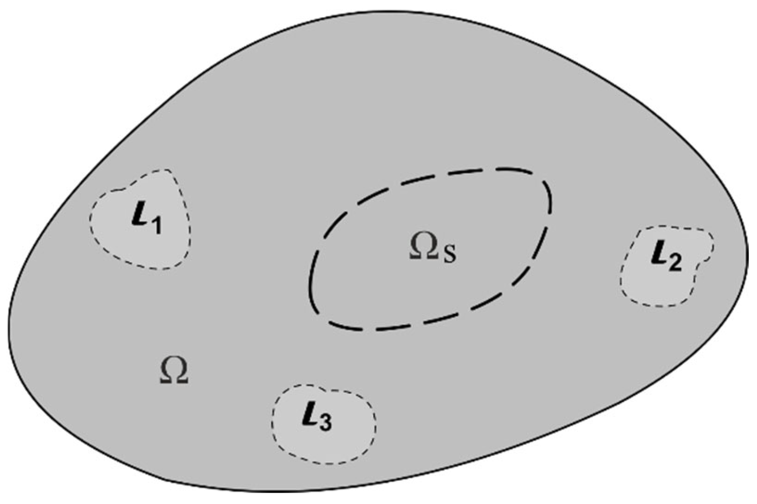
Different load cases produce critical values of measured physical quantities (e.g., strain, temperature, acceleration, displacement, etc.) at different locations of the structure. This situation makes it difficult to accurately capture the exact maximal values for each load case using only a limited number of sensors. Therefore, optimization becomes necessary, as it enables a sensor placement strategy to achieve close approximations of realistic detection results. In sensor placement optimization, the sensor must be placed in some critical area of the structure domain [14,25,26]. As shown in Figure 1, sensors should be placed in key areas of the structure in order to detect the highest strain or temperature and to minimize errors between the detected and actual values. $\mathsf{\Omega }$ is structure domain, ${\mathsf{\Omega }}_{\mathit{s}}$ is the sensor placement area, and ${\mathit{L}}_i$ is the area of applied loads (thermal or structural).

The presented optimization method can be applied to any type of sensor-measured physical quantity. In this paper, two cases are considered: temperature and strain measurements. For each case, the approach for optimization of the sensor positions and orientations is presented. Both approaches utilize a directional interpolation and objective-function minimization approach, where sensor positions and orientations (azimuth and elevation angles) are iteratively optimized to minimize the error between the detected and maximum values (strain or temperature) under various load cases. But, unlike scalar temperature measurements, strain detection is direction sensitive. To account for this, the strain-based model incorporates azimuth and elevation angles, as well as sensitivity coefficients for orthogonal components. This enables more realistic simulation of FBG sensor or strain gage behavior. As a result, sensor orientation can be more accurately optimized, which is critical for capturing the directional characteristics of mechanical strain in 3D structures.

In this study, strain and temperature optimizations were considered separately, but they can be also used together; however, sensors should allow for the separation of both values in computations (for example, the FBG sensor with areas with and without structural loads should be present, or a mix of temperature and strain sensors). The presented approach with separated fields is for clearer validation of sensor placement strategies in each field, where strain is orientation-sensitive and temperature is just scalar. In cases where both mechanical and thermal loads act simultaneously, coupled thermo-mechanical analysis could better capture real-world interactions. The presented decoupled approach provides a controlled way to validate the optimization framework.

2.1. Optimization Problem Formulation

Let the structural domain be denoted by $\mathsf{\Omega }$ and the sensor placement region be ${\mathsf{\Omega }}_{\mathit{s}}\subseteq \mathsf{\Omega }$, as shown in Figure 1. The goal is to optimally place and orient a limited number of sensors within ${\mathsf{\Omega }}_{\mathit{s}}$ such that the difference between the maximum structural response and sensor-detected response is minimized under all load cases.

2.1.1. Design Variables

The design variables are sensor positions and orientations. In 3D structures, for each sensor $j=1, 2,...,m$, the sensor positions are expressed as follows:

$${\mathbf{x}}_{\mathit{j}}=\left(x_{1j}, x_{2j}, x_{3j}\right)\in {\mathsf{\Omega }}_{\mathit{s}}$$

(1)

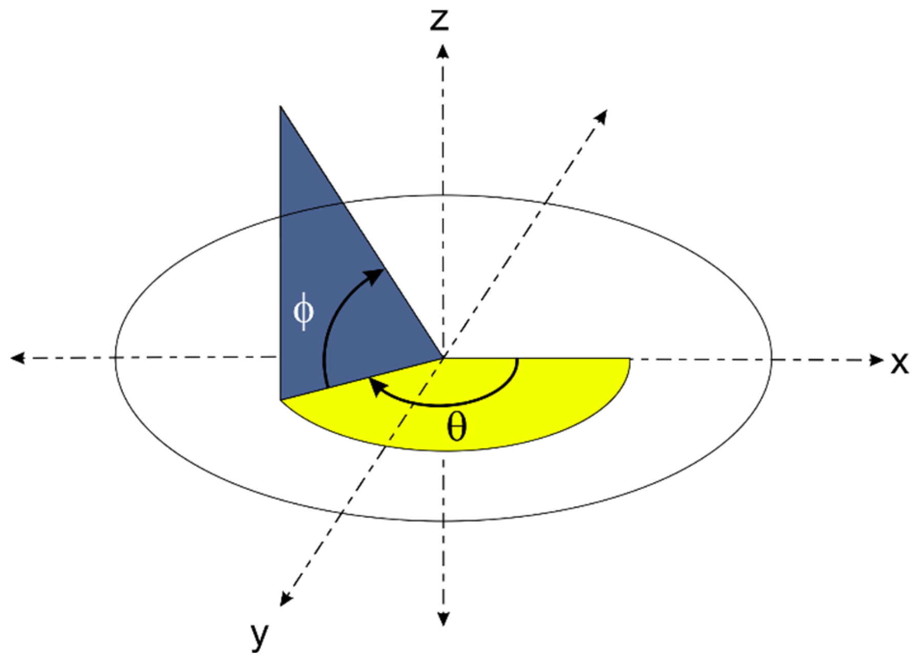
The orientations of the sensors are defined by azimuth ${\mathit{a}}_{\mathit{j}}=\left({\theta }_j, {\varphi }_j\right)$ (see Figure 2).

2.1.2. Constraints

Each sensor position ${\mathbf{x}}_j$ must be located within the designated sensor domain ${\mathsf{\Omega }}_{\mathit{s}}$, which is a subset of three-dimensional space ${\mathbb{R}}^3$. In other words, the position of each sensor is constrained by

$${\mathbf{x}}_j\in {\mathsf{\Omega }}_{\mathit{s}}\subseteq {\mathbb{R}}^3$$

(2)

The orientation of each sensor is defined by the azimuth angle $\left({\theta }_j\right)$ and elevation angle $\left({\varphi }_j\right)$, where the limits are expressed as follows:

$$\begin{gathered} {\theta }_j=\left[0,\pi \right) \\ {\varphi }_j=\left[0,\pi \right) \end{gathered}$$

(3)

The total number of sensors $\left(m\right)$ must be less than the number of load cases $\left(n\right)$. This constraint is applied to avoid redundant or overlapping data.

$$m<n$$

(4)

2.1.3. Sensor Model

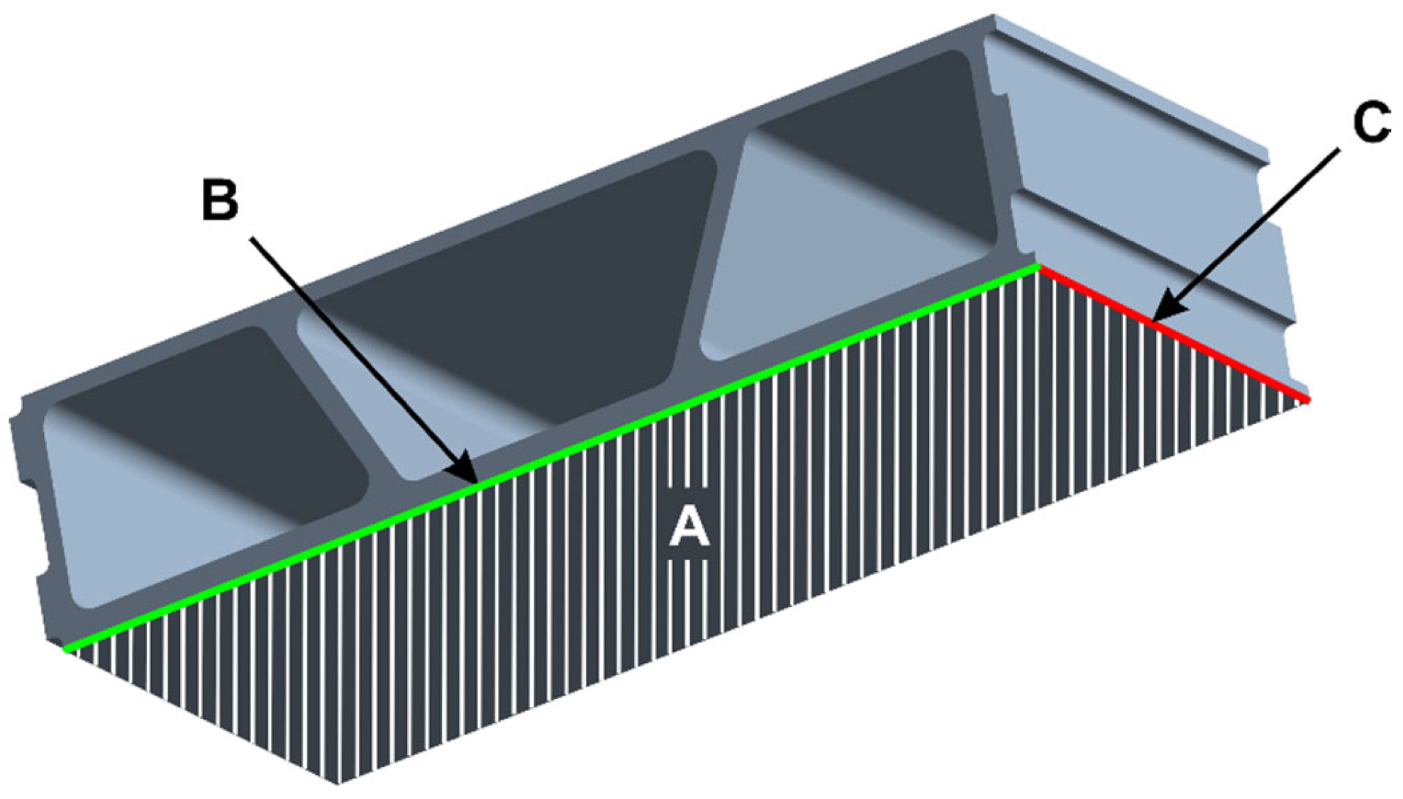
Each sensor j (of center x_j) is modeled as a line in space with two points, $\left({\mathbf{p}}_1\right)$ and $\left({\mathbf{p}}_2\right)$, separated by a distance, $l$, as shown in Figure 3. This line can be created based on azimuth Θ and elevation Φ angles to find the path over which field quantities (in this case strain or temperature) should be evaluated [27]. Azimuth angle Θ is the rotation around x₃-axis (in the x₁x₂-plane). Elevation angle Φ is the rotation around the x₂-axis (in the x₁x₃-plane). Using the trigonometric relations of these angles, one can thus formulate the direction vector d = (d₁, d₂, d₃) such that the line is correctly aligned in 3D space.

$$\begin{gathered} d_1=\cos \left(\Phi \right)\ast \cos \left(\theta \right) \\ {d}_2=\cos \left(\Phi \right)\ast \sin \left(\theta \right) \\ {d}_3=\sin \left(\Phi \right) \end{gathered}$$

(5)

From the original point, the initial and final points of the line are extended along the direction vector multiplied by half of the sensor length. Then, the coordinates of points ${\mathbf{p}}_1$ and ${\mathbf{p}}_2$, which define a sensor, are given by the following:

$$\begin{gathered} {\mathbf{p}}_1=\left({\mathrm{x}}_1+{\displaystyle \frac{l}{2}}\cos \theta \cos \varphi , {\mathrm{x}}_2+{\displaystyle \frac{l}{2}}\sin \theta \cos \varphi , {\mathrm{x}}_3+{\displaystyle \frac{l}{2}}\sin \varphi \right) \\ {\mathbf{p}}_2=\left(x_1-{\displaystyle \frac{l}{2}}\cos \theta \cos \varphi , x_2-{\displaystyle \frac{l}{2}}\sin \theta \cos \varphi , x_3-{\displaystyle \frac{l}{2}}\sin \varphi \right) \end{gathered}$$

(6)

where ${\mathbf{x}}_j=\left(x_{1j},x_{2j},x_{3j}\right)$ are the coordinates of the center of the sensor. These expressions incorporate sensor placement and orientation with respect to structural geometry.

2.1.4. Objective Function

The objective function is used to place sensors such that the differences between the maximal responses (for example equivalent strain or temperature) and detected responses by the sensor are minimized [28]. For this case, the objective function is formulated as follows:

$$f\left({\mathbf{x}}_j,{\theta }_j,{\varphi }_j\right)={\sum }_{i=1}^n{w}_i\underset{j=1..m}{\mathit{min}}\left[{\left(\left|R_{{max}_i}\right|-\left|R_{{det}_i }\left({\mathbf{x}}_j, {\theta }_j, {\varphi }_j\right)\right|\right)}^2\right]$$

(7)

where $n$ is the total number of load cases, m is the number of sensors, $R_{{max}_i}$ is the maximum response of the structure (maximum equivalent strain or temperature) in the domain for the ith load case, $R_{{det}_i }\left({\mathbf{x}}_j,{\theta }_j,{\varphi }_j\right)$ is the value detected by sensor $j$ under the load case $i$, and $w_i$ is the weight of the ith load case that is the inversed maximal response of the structure to the applied load and given as follows:

$$w_i={\displaystyle \raisebox{1ex}{$1$}\!\left/ \!\raisebox{-1ex}{$R_{{max}_i }$}\right.}$$

(8)

To illustrate how to determine the objective function value, let us consider the example structure presented in Figure 4. The number of load cases is n = 3, while the number of sensors is m = 2. For the subsequent load cases where the same amount of load is applied in different locations, the maximal responses of the structure are 3, 5, and 8, respectively. The sensor measurements for each load case are presented in the figure. For this case, the objective function value would be calculated as follows:

$$f={\displaystyle \frac{1}{3}}\min \left[\left(3-2\right),\left(3-1\right)\right]+{\displaystyle \frac{1}{5}}\min \left[\left(5-3\right),\left(5-2\right)\right]+{\displaystyle \frac{1}{8}}\min \left[\left(8-3\right),\left(8-5\right)\right]\approx 1.11$$

(9)

2.1.5. Measured Strains and Temperature Approximation

Due to the finite length of the sensor, it is assumed that the response of a sensor under given load case $R_{{det}_i }$ is the average value of the measured physical quantity at all points on the sensor line within the structure (Figure 5). To simulate it in the objective function evaluation, a finite number of v points is assumed, and the response of the sensor is approximated by the mean value of the responses R_g, where g = 1, 2, …, v.

$$R_{{det}_i }={\displaystyle \frac{1}{l}}\underset{{\mathbf{p}}_1}{\overset{{\mathbf{p}}_2}{\int }}{R}_q\mathrm{d}q\approx {\displaystyle \frac{1}{v}}\sum _{\mathrm{g}=1}^v{R}_g$$

(10)

In the computations of objective function, the $R_{{det}_i }$ values are computed using a numerical model of the structure under load with a relatively dense grid of points with known values of the measured physical quantity for every load case (in this paper, the grid of points of known field values is the mesh of the finite element model). The field values R_g are interpolated using the known values R_k in the set closest points of the nearest data points to g.

$$R_g=\sum _{k\in \mathbf{c}\mathbf{l}\mathbf{o}\mathbf{s}\mathbf{e}\mathbf{s}\mathbf{t}\_\mathbf{p}\mathbf{o}\mathbf{i}\mathbf{n}\mathbf{t}\mathbf{s}}{w}_k{·R}_k$$

(11)

where w_k are weights that are assigned inversely proportional to these distances between points g and k:

$$w_k={\displaystyle \frac{1/({distance}_k+e)}{{\sum }_{j\in \mathbf{c}\mathbf{l}\mathbf{o}\mathbf{s}\mathbf{e}\mathbf{s}\mathbf{t}\_\mathbf{p}\mathbf{o}\mathbf{i}\mathbf{n}\mathbf{t}\mathbf{s}}1/({distance}_k+e)}}$$

(12)

In this interpolation, a very small number $e$ is added to the denominator to avoid division by zero.

2.1.6. Measured Strain Along the Sensor Evaluation

Unlike temperature or other scalar measurements, strain at a point in 3D space in a material can be represented by the strain tensor. Although the primary purpose of a strain sensor is to detect the strain along the sensor, every real-life sensor has some sensitivity to perpendicular strain values. For this reason, a strain transformation method is used to incorporate the impacts of strains perpendicular to the sensor for comprehensive strain detection. The full strain transformation process for a 3D case is shown below. A 3D strain tensor $\mathsf{\epsilon }$ is presented in Equation (13).

$$\mathsf{\epsilon }=\left[\begin{array}{ccc}{\epsilon }_{11}& {\epsilon }_{12}& {\epsilon }_{13}\\ .& {\epsilon }_{22}& {\epsilon }_{23}\\ (\mathrm{s}\mathrm{y}\mathrm{m}.)& .& {\epsilon }_{33}\end{array}\right]$$

(13)

where ${\epsilon }_{11}$, ${\epsilon }_{22}$, and ${\epsilon }_{33}$ are strains along the sensor in $x_1,x_2$, and $x_3$ directions, respectively. ${\epsilon }_{12}$, ${\epsilon }_{13}$, and ${\epsilon }_{23}$ are shear strains in the $x_1{x}_2$, $x_1{x}_3$, and $x_2{x}_3$ planes, respectively.

The transformed strain tensor ${\mathsf{\epsilon }}_{\mathrm{t}\mathrm{r}\mathrm{a}\mathrm{n}\mathrm{s}}$ is obtained using rotation matrix R and original strain tensor $\mathsf{\epsilon }$. In three-dimensional strain transformation, the strain tensor ε in a global (original) coordinate system can be transformed to a new coordinate system using a rotation matrix R. The transformed strain tensor ${\mathsf{\epsilon }}_{\mathrm{t}\mathrm{r}\mathrm{a}\mathrm{n}\mathrm{s}}$ can be expressed as

$${\mathsf{\epsilon }}_{\mathrm{t}\mathrm{r}\mathrm{a}\mathrm{n}\mathrm{s}}={\mathbf{R}}^{\mathrm{T}}\mathsf{\epsilon }\mathbf{R}$$

(14)

where R is a 3 × 3 orthonormal rotation matrix constructed from orthonormal basis vectors d, m, and p. $\mathbf{d}$ is the unit vector in detection of the sensor (see Equation (14)), and $\mathbf{m},\mathbf{p}$ are unit vectors perpendicular to $\mathbf{d}$.

$$\mathbf{R}=\left[\mathbf{d} \mathbf{m} \mathbf{p}\right]=\left[\begin{array}{ccc}{d}_1& m_1& p_1\\ d_2& m_2& p_2\\ d_3& m_3& p_3\end{array}\right]=\left[\begin{array}{ccc}\cos \left(\Phi \right)\ast \cos \left(\theta \right)& -\cos \left(\theta \right)\ast \sin \left(\Phi \right)& \sin \left(\theta \right)\\ \cos \left(\Phi \right)\ast \sin \left(\theta \right)& -\sin \left(\theta \right)\ast \cos \left(\Phi \right)& -\cos \left(\theta \right)\\ \sin \left(\Phi \right)& -\cos \left(\Phi \right)& 0\end{array}\right]$$

(15)

These vectors are used in Equation (13) to extract strain components in their respective directions. The rotation matrix R is used to compute all three components, ${\epsilon }_d,{\epsilon }_m,{\epsilon }_p$, by enabling the following transformation:

$${\mathsf{\epsilon }}_{\mathrm{t}\mathrm{r}\mathrm{a}\mathrm{n}\mathrm{s}}=\left[\begin{array}{c}{\mathbf{d}}^{\mathrm{T}}\\ {\mathbf{m}}^{\mathrm{T}}\\ {\mathbf{p}}^{\mathrm{T}}\end{array}\right]\mathsf{\epsilon }\left[\begin{array}{ccc}\mathbf{d}& \mathbf{m}& \mathbf{p}\end{array}\right]$$

(16)

Expanding this matrix multiplication will give us

$${\mathsf{\epsilon }}_{\mathrm{t}\mathrm{r}\mathrm{a}\mathrm{n}\mathrm{s}}=\left[\begin{array}{ccc}{\mathbf{d}}^{\mathbf{T}}\mathsf{\epsilon } \mathbf{d}& {\mathbf{d}}^{\mathbf{T}}\mathsf{\epsilon } \mathbf{m}& {\mathbf{d}}^{\mathbf{T}}\mathsf{\epsilon } \mathbf{p}\\ {\mathbf{m}}^{\mathbf{T}}\mathsf{\epsilon } \mathbf{d}& {\mathbf{m}}^{\mathbf{T}}\mathsf{\epsilon } \mathbf{m}& {\mathbf{m}}^{\mathbf{T}}\mathsf{\epsilon } \mathbf{p}\\ {\mathbf{p}}^{\mathbf{T}}\mathsf{\epsilon } \mathbf{d}& {\mathbf{p}}^{\mathbf{T}}\mathsf{\epsilon } \mathbf{m}& {\mathbf{p}}^{\mathbf{T}}\mathsf{\epsilon } \mathbf{p}\end{array}\right]$$

(17)

Using the notations for these transformed components

$${\mathsf{\epsilon }}_{\mathrm{t}\mathrm{r}\mathrm{a}\mathrm{n}\mathrm{s}}=\left[\begin{array}{ccc}{\epsilon }_d& {\epsilon }_{dm}& {\epsilon }_{dp}\\ .& {\epsilon }_m& {\epsilon }_{mp}\\ (\mathrm{s}\mathrm{y}\mathrm{m}.)& .& {\epsilon }_p\end{array}\right]$$

(18)

In summary, in 3D space, the strain component in the sensor’s detection direction is calculated using the following expression:

$${\epsilon }_d={\mathbf{d}}^{\mathrm{T}}\mathsf{\epsilon }\mathbf{d}$$

(19)

Expanding this expression, the strain along the sensor can be computed using a quadratic expression that integrates strain tensor and directional vector components.

$${\epsilon }_d={\epsilon }_{11}{d}_1^2+{\epsilon }_{22}{d}_2^2+{\epsilon }_{33}{d}_3^2+2{\epsilon }_{12}{d}_1{d}_2+2{\epsilon }_{13}{d}_1{d}_3+2{\epsilon }_{23}{d}_2{d}_3$$

(20)

In addition to strain along the sensor’s detection direction, some strain sensors (like FBG) may also be sensitive to strain components perpendicular to this direction. Two orthogonal unit vectors, $\mathbf{m}=\left[m_1, m_2, m_3\right]$ and $\mathbf{p}=\left[p_1, p_2, p_3\right]$, define an orthonormal basis together with d. The strain components in these directions, denoted as ${\epsilon }_m$ and ${\epsilon }_p$, are given by the following:

$$\begin{gathered} {\epsilon }_m={\mathbf{m}}^{\mathbf{T}}\mathsf{\epsilon }\mathbf{m} \\ {\epsilon }_p={\mathbf{p}}^{\mathrm{T}}\mathsf{\epsilon }\mathbf{p} \end{gathered}$$

(21)

Expanding these, we obtain

$$\begin{gathered} {\epsilon }_m={\epsilon }_{11}{m}_1^2+{\epsilon }_{22}{m}_2^2+{\epsilon }_{33}{m}_3^2+2{\epsilon }_{12}{m}_1{m}_2+2{\epsilon }_{13}{m}_1{m}_3+2{\epsilon }_{23}{m}_2{m}_3 \\ {\epsilon }_p={\epsilon }_{11}{p}_1^2+{\epsilon }_{22}{p}_2^2+{\epsilon }_{33}{p}_3^2+2{\epsilon }_{12}{p}_1{p}_2+2{\epsilon }_{13}{p}_1{p}_3+2{\epsilon }_{23}{p}_2{p}_3 \end{gathered}$$

(22)

To model the overall strain reading S of a sensor, factors $\alpha$ and $\beta$ are introduced to consider the sensitivity of the sensor towards perpendicular to sensor strain components along m and p, respectively. The total strain reading S is then a weighted sum of strain components in directions d, m, and p:

$$S={\epsilon }_d+\alpha {\epsilon }_m+\beta {\epsilon }_p$$

(23)

Substituting expanded expressions for ${\epsilon }_d$, ${\epsilon }_m$, and ${\epsilon }_p$ we obtain

$$\begin{array}{ll}S={\epsilon }_{11}(d_1^2+\alpha m_1^2& +\beta p_1^2)+{\epsilon }_{22}\left(d_2^2+\alpha m_2^2+\beta p_2^2\right)+{\epsilon }_{33}\left(d_3^2+\alpha m_3^2+\beta p_3^2\right)\\ & +2{\epsilon }_{12}\left(d_1{d}_2+\alpha m_1{m}_2+\beta p_1{p}_2\right)+2{\epsilon }_{13}\left(d_1{d}_3+\alpha m_1{m}_3+\beta p_1{p}_3\right)\\ & +2{\epsilon }_{23}\left(d_2{d}_3+\alpha m_2{m}_3+\beta p_2{p}_3\right)\end{array}$$

(24)

For each load case, strain detection by sensor is calculated as the integral of strain along its length, using the interpolated values of the strain tensor. The average of these strain values provides the representative strain measurement along the line, which corresponds to the detected strain $\left({\epsilon }_{det}\right)$. Considering that ${\epsilon }_q=S$ is strain at point $q$ along a sensor, Equation (9) for the strain takes the following form:

$${\epsilon }_{{det}_i}={\displaystyle \frac{1}{l}}{\int }_{{\mathbf{p}}_1}^{{\mathbf{p}}_2}{\epsilon }_q\mathrm{d}q\approx {\displaystyle \frac{1}{v}}\sum _{\mathrm{g}=1}^v{\epsilon }_g$$

(25)

2.1.7. Simulating Temperature Measurements

In the case of temperature distribution-based sensor placement optimization, the optimization methods focus on minimizing the difference between maximal in the structure $\left(T_{max}\right)$ and detected temperature $\left(T_{det}\right)$ under different load cases.

In order to determine $T_{{det}_i}$, no tensor operations are needed. First, a line that represents the sensor can be made using the sensor’s position and orientation angles to compute direction vector d and define the start and end points of the measurement path. The line is then discretized into several (v) points, and in these points, temperature values are interpolated from surrounding temperature data in the given load case, using Equations (10) and (11). Finally, to obtain $T_{{det}_i}$ the interpolated temperatures along the line are averaged as follows:

$$T_{{det}_i}={\displaystyle \frac{1}{l}}\underset{{\mathbf{p}}_1}{\overset{{\mathbf{p}}_2}{\int }}{T}_q\mathrm{d}q\approx {\displaystyle \frac{1}{v}}\sum _{\mathrm{g}=1}^v{T}_g$$

(26)

2.2. Optimization Algorithm

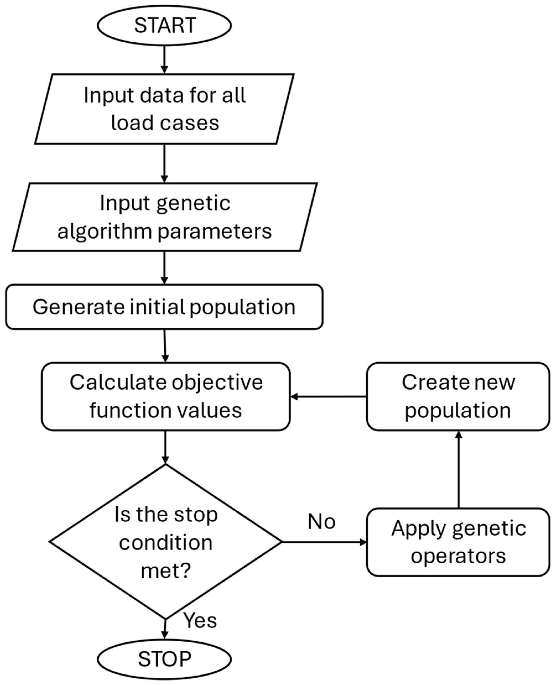
Optimization of sensor placement is explained by the flowchart shown in Figure 6. It starts by obtaining the input data that defines the structural loading cases. It consists of field data (e.g., strain tensors, temperature fields) for all the load cases. The field data is given in the form of values in a dense grid of points, together with coordinates of those points. Next is the configurations of the genetic algorithm. In this case, the key parameters are population size, number of generations, mutation rate, and crossover rate. These parameters determine how the optimization process evolves across iterations. A set of candidate sensor configurations is randomly generated during initial population generation. Each individual in the population specifies a sensor’s 3D position and its orientation. The objective function value is calculated for each individual in the population. First, each sensor is modeled as a line segment in three-dimensional space. The orientation of the line can be determined using azimuth and elevation angles. The sensor line is divided into a number of discrete points. These sample locations simulate the continuous field interaction along the sensor’s physical extent and are used in subsequent interpolation. Using the inverse distance weighting (IDW) method, the algorithm interpolates field values at each sampling point along the sensor line, whether it is tensor or scalar data. A conditional operation determines whether the field type is tensor or scalar. If tensor, the system calculates both parallel and perpendicular components using transformation equations. If scalar, it just computes the average value along the sensor line. The objective function for each individual is calculated. Check stop criteria is defined as the maximum number of generations or minimum error threshold. In following step the genetic operators are applied, and the crossover and mutation create new individuals. A new population of individuals is created. Some of the individuals from the previous generation survived (succession) and some are replaced with new ones during the selection process. When the stop criteria are satisfied, the algorithm selects the best individual and outputs the final sensors’ configuration with an objective function value.

3. Numerical Example

In this study, a structure made of a composite matrix with 50% glass fiber and polyester is considered as the numerical example. The material consists of the properties shown in

Table 1. The material properties used in the numerical example.

Parameters	Values	Units
Young’s modulus	13,000	(MPa)
Poisson’s ratio	0.30	-
Thermal conductivity	0.94060	(W/m°C)

. A fine mesh consisting of 20-noded hexahedral elements was used in the FEM model shown in Figure 7.

The geometrical dimensions of a composite structural model are shown in Figure 8.

For strain-based optimization, the displacement boundary conditions are applied on the bottom side of the structure (Figure 9) as follows: zero displacement (A) was applied to the surface labeled ‘A’ to constrain movement along the x-axis, zero displacement (B) was applied to the edge marked ‘B’ to constrain movement along the y-axis, and zero displacement (C) was applied to the edge marked ‘C’ to constrain movement along the z-axis.

Seven load cases are considered in which the loads are applied perpendicularly to relatively small areas on the top side. The locations are presented in Figure 10.

FEM Data and Sensor Placement Area of the Structure

In this study, ANSYS Workbench 2022 R2 was used to simulate the composite structure [29]. The load case data used in the optimizations were obtained from FEM computations. The composite structure was discretized into about 130,000 (20-noded hexahedral) elements (see Figure 7), resulting in a total of about 600,000 nodes with strains or temperature values for each parameter under every load case. In strain-based optimization, the strain tensors were evaluated for each load case.

From the FEM results, it has been determined that the maximal values of equivalent strains or temperatures are obtained from the shaded area of the structure shown in Figure 11. Therefore, the shaded area of the structure was considered for sensor placement optimization.

Figure 12 and Figure 13 show the behavior of the composite structure when seven different mechanical and thermal loadings are applied. In Figure 12, each load case, with the same 100 N force, has a unique strain field and maximum strain location depending on the load position. This spatial variation shows the extent to which strain responses are localized and also directionally sensitive, due to complex interactions among the material geometry and boundary conditions. Some fields appear highly localized near the point of force application, while others demonstrate more diffuse heterogeneity of elevated strain, indicative of differences in stiffness of the loading path. The asymmetry in some of the distributions suggests stiffness gradients induced by geometry. Generally, there is no one point at which the samples experience peak strain in all the cases, validating the main point of this study. Placement of the sensor should sample those areas that involve multiple candidates for the maxima instead of one fixed spot. This is especially important since our strain sensor model is orientation sensitive, and thus positioning and angular alignment are critical factors to be considered.

Figure 13 illustrates the map of the temperature distribution under applications of the Dirichlet boundary condition of 50 °C to the same locations. Another Dirichlet boundary condition of 25 °C was applied to the bottom surface. To all the other surfaces, a Neumann boundary condition was applied, assuming zero heat flux. Such thermal fields show a high gradient in the region around the heated zones, with maximal values of the temperature near the sources and decreasing values close to the fixed temperature boundary. The evolution of these temperature fields is controlled by the thermal conductivity of the material and by the boundary conditions, in particular by the insulating sidewalls that reduce the lateral heat flow and favor that in the vertical direction. Some load cases present more localized hot spots, while others show larger thermal traces, probably depending on the nearness of the edges or thermal response heterogeneity of the composite. While temperature is a scalar quantity and has none of the directional complexity of strain, capturing peak values still requires optimal sensor placement and correct response characteristics due to the change in position of the maxima. Similarly, temperature peaks are not co-located across cases, just as the strain field, which highlights the importance of distributed sensors. The difference between these two types of fields supports the approach even more: optimized strain sensors must consider both spatial and angular considerations, while temperature sensor placement is based on accurate mapping of the scalar maxima. The FEM results shown in Figure 12 and Figure 13 confirm that optimized sensor configurations based on field-aware criteria are necessary for robust structural monitoring in varying load conditions.

4. Results

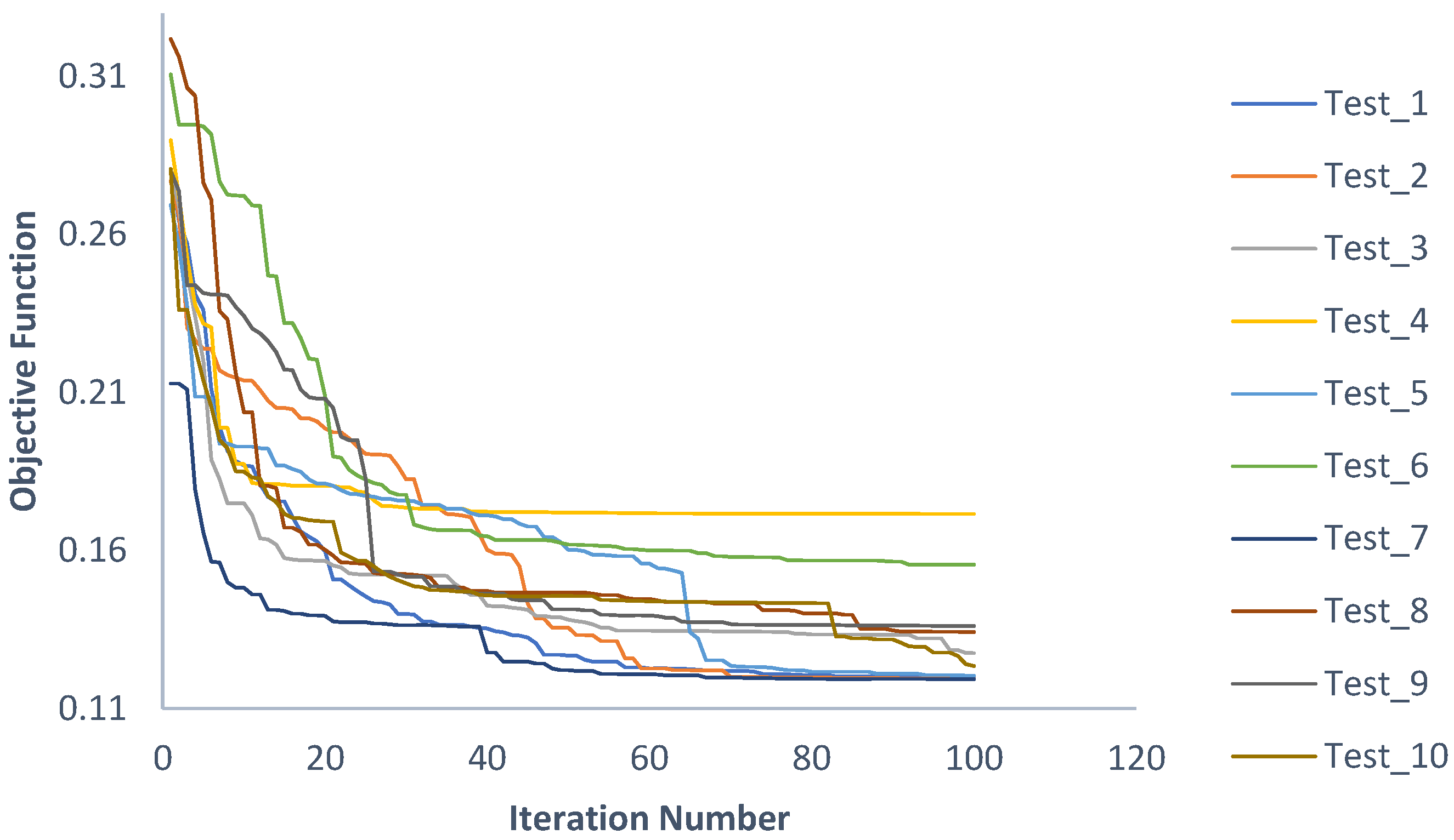
The optimization of sensor placements for strain and temperature distribution monitoring was carried out using genetic algorithms for different numbers of sensors: single, dual, and triple configurations. For each configuration, ten independent optimization runs, each consisting of 100 generations, were performed. In this example, the values of the elevation angles ${\varphi }_j$ are not provided, as this parameter was constrained to zero in order to eliminate the sensor orientation out of structural domain (sensors are placed on a flat surface).

The number of sampling points along the length of a sensor was set to v = 20 (see Equation (9) and Figure 5). The small number e (Equation (11)) was set to 10⁻⁶.

The sensitivity coefficients α and β, used in the strain model to take into account perpendicular strain components, are based on the literature data. The values depend on sensor type, size, and material and are defined by sensor producers. Nowadays, foil strain gauges are characterized by a very low sensitivity for the transverse strain, less or equal to 1% for the sensitivity in the axial direction, as explained in [30]. The grid geometry and manufacturing for such gauges led to a nearly identical response in orthogonal directions (α ≈ β). According to the engineering practice outlined in [31,32], we consider α = β = 0.01. For FBG sensors the sensitivity can be negative or positive up to a few percent [33].

Obtained Results for Different Numbers of Sensors

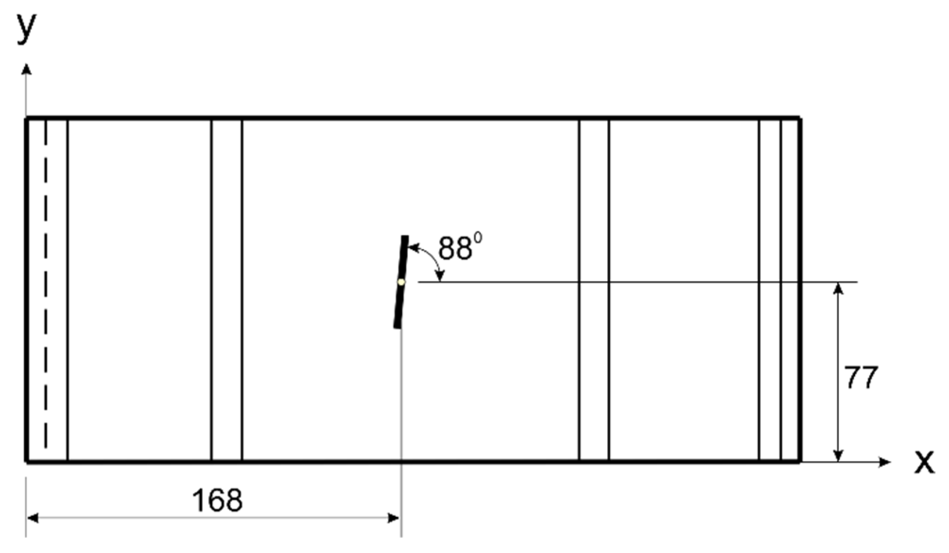
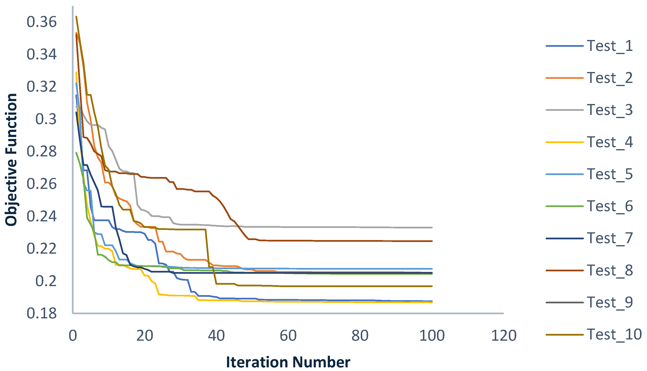
In the strain-based optimization with a single sensor, the best objective function obtained was 0.27, and this was achieved at a coordinate (168, 77, 74) mm with an orientation angle of 88°. The optimal placement and orientation are illustrated in Figure 14, and the convergence performance across the tests is shown in Figure 15.

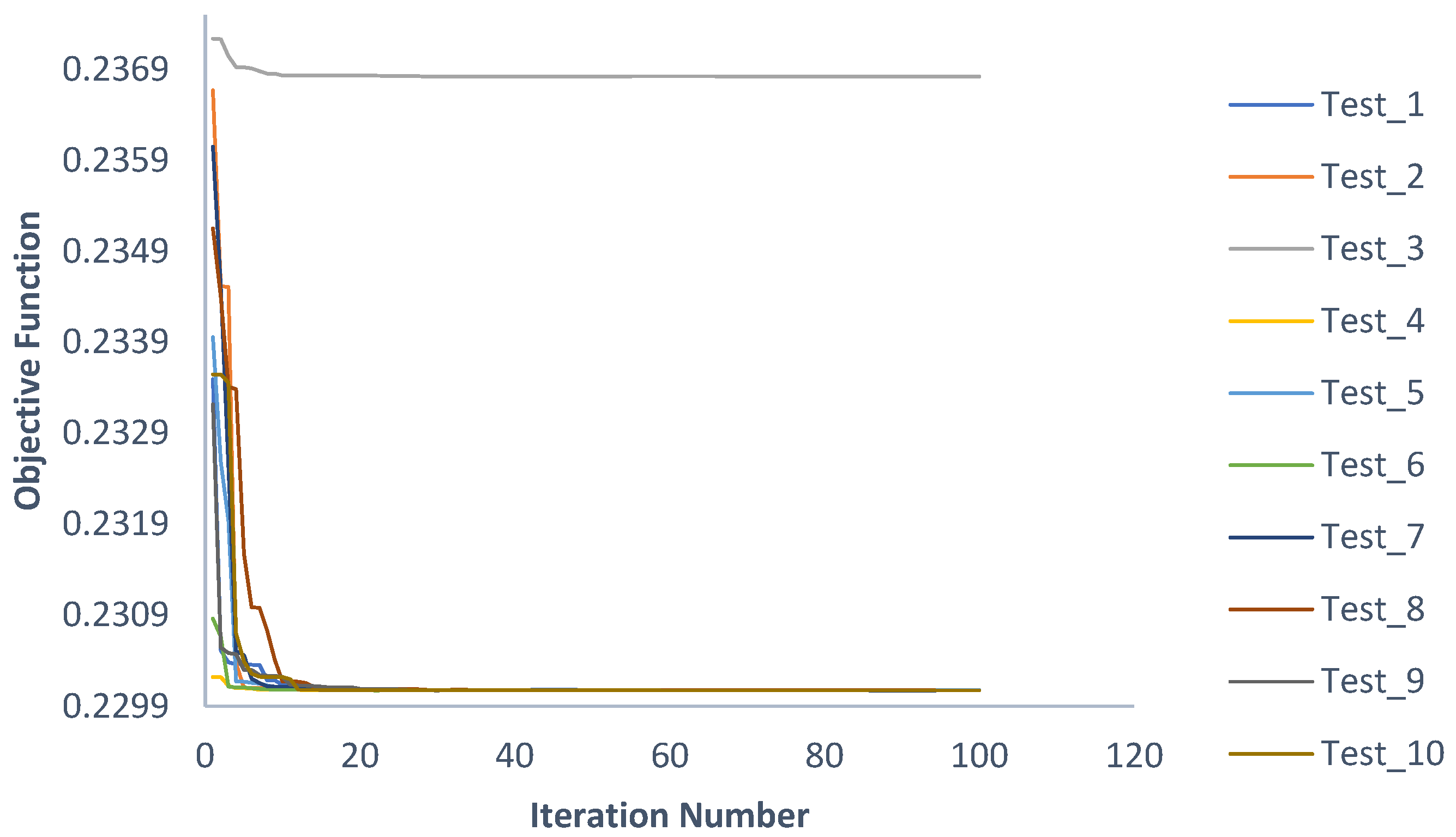
In temperature distribution-based optimization for a single sensor, the minimum objective function recorded was 0.23. This result was achieved with the optimal coordinate and angle of (164, 77, 74), 66°. The results are presented in Figure 16, and the convergence data for the tests is shown in Figure 17.

For the optimization based on strain distributions, the best objective function for two sensors is 0.18. The optimal placement coordinates are (170, 75, 74) mm and (300, 41, 74) mm, with optimal orientations of 88° and 110°, respectively, as shown in Figure 18. The graphs of the independent tests for this case are presented in Figure 19.

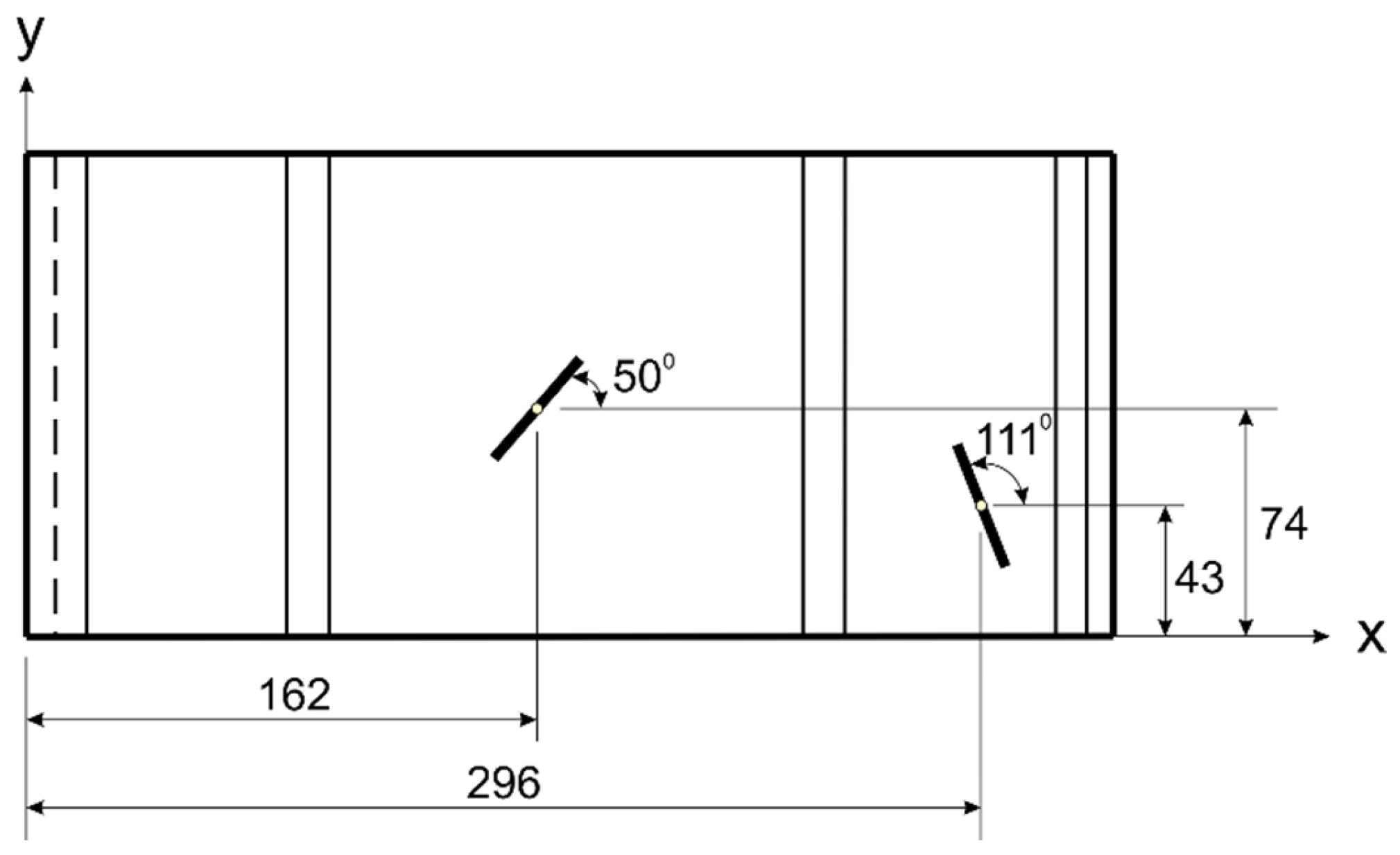
In temperature distribution-based optimization, the best objective function achieved using two sensors is 0.17. The optimal sensor placements are (162, 74, 74) with the optimal angle of 50° and (296, 43, 74) with the optimal angle of 111° shown in Figure 20. Furthermore, Figure 21 shows how evolutionary algorithms converge for two sensor placements in the temperature distribution case.

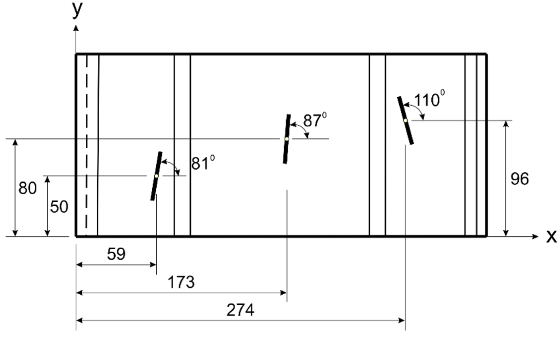
Based on the findings of this work, the optimizations using three sensors provided the best objective functions. For the strain-based optimization, the best objective function value was 0.12. The optimal coordinates and corresponding orientation angles for each sensor are (173, 80, 74) mm at 87°, (59, 50, 74) mm at 81°, and (274, 96, 74) mm at 110°. The optimal coordinates and orientation of the sensors used in this optimization are shown in Figure 22, and the behavior of the genetic algorithm convergence for the three strain-based sensors are shown in Figure 23.

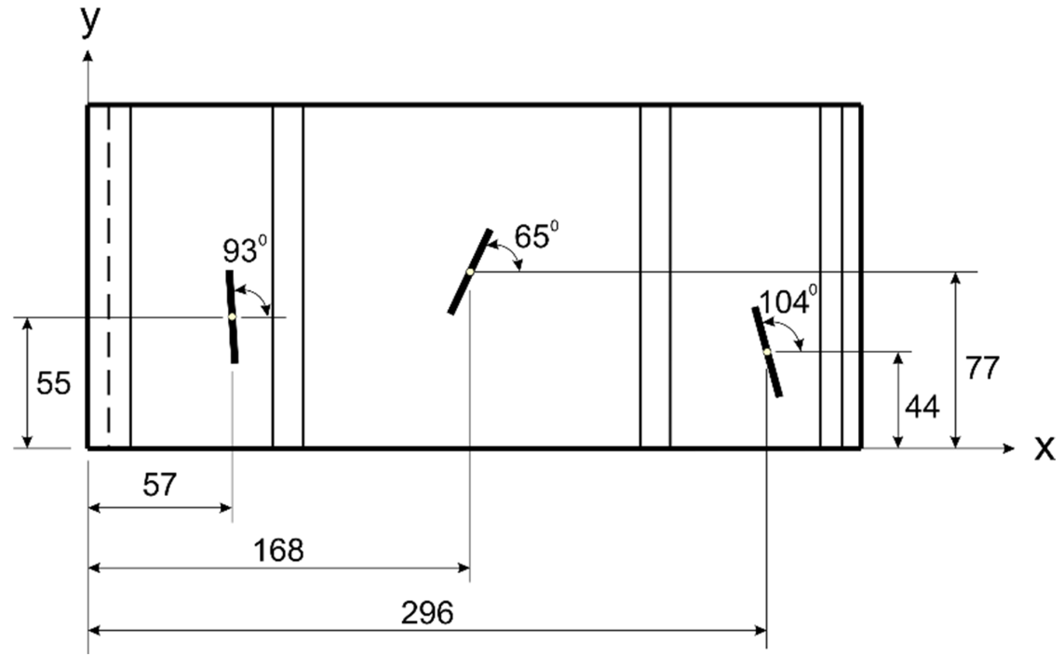
In the temperature-based optimization using three sensors, the objective function attained is 0.12. To find this result, the algorithm determined the optimal placements at (168, 77, 74) mm, (57, 55, 74) mm, and (296, 44, 74) mm, with respective angles of 65°, 93°, and 104°. These optimal coordinates and angles are illustrated in Figure 24, and the test chart for this case is shown in Figure 25.

The results clearly demonstrate the effectiveness of increasing the number of optimally placed sensors in improving monitoring accuracy for both strain and temperature fields. For both types of optimizations, the objective function decreased as the number of sensors increased. The decrease in objective function shows improved coverage and detection capability. This illustrates that multiple optimally placed and oriented sensors can better capture the maxima across different load cases. But it is important to note that the number of sensors must be less than the number of load cases because if there are more sensors, this leads the sensors to capture similar or overlapping data [7,34].

In strain-based optimizations, the result obtained based on a single sensor placement is acceptable. But the two- and three-sensor configurations improved the result more, and this highlights the benefits of spatial diversity and directional complementarity. Similarly, temperature distribution-based optimization showed a significant reduction in objective function, from 0.23 with a single sensor to 0.12 with three, showing the critical role of comprehensive thermal field sampling.

5. Results Validation

The developed sensor placement optimization methodology and algorithms were validated numerically by comparing the accuracy of structural load predictions using simulated sensor measurements, where the sensors are placed in their optimal positions and orientations, against analogous predictions, with sensors in random positions and orientations.

In previous research [35], different ML models were compared for the considered application (operational load monitoring), taking into account their accuracy and computational time. Four different types of ML models (of optimized hyperparameters) were considered: ANNs, adaptive neuro-fuzzy inference systems (ANFIS), support-vector machines (SVMs), and Gaussian processes for machine learning (GPML). The accuracy of predictions was measured and was of the same order of magnitude for each model. GPML and ANFIS turned out to be less accurate and more computationally demanding than the SVM model. The ANN was about 3.4 times faster than the SVM. 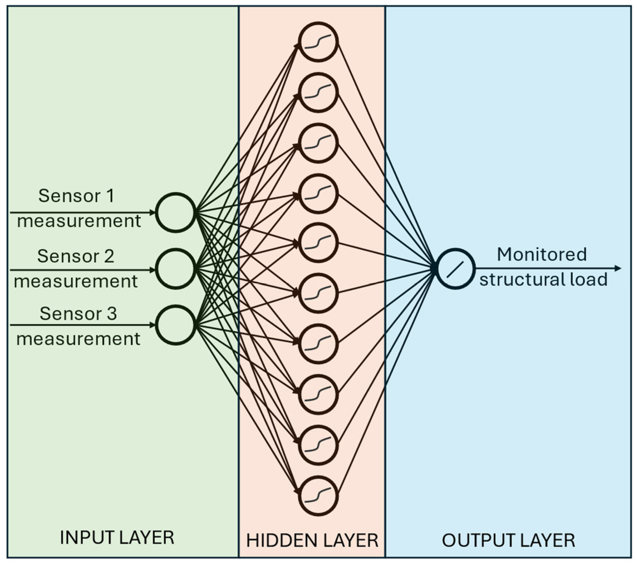For this reason, the feedforward artificial neural network presented in Figure 26 is considered the prediction model here, in the validation.

In the validation process the optimal solutions concerning three sensors are considered. Therefore, the network has three inputs—the measurements of the sensors (temperature or strain). There is one hidden layer with 10 neurons of sigmoid activation function and one neuron in the output layer with linear activation function. The single output of the ANN is considered the monitored load value. In the case of the temperature loads and sensors, the output is the maximal temperature in the entire structure. In the case of force loads and strain measurements, two cases are considered, where the output is either the force value applied to the structure or maximal equivalent von Mises stress in the entire structure. The whole point is that the single prediction model should operate for all load cases without the information of the current load location.

In the validation procedure, the accuracy of the predictions of the ANN is statistically compared for two cases: for 500 training trials, where the sensor locations and orientations are random each time (considering the same constraints as in the optimization process), and for 500 training trials, where the positions and orientations of the three sensors are fixed to the obtained optimal values. There are seven load cases, and for each load case, 100 reference input–output data in the considered load range were prepared using a Latin hypercube sampling plan. This resulted in 700 reference data points. For each training trial a random 70% of the reference data was considered as training, 15% as validation, and 15% as testing data. The Levenberg–Marquardt algorithm was utilized for training.

5.1. Validation of Optimization Results for Temperature Sensors

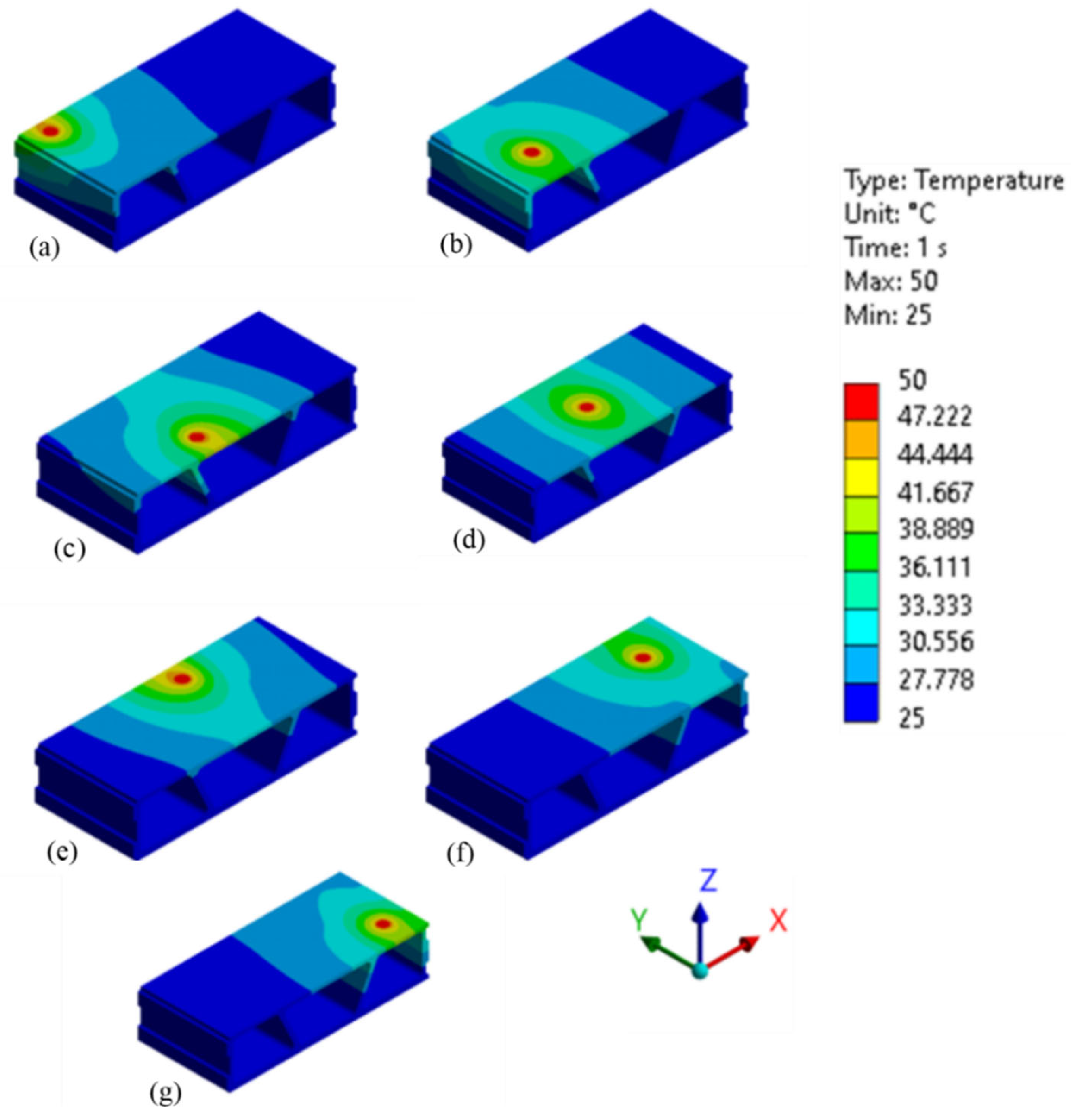
In the validation process of optimization of the positions and orientations of the temperature sensors, the considered monitored load is the maximal temperature value in the whole structure. The load range of the Dirichlet boundary condition between 0 and 50 °C for each load case location is considered.

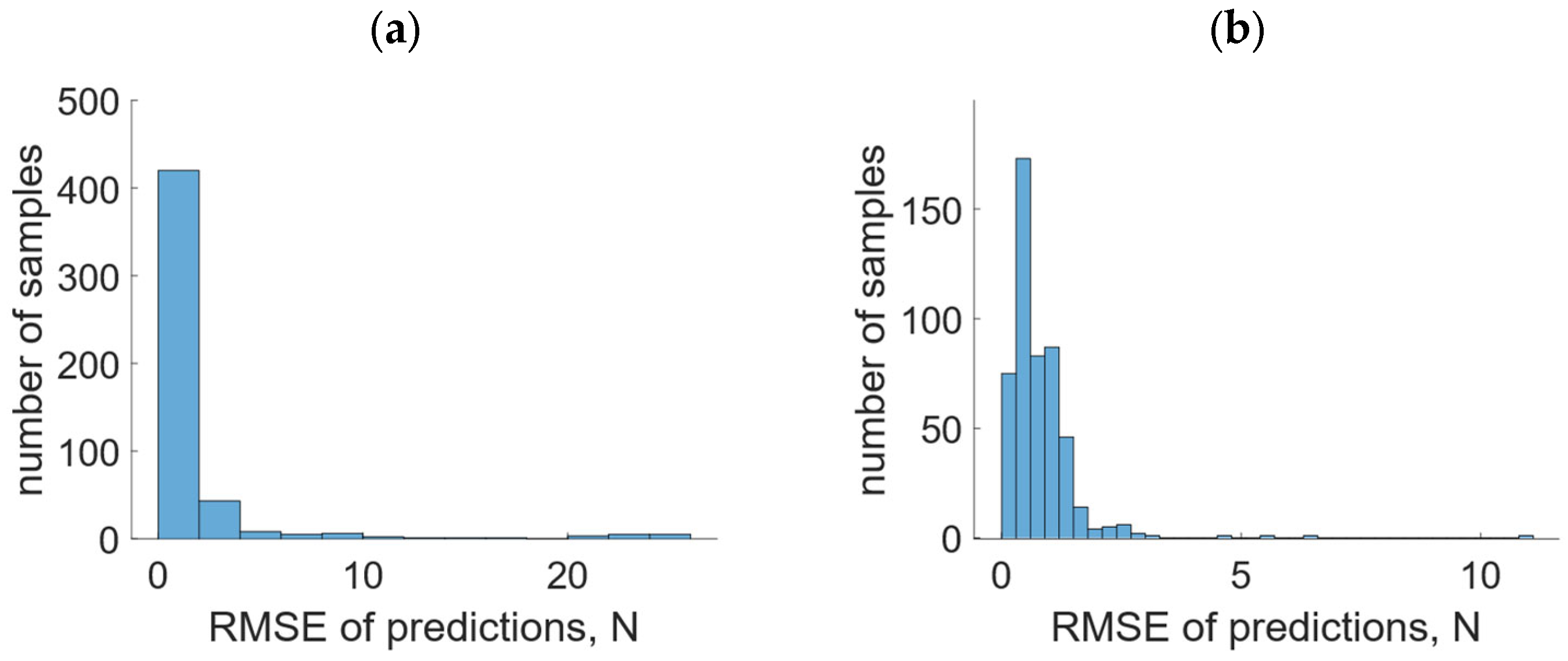
For each of the 500 training trials of the temperature prediction model, the root mean square error (RMSE) between the predictions and targets for all the reference data was calculated. Statistical comparison between the accuracy of prediction models based on measurements from sensors in random positions and orientations against sensors in their optimal positions is presented in

Table 2. Statistical comparison of prediction accuracy of 500 training trials of temperature prediction model based on sensor measurements with sensors in random and optimal positions and orientations; all values in °C.

Title 1	Random	Optimal
Minimal value	0.0076	0.0052
Maximal value	3.0844	0.3101
Average	0.2115	0.0198
Standard deviation	0.4854	0.0201

. The minimal value of all the trials for optimal positions is lower than the minimal value for random positions. The maximal value, average value, and standard deviation for optimal positions is lower than the corresponding values for random positions by an order of magnitude. The histograms of RMSE for all the training trials for both cases are presented in Figure 27. The results prove that the aim of the implemented optimization method was achieved, as it allowed us to obtain a prediction of much greater accuracy than positioning the sensors randomly.

5.2. Validation of Optimization Results for Strain Sensors

In the validation process of the optimization of positions and orientations of the strain sensors, two cases of the monitored load are considered: the applied force value and maximal von Mises stress in the whole structure. The range of the applied force for each load case location is between 0 and 100 N. Taking into account 100 N of force, the maximal values of equivalent stress in the whole structure are 3.2011 MPa, 3.6225 MPa, 3.5078 MPa, 4.8768 MPa, 4.7679 MPa, 3.6656 MPa, and 3.6778 MPa, respectively, for LC1–LC7. The locations of maximal stress for load cases LC1–LC7 are identical to the maximal values in the equivalent strain maps in Figure 12.

Statistical comparison of the accuracy of the force prediction models was prepared analogously to the comparison of the temperature prediction models and is presented in

Table 3. Statistical comparison of prediction accuracy of 500 training trials of force prediction model based on sensor measurements with sensors in random and optimal positions and orientations; all values in N.

Title 1	Random	Optimal
Minimal value	0.1916	0.1178
Maximal value	25.8922	11.0801
Average	1.8495	0.7993
Standard deviation	3.9720	0.7761

. All the statistical measures are lower for optimal sensor positions than random sensor positions. Moreover, the mean value and standard deviation is lower by an order of magnitude. The histograms are presented in Figure 28. This proves that sensor positions have great influence on prediction accuracy, and the optimization has brought desirable results.

The second case of predictions from the strain measurements concerned maximal equivalent von Mises stress in the entire structure. The statistical measurements of RMSE for all the training trials for both random and optimal sensor positions are listed in

Table 4. Statistical comparison of prediction accuracy of 500 training trials of stress prediction model based on sensor measurements with sensors in random and optimal positions and orientations; all values in MPa.

Title 1	Random	Optimal
Minimal value	0.0054	0.0042
Maximal value	0.8523	0.2814
Average	0.0667	0.0261
Standard deviation	0.1285	0.0216

. Once again, all the measurements are lower for the optimal solution. The histograms of RMSE are compared in Figure 29. For optimal sensor placement, the RMSE range is narrower, and the bars are closer to zero than in the case of random sensor placement.

6. Conclusions

This study considered optimization of sensor placements for strain and temperature field monitoring using genetic algorithms. The methodology was applied to configurations of one, two, and three sensors, for both strain-based and temperature-based monitoring. In all the configurations, increasing the number of optimally placed sensors improved monitoring accuracy, as indicated by the progressive reduction in objective function values from 0.27 to 0.12 for strain-based, and from 0.23 to 0.12 for temperature-based monitoring.

The best sensor positions not only provided enhanced spatial coverage but also considered the detection direction sensitivity of the sensors. This shows the importance of both position and orientation in maximizing structural health monitoring effectiveness. The genetic algorithms converged towards an optimal solution within a practical number of iterations. The presented framework constitutes a scalable, data-driven, and computationally efficient approach to improve sensor-based load monitoring. The limitation is that this method does not optimize the number of sensors.

The optimization method was further validated by evaluating its influence on the precision of load predictions from artificial neural networks. Prediction models trained with sensor data from optimally placed and oriented sensors showed a substantial improvement over models using randomly placed sensors. For 500 training trials, the RMSE in prediction of temperature, applied force, and von Mises stress were consistently and significantly reduced when optimal configurations of the sensors were used. In all the cases, the average error and variability were dropped, even by an order of magnitude, which confirmed that the optimization method significantly improves prediction precision across different load conditions without requiring knowledge of the load location.

The developed methods and algorithms, as well as the obtained results are considered by the authors as a starting point for future research, including the following directions: (a) experimental verification of load predictions based on optimal sensor network for multiple load cases; (b) introducing multi-objective optimization of the sensor placement for maximization of the prediction accuracy and minimization of the number of sensors; (c) defining and solving an optimization problem that allows us to find minimal number of temperature and strain sensors and their optimal mutual positions in thermomechanical coupled problems.