An Efficient Parallelization of Microscopic Traffic Simulation

Abstract

Large-scale traffic simulations at a microscopic level can mimic the physical reality in great detail so that innovative transport services can be evaluated. However, the simulation times of such scenarios is currently too long to be practical. (1) Background: With the availability of Graphical Processing Units (GPUs), is it possible to exploit parallel computing to reduce the simulation times of large microscopic simulations, such that they can run on normal PCs at reasonable runtimes?; (2) Methods: ParSim, a microsimulator with a monolithic microsimulation kernel, has been developed for CUDA-compatible GPUs, with the aim to efficiently parallelize the simulation processes; particular care has been taken regarding the memory usage and thread synchronization, and visualization software has been optionally added; (3) Results: The parallelized simulations have been performed by a GPU with an average performance, a 24 h microsimulation scenario for Bologna with 1 million trips was completed in 40 s. The average speeds and waiting times are similar to the results from an established microsimulator (SUMO), but the execution time is up to 5000 times faster with respect to SUMO; the 28 million trips of the 24 h San Francisco Bay Area scenario was completed in 26 min. With cutting-edge GPUs, the simulation speed can possibly be further reduced by a factor of seven; (4) Conclusions: The parallelized simulator presented in this paper can perform large-scale microsimulations in a reasonable time on readily available and inexpensive computer hardware. This means microsimulations could now be used in new application fields such as activity-based demand generation, reinforced AI learning, traffic forecasting, or crisis response management.

1. Introduction

Simulating the individual door-to-door trips of an entire active population is feasible, even for large urban areas, with today’s computers. A virtual copy of the real population, called the synthetic population, is becoming a reality thanks to the availability of big data, large random access memories, and faster microprocessors. Modeling the interactions between neighboring vehicles or between vehicles and pedestrians results in precise trip times and speed profiles, allowing accurate performance evaluations and transport impact analysis. This is a major advantage enabling accurate assessments, including (1) evaluating the sustainability analysis of various transport policies in what-if scenarios, e.g., additional transport services, new vehicle types, or road network modification can be realistically integrated in the model; (2) testing emergency and evacuation scenarios where specific parts of the transport network are blocked or fail; and (3) testing the performance and impact of new vehicle technologies on a large-scale.

There are principally two downsides of microsimulations: (1) the modeling can be resource intensive, as many details need to be modeled in the right way, otherwise even smaller modeling errors may lead to catastrophic consequences and a complete distortion of the results; (2) there is a long execution time with respect to classical flow-based traffic assignment methods—this is the main reason why microsimulations are not used in Activity Generation, traffic forecasting, and many other time-critical applications. This paper addresses the speed issue of current microsimulators and shows that with the use of Graphical Processing Units (GPUs) and adequate parallelization this drawback can be almost entirely overcome.

1.1. State of the Art

Conventional, flow-based traffic assignment methods have been invented to determine traffic flows in larger urban road networks; see [1] for a comprehensive overview. These assignment problems could be solved with the limited computing power available during the 1960s and 1970s. The representation of individual vehicles or even pedestrians in large-scale scenarios (e.g., with thousands of vehicles and people) only became feasible with increasing computing power and memory size at the turn of the century. Different open-source projects such as TRANSIMS [2] and SUMO (Simulation of Urban MObility) [3,4] or commercial software such as VISSIM [5], AIMUSUN [6], or DRACULA [7] have been developed. Microsimulation models are typically very detailed, including lanes (with individual access-rights, speed-limits, and widths), different intersection types (priority, stop, etc.), and traffic-light systems (TLSs) with different traffic-light logic (TLL) and different TLS control strategies. Vehicles are essentially represented by the vehicle-following model, which includes driver behavior and a lane change model [3]. The computation time for large-scale microsimulation scenarios is typically slower than real time [8]. In many applications, traffic assignments run in a loop, for example, during an activity plan generation [9] or user-equilibrium assignment [10]. If thousands of simulation runs are required, such as in AI-reinforced learning [11], then the simulation of a single run should complete in a fraction of the real time.

One possibility for simulating individual vehicles at higher speeds is the use of mesoscopic simulators, which use dynamic First Input, First Output (FIFO) queues as a basic edge model. FIFO queues are widely used in transportation, as these queues preserve the order in which vehicles enter and leave the queue. In contrast with microscopic simulations, mesoscopic simulations do not reproduce speed profiles because the vehicles in the queue are not coupled through vehicle following models. The mesoscopic simulation platforms MATSIM [12] or JDEQSIM are used to generate or calibrate agent-based and activity-based demand models [13]. JDEQSIM is the simulation engine of the Behavior, Energy, and Autonomy Modeling (BEAM CORE) platform [14], where agents can also change plans and routes during the simulation. JDEQSIM has parallelized some algorithms, for example, queuing-events or routing can be processed in parallel by different cores on the CPU [14]. Also, SUMO and other microsimulators have the ability to multithread for dedicated tasks; for example, the core simulation and routing [15].

However, none of the established microsimulators exploit the possibility to distribute the computational burden across thousands of GPU cores. One reason may be that it takes considerable effort to migrate from the serialized algorithms implemented for CPUs to parallel algorithms suitable for GPUs.

There have been several attempts to create microsimulators for GPUs from scratch instead of migrating from an existing code base: the simulator “Microsimulation Analysis for Network Traffic Assignment” (MANTA) [16,17] was later integrated into a larger framework called Large-scale multi-GPU Parallel Computing based Regional Scale Traffic Simulation (LPSim) [18]. LPSim is a discrete time–discrete space simulator, which means that the speeds and positions of all active vehicles are updated during each simulation step, where one simulation step advances the simulation time by a regular time interval. The vehicle positions are discrete, as the lanes of the road network are subdivided into lane-cells of 1 m length, where a lane-cell corresponds to one byte on the GPU’s memory. If a cell is occupied by a vehicle, then the cell-value corresponds to the speed of the respective vehicle; otherwise, it defaults to 255. This means that the space is discretized in 1 m sections and the speed is discretized in 1 m/s steps. The vehicle update basically includes three distinct processes: (1) the car following model (LPSim uses the IDM model [19]), where each vehicle adjusts its speed to a lead vehicle in front or accelerates to the maximum allowed speed if there is no vehicle ahead; (2) the lane-change model, where the vehicle changes lane if the vehicle gap on the target lane is sufficiently large; a vehicle would only change if the lane change is necessary to turn into the successive edge (mandatory lane-change); discretionary lane changes seem not to be modeled at the reported development state; and (3) intersection model, where vehicles change to the successive edge on their pre-determined route; particular care is taken to prevent the simultaneous occupation of lane-cells by multiple vehicles trying to merge into the same edge; this is accomplished using atomic operations, which are also used in the present work and discussed in Section 2.3.3. The traffic light model is greatly simplified, where red lights at junctions flash at a regular pace and vehicles stop during red phases.

The execution speed of LPSim/MANTA is three orders of magnitude faster than SUMO for comparable simulation tasks [16], which means that the advantage of parallel simulator implementation is quite evident. The validation results have shown that LPSim reproduces realistic speed profiles and trip distance distributions [18]. This means that microsimulations could already substitute for the previously mentioned mesoscopic simulations in the calibration, relaxation, and optimization loops used to generate activity-based demand models, as used in many studies of large-scale areas [20,21]. It is worth mentioning that MANTA also includes an optimized routing algorithm that updates link travel times during routing. This algorithm runs in parallel on multiple CPU cores is able to route 3.2 million OD pairs in 62 min. Clearly, routing time has not been included in simulation time, as routing is considered a separate task.

Compared with other microsimulators, one must state that LPSim is neither an event-driven cellular automata [22] nor a discrete-time, continuous state simulator, such as most single-core microsimulators. Instead, LPSim uses updates at discrete times and discrete state variables (e.g., position, speed), in contrast to most single-core microsimulators, which are discrete in time and continuous in vehicle states. The adopted space and speed discretization may provide a sufficient resolution in most cases, but low-speed vehicle movements (e.g., during congestion) could result in an artificial stopping of all involved vehicles, leading to backpropagating queues and gridlock. The use of one byte per cell to store speed information limits the speed of all vehicles to a maximum of 254 m/s, which does not restrict applications to urban or extra-urban environments. However, the GPU memory usage of LPSim seems to be an issue; the 24 h Bay Area scenario (for details, see Section 3.1) appears not to fit on a single GPU with 40 GB of memory. This is why LPSim adopted a mechanism that enables the simulation to run on multiple GPUs by subdividing the network and distributing vehicles accordingly. However, data communication between GPUs, necessary to synchronize and exchange vehicles, seems to be a bottleneck, depending on the network-load [18].

1.2. Objectives

Despite the impressive performance improvements demonstrated by microsimulators running on GPUs, there is ample room for improvements: (1) The parallelization and respective algorithms can be designed to reduce the execution time. GPUs are structured in arrays of blocks, and data exchange within a block is an order of magnitude faster than the data exchange with the global memory of the GPU. Executing the entire simulation step with a single kernel is another approach to boost simulation speed. (2)  The memory usage can be reduced such that even large-scale applications with several million trips can run on a single GPU. In the case of LPSim, the San Francisco simulation used up to 8 GPUs for a simulation of 24 million trips, which requires a complex and time-consuming exchange of information between GPUs during the simulation runs. (3) The discretization of space and speed could be avoided to improve the results when resolving the discrete-time vehicle following algorithm.

The objective of this paper is (1) to propose a discrete-time, continuous state microsimuator called ParSim that uses a different architecture and parallelization approach with respect to LPSim/MANTA and (2) to demonstrate its effectiveness in terms of speed, accuracy, and memory usage.

The paper is structured as follows: Section 2 describes the basic architecture of the software and explains the most relevant processes; Section 3 shows the simulation results and execution-times and validates the GPU-based simulation against two SUMO microsimulation models: the City of Bologna, Italy, and the San Francisco Bay Area, California; and Section 4 discusses the results, draws relevant conclusions, outlines potential applications for the presented simulator, and suggests further improvements.

2. Architecture and Processes

The proposed ParSim simulator is a time-discrete and space-continuous simulator, where the position and speed of active vehicles are updated on the GPU during each step, which corresponds to a fixed simulated time of $T_S$ seconds. The main features of ParSim and the differences compared to MANTA/LPSim are summarized in

Table 1. Main features of ParSim compared with MANTA/LPSim.

Feature	ParSim	MANTA/LPSim
Time	Discrete, typically 0.5 s	Discrete
Position	Floating point	1 m resolution
Velocity	Floating point	1 m/s resolution
Multiple-GPU	No *	Yes
Kernel implementation	Single kernel fusion	Multiple ***
Lane model	Spread †	Mandatory maneuvers ††
Traffic lights (TLs)	Edge based TL programs	Simplified TL **

* Not needed, even scenarios with tens of millions of trips run on a single GPU. ** Flashing red lights to mimic delays. *** Kernels launched with bootloader to reduce kernel loading time. ^† Traffic spread over multiple lanes to increase edge capacity; no lane changes. ^†† Realistic lane changes with gap acceptance for mandatory maneuvers.

.

Section 2.1 outlines the vectorized architecture of the data representing the network, while Section 2.2 highlights the representation of vehicles. Additionally, Section 2.3 describes the GPU-based architecture of the parallelized microsimulator.

2.1. Network and Traffic Lights

The network model is composed of arrays that characterize the network edges, as depicted in Figure 1a. The network arrays stored in the global GPU memory are summarized in

Table 2. Arrays of the global memory.

Domain	Arrays
Vehicle states	Position, speed, edge and segment index, lane index, route pointer, route array, odometer, and leader references.
Network	Segment lengths, geometry vectors, offsets, speed limits, and forward edge tree.
Control structures	Route matrices, lane queues, vehicle-linked lists, red-light masks, and occupancy maps.
Traffic control data	Timers, phase indices, and program offsets for each traffic light.

.

The edge is represented by vectors that contain information about length, the number of lanes, and maximum allowed speed. Each edge is divided into smaller geometrical segments, which are described by the vectors representing offsets, lengths, and angles, respectively. This information is used to determine the coordinates of all vehicles in the network. Each edge contains one or multiple indexed lanes that are parallel to the edge geometry. Vehicles run on either of them from the start to the end of the edge; the current simulator does not contain a lane-change model to allow for overtaking, for example.

Traffic-light systems, of any complexity and extension, can be modeled: the principle is that during a red phase, a traffic-light logic (TLL) can block the exit of dedicated edges. TTLs are again defined by vectors, representing the phase durations and the index of blocked edges during each phase. However, lane-specific traffic lights, for example, for dedicated left or right turns, are currently not implemented.

This network architecture is sufficiently memory efficient to allow even larger urban areas to fit in the memory of a single widely available GPU.

2.2. Vehicle Model

Vehicles are represented by arrays such as position and speed which are stored in the global GPU memory, see Table 2 for a detailed list.

These vehicle states are updated during each simulation step, based on the lead vehicle behavior and constrained by red lights and its position on the current edge and segment. Each vehicle follows a route, which is a sequence of network edges.

The vehicle control follows the following basic principles: (1) The vehicle’s acceleration is governed by the Intelligent Driver Model (IDM) [19], which allows the driver to achieve a desired speed, as well as to maintain a safe target headway to the lead vehicle ahead. The used control parameters are shown in

Table 3. Used variables for the IDM (according to [19]).

Parameters	Variable	Value
Maximum acceleration	a	2.5
Desired deceleration	b	1.8
Target time headway	$\tau$	1.5
Minimum spacing	$s_0$	3.0
Length of the vehicle	l	5.0
Acceleration exponent	$\delta$	4.0

. (2) If the vehicle does not “see” a lead vehicle ahead, then the desired speed of the vehicle is set to the minimum of the allowed edge speed and the maximum vehicle speed. (3) In case a leader is assigned, the vehicle tries to converge to a desired time headway to the leader, and the desired speed is the speed of the leader. (4) In case the leader changes speed abruptly, such that the following vehicle would “crash” into the leader when applying the acceleration from the IDM model, then the follower would instantly adapt to the speed of the leader, regardless of the acceleration this maneuver may cause; this means the follower cannot crash into or overtake its leader. This is an important property as it prevents data inconsistencies.

When a vehicle surpasses the end of a segment, it gets place on the next road segment. When a vehicle has arrived at the end of the edge, there are three cases to consider: (1) The vehicle looks into the next edge on its route and checks if there is a sufficiently large gap to allow a safe transition to the next edge; in case the next edge has multiple lanes, then the lane with the largest initial gap is chosen; if a sufficiently large gap has been found, then the vehicle transitions to the next edge and looks at the last vehicle on the chosen lane of the next edge. (2) If no sufficiently large gap can be found on either lane of the next edge, then the vehicle does not transition but stops instantly. (3) If the current edge is controlled by a TLL and the edge is in a red phase, then the vehicle will see a “ghost leader” at zero speed, positioned at the end of the edge. The ghost leader is a vehicle that is generated by the algorithms to make simulated vehicles adapt their speed or stop—it is used to set a dynamic or static target.

A synchronization algorithm has been put in place, attempting to sequentialize those vehicles running on edges that converge toward the same junction: if a vehicle, positioned on any of the incoming edges, reaches a predefined distance from the downstream junction, then it is appended to a common FIFO queue and the previously last vehicle in the queue becomes the new leader of the newly entered vehicle. This means that the order in the queue ultimately defines the sequence in which the vehicles cross the junction. The implemented synchronization technique ultimately avoids the deadlocks at intersections that occur with other microsimulators [23], leading to artificial congestion. However, if the incoming edges of a junction are not sufficiently long, then abrupt and unrealistic deceleration do occur, as there is not enough room for the necessary speed adaptations.

2.3. Parallel Execution Model

GPUs are able to execute a vast number of threads in parallel. The software library PyCUDA 2025.1 is utilized to implement the simulator. PyCUDA is a Python 3.10.0 interface to the CUDA API that facilitates low-level and direct memory management of the GPU as well as the programming and execution of the GPU code, called kernel [24]. With the abstract CUDA concept, threads are grouped in CUDA blocks. The threads in each block are executed by Streaming Multiprocessors (SMs), which consist of multiple CUDA cores. The SM follows the Single Instruction Multiple Data (SIMD) principle [25]. The CUDA Core is the elementary processor that operates on a single data element, and recent GPUs integrate a large number (typically thousands) of them. Each thread can simulate, for example, a single vehicle or a single TLL.

The GPU has three types of memory: a shared memory that is fast and can only be accessed by a single SM, a global memory that is slower but can be seen and accessed by all SMs, and each thread has private local memory, but this memory has not been used in the current state of development.

Important software design aspects are how to distribute the data and how to organize and synchronize the processes such that simulation time is minimized while respecting limitations in terms of memory size, memory bandwidth, and the number of available SMs. These aspects are further detailed below.

The simulator written in PyCUDA has been integrated into the Python-based HybridPy traffic simulation platform [8], which can already interface with SUMO and MATSIM. This means that existing traffic scenarios can be used for testing and evaluation. Figure 2 gives an overview of the main processes of ParSim as well as the data synchronization process between the CPU and the parallel execution on the GPU. The use of the global memory, thread synchronization issues, and data extraction are further explained below.

2.3.1. Memory Usage

Before running the simulation, all arrays for the infrastructure and vehicles (defined in Section 2.1 and Section 2.2) are copied into the global memory of the GPU. Our simulation kernel predominantly exploits global memory, ensuring that a consistent state is maintained among all vehicles and traffic lights. Although slower than shared memory, global memory is essential for large-scale simulation due to its size and device-wide visibility. The arrays in the global memory, summarized in Table 2, are allocated once and remain during all simulation steps. All threads read and write to the global memory.

The shared memory is used exclusively within the traffic-light processing stage. During each simulation step, TLS threads load their timers, active phase indices, program start offsets, and number of phases into shared memory. This enables fast access to control flow data during red-light evaluation and minimizes redundant global memory exchange.

2.3.2. Single-Kernel Fusion Strategy

Once the arrays are placed in the GPU’s memory, the CUDA API launches the kernel on the GPU from the host CPU repeatedly for each simulation step, until the simulation finished. We have adopted a single-kernel fusion strategy, where a single monolithic CUDA kernel updates vehicle position/speed, per-lane vehicle registration, assignment and tracking of the lead vehicle, and traffic-light phases. Alternatively, one could consecutively launch multiple kernels, with each performing specific tasks. The multi-kernel approach offers a tidier development environment, as well as having the benefit of modularity and reduced thread complexity. A single-kernel, although more complex, offers superior performance because it requires fewer memory transfers and the avoidance of synchronization delays. These observations have been confirmed by Zhang et al. [26], who point out that launching a new kernel is only more preferable in the situation where the performance improvement exceeds the overhead of a new kernel.

2.3.3. Thread Organization and Allocation

The simulation steps are executed with a total number of $N_T=N_{TLL}+N_V$ CUDA threads, which is the sum of active traffic-light logics $N_{TLL}$ and simulated vehicles $N_V$, as shown in Figure 3.

The traffic light threads operate concurrently to process their phase timer states, phase transitions, and update the state of red edges, when necessary. The remaining threads update the vehicle states, as explained in Section 2.2.

This strategy of assigning one thread to each vehicle ensures that the simulation can work and scale well for a large number of vehicles. In addition, it enables a data-parallel execution model and removes interthread dependencies. According to NVIDIA’s guidelines, threads are launched in blocks of 256 threads, which helps to balance warp efficiency and occupancy [27]. The number of occupied thread blocks G is obtained by $G=\frac{N_T}{256}.$ Such a configuration facilitates the dynamic scaling of the thread pool with the workload of the simulation while ensuring the effective utilization of GPU cores.

2.3.4. Synchronization and Thread Coordination

Synchronization among threads is an important issue, as we have adopted a single-kernel implementation; see Figure 4. In particular, it is vital to carefully consider the synchronization between threads and between the host CPU and the GPU device, see Figure 2. The three key methods that have been used for various synchronization tasks are described below.

Atomic Operations

With atomic operations, a thread can perform a memory transaction without interfering with the memory address of any other thread. This ensures synchronized memory access between parallel threads and prevents race conditions [28]. In our simulation, the following atomic operations are used:

• The atomicOr is used for traffic light threads to safely mark edges as “red” in a bitmask sitting in the global memory. This resolves situations where multiple threads try to signal red-light phases simultaneously.
• The atomicAdd operation tracks the progress of the traffic light threads through their update phase.
• The atomicExch is used for the safe ownership transfer and registration of several parts of the vehicle pipeline. This operation provides the means for proper lane queuing, leader tracking, and edge transition even under high concurrency. It ensures the safe assignment of vehicles to a lane, allows the vehicle to become the last one on an edge, and enables the identification of the leader without race conditions, see also the illustration in Figure 5.

Thread-Level Synchronization

The correctness of shared data, such as the red-light state, is a vital part of concurrency in large-scale simulations and is accomplished using a memory fence. In particular, Threadfence() guarantees that all writes to shared and global memory are visible to other threads on the device [29]. Even though this measure may introduce some delays, the aforementioned necessity to guarantee data integrity makes it unavoidable. In our kernel, this mechanism is used to ensure that traffic light threads update the red-edge mask before vehicle threads access it, thus preventing stale or partial data reads.

Host-Device Synchronization

Outside the kernel, appropriate sequencing between simulation steps, as well as the prevention of inconsistencies in data or timing during kernel launches, are achieved using a host-side synchronization, see also Figure 2. PyCUDA enables asynchronous kernel invocations by default, meaning they are queued in the GPU; however, their completeness is not guaranteed before returning control to the CPU. Host-side barriers are explicitly inserted to enforce that all processes of one simulation step are completed before the operations on the next step start. While multiple kernels can be launched concurrently for performance, we must ensure that all interdependent operations are synchronized [30].

2.4. Visualization

During the development, validation, and demonstration of the simulator, the visualization is an almost indispensable tool. This is why the simulator can run in GUI-mode (Graphical User Interface mode), where vehicle movements can be visualized. The HybridPy platform, on which the simulator has been developed, already offers an OpenGl window, which allows viewing and interaction with the network. In GUI-mode, vehicle positions and directions are downloaded from the GPU to the CPU after each simulation step and rendered in the OpenGl window together with the network, see the screenshot in Figure 6.

In GUI-mode, the simulation speed is obviously slowed down considerably by the data downloading operation. The user can add delays so that the human eye can track the motion of individual vehicles, edge and lane transitions, and traffic light signals. Single-step operations are also possible. Note that all simulation speed measurements have been made without using the GUI-mode.

3. Results

This section assesses the precision and speed of ParSim using test scenarios from two different cities with distinct dimensions. Section 3.1 introduces the two test scenarios, Section 3.2 validates ParSim against an established microsimulation scenario in Bologna, while Section 3.3 compares the execution speeds and memory footprints of ParSim and LPSim using the S.F. Bay Area scenario.

3.1. Test Scenarios

The implemented simulator has been tested with two realistic large-scale microsimulation scenarios: a smaller scenario for the metropolitan area of Bologna, Italy, and a larger scenario for the entire San Francisco Bay Area. The main characteristics of the scenarios are summarized in

Table 4. Characteristics of the scenarios.

Items	Bologna	S.F. Bay Area
Total edges	58,882	181,932
Total length [km]	3737	45,060
Number of trips	1 M	18 M
Number of TTL	312	-

.

The Bologna SUMO scenario contains a detailed street network of the city of Bologna, covering approximately 50 km². It includes bikeways and footpaths but excludes the rail network. A simplified road network of 3703 km² extends into the metropolitan hinterland of Bologna; the entire simulated area has a population of about one million. The road network has been imported from Openstreetmap [31] and manually refined. The travel demand has been essentially generated from the OD matrices. For the core part of the city, the OD matrices have been disaggregated to create a synthetic population with daily travel plans, including car, bicycle, motorcycle, and bus modes. The hinterland demand matrices were used to create trips for external and through traffic [32,33]. Public transport services have been created from GTFS data, obtained from the local bus operator TPER.

For a fair comparison with the parallelized simulation, the following modifications have been made to the original SUMO scenario: (1) Within the city area, the original SUMO scenario simulates the door-to-door trip of each person of the synthetic population, e.g., a person walking from their house to the parking area, taking their car, etc; as pedestrians are currently not simulated in ParSim, all walks have been removed and only vehicle movements have been retained. (2) The original scenario uses the SUMO sublane lane-change model, where, for example, a car and a bike can stay side by side in the same lane. As such detail is not modeled with the parallelized version, the sublane model has been replaced by a simplified lane-change model (LANECHANGE2013), where only one vehicle can stay at one place on the same lane. (3) The routes have been pre-calculated for the comparison, such that SUMO and ParSim use the exact same routes; no re-routing during the simulation run is performed.

The second scenario is the mesoscopic BEAM CORE model of the entire San Francisco Bay Area. The original scenario consists of only 10% of the active population [14]. The BEAM CORE network and the travel plans have been imported into hybridPY. Like the Bologna model, only vehicle trips have been extracted and pedestrians are not simulated. The demand has been upscaled by a factor of 10 by replicating existing routes and randomly varying their departure time by ±15 min.

Concerning the computer hardware used for the tests, all experiments were performed on a laptop with a GeForce RTX 4060 GPU from NVIDIA, purchased in Italy, that contains 3072 CUDA cores and 8 GB of RAM. The CUDA version used was 12.8. The CPU running the SUMO version 1.23.1 simulation was a 12th-Gen Intel(R) i7-12700. Speed measurements are performed in headless mode, allowing ParSim to run at full GPU speed without rendering overhead. In addition, the time for uploading the data arrays into the GPU memory is excluded from the simulation runtime measurements.

3.2. Assessment with the Bologna Scenario

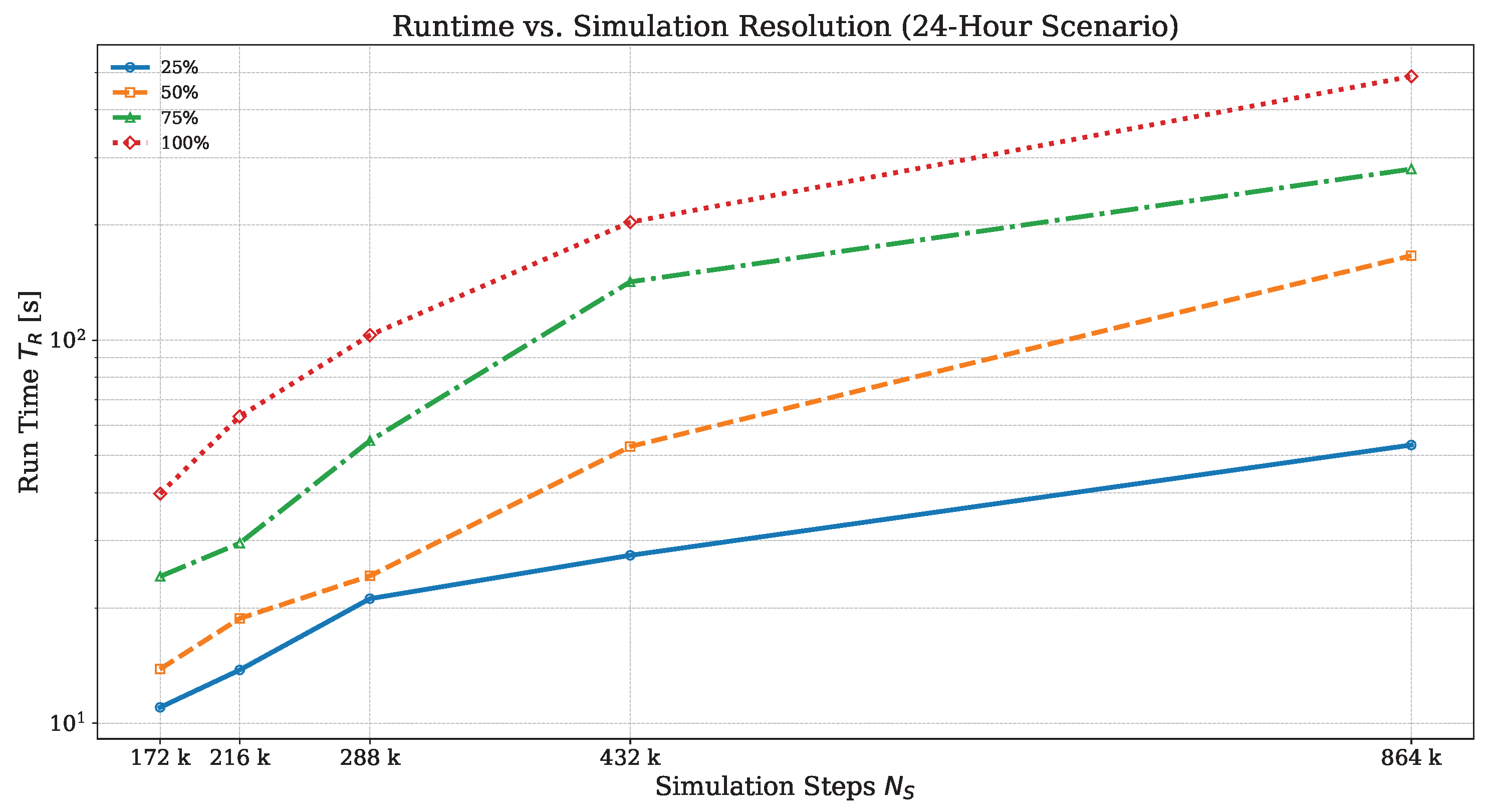
First, we examine with the Bologna scenario how the total runtime $T_R$ increases with the number of simulated time steps $N_S$ (e.g., the total simulated time divided by the simulation step time $T_S$) and the demand level (e.g., the total number of simulated trips). Figure 7 shows that with a five-fold increase in the number of simulation steps $N_S$ (from 172 k to 864 k) the runtime increases proportionally by a factor of $4.8$ at the demand level of $25\%$.

The higher the demand level, the more disproportionately the runtime increases. At a $100\%$ demand level, the runtime increases 12 times when simulation steps are increased only five times. This effect could be explained by the higher number of vehicle transfers and interactions, which means more time is spent on atomic exchangers. However, more profiling is needed to identify the cause of the slowdown.

Next, the performance gains of ParSim, running on the GPU, versus the original SUMO simulation, running on a single core of the CPU, are investigated. Simulations of the 24 h Bologna scenario were repeated under four levels of traffic demand ($25\%$, $50\%$, $75\%$, and $100\%$). In each case, the exact same network, trips, and routes were used by the simulators and the simulation runtimes were recorded. From the runtimes in

Table 5. Simulation runtime comparison between ParSim (on GPU) and SUMO (on CPU) for different demand levels in the Bologna scenario.

Demand Level	Number of Trips	SUMO (CPU)	ParSim (GPU)	Speed Gain
25%	261,279	20,376 s	11.00 s	1852
50%	522,558	49,356 s	13.85 s	3563
75%	783,837	88,128 s	24.18 s	3644
100%	1,045,116	200,916 s	39.76 s	5053

obtained from the Bologna scenario, it is again evident that the simulation times increase with increasing traffic. However, the SUMO simulation seems to be more affected than the ParSim simulation. This may be due to difficulties for SUMO in resolving congestion within the junction. Such artificial congestion can produce queues that can invade and gridlock the entire network. In fact, the average speed of the $100\%$ SUMO simulation decreased to below 1 m/s toward the end of the simulation. SUMO has a teleport procedure (which triggers after a 90 s vehicle standstill) that can temporarily resolve mutual blocking by moving vehicles out of the junction to the next free edge. However, this is often not sufficient and the queues at affected junctions continue to grow. In any case, the performance gains of the GPU-based simulations transcend those of SUMO by factors between 1800 and 5000.

Concerning memory usage, the Bologna testbed exhibits a very compact memory footprint, increasing from only 132 MB at 25% demand to 258 MB at 50%, 404 MB at 75%, and just 503 MB at the full 100% scenario.

The accuracy and reliability of the GPU-based microsimulator have been evaluated by comparing two key indicators obtained from the ParSim and the SUMO simulation: (1) the average waiting time, which is the sum of all times during which the vehicle’s speed drops below 0.1 m/s—this is the way SUMO calculates the waiting time (for example in front of traffic lights)—and (2) the average speed of vehicles during their trips. The results of both indicators are summarized in

Table 6. Comparison of ParSim and SUMO simulation outputs.

Traffic Demand	Avg. Waiting Time [s]		Avg. Speed [m/s]
	ParSim	SUMO	ParSim	SUMO
25%	51.00	61.27	17.30	15.45
50%	76.65	98.53	16.88	14.33
75%	121.74	743.78	15.75	12.88

for the two simulators. The waiting times for ParSim are generally lower and the average speeds higher, especially for higher demand levels. The average travel speeds can be used to quantify the error ParSim is showing with respect to SUMO due to the simplified dynamics at intersections. When comparing these speeds in the two simulators for demand levels where SUMO does not show deadlock phenomena (e.g., the 25% and 50% scenarios), the relative error of ParSim is between 11% and 15%, respectively.

The $100\%$ demand level has not been evaluated, as the SUMO simulation showed excessive congestion due to artificial deadlocks at intersections. Also, the $75\%$ demand level resulted in heavy congestion and gridlock, which is why the SUMO waiting times are considerably higher than those of ParSim for this scenario. ParSim has no gridlock situation, but it can create artificial slow-downs in a situation where the vehicle speed is suddenly set to zero because the successive edge is momentarily occupied. This means that both simulators may show unrealistic behavior but that this behavior occurs in different situations. With SUMO, deadlocks happen at complex and congested intersections, while with ParSim, slow-down effects are more serious if vehicles run at higher speeds and occur more frequently at high vehicle densities.

In order to get a clearer picture of the simulated traffic volumes, we have recorded the number of vehicles entering each edge for ParSim and SUMO. We show only results for the 25% and 50% demand level, as the SUMO starts to show gridlock phenomena for the 75% demand level that is increased even further in the 100% scenario.

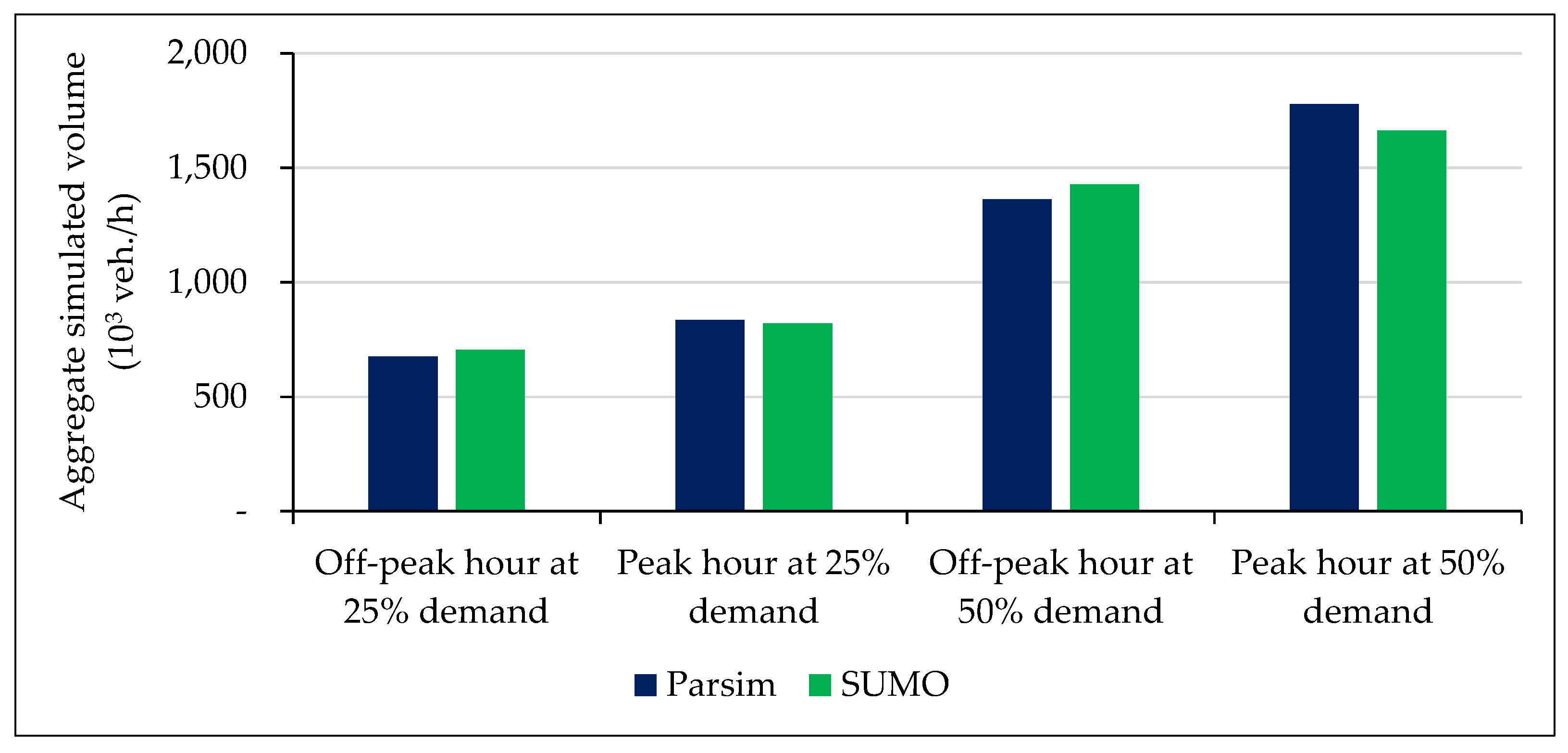
The total traffic volumes (the sum of vehicles entered in all edges) for off-peak and successive peak periods are shown in Figure 8. ParSim and SUMO generated comparable aggregate traffic volumes across all scenarios. At both the 25% and 50% travel demand levels, ParSim estimated lower volumes during the off-peak hour (676.07 vs. 704.30 × ${10}^3$ veh/h at 25% demand and 1362.44 vs. 1427.02 × ${10}^3$ veh/h at 50% demand) and slightly higher volumes during the peak hour than SUMO (836.04 vs. 820.46 × ${10}^3$ veh/h at 25% demand and 1778.91 vs. 1662.64 × ${10}^3$ veh/h at 50% demand). Note that trips have exactly the same start time and the same routes for both simulators. The difference in flows during a certain time window is because the speed and number of crossed edges of an individual vehicle differs in the two simulators due to interactions with other vehicles and traffic lights.

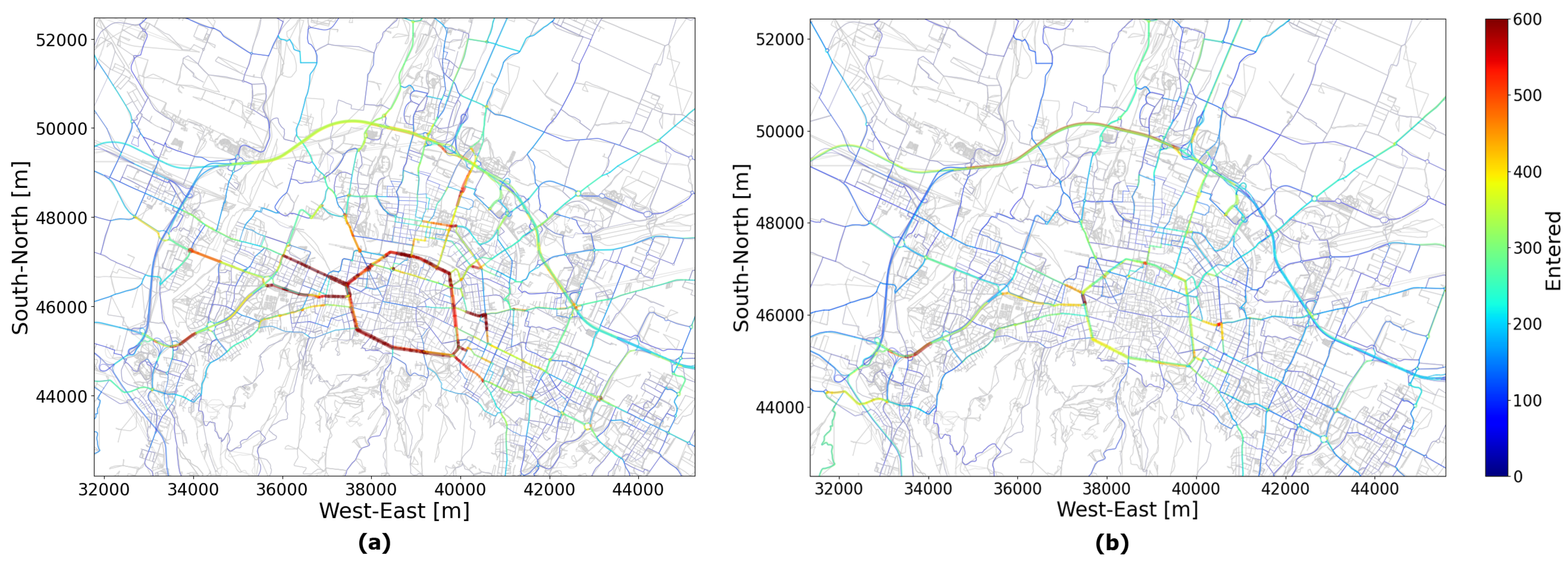
To better visualize the spatial distribution, the simulated edge flows are shown for the peak-hour scenario with $50\%$ travel demand. It can be observed in Figure 9 that edges with high vehicle flows are fairly similar in both ParSim and SUMO: higher traffic volumes are predominantly located along the inner ring road, the radial roads to/from the city center, and the outer ring road. In more detail, the volumes simulated by ParSim are slightly higher than those in SUMO for this scenario (Figure 8), as indicated by the greater presence of red areas with flows reaching up to 500–600 vehicles per hour.

Pearson correlation coefficients (r) and mean absolute errors (MAEs) of edge-level traffic volumes simulated by ParSim and SUMO are compared during peak and off-peak hours under the $25\%$ and $50\%$ demand scenarios, as shown in

Table 7. Pearson’s correlation coefficients (r) and MAEs between ParSim and SUMO simulations.

Indicators	25% Travel Demand		50% Travel Demand
	Off-Peak Hour	Peak Hour	Off-Peak Hour	Peak Hour
Correlation Coefficient (r)	0.87 **	0.88 **	0.89 **	0.90 **
Mean Absolute Errors (MAE)	12.95	14.11	22.26	25.44

Note: ** Correlation is significant at the 0.01 level.

. The results demonstrate positive ($0<r<1$) and strong correlations ($r>0.8$) [34] between the two simulation outputs.

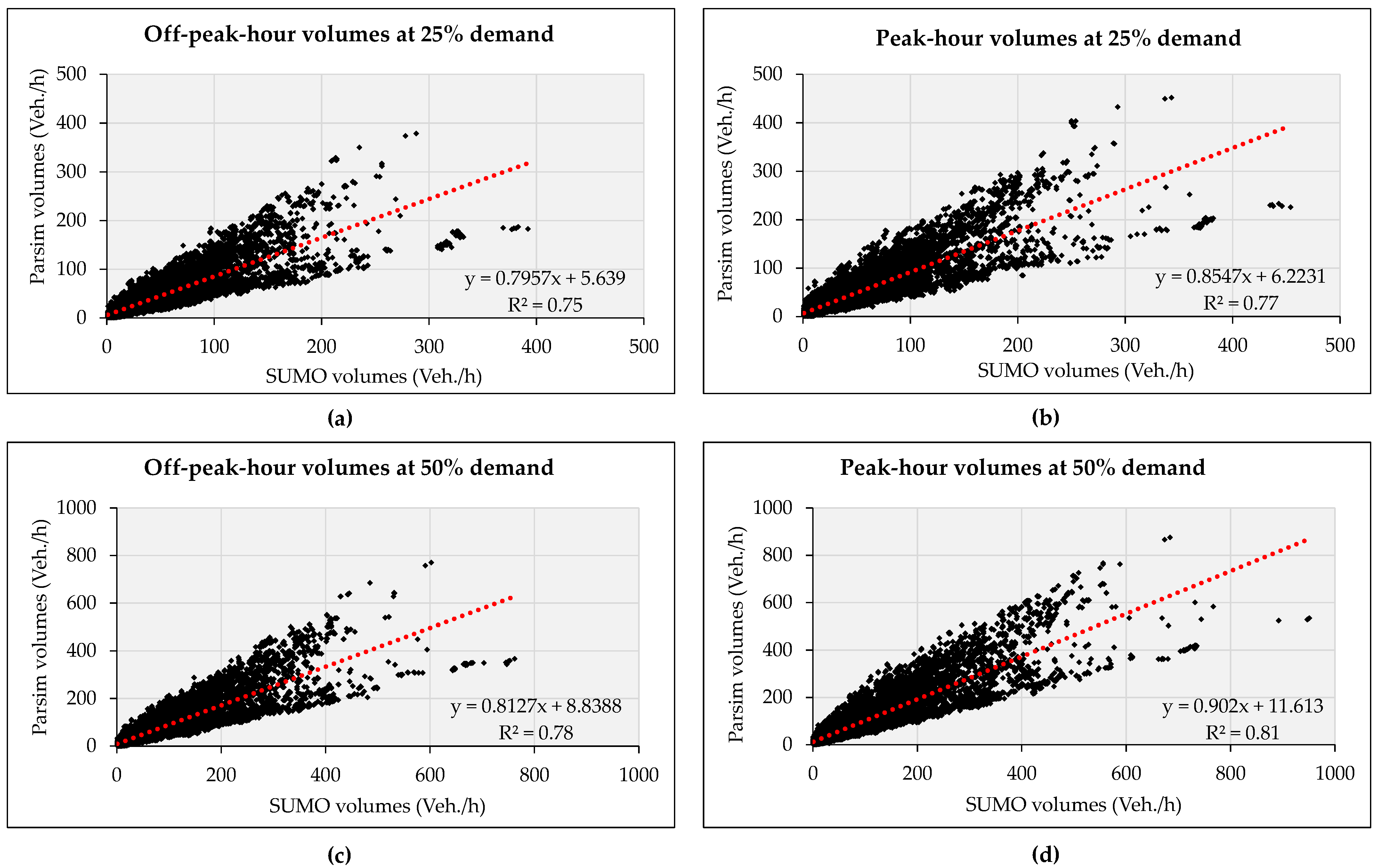
In addition, we also performed a regression analysis between the flows generated by ParSim and SUMO. Figure 10 shows the flows from both simulators for each edge as a dot; slopes and $R^2$ values are also reported. The ParSim simulation results closely matched those of SUMO, especially during peak hours at the 50% travel demand, with a slope of $0.902$ and $R^2$ of $0.81$, which are within acceptable thresholds according to [35].

3.3. Assessment with S.F. Bay Area Scenario

The full 24 h scenario of the S.F. Bay Area with 18 million trips and a rush hour scenario from 7:00 to 9:00 with 3 million trips were used to compare the ParSim simulator presented in this work with the LPSim parallel microsimlator implementation previously developed in [18]. The ParSim simulator completed the 24 h scenario in 1534.68 s or 25.58 min on a single GPU with 8 GB of memory, see

Table 8. Simulation speed and memory usage comparison between ParSim and LPSim.

Scenario	Runtime [s]		Memory Footprint [GB]
	ParSim	LPSim	ParSim	LPSim *
24 h, 18 M trips	1534.68	-	5.07	≈160 **
Rush hour, 3 M trips	21.73	144 ***	0.826	≈40

* These are essentially upper limits, because estimate is based on the number of GPUs in use. ** Corresponding to eight NVIDIA A100 GPUs with 40 GB of memory each. *** LPSim running on a single NVIDIA A100 GPU with 40 GB of memory; no communication between GPUs take place.

. The same scenario was simulated with LPSim using 4× Nvidia A100 graphic cards with 40 GB of memory each. Comparing ParSim with LPSim, it can be concluded that ParSim finished the rush hour 7 times faster while occupying a much less memory on the GPU. These two values are related, as communication between multiple GPUs will slow down the overall simulation process.

4. Discussion

4.1. Main Results

The main results are that ParSim, through its parallelization, is approximately 3000 times faster than a similar SUMO simulation on a single-core CPU. Note that the SUMO simulation tends to show artificial gridlock at large intersections and high traffic flows due to the complex algorithms that resolve conflicts between interacting vehicles. In contrast, ParSim does not have conflicts within the intersection, as vehicles move to the next edge as soon as enough room becomes available. This means that ParSim should not show artificial gridlocks. On the other hand, the simplified intersection handling by ParSim may not only neglect turning delays but also, in the absence of conflicts within junctions, tend to overestimate the throughput in intersections.

The 1 million trips of the 24 h Bologna scenario could be finished in just 41 s, while it took 26 min for the completion of the larger 24 h, 18-million-trip Bay Area scenario. The simulator seems to be seven times faster than LPSim running on a similar scenario, while also occupying less memory on the GPU. However, it should be acknowledged that LPSim has a more detailed lane-change model that allows mandatory lane maneuvers and ParSim did not perform traffic-light operations for this specific scenario. So, the higher speed of ParSim could be partially explained by the simpler simulation processes. In any case, execution times can only be reliably compared by simulating exactly the same network and the same trip patterns.

The simulation results of ParSim were validated by comparing the average waiting times and average speeds with the output of the established SUMO microsimulator. The average travel speeds of ParSim vehicles were approximately 10% higher compared to the average speed determined by SUMO, presumably due to the simpler intersection model of ParSim. In addition, ParSim has the possibility of visual verification and debugging through the GUI capabilities of HybridPy. The visualization turned out to be crucial for code writing and debugging. It can also be helpful for network planning tasks. In addition, the hourly edge flows of ParSim and SUMO have been plotted on a map for comparison. Flows were proportional, but with a distribution around the unit line.

The advantages of the presented simulator are based on multiple design decisions.

• The network and vehicle model have been implemented so that the occupied memory on the GPU is minimized. We have shown that even large-scale simulations, like the one for the San Francisco Bay Area with 8 million inhabitants can fit on a medium-grade GPU with 8 GB of RAM. The fact that all processes take place on a single GPU constitutes a speed advantage over a solution with multiple GPUs, where communications take place; communication can delay processes or bandwidth limitations between the GPUs can become a bottleneck [18].
• The entire simulator has been implemented on a single monolithic kernel, which saves time-losses when swapping kernels on the GPU.
• The implementation of a single kernel introduced some complexity because we had to ensure that the threads during a simulation step are synchronized and that processes are executed in a certain sequential order. Different synchronization techniques, such as atomic exchangers or memory fences, have been used to accomplish this.

4.2. New Applications for Microsimulations

It appears obvious that with the shortened simulation times, microsimulation models can now be employed in a series of applications where they had been too slow in the past. In addition, the ParSim simulator can run on ordinary gaming computers; no expensive hardware is necessary. Potential applications for parallelized microsimulators like ParSim include

• Microsimulations as the main assignment method for activity/plan generation as part of agent-based demand models where traffic assignment is in a loop and needs to be repeated many times. This application may facilitate the creation of larger mobility digital twins of entire cities.
• Training AI agents, such as reinforcement learning or deep RL models, where millions of simulation episodes are needed to converge and slow microsimulations have hindered their usage in the past [11,36].
• Traffic optimization studies, where the system evaluates control strategies, route planning, or congestion mitigation across hundreds of randomized or adaptive scenarios.
• Short-term traffic predictions based on real-time flow measurements [37].
• Crisis response simulation, enabling the fast forecasting of network behavior under incidents or disruptions and supporting real-time decision making. SUMO has already been used in this field [38]; an overview of the current tools and limitations is summarized by Anne-Marie Barthe-Delanoë et al. [39].

4.3. Limitations

The current version of the ParSim simulator lacks useful functionalities that would make the microsimulation model more realistic. One issue is the simplified lane-change model, which does not even allow mandatory lane changes; this may distort the queue length at the lane level. For example, queue formation on the left lane if many vehicles intend to turn left.

ParSim’s simplified lane model also affects the accuracy of the dynamics within the intersection in three different ways. (1) In dense traffic, conflicting vehicle trajectories within intersections are not “seen” by approaching vehicles; therefore, speed adjustments before and within the intersection do not take place. (2) Approaching vehicles do not always complete their speed adjustments before the intersection. This is why a vehicle might come to an abrupt stop when it sees the next edge occupied at the moment it wants to proceed, which in turn causes decelerations upstream. (3) The traffic light can only act on the entire edge but not on single lanes, as lane-to-lane connections are not modeled. The missing conflict modeling at intersections and the simplified traffic lights tend to reduce travel time, while the limited look-ahead capability increases travel times. The results show that the overall effect on travel time is in the range of 11% to 15% compared to the SUMO simulator, where all these effects are modeled. In addition, the results show that the hourly edge flows observed for ParSim are in acceptable correlation with those observed with SUMO.

4.4. Future Developments

A more accurate lane model is certainly a valid feature to implement; the challenge is, of course, not to significantly compromise the simulation speed. One useful extension would be to enable re-routing during the simulation. This feature would allow for more realistic traffic assignments as well as ride-sharing and ride-hailing transport services.

Currently, there is also a lack of flexibility when it comes to producing different kinds of output from the simulation. Such generation of output data needs to be designed carefully—data aggregation or pre-processing should neither significantly reduce simulation speed nor occupy large amounts of memory.

Our simulation design is not limited to a certain GPU type and can easily be ported to more advanced chips with a higher number of CUDA cores—this would immediately result in a higher simulation speed. We also expect notably better performance on GPUs with higher memory bandwidth and improved scheduling efficiency. A larger vehicle population could be simulated in parallel, without the need to fundamentally alter the code design. For instance, an NVIDIA RTX 5090—with 21,760 CUDA cores—one of the high-end GPUs, has seven times as many cores than the GPU used in the present study.

References

1. Patriksson, M. The Traffic Assignment Problem: Models and Methods; Dover Publications, Inc.: Mineola, NY, USA, 2015. [Google Scholar]
2. Lee, K.S.; Eom, J.K.; Moon, D.S. Applications of TRANSIMS in Transportation: A Literature Review. Procedia Comput. Sci. 2014, 32, 769–773. [Google Scholar] [CrossRef]
3. Krajzewicz, D.; Erdmann, J.; Behrisch, M.; Bieker, L. Recent Development and Applications of SUMO—Simulation of Urban MObility. Int. J. Adv. Syst. Meas. 2012, 5, 128–138. [Google Scholar]
4. Koch, L.; Buse, D.S.; Wegener, M.; Schoenberg, S.; Badalian, K.; Dressler, F.; Andert, J. Accurate physics-based modeling of electric vehicle energy consumption in the SUMO traffic microsimulator. In Proceedings of the 2021 IEEE International Intelligent Transportation Systems Conference (ITSC), Indianapolis, IN, USA, 19–22 September 2021; pp. 1650–1657. [Google Scholar] [CrossRef]
5. Fellendorf, M.; Vortisch, P. Microscopic traffic flow simulator VISSIM. In Fundamentals of Traffic Simulation; Springer: New York, NY, USA, 2011. [Google Scholar] [CrossRef]
6. Anya, A.; Rouphail, N.; Frey, H.; Schroeder, B. Application of AIMSUN Microsimulation Model to Estimate Emissions on Signalized Arterial Corridors. Transp. Res. Rec. J. Transp. Res. Board 2014, 2428, 75–86. [Google Scholar] [CrossRef]
7. Liu, R. The DRACULA Dynamic Network Microsimulation Model. In Simulation Approaches in Transportation Analysis; Springer: Boston, MA, USA, 2005; Volume 31, pp. 23–56. [Google Scholar] [CrossRef]
8. Schweizer, J.; Schuhmann, F.; Poliziani, C. hybridPy: The Simulation Suite for Mesoscopic and Microscopic Traffic Simulations. SUMO Conf. Proc. 2024, 5, 39–55. [Google Scholar] [CrossRef]
9. Bowman, J.; Ben-Akiva, M. Activity-based disaggregate travel demand model system with activity schedules. Transp. Res. Part A Policy Pract. 2001, 35, 1–28. [Google Scholar] [CrossRef]
10. Behrisch, M.; Krajzewicz, D.; Flötteröd, Y.P. Comparing performance and quality of traffic assignment techniques for microscopic road traffic simulations. In Proceedings of the DTA2008 International Symposium on Dynamic Traffic Assignment, Leuven, Belgium, 29–31 July 2010; Available online: https://infoscience.epfl.ch/entities/publication/83e8d233-27fd-4b0b-94b7-1548be645f2f (accessed on 20 May 2025).
11. Zhang, H.; Feng, S.; Liu, C.; Ding, Y.; Zhu, Y.; Zhou, Z.; Zhang, W.; Yu, Y.; Jin, H.; Li, Z. CityFlow: A Multi-Agent Reinforcement Learning Environment for Large Scale City Traffic Scenario. In Proceedings of the World Wide Web Conference, San Francisco, CA, USA, 13–17 May 2019; pp. 3620–3624. [Google Scholar] [CrossRef]
12. Auld, J.; Hope, M.; Ley, H.; Sokolov, V.; Xu, B.; Zhang, K. POLARIS: Agent-based modeling framework development and implementation for integrated travel demand and network and operations simulations. Transp. Res. Part C Emerg. Technol. 2016, 64, 101–116. [Google Scholar] [CrossRef]
13. Meister, K.; Balmer, M.; Ciari, F.; Horni, A.; Rieser, M.; Waraich, R.; Axhausen, K. Large-Scale Agent-Based Travel Demand Optimization Applied to Switzerland, Including Mode Choice; Technical Report; ETH Zurich: Zurich, Switzerland, 2010. [Google Scholar] [CrossRef]
14. Spurlock, C.A.; Bouzaghrane, M.A.; Brooker, A.; Caicedo, J.; Gonder, J.; Holden, J.; Jeong, K.; Jin, L.; Laarabi, H.; Needell, Z.; et al. Behavior, Energy, Autonomy & Mobility Comprehensive Regional Evaluator: Overview, Calibration and Validation Summary of an Agent-Based Integrated Regional Transportation Modeling Workflow; Technical Report; LBL Berkeley: Berkeley, CA, USA, 2024. Available online: https://eta-publications.lbl.gov/publications/behavior-energy-autonomy-mobility (accessed on 1 January 2020).
15. DLR. SUMO User Documentation: Duarouter. Available online: https://sumo.dlr.de/docs/duarouter.html (accessed on 1 May 2025).
16. Yedavalli, P.; Kumar, K.; Waddell, P. Microsimulation Analysis for Network Traffic Assignment (MANTA) at Metropolitan-Scale for Agile Transportation Planning. arXiv 2021, arXiv:2007.03614. [Google Scholar] [CrossRef]
17. Waddell, P. SimUAM: A Comprehensive Microsimulation Toolchain to Evaluate the Impact of Urban Air Mobility in Metropolitan Areas. RePEc Res. Pap. Econ. 2021. Available online: https://escholarship.org/uc/item/5709d8vr (accessed on 20 May 2025).
18. Jiang, X.; Sengupta, R.; Demmel, J.; Williams, S. Large scale multi-GPU based parallel traffic simulation for accelerated traffic assignment and propagation. Transp. Res. Part C Emerg. Technol. 2024, 169, 104873. [Google Scholar] [CrossRef]
19. Treiber, M.; Hennecke, A.; Helbing, D. Congested traffic states in empirical observations and microscopic simulations. Phys. Rev. E 2000, 62, 1805. [Google Scholar] [CrossRef] [PubMed]
20. Balmer, M.; Axhausen, K.; Nagel, K. Agent-Based Demand-Modeling Framework for Large-Scale Microsimulations. Transp. Res. Rec. 2006, 1985, 125–134. [Google Scholar] [CrossRef]
21. Maciejewski, M.; Nagel, K. Towards Multi-Agent Simulation of the Dynamic Vehicle Routing Problem in MATSim. In Parallel Processing and Applied Mathematics, Proceedings of the Parallel Processing and Applied Mathematics, Torun, Poland, 11–14 September 2011; Wyrzykowski, R., Dongarra, J., Karczewski, K., Wasniewski, J., Eds.; Springer: Berlin/Heidelberg, Germany, 2012; pp. 551–560. [Google Scholar]
22. Lowndes, V.; Bird, A.; Berry, S. Introduction to Cellular Automata in Simulation. In Guide to Computational Modelling for Decision Processes: Theory, Algorithms, Techniques and Applications; Springer International Publishing: Cham, Switzerland, 2017; pp. 55–73. [Google Scholar] [CrossRef]
23. DLR. SUMO User Documentation: Why Vehicles Are Teleporting. Available online: https://sumo.dlr.de/docs/Simulation/Why_Vehicles_are_teleporting.html (accessed on 6 June 2025).
24. Klöckner, A.; Pinto, N.; Lee, Y.; Catanzaro, B.; Ivanov, P.; Fasih, A. PyCUDA and PyOpenCL: A Scripting-Based Approach to GPU Run-Time Code Generation. Parallel Comput. 2012, 38, 157–174. [Google Scholar] [CrossRef]
25. Egielski, I.J.; Huang, J.; Zhang, E.Z. Massive atomics for massive parallelism on GPUs. In Proceedings of the 2014 International Symposium on Memory Management, ISMM ’14, Edinburgh, UK, 12 June 2014; pp. 93–103. [Google Scholar] [CrossRef]
26. Zhang, L.; Wahib, M.; Matsuoka, S. Understanding the overheads of launching CUDA kernels. In Proceedings of the ICPP19, Kyoto, Japan, 5–8 August 2019; pp. 5–8. [Google Scholar]
27. NVIDIA Corporation. CUDA C++ Programming Guide, Version 12.9; NVIDIA Corporation: Santa Clara, CA, USA, 2025. Available online: https://docs.nvidia.com/cuda/archive/12.3.0/ (accessed on 6 June 2025).
28. Dang, H.V.; Schmidt, B. CUDA-enabled Sparse Matrix–Vector Multiplication on GPUs using atomic operations. Parallel Comput. 2013, 39, 737–750. [Google Scholar] [CrossRef]
29. Feng, W.C.; Xiao, S. To GPU synchronize or not GPU synchronize? In Proceedings of the 2010 IEEE International Symposium on Circuits and Systems (ISCAS), Paris, France, 30 May–2 June 2010; pp. 3801–3804. [Google Scholar] [CrossRef]
30. Tuomanen, B. Hands-On GPU Programming with Python and CUDA: Explore High-Performance Parallel Computing with CUDA; Packt Publishing Ltd.: Birmingham, UK, 2018. [Google Scholar]
31. Foundation, O. OpenStreetMap. Available online: http://www.openstreetmap.org/ (accessed on 6 June 2025).
32. Nguyen, N.A.; Poliziani, C.; Schweizer, J.; Rupi, F.; Vivaldo, V. Towards a Daily Agent-Based Transport System Model for Microscopic Simulation, Based on Peak Hour O-D Matrices. In ICCSA 2024, Proceedings of the Computational Science and Its Applications—ICCSA 2024, Hanoi, Vietnam, 1–4 July 2014; Gervasi, O., Beniamino, M., Garau, C., Taniar, D., Rocha, C., Ana, M.A., Lago, F., Noelia, M., Eds.; Springer: Cham, Switzerland, 2024; pp. 331–345. [Google Scholar]
33. Schweizer, J.; Poliziani, C.; Rupi, F.; Morgano, D.; Magi, M. Building a large-scale micro-simulation transport scenario using big data. ISPRS Int. J. Geo-Inf. 2021, 10, 165. [Google Scholar] [CrossRef]
34. Profillidis, V.; Botzoris, G. Chapter 5—Statistical Methods for Transport Demand Modeling. In Modeling of Transport Demand; Profillidis, V., Botzoris, G., Eds.; Elsevier: Amsterdam, The Netherlands, 2019; pp. 163–224. [Google Scholar] [CrossRef]
35. Cascetta, E. Transportation Systems Engineering: Theory and Methods; Kluwer Academic Publisher: Boston, MA, USA; Dordrecht, The Netherlands; London, UK, 2001. [Google Scholar]
36. Tang, Y.; Qu, A.; Jiang, X.; Mo, B.; Cao, S.; Rodriguez, J.; Koutsopoulos, H.N.; Wu, C.; Zhao, J. Robust Reinforcement Learning Strategies with Evolving Curriculum for Efficient Bus Operations in Smart Cities. Smart Cities 2024, 7, 3658–3677. [Google Scholar] [CrossRef]
37. Perera, T.; Gamage, C.N.; Prakash, A.; Srikanthan, T. A Simulation Framework for a Real-Time Demand Responsive Public Transit System. In Proceedings of the 2018 21st International Conference on Intelligent Transportation Systems (ITSC), Maui, HI, USA, 4–7 November 2018; pp. 608–613. [Google Scholar] [CrossRef]
38. Li, H.; Zhao, D.; Zhu, X.; Fan, W.; Wang, W. Research on SUMO-Based Emergency Response Management Team Model. In Proceedings of the 2007 International Conference on Wireless Communications, Networking and Mobile Computing, Shanghai, China, 21–25 September 2007; pp. 4606–4609. [Google Scholar] [CrossRef]
39. Barthe-Delanoë, A.M.; Truptil, S.; Benaben, F. Towards a taxonomy of crisis management simulation tools. In Proceedings of the ISCRAM 2015 Conference, Kristiansand, Norway, 24–27 May 2015; p. 7. Available online: https://imt-mines-albi.hal.science/hal-01697535 (accessed on 6 June 2025).
Figure 1. Scheme with the basic elements and quantities of the parallelized simulation model. (a) Network representation: Each edge is subdivided in one or several segments in the longitudinal direction and lanes in the transversal direction. Note that the follower vehicle 2 is able to look ahead and recognize the distance to vehicle 1. (b) The quantities necessary to calculate the vehicle acceleration using the IDM vehicle following model, as explained in Section 2.2.
Applsci 15 06960 g001
Figure 2. Synchronization procedure of CPU and GPU in ParSim.
Applsci 15 06960 g002
Figure 3. Scheme showing how traffic-light logic (TLL) threads and vehicle threads are organized on the GPU.
Applsci 15 06960 g003
Figure 4. Implementation architecture of kernel in ParSim.
Applsci 15 06960 g004
Figure 5. An example of an atomic operation with two vehicles on a two-lane edge approaching a single-lane edge that is occupied by another vehicle.
Applsci 15 06960 g005
Figure 6. Graphical User Interface of HybridPy with data browser (left panel) and interactive network visualization (in blue), foodpath (in green) and reserved roads (in purple) and vehicles (in yellow). Below the network are the buttons to operate the ParSim. Note that the vehicle queues waiting at a traffic light and two bicycles running on the red bikepath.
Applsci 15 06960 g006
Figure 7. Increase of simulation runtime T R with an increasing number of iterations and demand levels in the Bologna scenario. Note the logarithmic scale of the simulation runtime.
Applsci 15 06960 g007
Figure 8. Aggregate traffic volumes from ParSim and SUMO across the simulation area under different travel demand thresholds.
Applsci 15 06960 g008
Figure 9. Spatial distribution of simulated traffic volumes from ParSim (a) and SUMO (b).
Applsci 15 06960 g009
Figure 10. The regression diagrams present the comparison of the simulated traffic volumes between ParSim and SUMO over different demand thresholds and time periods: the 25% travel demand in the off-peak (a) and peak hours (b) and the 50% travel demand in the off-peak (c) and peak hours (d). Red dashed lines represent the linear regression y ( x ) , see labels in each graph.
Applsci 15 06960 g010