Micro-Location Temperature Prediction Leveraging Deep Learning Approaches

Abstract

Nowadays, technological progress has promoted the integration of artificial intelligence into modern human lives rapidly. On the other hand, extreme weather events in recent years have started to influence human well-being. As a result, these events have been addressed by artificial intelligence methods more and more frequently. In line with this, the paper focuses on searching for predicting the air temperature in a particular Slovenian micro-location by using a weather prediction model Maximus based on a long-short term memory neural network learned by the long-term, lower-resolution dataset CERRA. During this huge experimental study, the Maximus prediction model was tested with the ICON-D2 general-purpose weather prediction model and validated with real data from the mobile weather station positioned at a specific micro-location. The weather station employs Internet of Things sensors for measuring temperature, humidity, wind speed and direction, and rain, while it is powered by solar cells. The results of comparing the Maximus proposed prediction model for predicting the air temperature in micro-locations with the general-purpose weather prediction model ICON-D2 has encouraged the authors to continue searching for an air temperature prediction model at the micro-location in the future.

1. Introduction

Generally, air temperature forecasts have improved enormously in recent years, but there are still large variations at micro-locations where the differences in air temperatures can be huge. To build more accurate forecast models for such micro-locations, it is necessary to have professional meteorological stations, measurements from drones, satellites, weather balloons and to update the weather models as often as possible with new data, as this is the only way to detect sudden changes in the weather at a particular micro-location and its surrounding area. Unfortunately, there are currently too few meteorological stations to improve the built weather model for air temperature forecasts at each micro-location. This prediction can only be performed at those micro-locations where we have good-quality and frequent meteorological data obtained from professional meteorological stations.

The forecasting of various parameters at micro-locations or specific limited geographical areas has been explored in several research studies. For instance, Kim et al. [1] addressed the challenge of predicting fine dust levels at specific micro-locations where observatories are absent, relying on datasets collected from meteorological stations. Their study proposed an innovative strategy that incorporates micro-location data, specifically latitude and longitude, to enhance prediction accuracy. Similarly, Agarwal et al. [2] introduced a novel approach that combines hyperlocal weather prediction with anomaly detection using the Internet of Things (IoT) sensor networks and advanced Machine Learning (ML) techniques. IoT sensors are hardware components capable of bridging the physical and digital worlds. They are seamlessly connected to the Internet, enabling automation, predictive maintenance, and data-driven insights. These sensors represent building blocks for establishing modern concepts, like Industry 5.0 [3] and Agriculture 5.0 [4]. By leveraging data from multiple spatially distributed but relatively close locations, their method produces high-resolution weather models capable of predicting short-term localized conditions such as temperature, pressure, and humidity. An interesting perspective is presented by Deznabi et al. [5], who developed a transformative model employing a mechanism to extrapolate location embeddings from data-rich regions to target locations with limited training data. This approach enables accurate forecasting for previously untrained areas, demonstrating the potential of advanced spatial modeling techniques to address data scarcity. Apart from the work of Hochreiter and Schmidhuber [6], we distinguish between short-term quality and reliable weather data obtained from weather stations, as well as long-term dependencies inherited within sensor networks [7,8].

Nowadays, predicting air temperature is typically based on weather datasets that vary between each other in the spacial resolution of weather data referring to a specific region. Indeed, we distinguish between lower- and higher-resolution weather datasets, where the former include weather data from relatively large regions (e.g., 5.5 km of spacial resolution), while the latter are more detailed (e.g., less than 2.5 km of spacial resolution). On the other hand, the lower-resolution datasets include long-term historical weather data (i.e., in more than a 40 year period) sampled at one hour intervals, while the higher-resolution datasets incorporate short-term history weather data sampled in the last two years at three hour intervals. In line with this, a micro-location refers to the highest resolution dataset including current weather data of the specific location (i.e., 0 km of spacial resolution) that needs to be obtained from a mobile weather station. Let us mention that micro-meteorological elements, like dew and scintillation in the lower layers of the troposphere, are not included in the study explicitly because they are indirectly already included in the prediction model [9]. Therefore, we need to find the best available model publicly, which would be the best approximation for a specific micro-location. Validation from a real weather station improves the prediction of the weather models that are too general because it can consider the micro-climatic conditions for the specific micro-location in the prediction.

In the case of predicting air temperature at a micro-location, the challenge is even greater, as the terrain can be very rugged and the air temperature can be completely different just a few meters down from our weather station location. Also, a sudden shower or thunderstorm can cool the atmosphere very much above the measurement site, while, a few kilometers away it is completely dry, and there is no sudden change in air temperature. When monitoring sudden weather events with dynamic and turbulent changes of air masses, it is difficult to predict the air temperature, especially, in the north-eastern part of Slovenia due to the arrival of south-westerly winds in anticipation of a change in the weather situation, mostly before the weather worsens, which warms the atmosphere very quickly. However, the areas with less winds can have temperatures more than 10 degrees Celsius lower than windward areas. The differences can be approximately a few hundred meters, and predicting such situations also represents a challenge.

In general, weather forecasting is influenced by a huge number of factors. To add to this, the butterfly effect and a small deviation in the initial forecast conditions can critically change the whole weather situation. Therefore, one of the major challenges is to find such parameters as inputs to the forecast model that are capable of both (1) taking the quality of the measurements from the weather station into account and (2) reducing the error of the forecasting model based on high-resolution datasets [10].

As a matter of fact, we tried to solve the air temperature prediction problem by analyzing different weather situations and observing how well the learned air temperature prediction models reacted to each weather situation. It is assumed that some of these learned prediction models will react better in, e.g., sunny weather, while others will react better in, e.g., a rapid cooling in the middle of the day. This could mean that the classifiers could be used for determining which prediction model could be used for a particular weather situation, but the model selection will be toward the most optimal model that will be the best at identifying general weather patterns for a given situation. Moreover, the metrics with which we evaluate our model must provide some indication of the performance of the learned model in predicting a sequence of air temperature values for the next few hours, but this does not mean that it is capable of predicting all weather situations so well. As a result, we really need to decide very carefully about which learned prediction model to use.

Our proposed prediction model, called Maximus, has the ability to remember short- and long-term details. Therefore, this is ideal for solutions using Machine Learning (ML) methods that are capable of dealing with time-series data, in our case, Long Short-Term Memory (LSTM). Although more suitable state-of-the-art combinations of either convolution neural network (CNNs) [11] and LSTM or models with attention mechanisms also exist, the goal or our study was to show that the prediction of air temperature at the micro-location can be improved by using the optimal LSTM model. The authors of the paper are aware that the prediction could also be improved by using an advanced prediction method, but this subject is left for future work. The advantage of using meteorological knowledge is in choosing those features that contribute the most to the prediction without much further calculation of different combinations of hyper-parameter settings controlling the model’s architecture. The Maximus prediction method was tested for predicting the air temperature at a given Slovenian micro-location. The comprehensive experiments revealed that the proposed prediction model can predict the air temperature for the given micro-location more accurately than other general-purpose weather prediction systems.

The original novelties of the proposed prediction model Maximus can be summarized as follows:

• To build the optimal prediction model based on the lower-resolution CERRA dataset including long-term weather data;
• To find the more optimal characteristics of the used LSTM Neural Network (NN) by indicating those features, their number and types that have the greatest impact on the correct prediction of the air temperature on the micro-location;
• To improve the simulation of the optimal prediction model with weather data obtained from the reference, general-purpose ICON-D2 weather prediction model updated with current weather data from the weather station positioned at micro-location;
• To change the location of the weather station, determining the micro-location exactly, easily with its mobility.

In line with this, we pose the following research question: How can we train a weather classification model to predict air temperature for a given micro-location?

The structure of the remainder of the paper is as follows: In Section 2, the materials and methods used in the study are discussed. Section 3 illustrates the proposed prediction method Maximus. A description of the experiments and obtained results are the subjects of Section 4. The paper concludes with a summarization of the performed work in Section 5, which also outlines potential directions for further work.

2. Material and Methods

The purpose of this section is to review the material and methods used in our study. In line with this, the section focuses on the following issues:

• Weather stations;
• Weather datasets;
• Prediction methods.

The weather station is responsible for monitoring, tracking, and collecting weather data that have arisen at different sensors. These data enable us to build proper weather models for a specific micro-location, and serve as a knowledge database for the prediction methods responsible for predicting the air temperature of a micro-location in the future. All mentioned issues are discussed in more detail in the remainder of this paper.

2.1. Weather Station

Because of their quality and relevance, it is important to use data from the nearest meteorological station that provides the most high-resolution time data possible. At the same time, this station must provide good quality measurements and sensor placements. Both mentioned issues have a decisive influence on the results of the experiment.

The meteorological station is also capable of maintaining a history, inspecting the sensors and validating the data. With daily monitoring of the station’s performance, we can obtain metadata to help us when we detect certain extreme values that may indicate a failure of the station or a particular sensor.

These stations need to be designed as closely as possible according to the World Meteorological Organization (WMO) standards [12], which ensure comparability between other measurement data recorded on different meteorological instruments worldwide. There are two main characteristics of the station, as follows:

• The location;
• The architecture of the meteorological station.

The first characteristic refers to a particular micro-location, while the architecture determines the type and quality of the weather data acquired by the control unit.

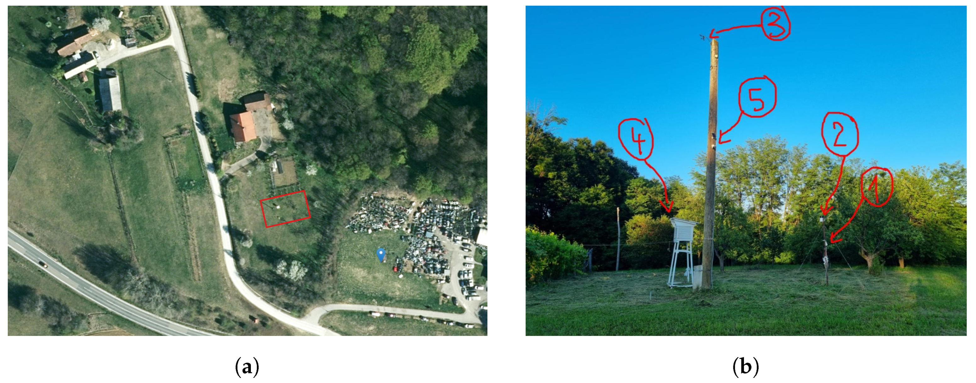
The meteorological station used in our study is located at an altitude of 291 m above sea level. The coordinates of the station are 46,6002° north latitude and 15,8770° east longitude. Thus, the red square in Figure 1a indicates the location of the meteorological station. As seen in the satellite image Figure 1a, our weather station is located in an area with a garden nearby, no buildings, and no forest in a 50 m radius. The terrain is a bit hilly, so the station is on a small hill. For the wind parameter, only the forest blocks the east side; other directions are open.

As the station is located in a small village, there is no urban area within a few kilometers of the station. There is a lot of vegetation around. The location was also carefully chosen, taking into consideration WMO standards. Few trees are located near the station; moreover, there is a clear view, and the effects of the urban area should be minimal.

In Figure 1b, the architecture is described by the position of the sensors with which the meteorological station is equipped. The sensors are either embedded into or connected to the central unit. All the components of the station are designated with numbers surrounded by circles in the figure, denoting the following:

• The central unit with an embedded air pressure sensor and integrated solar panels;
• The rain gauge;
• The anemometer;
• The Stevenson screen containing temperature and relative humidity;
• A webcam that can record the whole setup and presents the real weather situation at the micro-location online.

The mentioned components are discussed in detail in the remainder of the paper.

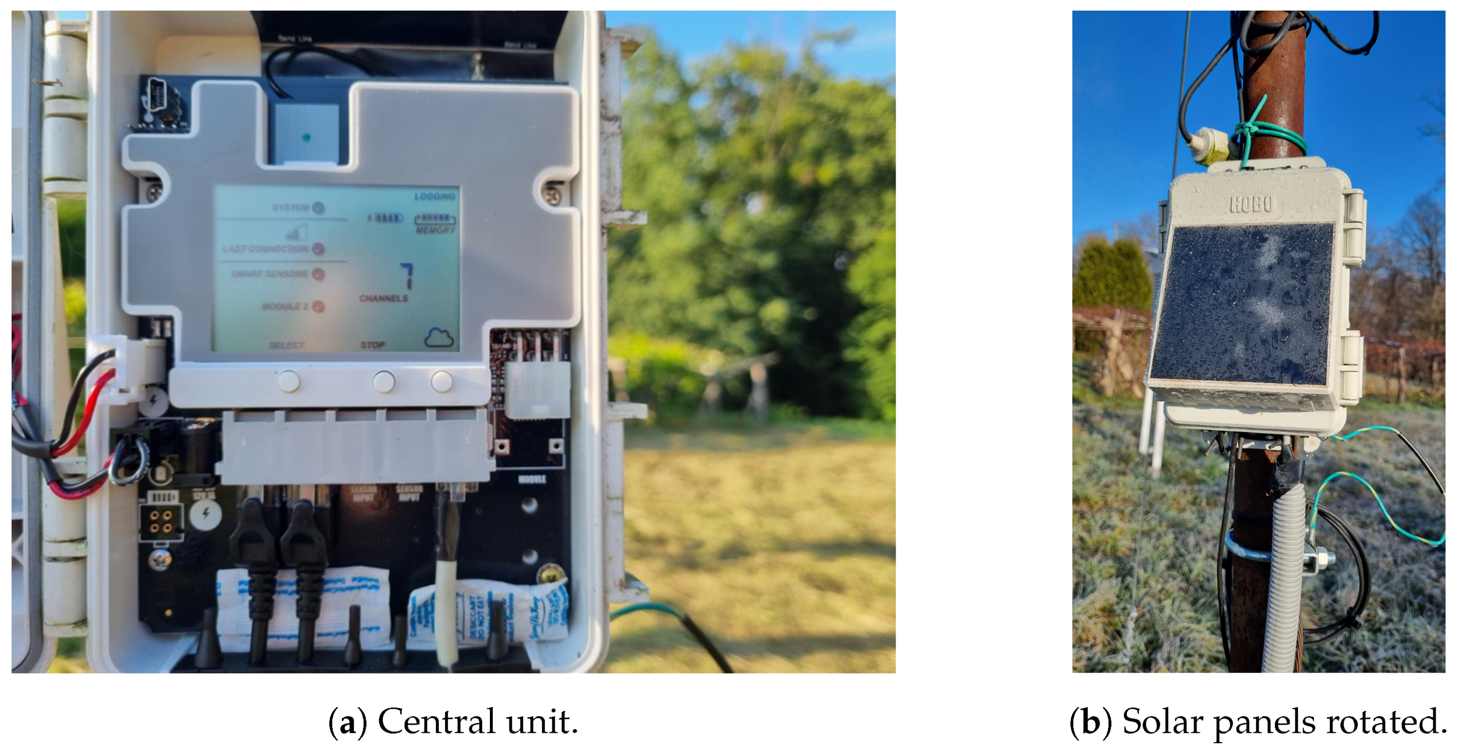
2.1.1. Central Unit, with an Air Pressure Sensor and Solar Panels

All the sensors, except the absolute air pressure sensor and integrated solar panels, are connected to a central unit (Figure 2a). The central unit processes all the signals received over the wire, stores them, and sends them to the cloud via the network at 10 min intervals. The display shows basic information on the strength of the network signal, from the battery and various statuses to the operation of the modules and individual alarms. In the event of a network outage, the control panel stores the data in its memory, and only sends them to the cloud when the network is back up and the connection is working smoothly. The central unit also has the option of lightning protection by connection to a copper wire.

The absolute air pressure sensor is embedded into the central unit. The absolute air pressure represents the actual air pressure in a given space and time. From it, the relative air pressure can be obtained, which is calculated, among other things, by using the altitude data. The accuracy of the sensor is illustrated in Section 2.1.3.

The device has an integrated 1.7 watt solar panel with lithium batteries (Figure 2b). The device operates flexibly in the rural areas, still sending data with a weak cellular network signal. In case of problems connecting to the cloud at a particular time, it stores the data, and sends them all when the connection can be re-established. The battery life, without solar recharging, with hourly connections and 1 min logging, can last several months. The battery’s life extends from 3 to 5 years under temperature conditions from −20 °C to 40 °C. It is possible to use connection intervals as frequent as up to 10 min to send data to the cloud. This frequency is crucial for draining the battery and recharging it via solar panels, as in the winter, because of the fog, it is often the case that we need to set a less frequent connection interval between the device and cloud to ensure healthy operating conditions.

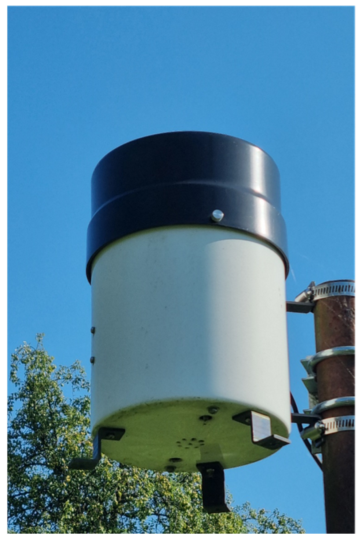
2.1.2. Rain Gauge

It is recommended that the rainfall sensor is placed in a location where there are no obstructions that would prevent rain from falling into the sensor container. Wind is a major problem for the accuracy of the rainfall measurement, because it can simply carry a large proportion of the rainfall past the opening, as it carries the rain at a more oblique angle. This can lead to a large error in the rainfall measurement. However, a heated rain gauge can be used to measure the height of the snow cover, where snowflakes turn into water droplets upon contact with the container. It is also important that the rain gauge is very well fixed and that, in the event of a strong wind, there is no vibration to move the balance in the container and thus contribute to erroneous precipitation measurements. The height of the installation in our case is two meters above the ground, and the sensor is placed on a well-fixed pole with individual additional reinforcements [13] (Figure 3). The accuracy of the sensor can be seen in

Table 1. Characteristics of rainfall measurements with tipping points [14].

Measuring Characteristics	Values
Manufacturer	HOBO rain gauge
Model	RG3
Resolution	$0.10 °$C at $25 °$C ($0.18 °$F at $77 °$F)
Calibration	Requires annual calibration
Measurement range	$-20 °$C to $70 °$C ($-4 °$F to $158 °$F)
Accuracy	$\pm 0.47 °$C at $25 °$C ($\pm 0.85 °$F at $77 °$F)
Max. 4000 tipping points/logging interval	1% error up to 127 mm/h

.

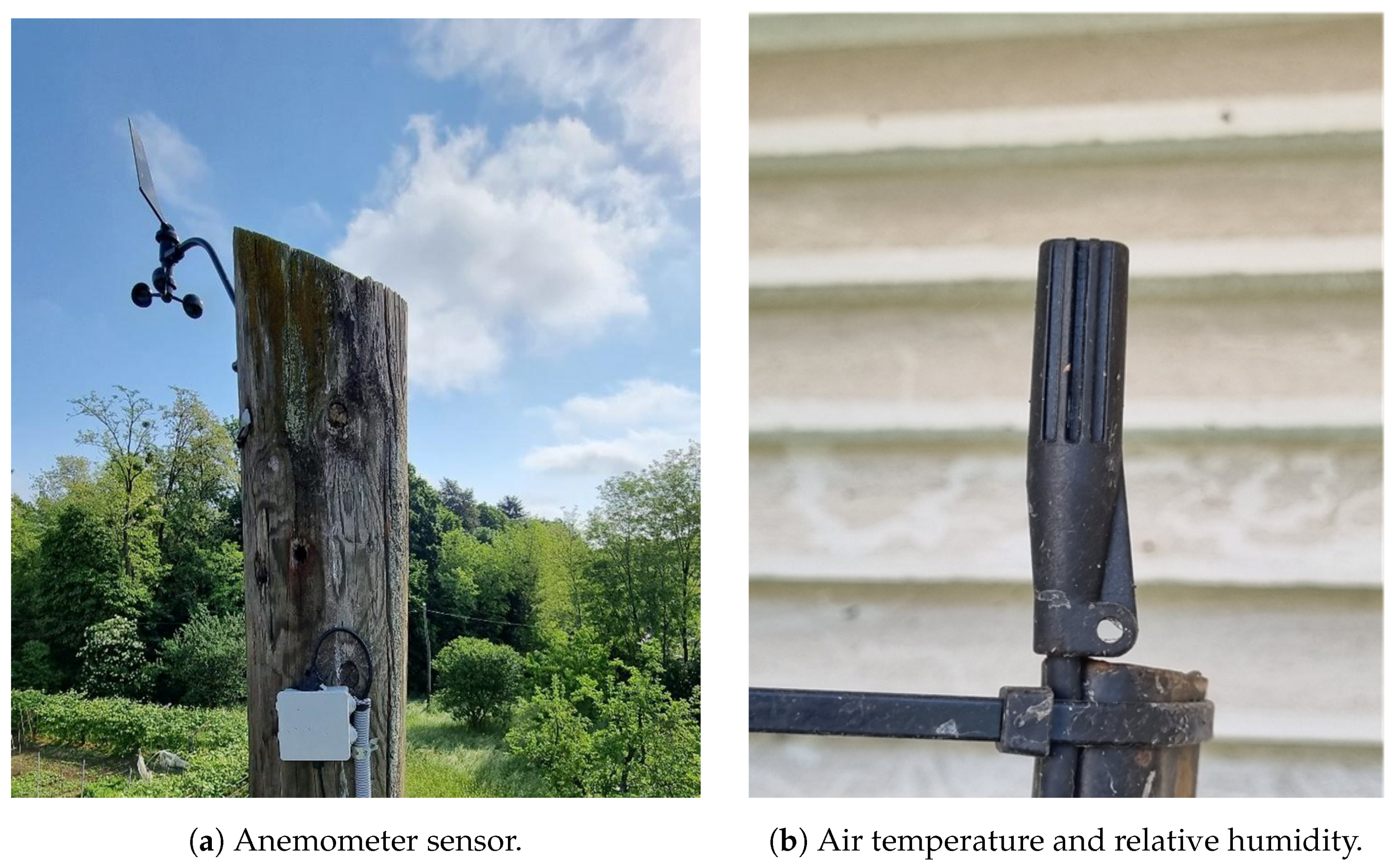
2.1.3. Anemometer

The wind sensor has three channels for wind speed, gusts, and wind direction. Obstacles also have a significant effect on wind measurements, so the height of the sensor should normally be 10 times the height of the obstacle. The standard sensor height is 10 m above the ground. In our case, the wind sensor is placed at a height of approximately 8.6 m above the ground [13] (Figure 4a). Interestingly, the accuracy of the sensor can be seen in

Table 2. Accuracies of the sensors.

(a) Air pressure sensor.		(b) Anemometer.
Measuring Range	Accuracy	Measuring Range	Accuracy
66 kPa to 107 kPa	±0.2 kPa	From 0 to 76 m/s	±1.1 m/s

b.

2.1.4. Temperature and Relative Humidity

The air temperature sensor is usually placed at a height of 2 m from the ground. The sensor requires a good-quality shield against solar radiation. For this purpose, it should be placed in a pre-planned shade (Figure 4b). This shade must have a sufficiently good air permeability to react quickly to temperature changes [13]; the accuracy of the sensor is presented in

Table 3. Accuracies of the temperature sensor.

Measuring Range	Accuracy
−40 °C to 100 °C	±0.2 °C

.

The relative humidity sensor is combined with the air temperature sensor, and is thus placed at the same height and under the same conditions as the air temperature sensor [13] (Figure 4b). The data on the characteristics of the sensor are aggregated in

Table 4. Characteristics of relative humidity sensor [15].

Measuring Characteristics	Values
Measurement range	$-40 °$C to $75 °$C ($-40 °$F to $167 °$F)
Accuracy	$\pm 0.25 °$C from $-40 °$C to $0 °$C ($\pm 0.45 °$F from $-40 °$F to $32 °$F)
Resolution	$0.02 °$C
Operating temperature range	$-40 °$C to $75 °$C ($-40 °$F to $167 °$F)

. The manufacturer calibrated the software. Therefore, we did not apply a special calibration method. Temperature and relative humidity were logged every minute.

2.2. Weather Datasets

The rapidly growing number of weather datasets, as well as continuous improvements in technology and public availability, have enabled scientists to dive into the details of sophisticated weather models and their mathematical and physical background. A more universal approach to this issue has been adopted by the Copernicus Climate Change Service (C3S) society, who provide authoritative information about the past, present and future climate in Europe and the rest of the world. The aim of the society is to produce and deliver Regional ReAnalysis (RRA) weather data for Europe. The reanalysis combines model data with observations, into a complete and consistent dataset using the laws of physics. The Copernicus European Regional Reanalysis (CERRA) datasets provide spatially and temporally consistent historical reconstructions of the meteorological variables in the atmosphere and at the surface. CERRA is the generic name for the following three datasets [16]:

• CERRA: the high-resolution dataset produced at a horizontal resolution of 5.5 km containing atmospheric and surface variables.
• CERRA-EDA: the dataset contains atmospheric and surface variables produced at a horizontal resolution of 11 km by a 10-member ensemble of data assimilation systems.
• CERRA-Land: this dataset contains precipitation and soil variables available at a 5.5 km grid spacing.

These datasets provide reanalysis data on model levels for Europe from 1984 to the present. Indeed, CERRA is the most suitable one for our experimental study, as it contains the surface variables that we need to integrate into our learning procedure. Conceptually, it belongs to the category of lower-resolution datasets.

On the other hand, the German National Weather Agency (ger. Deutscher Wetterdiens, DWD) [17] offers access to many climate data from the Climate Data Center (CDC) [18] for further processing. Moreover, the same agency also offers several Numerical Weather Prediction (NWP) models, like [19]: the global ICOsahedral Nonhydrostatic (ICON), and two regional ICON-EU and ICON-D2. ICON defines the domain that covers the global region including most of the Atlantic Ocean, Greenland, and Europe, extending a little bit to the east and south with a horizontal resolution of 13 km. ICON-EU enables weather prediction in regions inside ICON, which serve as the initial conditions to this “local nest” model with a horizontal resolution of about 7 km. In this way, it covers Europe and extends to a small area in Africa, and also to the east. For the purpose of creating an higher-resolution weather model, ICON-D2 Regional NWP (RNWP) was created, with a horizontal resolution of about 2.2 km, which provides new 48 h forecasts every 3 h [19]. This high-resolution weather dataset is available for Central Europe, including Slovenia [20].

Moreover, the ICON-D2 weather dataset has much better horizontal resolution than its predecessors. The details including land use, a digital elevation model, and other terrestrial data are crucial to capture the local weather circulations, including turbulence and local advection. Convective clouds have much better local precision with more detailed orography, and can simulate precipitation more accurately, including thunderstorms which are very local in nature.

2.3. Prediction Methods

Many different ML and Deep Learning (DL) methods exist for weather prediction. In this study, we focus in particular on a DL method called LSTM [6], which is a type of recurrent neural network (RNN) [21].

Yu et al. [22] described the application of this method based on data acquired from IoT temperature sensors through the main thoroughfares of New York City, America, where the air temperature sensors were placed at a distance of about 150 m. The main point is a prediction of the hourly air temperature for the next day. The LSTM method learns over the data from all measurements and locations to obtain an accurate prediction.

Liang et al. [7] presented a combination of several LSTM-based layers that do not support backward data searching in the model learning process. Consequently, a new version of the LSTM model was implemented which supports both backward and forward data searching, and thus increased the accuracy of the model prediction.

Combining CNN and LSTM gives a better combination and thus better predictions. CNN reduces the dimensionality of the time series data, while LSTM is able to capture the memory of long time periods in the air temperature data. Missing data, data standardization, and interpolation were taken care of during data preparation [8].

A very interesting combination was presented by Suleman and Shridevi [23], which included the attention mechanism, to capture the links between several meteorological parameters for air temperature prediction successfully. This model has the ability to learn from the temporal and spatial features and interactions between the data. When evaluated using different combinations of models, it received the best Mean Squared Error (MSE) and Mean Absolute Error (MAE) metrics among all the other metrics.

The work of Agarwal et al. [2] describes a spatial short-term forecast of unusual weather events or patterns that can be used to warn the population of an impending hazard. Using IoT, a change in anomalies is identified where high-resolution weather models are used. The use of unsupervised learning algorithms is used to find unusual patterns.

As an alternative, solar irradiance prediction using meteorological data in parts of Bangladesh was also used in study by Faisal et al. [13]. Thus, three different NNs were compared: RNN, LSTM, and Gated Recurrent Unit (GRU) [24]. Using meteorological data from the previous day, it was possible to predict solar irradiance for future dates. The best model with respect to the Mean Absolute Percentage Error (MAPE) metric was GRU, with a score of 19.28.

Although LSTM has much better results than traditional statistical methods in predicting the time-series of large amounts of data, the combinations of the LSTM model with other methods, namely LSTM-SAE, work better, as described by Sagheer and Kotb [20]. If we have to process very non-linear data and long time-series, namely with supervised learning, we do not achieve good enough results. Therefore, the use of an unsupervised learning and LSTM-SAE model combination is proposed.

Based on the time-series data, the following combined method to improve the prediction accuracy, called ConvLSTM, was also proposed by Fu et al. [25]. The ConvLSTM combines the CNN and the LSTM model. A stand-alone attention mechanism was implemented for improved temporal resolution and pattern detection. A combined Bi-LSTM method [26], which uses traditional coding and temporal attention learning, has also been presented to work with data involving multiple variables. This yields long time dependence and a hidden correlation between the parameters in the data. The results with regard to the RMSE metric are the best compared to other methods. In the study of Gangopadhyay et al. [27], the attention mechanism was also used to match the most relevant temporal data.

3. Proposed Method Maximus

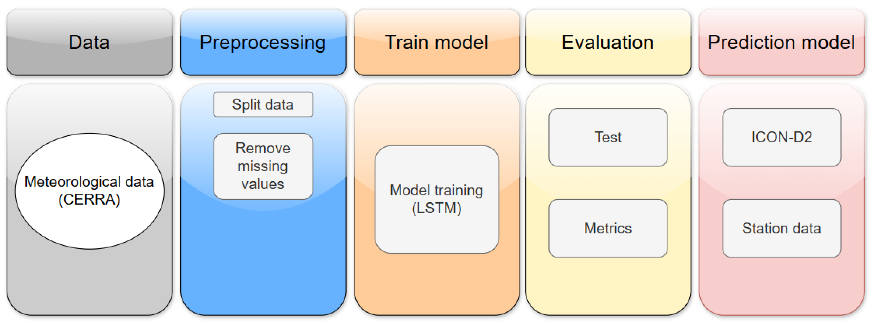
Theoretically, the weather prediction models in our study were obtained by a workflow of the processes illustrated in Figure 5. The workflow demonstrates a systematic approach for developing an ML model for temperature prediction based on weather data [13]. Here, the weather forecasting starts with acquiring meteorological data from the CERRA datasets. These meteorological data are then entered into the preprocessing step, where issues such as missing values are eliminated, improving data quality and preparing them for processing with various ML methods. Typically, model training using RNN, LSTM, or GRU NNs serve for weather prediction purposes. The next step presents an evaluation of the model, in which the quality of the created model is estimated. As a final step, the optimal model based on evaluation metrics is chosen, and used as the prediction model, supplemented with the ICON-D2 dataset and real weather data from a mobile weather station to perform continuous forecasts.

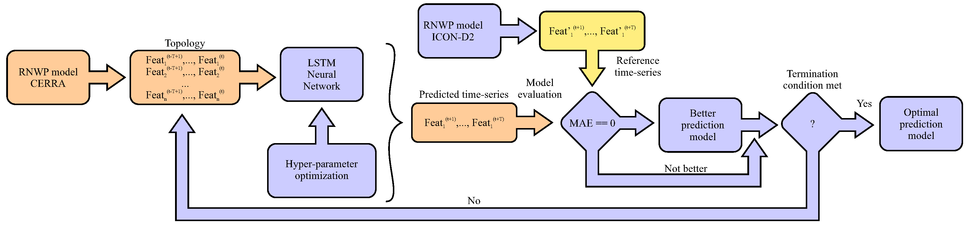
The proposed prediction method, Maximus, consists of two phases: modeling (also learning) and simulating (also predicting) the air temperature [28]. The purpose of the first phase is to find the optimal prediction model, while the purpose of the second phase is to test this prediction model in a real situation. In Figure 6, the Maximus model learning is presented, which is divided into more steps as follows: Extracting weather features from the RNWP model CERRA [16] is conducted first. Interestingly, the extracting is performed manually in the so-called generations, where different sets of available features in the CERRA dataset are selected for the LSTM input, in order to establish which features are more important for predicting the air temperature, and thus determines the topology of the LSTM network. Next, the optimization of LSTM hyper-parameters follows, where the optimal architecture of the NN is searched for. The result of this step is the prediction model that needs to be evaluated. In the evaluation step, the predicted time-series generated by the RNWP model ICON-D2 is constructed and serves as the reference prediction model. When the proposed predicted air temperature time-series is better than the reference one, according to the evaluation metrics discussed in the remainder of the paper, it is announced as the new best prediction model. Finally, at the end of the optimization, the last best prediction model is taken as a Maximus optimal prediction model.

The input to the LSTM network in the proposed method is defined as a set of features from the CERRA dataset in the learning phase that are preprocessed to similar names of the features as found in the CERRA dataset. Obviously, the set of features can be set manually by the developer. Actually, the task of the LSTM network is to predict the future values of the air temperature from the sequences of the past data captured in the last T hours. Obviously, the ICON-D2 dataset supports the similar names of the features as the CERRA that allow us to compare both time-series (i.e., reference and proposed) fairly.

In general, the method “Sliding Window” (SW) is applied, where the future sequence of T feature’s values are predicted from the past T feature’s values, as follows:

$$\underset{\mathrm{Past}}{\underbrace{\left.\begin{array}{c}Fea{t}_1^{(t-T+1)},\dots ,Fea{t}_1^{\left(t\right)}\\ \dots \\ Fea{t}_N^{(t-T+1)},\dots ,Fea{t}_N^{\left(t\right)}\end{array}\right\}}}⟹\underset{\mathrm{Future}}{\underbrace{Fea{t}_1^{(t+1)},\dots ,Fea{t}_1^{(t+T)}}},$$

(1)

where there is a sequence of history data for features $Fea{t}_i^{\left(t\right)}$ for $i=1,\dots ,N$ denotes the past values at time t that serve to predict the future values from the $Fea{t}_1^{(t+1)}$ to the $Fea{t}_1^{(t+T)}$, while the parameter N is the number of features and the parameter T the number of packets within the sequence. Indeed, the feature can be predefined more precisely by a sequence of the past values higher than those prescribed by the parameter T. This characteristic is described by the introduction of a parameter ‘SW size’, which is normally set to the value T. When a behavior of a particular k-th feature $Fea{t}_k^{\left(t\right)}$ is observed in $T=24$ instead of $T=12$ h periods, the parameter ‘SW size’ needs to be set to the value 24. Obviously, the number of time sequences for the learning phase depends on the number of considered years.

In our study, the LSTM network was used for prediction of the air temperature on micro-locations due to a vanishing gradient problem by back-propagation [29]. Thus, the arbitrary long-term dependencies are not tracked in the input sequences. In place of the back-propagation, the LSTM network is trained with a set of training sequences using the optimization algorithm gradient descent, combined with back-propagation through time. These algorithms modify the weights of the LSTM network in proportion to the derivation of the error [6]. During the training phase, early stopping is used to prevent the model from over-fitting. The Learning-Rate (LR) Scheduler helps to adjust the LR during training and aids in faster convergence and better model performance. The system also saves the best model periodically. At the end of training, the model with the lowest Mean Absolute Error (MAE) values is selected based on selection of the parameters. After that, model prediction and evaluation are performed, where the best model is constructed and trained, and predictions are made.

The LSTM network is controlled by setting the following hyper-parameters [30]:

• Number of nodes and hidden layers: The layers between the input and output layers are called hidden layers.
• Number of units in a dense layer: A dense layer is the most frequently used layer, which is basically a layer where each neuron receives input from all the neurons in the previous layer.
• Dropout: Every LSTM layer should be accompanied by a dropout layer that helps avoid overfitting in training by bypassing randomly selected neurons, thereby reducing the sensitivity to specific weights of the individual neurons.
• Activation function: Activation functions play a critical role in neural networks by introducing non-linearity, which enables the network to learn complex patterns in data. There are a lot of various activation functions in DL, where the Rectified Linear Unit (ReLU) is the most popular and widely used due to its simplicity and effectiveness.
• Learning rate: The hyper-parameter $LR$ defines how quickly the network updates its parameters. Usually, this hyper-parameter has a small positive value, mostly in the interval $LR\in [0.0,0.1]$. To handle the complex training dynamics of recurrent neural networks better, adaptive optimizers are recommended (such as Adam in our study).
• Number of epochs: One of the critical issues while training a neural network on the sample data is Overfitting. To mitigate overfitting and increase the generalization capacity of the neural network, the model should be trained for an optimal number of epochs.
• Batch size: The batch size limits the number of samples to be shown to the network before a weight update can be performed.

The Maximus model’s performance is evaluated using two well-known statistical metrics, i.e., Mean Absolute Error (MAE) and Mean Square Error (MSE). Let us mention that the MAE metric is used for measuring the average magnitude of errors in a set of predictions according to the following equation:

$$MAE={\displaystyle \frac{1}{T}}\sum _{i=1}^T\left|y_i-x_i\right|,$$

(2)

where $y_i$ denotes the prediction value, $x_i$ the true value, and T is the number of observation values. The lower the MAE, the better the model fit. The MSE metric is defined as follows:

$$MSE={\displaystyle \frac{1}{N}}\sum _{i=1}^N{\left(y_i-x_i\right)}^2,$$

(3)

where the meaning of the variables $y_i$ and $x_i$ are the same as in the case of Equation (2). Also here, the lower the MSE, the closer to the actual values and the better the model’s accuracy. In general, the MSE measure indicates more sensibility to observations that deviate more from the means.

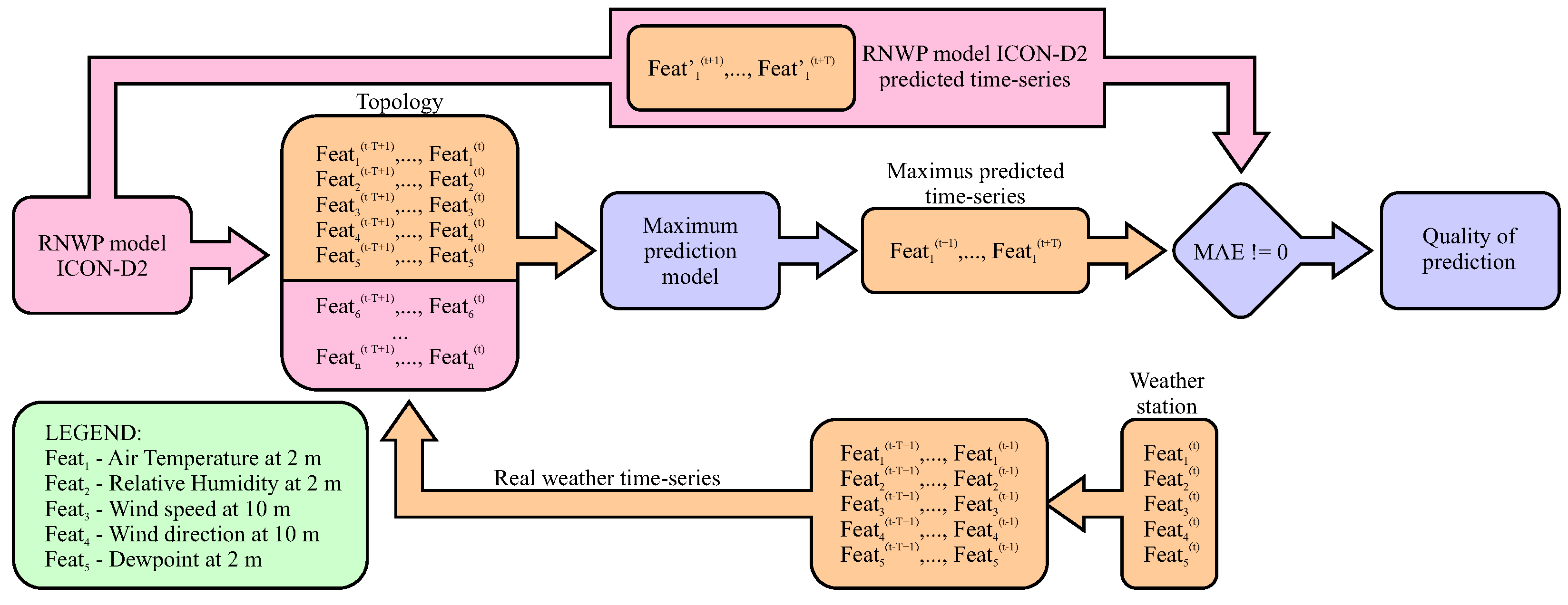
The intention of the learning phase was to improve the air temperature forecasts for the next 12 h for a given micro-location predicted by the ICON-D2 reference model, by using the optimal prediction model enriched with real meteorological ICON-D2 weather data, as provided by the mobile weather station. The prediction is presented as the flow diagram in Figure 7. where the example considers the N feature values that enter as inputs nto the Maximus prediction model, and thus defines the topology of the LSTM network. The selected set of features is extracted from two different sources: (1) the mobile weather station, and (2) the ICON-D2 higher-resolution dataset. Let us assume the mobile weather station is given that consists of five sensors. The features acquired from these sensors (i.e., air temperature, air pressure, relative humidity, wind speed, and rainfall intensity) are denoted as ‘Feat_1’ to ‘Feat_5’, as can be seen from the legend in the figure. Actually, the first five inputs to the LSTM network are taken from the mobile weather station by merging the $T-1$ past feature values with the current values, while the remaining $N-5$ features enter from the RNWP model ICON-D2 to the Maximus prediction model unchanged.

The result of the Maximus prediction model is the predicted time-series of air temperatures for the next T hours. Finally, the time-series predicted by the Maximus is compared with the time-series for the next T hours as predicted by the ICON-D2 reference model according to the statistical measure MAE, in order to determine the deviance between both. Let us emphasize that the MAE cannot be treated in the same way as in modeling case, because now the following holds: The higher the MAE value, the more powerful the Maximus prediction at the specific micro-location.

On the other hand, if the value of MAE is zero, it seems, there is no need for using the special prediction model for micro-locations. However, this problem can also be viewed from another perspective: In the case that the prediction models could have integrated physics indicators (i.e., the common indicators included in all weather prediction models), together with micro-physics indicators of a particular micro-location (e.g., turbulence caused by local wind; influence of relief, like altitude, atmospheric overheating, etc.), such models reflect the characteristics of the micro-location as a whole (i.e., ensure that MAE ≠ 0) and therefore could be tested on a regional level together with the specific micro-physics indicators. Moreover, if we could change the micro-physics indicators of the model by ourselves, such models could predict air temperature for the specific micro-location more accurately. Unfortunately, this development is connected also with additional resources and, therefore, remains a future direction in this moment.

Thus, the reference data were aggregated from the ICON-D2 dataset, starting at a specific start time during the next 12 h. Interestingly, there is a little discrepancy between the sampling times of weather data entered in the ICON-D2 dataset, where the weather data are predicted on an hourly basis but refreshed in three hour intervals, and either the CERRA dataset or mobile weather station, where these data are sampled on an hourly basis.

The meteorological station data from our autonomous professional weather station are very important, as they contribute hugely to the prediction of the air temperature. Indeed, there are only a limited number of features that are able to serve as an input to the LSTM network. Consequently, the missing features need to be supplemented from the ICON-D2 dataset. The experiments and obtained results are discussed in detail in the remainder of this paper.

4. Experiments and Results

The goal of our experimental work was to show that the Maximus can predict the air temperature at micro-locations using modern ML methods more accurately than by using general weather forecasting models. The prediction was performed using the LSTM NN. In line with this, various experiments were conducted with different LSTM topologies, hyper-parameter optimizations, and evaluation metrics. Three sources of the input weather data were taken into consideration during our experiments: (1) the lower-resolution CERRA dataset for LSTM learning, (2) the higher-resolution ICON-D2 dataset for evaluation and simulation, and (3) real weather data obtained from a mobile meteorological station capturing the current weather conditions at a specific micro-location.

In this study, the air temperature was predicted for $T=12$ h in the future using LSTM networks and various SW sizes. These networks are very complex for real applications due to a lot of hyper-parameters, various LSTM topologies, and even the quality and quantity of the training data. Indeed, all these issues in the application of the LSTM need to be tuned during the large experimental work.

The experiments were run on a personal computer with the characteristics as shown in

Table 5. Hardware and software characteristics of the computer, on which experiments were run.

Measuring Range	Description
Type	LENOVO IdeaPad L340-15 FHD
CPU	Intel Core I5-9300H
RAM	8 GB
GPU	GeForce GTX 1050
SW	Python 3.10.13 libraries math, sklearn

.

The measurement site is equipped with a fully automated personal weather station. The station is installed on natural terrain, surrounded by grass and a garden, with the nearest village located several kilometers away and a lack of significant urban infrastructure. This rural setting minimizes anthropogenic influences on the recorded data. The station follows a fixed placement strategy to ensure the consistency and representativeness of atmospheric conditions: sensors are mounted according to manufacturer-recommended heights and clearances to avoid obstructions and localized bias. All sensors are calibrated before deployment using reference instruments, and periodic validation checks are conducted to ensure long-term accuracy. The station is configured for real-time monitoring, automatically recording meteorological parameters and transmitting data to a secure cloud platform at 10 min intervals. This setup enables continuous data availability and supports quality control procedures based on automated range and consistency checks. These details have been added to the revised Methods section to clarify the observational framework.

In practice, the Maximus proposed methods were implemented as follows: At first, the sensors sent data via cable to the central unit. The central unit has ports open for specific sensors. When connected, it has LCDs, which show if the sensors have successfully connected and recognize them, as well as any errors that appear. The central unit has a 4G-supported SIM card inside (cellular network), which periodically, specifically around every 10 min, connects to the cloud and sends data written to the database for the last 10 min.

Two experiments were conducted, as follows:

• Searching for the Maximus optimal air temperature prediction model;
• Comparison of the Maximus optimal air temperature predicted by the indicated optimal prediction model with the reference based on the higher-resolution ICON-D2 dataset.

The experiments are described in detail in the remainder of this paper.

4.1. Searching for the Optimal Air Temperature Prediction Model

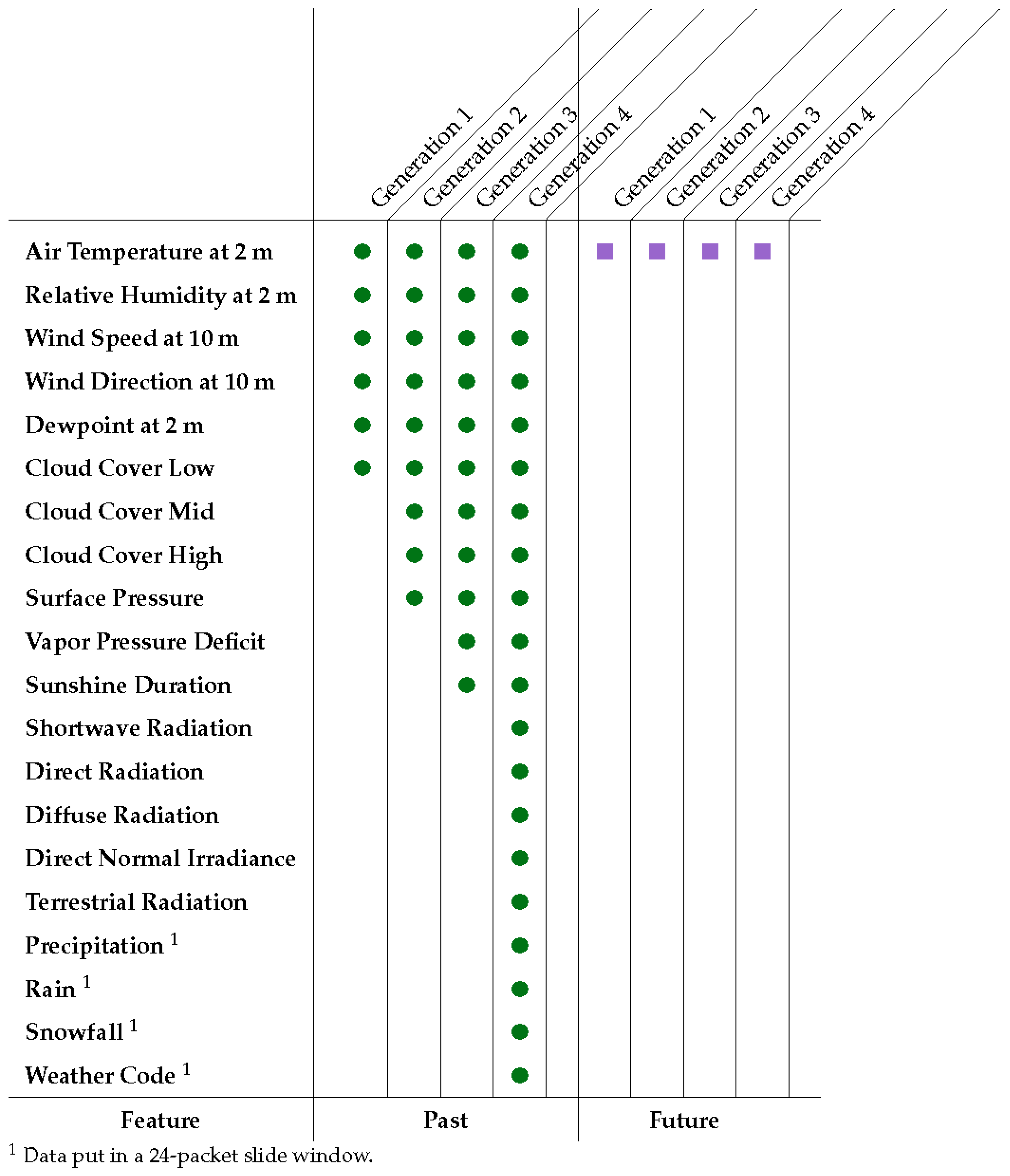
In the first experiment, the Maximus optimal model for the prediction of air temperature was searched for. At first, the best LSTM topology was indicated by the developer; then, the optimal hyper-parameters were determined, and, finally, the proposed prediction model was evaluated according to the MAE metric. The more appropriate LSTM topologies were determined in four generations, where sequences of past data for different sets of features and different SW sizes per feature were captured at the input layer on an hourly basis (Figure 8). Thus, the output layer is unique in all cases, and consists of T future values. No data was found on the satellite source of the weather model. It is incorporated into both models through data assimilation beforehand, so we obtained prepared data for that. So, in situ observations and satellites provide weather data with data assimilation techniques.

As can be seen in Figure 8, the generations differ between each other in the number of features, as found in the lower-resolution CERRA dataset placed in the input layer as the past data. Let us mention that there are a lot of feature variables divided into different categories [31], where only a specific set of these were selected for the particular generation. The presence of the definite feature entered at the LSTM input in a specific generation is denoted with a green circle in the table. For instance, six various features were employed in Generation 1, while even 21 features determine the predicted air temperature in Generation 4. Depending on the generation, the number of inputs from the RNWP model ICON-D2 varies from generation to generation. The more reliable inputs are therefore expected in Generation 1, where only one input is taken from the predicted RNWP model ICON-D2, while the remainder of the inputs are pure real values. On the other hand, the feature ’Air temperature at 2 m’ arises as the future data in all the observed generations. This fact is denoted with the corresponding violet squares in the table.

Interestingly, each feature emerging at the input layer enters as a time sequence consisting of observations (also packets) captured on an hourly basis. Actually, the number of observations is determined by the SW size per feature. Let us assume that we support $T=12$ observations per day. Then, the number of observations at the input/output layers per generation is that presented in

Table 6. Number of observations at input/output layers.

Layer	Generation
	1	2	3	4
Input layer	72	108	132	288
Output layer	12	12	12	12
Total	84	120	144	300

. The total number of observations is added to the last row in the table. In summary, the total number of observations in Generation 1 is 72, because, for each of the six features, we have $T=12$ observations per feature, which amounts to $6\times 12=72$ in total. In summary, the number of features increases by increasing the number of generations.

Tuning the hyper-parameters of the LSTM network was conducted after the scenarios illustrated in

Table 7. Number of runs by different hyper-parameter settings of the LSTM networks by generation.

Nr.	Parameter	Generation
		1	2	3	4
1	Number of LR	2	1	6	1
2	Number of nodes and hidden layers	1	1	9	1
3	Number of years for test data	3	1	1	1
4	Number of batch sizes	4	1	3	2
5	Number of captured years for the testing phase	3	1	1	1
6	Number of packets in the sliding window	1	1	1	2
∑	Number of configurations	72	1	162	4

. As is evident from the table, the optimal values of six hyper-parameters were searched for during the experimental work. These hyper-parameters were tuned by modifying the particular parameter in the number of different runs. For instance, the hyper-parameter ‘Number of nodes and hidden layers’ was tuned in one run per generation, except for Generation 3, where the hyper-parameter was modified in nine different configurations (i.e., the settings of the LSTM hyper-parameters). Interestingly, in the last row of the table, the total number of runs is presented, from which it can be observed that 239 different runs of different LSTM architectures were employed in the summary.

Finally, searching for the best configuration of the LSTM network was established by varying the hyper-parameters ‘Number of nodes and hidden layers’, ‘Dropout’, ‘Activation’, ‘Optimizer’, and ‘Dense’. In line with this, nine different configurations were defined. Actually, the parameter ‘Dropout’ has a crucial influence on the architecture of the LSTM network due to helping to avoid overfitting in training. The other hyper-parameters influencing the behavior of the LSTM network remained more or less fixed during the tuning process (

Table 8. Employed configurations of LSTM networks.

Configuration	No. of Units in the Hidden Layer	Dropout	Activation	Optimizer	Dense
1	32-16	(0.5.0.5)	‘relu’	Adam	n_lags_out
2	64-32	(0.5.0.5)	‘relu’	Adam	n_lags_out
3	128-64-64	(0.5,0.2)	‘relu’	Adam	n_lags_out
4	128-32	(0.5.0.5)	‘relu’	Adam	n_lags_out
5	64-32	(0.5.0.2)	‘relu’	Adam	n_lags_out
6	128-64	(0.5.0.2)	‘relu’	Adam	n_lags_out
7	128-64	(0.2.0.2)	‘relu’	Adam	n_lags_out
8	256-128	(0.2.0.2)	‘relu’	Adam	n_lags_out
9	256-128	(0.4.0.4)	‘relu’	Adam	n_lags_out

). As can be observed from Table 8, the LSTM employed configurations are designated with the numbers 1 to 9, and they are referenced accordingly in the remainder of the paper. The hyper-parameter ‘Dropout’ refers to the specific hidden layer, while its default value was normally set to the value 0.5. The activation function ‘ReLU’ was used in our experimental work, which allows the LSTM network to learn nonlinear dependencies. Adam is an optimization algorithm that can be used instead of the classical stochastic gradient descent procedure, to update LSTM network weights iteratively based in training data. The neurons of the dense layer are connected to every neuron of its preceding layer. In our case, the number of the dense layer is equal to the number of nodes at the output layer (i.e., n_lags_out = 12).

The results obtained in different generations are discussed in detail in the remainder of the section. Let us mention that only the more prominent runs are presented in

Table 9. Model performance in Generation 1.

Run	Epochs	Batch	Conf.	Years	SW Size	MAE	MSE
13	30/30	32	1	5	12	1.2205	2.3841
14	300/34	32	1	5	12	1.2327	2.3185
15	300/52	32	1	1	12	1.1232	1.9552
16	300/41	64	1	1	12	1.0912	2.0472
17	300/38	64	1	1	12	0.9619	1.6091
18	300/60	128	1	1	12	0.6694	0.8425
19	300/96	128	1	1	12	0.6575	0.7791
20	300/124	128	1	1	12	0.5933	0.6624
21	300/79	256	1	7	12	0.5272	0.5349
22	300/56	64	1	7	12	0.9258	1.5472
23	300/186	64	1	1	12	0.4902	0.4945
24	500/73	128	1	1	12	1.1418	2.2701
25	500/202	64	1	1	12	0.4958	0.5052

,

Table 10. Model performance in Generation 2.

Run	Epochs	Batch	Conf.	Years	SW Size	MAE	MSE
1	500/204	64	1	1	24	0.0390	0.0029

and

Table 11. Model performance in Generation 3.

Run	Epochs	Batch	Conf.	Years	SW Size	MAE	MSE
1	500/191	64	1	1	12	0.4872	0.4744
2	500/191	256	1	1	12	0.5054	0.4899
3	500/191	64	2	1	12	0.4832	0.4591
4	500/56	32	2	1	12	1.0342	1.7020
5	1000/65	64	3	1	12	6.6885	1408.1392
6	1000/86	64	4	1	12	3.2257	71.2232
7	1000/52	64	4	1	12	1.0425	1.7856
8	500/83	64	5	1	12	1.1034	2.1194
9	500/56	32	5	1	12	1.4214	3.2940
10	500/191	32	5	1	12	7.3464	75.3324
11	500/51	32	5	1	12	0.7645	1.0179
12	500/37	64	6	1	12	0.6255	0.7027
13	500/87	64	6	1	12	0.5832	0.6554
14	500/77	64	6	1	12	2.2373	3816.9081
15	500/84	64	6	1	12	0.5932	0.6437
16	500/78	64	6	1	12	0.5993	0.6845
17	500/61	64	7	1	12	0.6286	0.7132
18	500/68	64	7	1	12	1.1527	2.2816
19	500/51	64	8	1	12	0.5642	0.5929
20	500/56	64	9	1	12	0.6523	0.7590
21	500/52	64	8	1	12	0.5638	0.5888
22	500/69	64	2	1	12	1.0129	1.6512
23	500/75	64	2	1	12	0.9464	1.5135
24	500/100	64	2	1	12	0.5288	0.5484
25	500/100	64	2	1	12	0.5164	0.5186
26	500/100	64	2	1	12	0.5301	0.5437
27	500/101	64	2	1	12	0.4966	0.4862
28	500/107	64	2	1	12	0.4948	0.4753
29	500/78	64	2	1	12	0.9456	1.4490

. Actually, Generation 1 of the documented learned models (Table 9) was characterized by having the same NN configuration. In total, 13 different runs and 72 more interesting runs are aggregated into the table, which is divided into columns as follows: The column ‘Run’ denotes the sequence number of a performed LSTM execution for the particular NN architecture. The runs are distinguished between each other with regard to the number of epochs (column ‘Epochs’), batch sizes (column ‘Batch’), adaptation algorithm (column ‘Optimizer’), and number of packets within the SW (column ‘SW size’). Thus, the hyper-parameters, like the architecture of the LSTM network (column ‘Architecture’), and number of years of test data (column ‘Years’) were fixed during the experiments. Let us emphasize that the column ‘Epochs’ reports two values, where the first one designates the value of the hyper-parameter Epoch, while the second value is the real number of epochs before the LSTM networks stopped due to overfitting. The last two columns, ‘MAE’ and ‘MSE’, represent the results obtained according to the measures MAE and MSE, respectively. Let us mention that the same structure was applied for the tables representing the results of the other generations as well. The best results in the Generation 1 are presented in bold in Table 9.

The main differences between runs occurred in the number of epochs, the batch size, and the number of years captured for training. Actually, all the runs employed the LSTM configuration. In summary, the best model according to the metrics MAE and MSE was produced in run 23, where the number of epochs was set to the value 300, the batch size to 64, and only data acquired in one year were set for training the LSTM network. The following conclusions are evident by analyzing the results in

Table 12. Model performance in Generation 4.

Run	Epochs	Batch	Conf.	Years	SW Size	MAE	MSE
1	500/75	64	2	1	12	0.3191	0.1846
2	500/76	32	2	1	12	0.3008	0.1669
3	500/123	32	2	1	24	0.2907	0.1706
4	500/500	32	2	1	24	0.2815	0.1609

: (1) the higher the number of years for learning data, the worse the prediction; (2) the higher values of batch sizes (e.g., 250, 128) did not necessarily lead to a better prediction; and (3) although the hyper-parameter ‘Batch size’ = 500 was also employed during the experimental work, the results were not improved significantly compared with the runs using the lower values of this hyper-parameter.

For Generation 2 of the learned models (Table 10), the focus was on forward prediction based on visible past and future data, where the results of the metrics MAE = 0.0390 and MSE = 0.5052 improved significantly compared to the values achieved in the previous generations, while, at the same time, the time complexity was increased before the model converged. Let us mention that only one configuration was tested in Generation 2. As can be concluded from the results in the table, these were improved mainly at the expense of increasing the hyper-parameter ‘SW size’ to the value of ‘SW size’ = 24. Thus, the hyper-parameters ‘Epochs’, ‘Batch size’, ‘Architecture’, and ‘Years for testing phase’ were fixed to the already-found optimal values. The best results in Generation 2 are presented in bold in Table 10.

Generation 3 (Table 11) was devoted to highlighting the dependence between different hyper-parameters of the LSTM networks. In line with this, the number of epochs was set to higher values, i.e., ‘Epochs’ = {500,1000}, while the batch size was mainly fixed to 64, which was found to be the optimal value in the previous experiments. This generation is distinguished from the others due to comparing different LSTM configurations. The hyper-parameters and ‘Years’ were fixed to the values 1 year and 12 years, respectively. The best results for Generation 3 are presented in bold in Table 11.

As is evident from the table, the best model was found in run 1, where the metrics MAE = 0.4873 and MSE = 0.4742 were achieved by employing the LSTM of Configuration 1. Interestingly, significant deviations can be observed in the $\mathit{MAE}$ and $\mathit{MSE}$ metrics designated by values in the red color (i.e., runs 5, 10, 14). This is because, here, a lot of experimentation was devoted to modifying the internal metrics, such as the LR and the architecture of the neural network, by removing and adding different layers, as well as neurons. Typically, these models suffered from an overfitting that arose when the model contained more parameters than could be justified by the data.

In Generation 4 of the learned model settings (Table 12), some of the best models are presented that reached this level with certain settings. Typically, these models were obtained by using the LSTM Configuration 2 and a batch size of 32. Interestingly, the best results according to the metrics MAE = 0.2815 and MSE = 0.1609 were obtained in run 4, where the number of epochs was set to the value 500, the number of years for testing set to 1, and the SW size to 24. Interestingly, these results were obtained by maximizing the real number of epochs to 500. The best results for Generation 4 are presented in bold in Table 12.

Let us emphasize that the best results for this particular generation are best for the specific values due to the same configuration hyper-parameters. In general, the best results are hard to find because of variable weather conditions, i.e., each weather situation has another starting condition that strongly influences our model’s prediction. The variances are substantial within the exact prediction, which can happen in one hour.

4.2. Comparison of the Maximus Optimal Air Temperature Prediction Model with the Reference Model ICON-D2 Dataset

The aim of the second experiment was to verify the Maximus optimal models as found during the first test in a real environment.

Table 13. Overview of the metrics for the predictive model of Generation 1 obtained in run 23.

Start		End		T	MAE		${\mathit{r}}_{\mathbf{Maximus}}$	${\mathit{r}}_{\mathbf{\text{ICON-D}}2}$
Date	Time	Date	Time	[h]	Maximus	ICON-D2
03.1.2024	19:00	04.1.2024	06:00	12	0.9	1.1	0.6282	0.1343
04.1.2024	10:00	04.1.2024	21:00	12	3.9	1.9	0.8325	0.9943
08.1.2024	9:00	08.1.2024	20:00	12	2.0	0.5	−0.4049	−0.6946
09.1.2024	11:00	09.1.2024	22:00	12	0.4	0.8	0.6592	0.6188
n/a	n/a	n/a	n/a	12	1.23	1.15	0.42875	0.2632

,

Table 14. Overview of the metrics of the predictive model of Generation 2 obtained in run 1.

Start		End		T	MAE		${\mathit{r}}_{\mathbf{Maximus}}$	${\mathit{r}}_{\mathbf{\text{ICON-D}}2}$
Date	Time	Date	Time	[h]	Maximus	ICON-D2
08.1.2024	18:00	09.1.2024	05:00	12	0.4	0.7	0.7051	0.7244
09.1.2024	20:00	10.1.2024	07:00	12	1.2	1.9	0.5386	0.5159
10.1.2024	22:00	11.1.2024	09:00	12	0.7	1.8	0.9765	0.8411
11.1.2024	07:00	11.1.2024	18:00	12	0.8	1.5	0.9875	0.9781
n/a	n/a	n/a	n/a	12	0.8	1.5	0.8019	0.7649

and

Table 15. Overview of the metrics of the predictive model of Generation 4 in run 4.

Start		End		T	MAE		${\mathit{r}}_{\mathbf{Maximus}}$	${\mathit{r}}_{\mathbf{ICON-D}2}$
Date	Time	Date	Time	[h]	Maximus	ICON-D2
11.1.2024	19:00	12.1.2024	6:00	12	0.4	0.8	0.8540	−0.1679
15.1.2024	22:00	16.1.2024	9:00	12	1.4	1.2	0.8624	0.7031
17.1.2024	14:00	18.1.2024	1:00	12	4.6	2.9	0.8761	0.6522
20.1.2024	20:00	21.1.2024	7:00	12	0.7	1.3	0.9459	0.9099
n/a	n/a	n/a	n/a	12	1.8	1.6	0.8846	0.5243

show the MAE metrics of a particular version denoted as the Maximus model, which are compared with the MAE of the reference ICON-D2 model. Additionally, the results of both models are compared according to the Pearson correlation coefficient, indicating a relationship between the observed and predicted time-series. The Pearson coefficient values are drawn from the interval $r\in [-1,1]$, where $r\ge 0.5$ indicates a large positive relationship between the observed and predicted time-series: $r\in [0.3,0.5)$ medium, $r\in [0.1,0.3)$ small, and $r<0.1$ very small. Indeed, three models with different LSTM architectures were observed in the comparative study.

Table 13 aggregates the results of the comparative study between the Maximus optimal and the ICON-D2 reference model. Thus, the prediction model of Generation 1 obtained in run 23 (i.e., the best model in Table 9) was taken into consideration. There are four predictions presented capturing data from 3.1.2024 till 9.1.2024 in 12-h periods of time. As can be seen from the table, the MAE metric shows that the best learned model had worse results than the MAE metric obtained by the ICON-D2 model, while the comparison according to the Pearson coefficients shows the opposite, i.e., the air temperature time-series of the proposed predicted model matched the observed time-series more than of the ICON-D2 model.

Table 14 illustrates the results of the comparative study between the Maximus proposed and ICON-D2 reference prediction models, where the proposed model of Generation 2 obtained in run 1 was taken into closer consideration. Obviously, the optimal proposed model in Table 10 was employed in the study. As is evident from the table, the four weather predictions were illustrated with data captured from 8.1.2024 to 11.1.2024, while the results according to the MAE metric as obtained with the ICON-D2 reference model are slightly worse than those obtained by the best prediction model Maximus. The finding is also justified by the Pearson correlation coefficients, where the $r_{\mathrm{Maximus}}=0.8019$ is slightly higher than the $r_{\text{ICON-}\mathrm{D}2}=0.8019$, although both indicate a large positive relationship between the observed and predicted air temperature time-series.

Finally, the results of the comparative study found by the best prediction model Maximus of Generation 4 obtained in run 4 (Table 12) and the ICON-D2 reference model showed similar results to those in the first experiment, i.e., the MAE metric obtained by the Maximus optimal proposed model was slightly worse that obtained by the ICON-D2 reference model, but the Pearson correlation coefficients showed the opposite, i.e., $r_{\mathrm{Maximus}}$ > $r_{\text{ICON-}\mathrm{D}2}$.

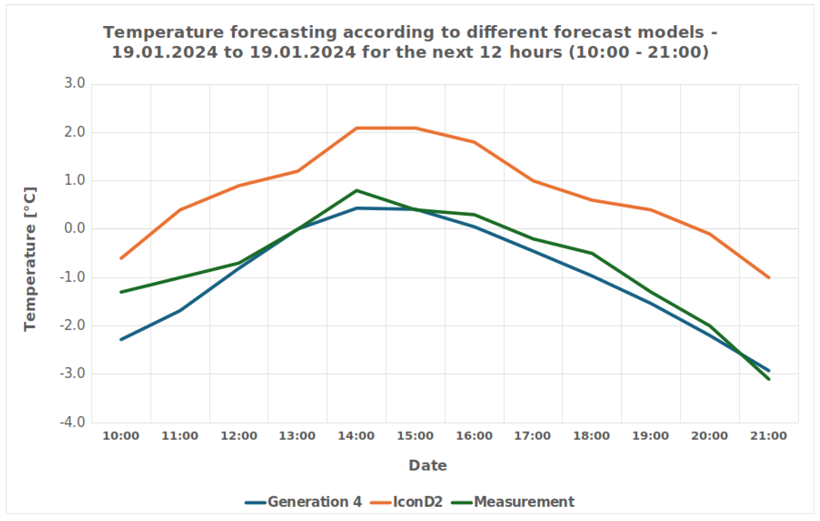
As the forecast models were improved, a specific weather situation was chosen for testing. On the selected day, 19.1.2024, it snowed in the morning, clouded up in the afternoon and cleared up gradually in the evening. The comparison between the forecast model and the reference model is presented in Figure 9, which depicts a graph with three lines as follows: (1) the blue line shows the forecast of the reference model, (2) the red line shows the real measurements of the meteorological station, and (3) the green line shows the results of the forecast model.

The graph justifies our hypothesis that the proposed prediction model can be used for the prediction of air temperature at micro-locations, because the PROP model (the blue line) predicted the temperature more reliably than the ICON-D2 reference model (the green line) compared with the real situation measured by the local meteorological station (the red line).

4.3. Discussion

The metrics we have used are important for evaluating and comparing forecast models, but they are far from indicative of the actual forecast error. One of the major problems is that we use historical meteorological station data as an input to the forecast model, and, at the same time, future reference model data, which can propagate the reference model error. The choice of parameter combination and time frame are very important here. If we choose the air temperature of the reference model as input to the forecast model, and we know that we are forecasting the air temperature, if the reference model has a large error, this will be reflected in our final result. Therefore, we need to choose ICON-D2 parameters that will not affect our final predictor variable directly. However, it is worth noting that this model is only trained to forecast at a given micro-location, whereas ICON-D2 covers data for the whole of Slovenia and its surroundings.

Another problem with ICON-D2 weather model is that although this is able to predict the air temperature on hourly basis, it is refreshed every 3 h, whereas we need to update our prediction model every hour. At the same time, we want to keep calibrating the forecast already produced by the ICON-D2 model. This can make it easier to detect a sudden drop or rise in air temperature that may not be detected by the model. Such forecasts come in very handy when forecasting an increasing number of extreme weather events. Ideally, data from satellite images should be retrieved every 15 min and fed into the forecast model. Also, the use of a radar image of rainfall intensity with an interval of 5 min could help to train the model even more optimally, and to compare the forecast of rainfall intensity with the ICON-D2 weather model. The use of a solar irradiance sensor, which is not present at the measuring station, could also make a decisive contribution to a better forecast. Also, a webcam that could predict what the weather is like using DL, and could help to obtain a better overview of the weather conditions.

Let us emphasize the time complexity of the proposed prediction method, Maximus. Although we are not focusing just on this component, it can be estimated that each learning phase in searching for the prediction model lasts approximately about 3 h. On the other hand, the proposed meteorological station is a mobile and independent of an external source of energy. This means that it is also flexible because the observed micro-locations could be changed easily by moving the location of the station. However, the prediction model needs to be updated properly by the moving.

The following seven advances of the proposed prediction method Maximus can be revealed:

• Use of Mobile Weather Station Data: The model integrates real-time, high-resolution data from a professional mobile weather station, enabling localized and frequent updates every hour.
• Development of an LSTM-Based Prediction Model: A novel Long Short-Term Memory (LSTM) neural network was designed and optimized specifically for micro-location temperature prediction, outperforming general models in several cases.
• Use of a Lower-Resolution Long-Term Dataset (CERRA): Leveraging the CERRA dataset allows for incorporating long-term historical patterns, enhancing the robustness of predictions.
• Comparison with ICON-D2: The proposed model was rigorously tested against the state-of-the-art ICON-D2 reference model, demonstrating competitive or superior results in several forecast windows.
• Hyper-parameter Tuning and Generational Testing: Comprehensive experimental design included different generations of models, topologies, and hyper-parameter settings to identify optimal configurations.
• Flexibility and Portability of the Weather Station: The weather station setup is mobile and self-sustaining, which allows relocation and re-calibration for other micro-locations without major reconfiguration.
• Strong Statistical Evaluation: Model performance was evaluated using MAE, MSE, and Pearson correlation coefficient, ensuring accuracy and consistency were assessed.

On the other hand, the method’s limitations need to be summarized as follows:

• Limited Number of Input Parameters: The LSTM network uses a restricted set of input features, which may omit critical meteorological factors affecting temperature prediction, increasing the risk of Type II errors.
• Temporal Resolution Gap Between Datasets: Differences in sampling frequency (e.g., hourly for CERRA and hourly for ICON-D2, but refreshed on a 3 hourly basis) complicate synchronization and model integration.
• High Computational Complexity: Extensive model training and hyper-parameter tuning require significant computational resources and time (approx. 3 h per training phase).
• Model Overfitting in Some Configurations: Certain LSTM configurations showed overfitting and poor generalization, especially when the number of parameters outstripped the volume of training data.
• Lack of Broader Applicability: The model is tailored to a specific micro-location in Slovenia, limiting its direct applicability to other geographical areas without re-training and recalibration.

It is clear that a lot of improvements could be made to better grasp all the details of the micro-location into the model learning process as well as prediction process. We could argue that we don’t explicitly define the physics of the model and model resolution but it is all already integrated into the model in the learning phase, as well as the prediction phase. We just recognize the patterns to get as close as possible to the micro-location, where the weather station, as source of reliable data, helps a lot to achieve that goal.

5. Conclusions

In term of the research goal to gain the ability to learn a Maximus weather model that can predict the air temperature for a given micro-location, we have implemented it successfully. Simultaneously, we have trained several models and compared their results, and found that the proposed Maximus optimal model predicts the air temperature for the next 12 h much better in certain situations.The objectives about the research question have, thus, been accomplished successfully.

In summary, the following conclusions can be drawn from the results of our study:

• The primary advantage of the proposed prediction model Maximus against the reference ICON-D2 is reflected in the fact that the former employs data obtained from the mobile weather station, which are updated each hour.
• The proposed solution Maximus considers a longer history of the regional weather situation due to using the CERRA dataset.
• On the other hand, the weakness of the Maximus model is that it considers a limited number of LSTM input parameters. In line with this, the possibility of causing Type II errors is increased. However, this type of error can be reduced by extending the time sequences and increasing the number of input parameters. Unfortunately, both mentioned issues demand powerful hardware for processing.

Comparing different prediction models with different combinations of input data, the LSTM architecture and their corresponding hyper-parameter settings could help to improve the results even further. Improved training data could also help significantly in addressing this problem. It is also worth mentioning the possibility of implementing another DL model, or building on it with specific systems that would improve local air temperature changes in a very short time. Forecasting could also benefit from air temperature forecasts with an interval more frequent than one hour.

Let us mention only few promising directions for future work: The new DL methods should replace LSTM NN, like LSTM with CNN or BiLSTM. The new sensors for monitoring the weather condition could be included as inputs to LSTM NN. Also the number of packets into the sliding window could be increased. Maximus would be moved to the computer grid in order to increase the learning speed from 3 h to 10 min. Some preliminary tests were already conducted in this direction.