CNN-Transformer-BiGRU: A Pump Fault Detection Model for Industrialized Recirculating Aquaculture Systems

Featured Application

The model is mainly used for fault detection of pumps in industrial recirculating aquaculture.

Abstract

Background: Modern aquaculture is increasingly adopting industrialized recirculating aquaculture systems, in which the stable operation of its circulating water pump is essential. Yet, given the complex working conditions, this pump is prone to malfunctioning, so its timely fault prediction and accurate diagnosis are imperative. Traditional fault detection methods rely on manual feature extraction, limiting their ability to identify complex faults, and deep learning methods suffer from unstable recognition accuracy. To address these issues, a three-class fault detection method for water pumps based on a convolutional neural network, transformer, and bidirectional gated recurrent unit (CNN-transformer-BiGRU) is proposed here. Methods: It first uses the continuous wavelet transform to convert one-dimensional vibration signals into time–frequency images for input into a CNN to extract the time-domain and frequency-domain features. Next, the transformer enhances the model’s hierarchical learning ability. Finally, the BiGRU captures the forward/backward feature information in the signal sequence. Results: The experimental results show that this method’s accuracy in fault detection is 91.43%, significantly outperforming traditional machine learning models. Using it improved the accuracy, precision, and recall by 1.86%, 1.97%, and 1.86%, respectively, relative to the convolutional neural network and long short-term memory (CNN-LSTM) model. Conclusions: Hence, the proposed model has superior performance indicators. Applying it to aquaculture systems can effectively ensure their stable operation.

1. Introduction

With the greater demand and quality requirements of consumers for aquatic products, it is necessary to accelerate the transformation of freshwater fisheries through scientific and technological innovations [1,2]. The global market share of industrialized recirculating aquaculture systems (IRASs) has steadily increased due to its controllable environment, easy automation, and operational intelligence [3,4]. In a typical recirculating aquaculture plant, the water pump ensures a circulating flow of the water body, providing a suitable living environment for farmed organisms. How to efficiently detect equipment failure and safeguard this pump’s long-term stable operation is arguably very important.

Common faults of water pumps include impeller damage, blockage, motor burnout due to phase loss, and bearing wear and corrosion. In IRASs, however, impeller wear rarely occurs because there is no sediment in the water and most of its debris, such as feces and residual feed, are adequately filtered by the feces collector, micro-filter, and biological filter barrel. Likewise, since the control cabinet is equipped with phase-loss protection, the motor burnout phenomenon (due to phase loss) is also relatively rare. The most common fault is the bearing failure of the water pump, which can take several forms (

Table 1. Main forms of water pump bearing failure in industrialized recirculating aquaculture systems.

Fault Type	Phenomenon	Main Reason (s)	Characterization Signal
Abrasion	The surface size changes, and the ball is no longer smooth	Insufficient lubrication	Vibration signal
Crack	The bearing’s outer ring or inner ring has a notch or a crack	Overload	Vibration signal
Corrosion	Rust spots on parts	Chemical corrosion, electric corrosion	Vibration signal

).

As seen from Table 1, the most direct manifestation of bearing faults is an altered vibration signal, which is mainly expressed in two ways:

(1)

Increase in vibration amplitude: Under normal circumstances, the water pump bearing operates stably, with its vibration amplitude remaining at a relatively low and stable level. When the bearing incurs wear and corrosion, its clearance will increase, loosening the tight fit between the raceway and the balls or rollers. During the operation process, additional impact forces and vibrations are generated, substantially increasing the vibration amplitude.

(2)

Change in vibration frequency: When there is local damage to the bearing, such as one or more cracks on the surface of its balls or pits on the raceway, specific frequency components related to the bearing’s own structure and faults are generated. If the fit between the bearing and the shaft or the bearing seat becomes loose, this will decrease the vibration frequency.

In recent years, much research has emerged on equipment fault detection. Zan et al. [5] proposed a detection method using the variational mode decomposition (VMD) algorithm for early rolling bearing faults. In order to better extract effective features, Liu et al. [6] introduced a method of constructing features from the time-domain energy entropy values of modal components, then input those into a support vector machine (SVM) for the identification of rolling bearing faults. In another work, Hou et al. [7] took advantage of the multi-view manifold component feature extraction (MvMCFE) technique’s superiority in nonlinear feature extraction, to propose a fault detection method that combined it with an optimized SVM. Li et al. [8] used the particle swarm optimization (PSO) algorithm to optimize the SVM for the detection of motor bearing faults, while Wang et al. [9] used the random forest algorithm to detect faults in charging pile equipment. Using the K-nearest neighbors (KNN) algorithm as a basis, Yang et al. [10] proposed a fault diagnosis algorithm and monitoring system for the bearings of hydraulic turbine units. Finally, Lu et al. [11] combined the KNN algorithm and the Naive Bayes algorithm to effectively diagnose the faults of rolling bearings.

Most of the studies cited above relied on traditional machine learning methods, which can perform well at fault detection. Still, the fault features must be manually extracted, and they are easily affected by subjective human judgments. Anupam et al. [12] used Complete Ensemble Empirical Mode Decomposition with Adaptive Noise (CEEMDAN) to decompose the data, and then fused the long short-term memory (LSTM) and gated recurrent unit (GRU) neural networks to achieve accurate gear fault identification. Likewise, Jiang et al. [13] suggested an equipment fault detection method based on knowledge graphs and task learning, while Ma et al. [14] used the attention mechanism-based gated recurrent unit (AM-GRU) network to detect the faults of intelligent substation equipment. Lastly, Hao et al. [15] presented a multi-sensor method combining one-dimensional convolution with LSTM for the successful diagnosis of equipment faults. Wang et al. [16] employed the Empirical Mode Decomposition (EMD) method to preprocess the raw signals of the Magnetic Flux Leakage (MFL) and designed a wire rope defect diagnosis network based on the CNN-transformer. Cao et al. [17] integrated the core advantages of the LSTM and transformer architectures for real-time prediction and fault detection in engineering system tasks.

The above deep learning algorithms can automatically extract fault features and demonstrate high recognition accuracy. Yet, most of them are based on one-dimensional signals and lack features integrating the time domain with the frequency domain. To that end, Li et al. [18] adopted a multi-receptive field graph convolutional network: when extracting features, it integrates the information of adjacent nodes and fuses its own parameters, thereby improving the network’s overall performance. Tian et al. [19] developed a bearing fault diagnosis method that combines a frequency-domain feature extraction with a dual-stream convolutional neural network (CNN). Mo et al. [20] proposed a lightweight CNN network that fuses one- and two-dimensional features for equipment fault diagnosis; by researching the feature fusion of the time–frequency domain, those authors improved the model’s performance.

To sum up, progress is being made at improving the method of equipment fault detection, bringing it closer maturing. However, its application is still mostly restricted to standard industries, and its potential applications in the field of IRASs is unexplored and virtually unknown. Moreover, the environment of recirculating aquaculture factories is quite complex, and various factors, such as interference between equipment, water flow, impurities, and corrosion, could impair their water pumps’ fault detection. Aiming to tackle these problems, this paper proposes the convolutional neural network, transformer, and bidirectional gated recurrent unit integrated (CNN-transformer-BiGRU) model, whose key characteristics are anti-interference and high precision. This method first uses the continuous wavelet transform to convert one-dimensional vibration signals into time–frequency images. Then, it takes advantage of the CNN’s powerful ability to process images to extract local features in both time and frequency domains. Next, it utilizes the encoder in the transformer to improve the model’s hierarchical learning ability for features. Finally, it captures the front and back feature information in the vibration signal sequence via the BiGRU, to achieve the accurate detection of water pump faults under complex working conditions and background noise.

2. Materials and Methods

2.1. Network Model Structure

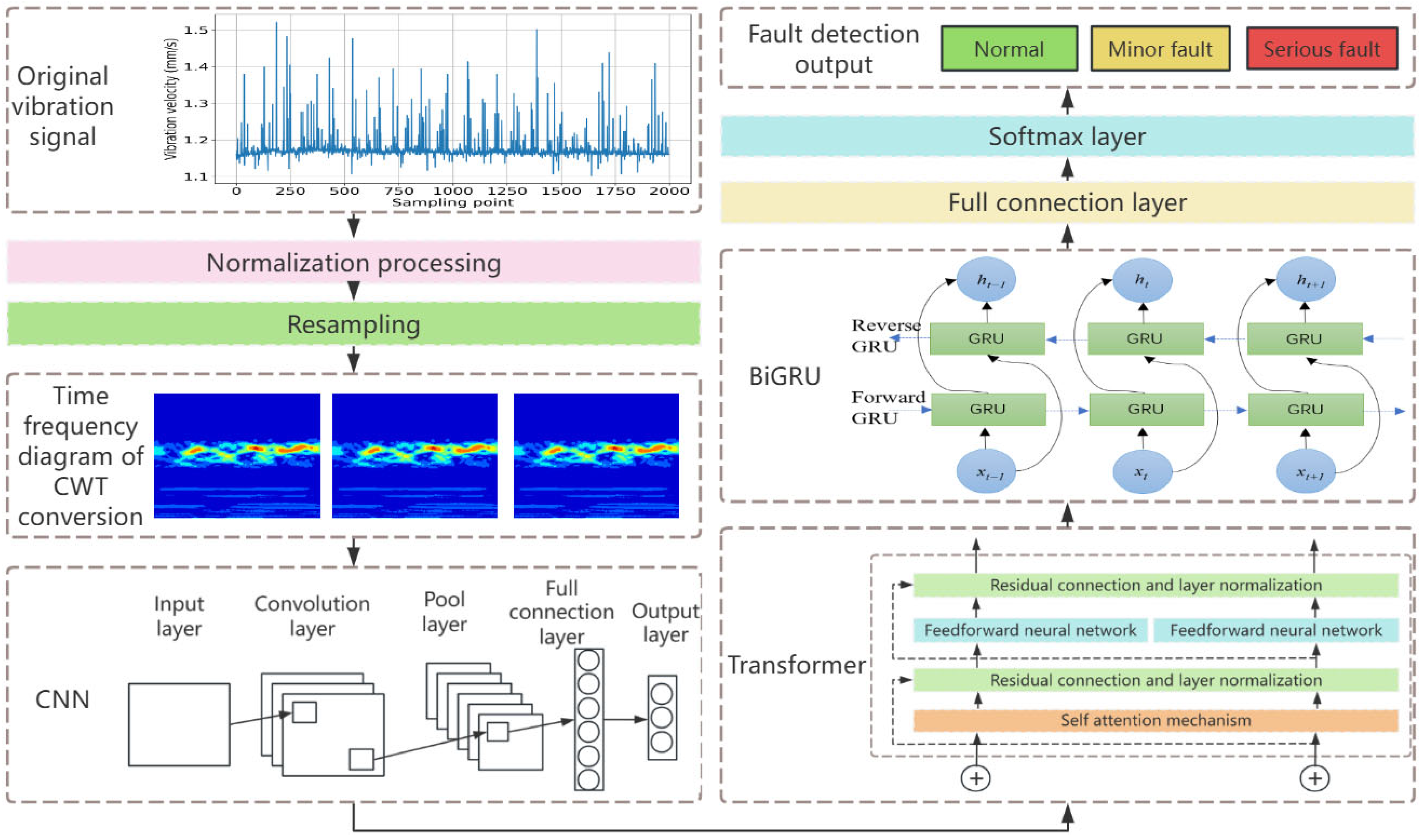
In the field of IRASs, a new network model (CNN-transformer-BiGRU) that is applied to the task of water pump fault detection is thus proposed. Its overall structure is illustrated in Figure 1.

To detect the water pump’s faults, its vibration signal data were collected via sensors, and then processed by normalization and resampling. To convert these one-dimensional vibration signals into image data that integrate the time and frequency domains, the continuous wavelet transform was used; a CNN then preprocessed the input data and extracted local features; after that, the data were fed into the transformer for global feature modeling. This output served as input into the bidirectional gated recurrent unit (BiGRU) network model for sequence modeling and processing. Finally, the fully connected layer and Softmax function output the classification results.

2.2. Sensor Selection

Through the analysis of potential fault causes, vibration signals of the water pump were monitored and its vibration data under different working conditions were obtained for experimental analysis. To collect these data, we chose the HG-ZD-20B integrated vibration sensor, whose detailed parameters are listed in

Table 2. Detailed parameters of the vibration sensor used in this paper.

Parameter Name	Description
Use environment	Temperature −40 °C~85 °C
Range	0–20 mm/s
Output	4–20 mA
Working voltage	DC 12–24 V ± 10%
Wiring mode	Two-wire system
Measurement direction	Vertical or horizontal
Accuracy	<F.S ± 1%
Resolving power	0.1 mm/s

.

The sensor was installed on the circulating water pump in the IRAS test area, using a magnetic suction base to affix it to the pump’s metal shell. The water pump model is 50WQ9-22-2.2, with a rated voltage of 380 V and a rated speed of 3000 r/min. This magnetic suction method is convenient for installing and quickly positioning the sensor at various monitoring points. By comparing different monitoring points, more distinctive signal data could be obtained.

2.3. Data Acquisition

The experimental data used in this paper were collected on-site in the IRAS test area of the Yangdu Base, Zhejiang Academy of Agricultural Sciences. The sensor was connected to the acquisition card, and in turn, the latter was connected to the computer for data collection and storage. HK_USB_DAQ is a high-speed data acquisition card based on the USB bus, with a maximum sampling rate of up to 100 kHz (

Table 3. Detailed parameters of the data acquisition card used in this study.

Parameter Name	Description
AD port	8-way differential/16-way single ended input
AD converter	12 bit AD
Sampling rate	Maximum single channel 100 kHz, maximum Multi-channel sampling rate = 50 kHz/Number of channels used
AD FIFO cache	10 K
AD acquisition mode	Single acquisition, intermittent acquisition, continuous acquisition
System accuracy	±1 LSB
Maximum common mode voltage	±10 V
Input socket	3.81 mm terminal blocks

).

We used the Python 3.8.3 programming language to develop the data collection functions. Since the vibration signal data of the water pump need to be continually recorded multiple times, the continuous collection function interface was used. The continuous Analog-to-Digital (AD) collection process is depicted in Figure 2, with the obtained vibration signal data then written into the disk file.

The vibration signals from the sensors are stored in a computer via a data acquisition card, which involves several steps: device initialization, sampling parameter configuration, cyclic data reading, temporary data buffering, file writing, and device shutdown. Among these, cyclic data reading and temporary buffering are critical for the high-speed signal acquisition of the data acquisition card.

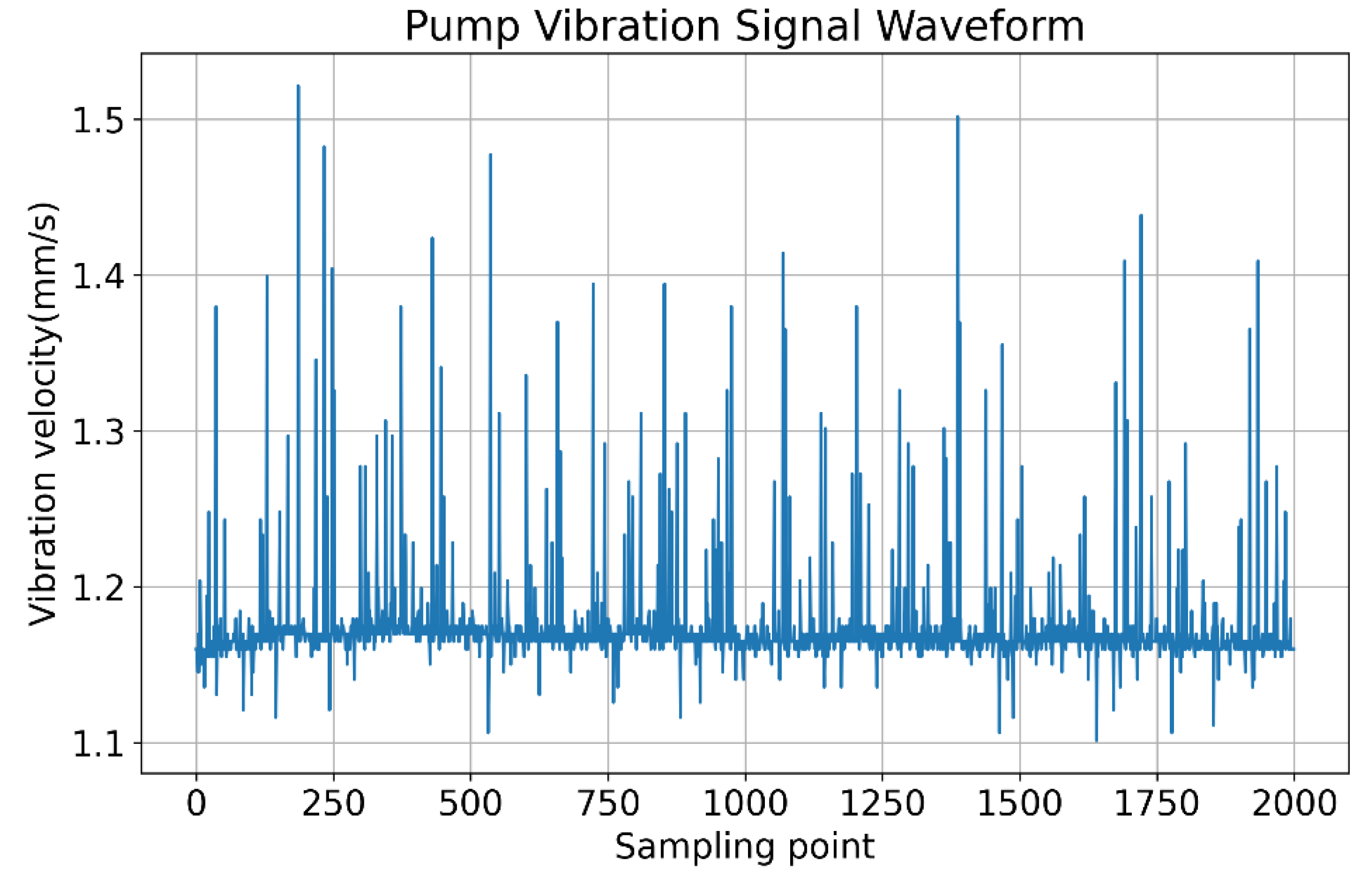
In Figure 3 below, the waveform diagram of the raw vibration signal data collected has the sample number along the x-axis and vibration velocity on the y-axis.

Three types of water pump vibration signal data were designed in this experiment: normal, slightly faulty, and severely faulty. The vibration signal data of normal water pumps were relatively easy to obtain, while those of faulty water pumps have been generated by manually disassembling and modifying the bearing parts. Specifically, bearings of normal water pumps were removed and subjected to chemical corrosion. The slightly and severely faulty types were defined according to their exposure time to corrosion (duration). The water pump vibration signal data read by the acquisition card were stored in an Excel file. In this way, we collected nine sets each of normal data, slightly faulty data, and severely faulty data (

Table 4. Experimental collection of the vibration signal dataset.

Type	Bearing Corrosion Duration (h)	Number of Groups	Sampling Points	Sample Number of Time–frequency Diagram
Normal	0	9	460,800	1791
Minor fault	3	9	460,800	1791
Serious fault	9	9	460,800	1791

). The sampling frequency was fixed at 10 kHz, with 51,200 single-sampling points, and a total of 1,382,400 pieces of experimental data, evenly split among the three types (Table 4).

2.4. Data Preprocessing

To improve model performance and accelerate algorithm convergence, the water pump vibration signal data were first normalized using Equation (1).

$$x_i^{\prime }={\displaystyle \frac{x_i-x_{min}}{x_{max}-x_{min}}}$$

(1)

In the above formula, $x_i$ denotes the feature value of the i-th sample in the dataset; $x_{min}$ and $x_{max}$ are, respectively, the minimum and maximum value among the samples in the dataset; and $x_i^{\prime }$ is the normalized feature value, whose range is [0, 1]. To prevent the overfitting of the model during its training due to a small number of samples, we used the overlapping sampling method to augment the number of samples [21], for which the sample step size was 512, and the overlap rate was set to 0.5.

After resampling, the dataset was split into a training set, validation set, and test set in a ratio of 7:2:1. Next, we formatted the dataset as required by the model, with data saved in a temporary file for subsequent model training.

2.5. Model-Building Steps

Here, we elaborate on each module of the model in detail:

(1)

Conversion of one-dimensional vibration signals into two-dimensional time–frequency diagrams. When a water pump malfunctions, for example, due to bearing corrosion or wear, its vibration signals are shaped by multiple factors including the pump itself and the surrounding aquatic environment. These signals are characterized by both nonlinearity and nonstationarity. Compared with previous analysis methods that independently analyze the time domain or the frequency domain, an analytical method that merges these two domains can extract critical features more effectively [22,23]. The continuous wavelet transform (CWT) can perform local transformations in space and time, and can efficiently extract key information from signals [24,25]. So, the CWT was selected here to convert the water pump vibration data into time–frequency images, using Equation (2).

$$CWT\left(a,b\right)={\displaystyle \frac{1}{\sqrt{a}}}{\int }_{-\infty }^{+\infty }x\left(t\right)\phi \left({\displaystyle \frac{t-b}{a}}\right)dt$$

(2)

In the above formula for CWT, $x\left(t\right)$ is the input data; a is the scale parameter; b is the translation parameter; and φ is the wavelet basis function. The CWT’s parameters were set as follows: sampling period = 1/12,000, total scale = 128, and wavelet basis function = ‘cmor1-1’.

(2)

The time–frequency image data are inputted into the CNN. After passing through the convolutional activation layer, the maximum pooling layer, the convolutional activation layer, and the maximum pooling layer again [26,27], the output data are finally used as the input for the next module in the model.

(3)

The output data of the previous module serve as input of this module. The transformer mainly consists of two parts: an encoder and a decoder, which may be used separately according to a given task’s requirements. In this paper, only the encoder part was actually used. It contains a multi-head self-attention mechanism and a feed-forward neural network. Residual connections and layer normalization are used to process the output of each sub-layer to enhance model training and convergence [28]. Finally, the output result is designated as input for use in the next module.

(4)

The output data of the previous module act as input for the BiGRU module. The model is improved upon by changing the GRU into a two-directional one. The forward GRU processes the data from the start of a sequence to its end, fully capturing its forward information; conversely, the backward GRU processes the data from the end of the sequence to its start, thus capturing its reverse information. This BiGRU is a powerful sequence data processing model. Through its bidirectional structure and gating mechanism, it can effectively capture the context information of the sequence and overcome the problem of gradient disappearance [29,30,31].

Finally, in classification problems, the fully connected layer is often used as the last layer of the neural network, and the number of its output nodes is usually equal to the number of classification categories. After completing the feature extraction and transformation of each previous layer, the fully connected layer calculates the score of each category according to the input features. Next, the Softmax function converts these scores into a probability distribution. By determining the magnitude of each probability value, the category with the maximum probability value is selected to determine the specific classification of the input sample.

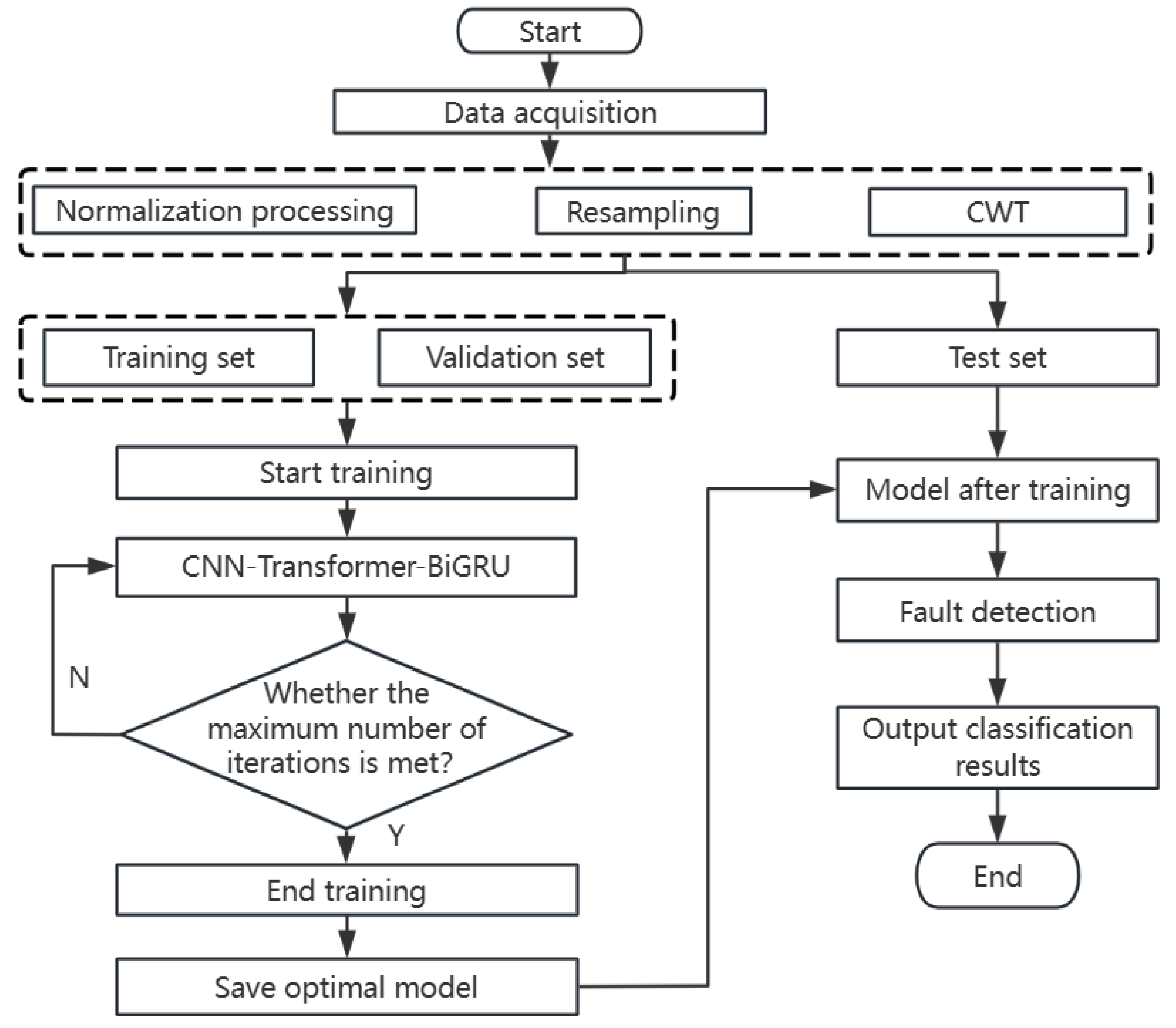
2.6. Fault Detection Process

The water pump fault detection process is divided into five phases: data collection, data preprocessing, model selection and construction, model training (iterative training to save the optimal model), and use of the optimal model for fault detection. This entire process is sketched in Figure 4.

3. Experiments and Results

3.1. Experimental Environment

This paper’s overarching aim was to evaluate the performance of the CNN-transformer-BiGRU for the task of fault detection in water pumps in IRASs. To ensure the accuracy and reliability of the experimental data and render them reproducible, this work was carried out in an environment with the specific hardware and software parameters listed in

Table 5. The experimental environment’s parameters.

Parameter Name	Value or Item
Operating system	Windows 11
Processor model	11th Gen Intel(R) Core(TM) i9-11900K @ 3.5 GHz
Memory capacity	64 GB
Graphics card Model	NVIDIA GeForce RTX 3080 Ti
Video Memory capacity	12 GB
Python	3.8.3.final.0
Pytorch	2.3.0 + cu118
CUDA version	12.6

.

To train the model faster, we chose to use an NVIDIA GeForce RTX 3080 Ti graphics card with a dedicated 12 GB GPU memory. It supports Cuda parallel computing, which can significantly improve the computational speed of operations, such as convolutional calculations and matrix multiplications [32]. The experimental algorithm model was developed using Python, and the network framework is Pytorch.

3.2. Model Parameter Adjustment

To analyze how different hyperparameters affect the model’s performance, in this study, we employed the controlled variable method and conducted multiple rounds of experimental comparisons by setting different model parameters based on empirical tuning. That is, only one hyperparameter is changed each time, while all others are left unchanged, to accurately determine the given impact of a single variable on the model. Four different models were selected for this experiment, the results of which are presented in Figure 5.

The stochastic gradient descent (SGD) can be used to iteratively update the model’s parameters, but it is evidently prone to instability in the convergence process, with large fluctuations in its curve. The average stochastic gradient descent (ASGD) improves upon the SGD, by introducing the idea of parameter averaging, which also enhances convergence stability. Adaptive Moment Estimation (Adam) can adaptively adjust the learning rate and combines the advantages of the AdaGrad and RMSProp algorithms [33]. Compared with SGD, it converges faster and has an improved stability, but it is prone to the problem of decay. AdamW is an improvement to the Adam algorithm and is mainly used to solve the latter’s occasional weight decay problem [34]. In comparing the experimental results, we found that AdamW had the best convergence speed and stability.

A comparative experiment was then performed, by setting different parameter values for the learning rate and batch size. The learning rates were set to 1 × 10⁻³, 1 × 10⁻⁴, or 1 × 10⁻⁵, respectively, and the batch sizes to 16, 32, or 64, in combination. These results are shown in Figure 6.

The batch size plays a crucial role in model training, because it determines the number of samples inputted to the model in each time step. If the batch size is set too large, the model is quite likely to fall into the dilemma of local optimality during training, consequently affecting its performance. Conversely, when the batch size is set too small, while this helps the model escape from local optimality, the training efficiency is significantly reduced, thereby incurring more time costs. The learning rate governs the step size of model parameter updates. If that value is set too high, the model is apt to skip the optimal solution due to overly large step sizes when updating parameters, and ultimately fails to converge; however, if set too small, the magnitude of each parameter update of the model could be minimal, greatly prolonging the training time required. Therefore, given the results (Figure 6), the best combination of parameters to use was a batch size of 32 and a learning rate of 1 × 10⁻⁴.

Similarly, another experiment was carried out, in which different parameter values were tested for the size of the convolutional kernel and the number of convolutional kernels. The former was set to 2 × 2, 3 × 3, or 4 × 4 and the latter to 32, 64, or 128, in combination. These results are shown in Figure 7.

This revealed a certain association between the size of the convolutional kernel and the accuracy of the model. As the former gradually increases, the latter does not change linearly. Instead, it first rose, reached a certain peak, and then fell. In the initial stage, a larger convolutional kernel could capture more abundant feature information. Nevertheless, when the size of the convolutional kernel exceeds a reasonable range, the feature extraction efficiency of the model will decrease, so it is likely to miss local key features, increasing the risk of overfitting and causing its accuracy to decline. Likewise, in adjusting the number of convolutional kernels and observing their impact on model accuracy, a similar hump-shaped pattern emerged. The model’s accuracy increases at first and then decreases with more convolutional kernels. This result may be attributed to the number of convolutional kernels exceeding a threshold, after which the model complexity becomes too high, with the training data not expanding sufficiently in tandem. Without more training data, it is challenging to properly support the training and learning of a highly complex model, so overfitting becomes more likely, causing the model’s accuracy to decline. Accordingly, based on the Figure 7 results, the best combination of parameters to select was 3 × 3 and 64 for the size and number of convolutional kernels, respectively.

3.3. Experimental Parameters

After multiple rounds of parameter optimization and adjustment, by comparing the model’s performance after each parameter adjustment, its optimal parameters were gleaned and saved for later use as the experimental parameters. These model parameters are listed in

Table 6. Experimental model parameters used in this paper.

Parameter Name	Value
Optimizer	AdamW
Learning rate	1 × 10−4
Convolution kernel size	3 × 3
Number of convolution kernels	64
Encoder layers	2
Number of multiple heads of attention	4
Attention dimension	128
Dropout	0.5
Batch size	32
Epochs	50

.

3.4. Model Training

Model training is a process where the model learns patterns and rules from data. First, the preprocessed training data are provided as input into the model to initiate the forward propagation process. Based on the input data and internal parameters, corresponding prediction results are then calculated. Following that, a loss function is introduced to calculate the loss value according to the difference between the prediction results and the true labels. Next, using the back-propagation mechanism, the gradients are calculated in reverse along each layer of the model’s structure. Then, an optimization algorithm is finally used to update the model parameters in a timely manner according to the calculated gradients, enabling the model to gradually approach the optimal state. After multiple rounds of iteration, the optimal model was obtained to achieve accurate prediction or classification of the data.

The model was trained using the above parameters, as seen in its curves for accuracy and loss values (Figure 8).

After 30 rounds of training, it started to stabilize. By comparing Figure 5, it can be concluded that the optimization strategy of AdamW was selected for model training, which accelerates model convergence and reduces significant fluctuations in the loss curve. By comparing Figure 6, it can be seen that setting the batch processing parameter to 32 and the learning rate to 1 × 10⁻⁴ during model training reduces the risk of underfitting and overfitting, while also improving model training efficiency.

The confusion matrix of the classification results can be seen in Figure 9 below.

The confusion matrix intuitively and clearly demonstrates the differences between true and predicted labels, as well as the classification results of each category, indicating that the model has a high classification capability. The number of correct identifications for severe fault types is 174, suggesting that the model performs best in identifying severe fault categories. However, the number of minor fault types misidentified as normal water pumps is 20, indicating that the model’s diagnostic capability between minor faults and normal conditions requires improvement.

3.5. Evaluating Indicator

This study adopted the commonly used evaluation metrics for classification tasks, namely accuracy (Acc), precision (P), recall (R), and the harmonic mean F1 of precision and recall. Their specific formulas are given in Equations (3)–(6).

$$Acc={\displaystyle \frac{TP+TN}{TP+TN+FN+FP}}$$

(3)

$$P={\displaystyle \frac{TP}{TP+FP}}$$

(4)

$$R={\displaystyle \frac{TP}{TP+FN}}$$

(5)

$$F1=2{\displaystyle \frac{P\ast R}{P+R}}$$

(6)

In the above formulas, TP denotes true positives, TN denotes true negatives, FP denotes false positives, and FN denotes false negatives. For multi-class classification tasks, such as the three-class classification situation in this model, the macro-average method was adopted. First, the metrics (such as precision and recall) are calculated for each class independently, and then, the arithmetic mean of these metrics was computed. The macro-average calculation formulas for precision and recall are shown in Equations (7) and (8).

$$macro-P={\displaystyle \frac{1}{C}}{\sum }_{i=1}^C{\displaystyle \frac{TP}{TP+FP}}$$

(7)

$$macro-R={\displaystyle \frac{1}{C}}{\sum }_{i=1}^C{\displaystyle \frac{TP}{TP+FN}}$$

(8)

3.6. Comparative Experiment

To verify the performance and feasibility of this paper’s proposed model in the task of fault detection for water pumps in IRASs, another experiment was conducted. This compared the performance of our model vis-à-vis a suite of commonly used models in the vibration signal classification task: KNN, SVM, random forest, LSTM, BiLSTM, KAN-GRU, Swin-transformer, CNN-attention, and CNN-LSTM. These comparative results are presented in

Table 7. Results for the accuracy (Acc), precision (P), and recall (R) of different tested models.

Model	Acc (%)	P (%)	R (%)
KNN	75.05	75.16	75.05
Random Forest	80.63	80.63	80.63
SVM	82.87	82.90	82.87
LSTM	85.10	85.31	85.10
BiLSTM	87.34	87.36	87.34
Swin-Transformer	87.15	87.14	87.15
KAN-GRU	88.83	88.81	88.83
CNN-Attention	84.54	84.70	84.54
CNN-LSTM	89.57	89.55	89.57
CNN-Transformer-BiGRU	91.43	91.52	91.43

Note: Acc, accuracy; P, precision; R, recall.

.

3.7. Ablation Experiment

Lastly, to verify the effectiveness of the improvements made in this paper for the task of water pump fault detection, a module ablation experiment was conducted. The CNN module, the transformer module, and BiGRU module were removed, respectively, and then the training and testing were carried out. These results are presented in

Table 8. Results for the accuracy (Acc), precision (P), and recall (R) of the ablation experiment.

Model	Acc (%)	P (%)	R (%)
CNN-Transformer-BiGRU	91.43	91.52	91.43
BiGRU	88.64	88.76	88.64
Transformer	87.15	87.37	87.15
CNN	83.24	83.56	83.24

Note: Acc, accuracy; P, precision; R, recall.

.

4. Discussion

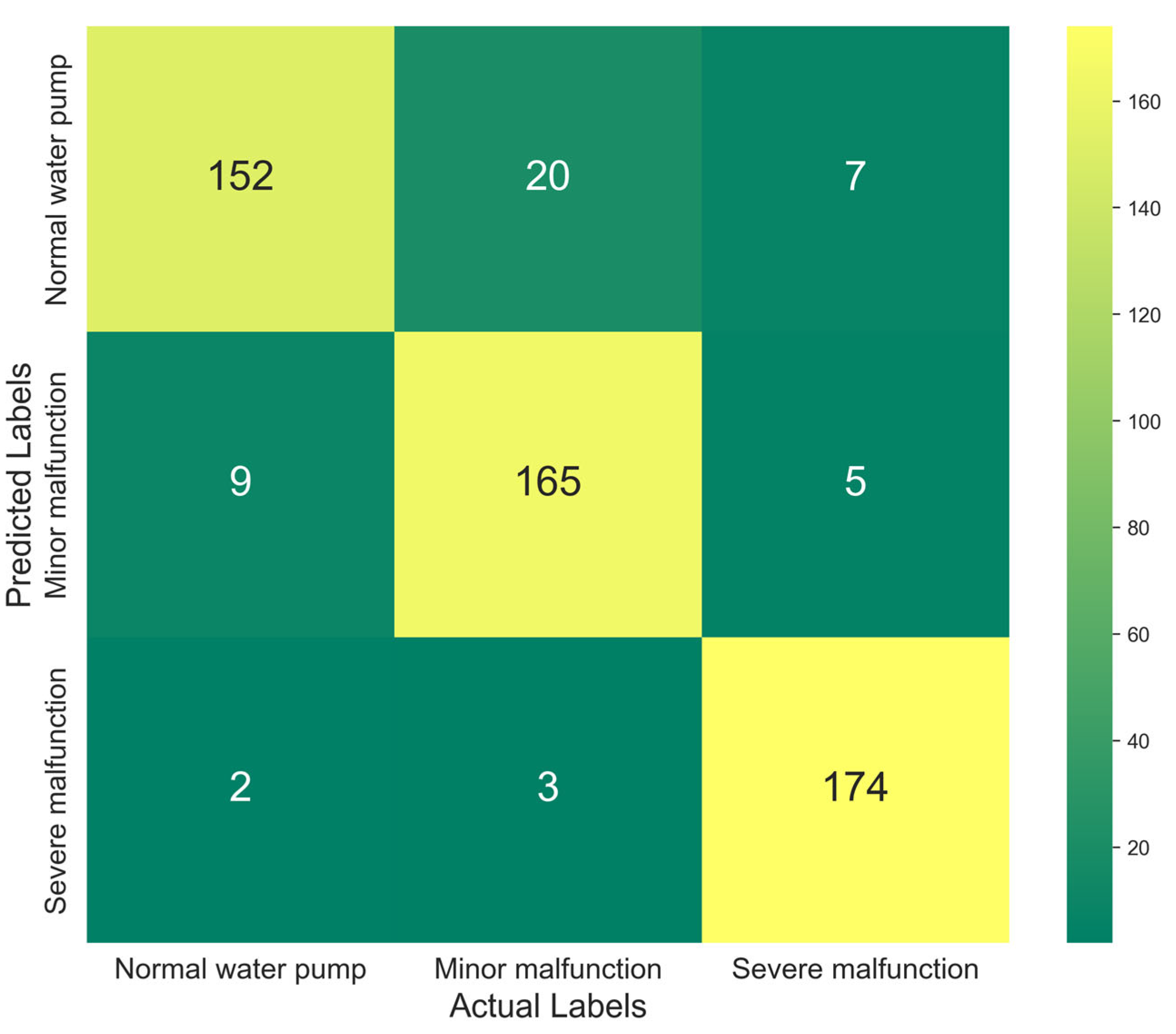
This comprehensive modeling study confirms that the vibration signals of water pumps can be used to quantitatively evaluate their operating status and the degree of faults they may incur. This paper proposed a method based on a deep learning model to objectively detect and identify such faults, and this model is applied in the field of recirculating aquaculture for the first time. Data from normal operation, minor faults, and serious faults were, respectively, collected to train and test the model, so as to determine the three working condition types of the water pump. The experimental classification results are conveyed in Figure 9, indicating the new model can effectively identify the water pump’s working condition types. This demonstrates that the water pump fault detection method based on the CNN-transformer-BiGRU model is effective.

To verify the performance and superiority of the model, nine different model validations were carried out and compared (Table 7). It can be seen that the traditional machine learning algorithms, such as the support vector machine (SVM), random forest (RF), and K-nearest neighbors (KNN), perform poorly at the task at hand, likely because the vibration signal data of water pump faults are affected by an array of complex factors, and those algorithms struggle to manually extract the appropriate characteristic information, such as margin factors, pulse factors, and peak-to-peak values [35,36]. The model proposed in this paper achieved robust performance when applied to the dataset of water pump faults in industrial recirculating aquaculture systems. The results for the test set are consistent with the F1 value curve of the validation set. Compared with the CNN-LSTM, the model in this paper leverages the advantages of the self-attention mechanism and demonstrates better performance. When compared with the Swin-transformer, the model highlights the advantages of the convolutional module in capturing features from time–frequency feature maps. Through experimental tests, we find that several network models, including BiLSTM, KAN-GRU, and CNN-LSTM, attain relatively high accuracy rates. But when these are directly compared with our proposed model, a performance gap persists.

Importantly, ablation experiments were also conducted in this study. To conduct these experiments, some of the model’s modules were removed for experiments, whose results are compared in Table 8. This clearly shows that removing the CNN led to a significant decline in all indicators of the entire model. The Acc, P, R, and F1 indicators were, respectively, reduced by 8.19%, 7.96%, 8.19%, and 8.07%. From this, we may infer that by converting the complex one-dimensional vibration signals into two-dimensional time–frequency images and then applying the CNN’s powerful processing ability to the latter, the fault characteristic information can be efficiently extracted [37,38]. Hence, the absence of this module has the greatest impact on model performance. After removing the transformer or BiGRU module, all indicators more or less decreased; this suggests that the encoder in the transformer improves the model’s hierarchical learning ability for features, and the self-attention mechanism strengthens the weights of the key features of the vibration signals. The BiGRU module is capable of more comprehensively capturing the front and back characteristic information in the vibration signal sequence, further enhancing the overall performance of the model [39].

In actual aquaculture settings, the characteristic signals indicating water pump faults may include distinctive signal features such as vibration, current, and sound. The research content of this paper is limited to vibration signal data and does not involve experiments on other signal data such as current and sound. The actual aquaculture environment is complex, with issues such as multiple interferences. Therefore, future research should focus on fusing multiple signal features, ideally according to a certain weight ratio, and then use these fused signals in model training. Pursuing this approach will enhance the robustness and universality of the introduced model in real-world environments and applications.

5. Conclusions

This paper strove to solve three core problems in the fault detection of water pumps in IRASs. (1) When the equipment has a minor fault, it can still operate normally, but the external manifestations of that fault are inconspicuous. The early prediction of the fault is crucial, and timely warnings for equipment maintenance and upkeep should be provided. (2) The vibration signals are complex and nonlinear, being easily influenced by multiple factors, such as background noise, the vibration of other equipment, and water flow. It is thus pivotal to extract information about the fault’s characteristic from both the time domain and frequency domain. (3) Whether the water pump has a minor or serious fault, a certain correlation exists in the vibration signals before and after, so it is necessary to handle the long-distance dependency in the sequence.

After conducting experiments on hyperparameter adjustment, comparison experiments with commonly used models for fault detection, followed by experimental removals of various modules in the model itself, these results were compared and synthesized with multiple indicators, such as accuracy and precision, for model evaluation. The accuracy of the model proposed here is 91.43%, this being significantly better than that of comparable models.

As such, this paper’s CNN-transformer-BiGRU model can effectively solve the above three problems and meet the performance requirements of the fault detection task in aquaculture and agriculture at large.

In the future, this model will incorporate signal data such as current and sound to improve multi-sensor data fusion, thereby enhancing the model’s diagnostic performance under complex working conditions.

References

1. Feng, T.; Chen, K.D. Discussion on Intelligent Control Technology for High-Efficiency Industrial Aquaculture in Ecological Recirculating Water. South. Agric. 2025, 19, 146–148. [Google Scholar]
2. Zhu, M.; Tan, H.Q.; Niu, Z.Y.; Wan, P.; Feng, Y.Z.; Li, L.; Huang, H.; Han, Y.H. Research on the Transformation and Upgrading Path of Freshwater Fisheries and the Key Points of Engineering Science and Technology Innovation in China. J. Huazhong Agric. Univ. 2024, 43, 1–9. [Google Scholar]
3. Cressey, D. Future Fish. Nature 2009, 458, 398–400. [Google Scholar] [CrossRef] [PubMed]
4. Jaap, V.R. Waste Treatment in Recirculating Aquaculture Systems. Aquacult. Eng. 2013, 53, 49–56. [Google Scholar]
5. Zan, T.; Pang, Z.L.; Wang, M.; Gao, X.S. An Early Fault Diagnosis Method for Rolling Bearings Based on Variational Mode Decomposition. J. Beijing Univ. Technol. 2019, 45, 103–110. [Google Scholar]
6. Lv, F.X.; Miao, Y.; Bie, F.F.; Peng, J.; Li, R.R. Application Research of ICEEMDAN and GS-SVM Algorithms in Acoustic Emission Fault Diagnosis of Rolling Bearings. Noise Vib. Control 2022, 42, 92–97. [Google Scholar]
7. Hou, S.S.; Zheng, J.D.; Pan, H.Y.; Feng, K.; Liu, Q.Y.; Ni, Q. Multivariate Multi-Scale Cross-Fuzzy Entropy and SSA-SVM-Based Fault Diagnosis Method of Gearbox. Meas. Sci. Technol. 2024, 35, 056102. [Google Scholar] [CrossRef]
8. Li, Y.Y.; Yuan, M.; Wang, Y.; Cheng, A.Y. Fault Diagnosis of Motor Bearings Combining SVM and PSO. J. Chongqing Univ. 2018, 41, 99–107. [Google Scholar]
9. Wang, Q.F.; Yin, Z.D.; Tao, E. Research on Fault Diagnosis of V2G Charging Piles Based on Random Forest Algorithm. Electr. Meas. Instrum. 2024, 61, 111–118. [Google Scholar]
10. Yang, M.X.; Yu, Y.X.; Li, Q.; Qiu, X.B.; Xu, K.W. Bearing Monitoring and Fault Diagnosis of Hydraulic Turbine Units Based on KNN. Autom. Instrum. 2023, 4, 66–70. [Google Scholar]
11. Lu, D.L.; Ning, Q.; Yang, X.M. Fault Diagnosis of Rolling Bearings Using the KNN-Naive Bayes Algorithm. Comput. Meas. Control 2018, 26, 21–23. [Google Scholar]
12. Kumar, A.; Parey, A.; Kankar, P.K. A New Hybrid LSTM-GRU Model for Fault Diagnosis of Polymer Gears Using Vibration Signals. J. Vib. Eng. Technol. 2023, 12, 2729–2741. [Google Scholar] [CrossRef]
13. Jiang, H.G.; Zhu, M.; Jiang, X.Q. Equipment Fault Diagnosis Method Based on Knowledge Graph and Multi-Task Learning. J. Comput. Appl. 2024, 44, 72–78. [Google Scholar]
14. Ma, K.F.; Yao, H.C.; Ren, Z.Q.; Jia, Y.T.; Yu, F.Y. Fault Diagnosis Method for Automation Equipment in Smart Substations Based on AM-GRU. Electr. Eng. 2024, 19, 1–4. [Google Scholar]
15. Hao, S.; Ge, F.; Li, Y.; Jiang, J. Multisensor Bearing Fault Diagnosis Based on One-Dimensional Convolutional Long Short-Term Memory Networks. Measurement 2020, 159, 107802. [Google Scholar] [CrossRef]
16. Wang, M.; Li, J.; Xue, Y. A New Defect Diagnosis Method for Wire Rope Based on CNN-Transformer and Transfer Learning. Appl. Sci. 2023, 13, 7069. [Google Scholar] [CrossRef]
17. Cao, K.; Zhang, T.; Huang, J. Advanced hybrid LSTM-transformer architecture for real-time multi-task prediction in engineering systems. Sci. Rep. 2024, 14, 4890. [Google Scholar] [CrossRef]
18. Li, T.; Zhao, Z.; Sun, C.; Yan, R.; Chen, X. Multireceptive Field Graph Convolutional Networks for Machine Fault Diagnosis. IEEE Trans. Ind. Electron. 2020, 68, 12739–12749. [Google Scholar] [CrossRef]
19. Tian, Y.; Chen, Y.J.; Zhang, L.; Chen, L. A Bearing Fault Diagnosis Method Combining Frequency Domain Feature Extraction with a Dual-Stream CNN. Noise Vib. Control 2024, 44, 167–173. [Google Scholar]
20. Mo, C.; Huang, K.; Ji, H. A Lightweight and Precision Dual Track 1D and 2D Feature Fusion Convolutional Network for Machinery Equipment Fault Diagnosis. Sci. Rep. 2024, 14, 31666. [Google Scholar] [CrossRef]
21. Sasada, T.; Liu, Z.; Baba, T.; Hatano, K.; Kimura, Y. A Resampling Method for Imbalanced Datasets Considering Noise and Overlap. Procedia Comput. Sci. 2020, 176, 420–429. [Google Scholar] [CrossRef]
22. Wang, N.; Du, W.; Liu, H.; Zhang, K.; Li, Y.; He, Y.; Han, Z. Fine-Grained Leakage Detection for Water Supply Pipelines Based on CNN and Selective State-Space Models. Water 2025, 17, 1115. [Google Scholar] [CrossRef]
23. Han, K.; Wang, W.; Guo, J. Research on a Bearing Fault Diagnosis Method Based on a CNN-LSTM-GRU Model. Machines 2024, 12, 927. [Google Scholar] [CrossRef]
24. Zou, Y.; Liu, T.; Zhang, X. A Three-Channel Feature Fusion Approach Using Symmetric ResNet-BiLSTM Model for Bearing Fault Diagnosis. Symmetry 2025, 17, 427. [Google Scholar] [CrossRef]
25. Wang, C.; Feng, L.; Hou, S.; Ren, G.; Lu, T. A High-Impedance Fault Detection Method for Active Distribution Networks Based on Time–Frequency–Space Domain Fusion Features and Hybrid Convolutional Neural Network. Processes 2024, 12, 2712. [Google Scholar] [CrossRef]
26. Zhang, S.; Zhou, J.; Ma, X.; Pirttikangas, S.; Yang, C. TSViT: A Time Series Vision Transformer for Fault Diagnosis of Rotating Machinery. Appl. Sci. 2024, 14, 10781. [Google Scholar] [CrossRef]
27. Gao, J.; Guo, J.; Yuan, F.; Yi, T.; Zhang, F.; Shi, Y.; Li, Z.; Ke, Y.; Meng, Y. An Exploration into the Fault Diagnosis of Analog Circuits Using Enhanced Golden Eagle Optimized 1D-Convolutional Neural Network (CNN) with a Time-Frequency Domain Input and Attention Mechanism. Sensors 2024, 24, 390. [Google Scholar] [CrossRef]
28. Hou, Q.; Gao, Z.; Lu, M.; Yu, Y. A Hybrid Transformer-CNN Model for Interpolating Meteorological Data on the Tibetan Plateau. Atmosphere 2025, 16, 431. [Google Scholar] [CrossRef]
29. Xu, Z.; Li, Y.F.; Huang, H.Z.; Deng, Z.; Huang, Z. A Novel Method Based on CNN-BiGRU and AM Model for Bearing Fault Diagnosis. J. Mech. Sci. Technol. 2024, 38, 3361–3369. [Google Scholar] [CrossRef]
30. Amiri, A.F.; Kichou, S.; Oudira, H.; Chouder, A.; Silvestre, S. Fault Detection and Diagnosis of a Photovoltaic System Based on Deep Learning Using the Combination of a Convolutional Neural Network (CNN) and Bidirectional Gated Recurrent Unit (Bi-GRU). Sustainability 2024, 16, 1012. [Google Scholar] [CrossRef]
31. Wang, Y.; Zheng, D.; Jia, R. Fault Diagnosis Method for MMC-HVDC Based on Bi-GRU Neural Network. Energies 2022, 15, 994. [Google Scholar] [CrossRef]
32. Rao, D.; Ramana, K. Accelerating Training of Deep Neural Networks on GPU using CUDA. Int. J. Intell. Syst. Appl. 2019, 11, 9. [Google Scholar] [CrossRef]
33. Zhou, P.; Xie, X.Y.; Lin, Z.C.; Yan, S.C. Towards Understanding Convergence and Generalization of AdamW. IEEE Trans. Pattern Anal. Mach. Intell. 2024, 46, 6486–6493. [Google Scholar] [CrossRef] [PubMed]
34. Jiang, G. Security Detection Design for Laboratory Networks Based on Enhanced LSTM and AdamW Algorithms. Int. J. Inf. Technol. Syst. Approach 2023, 16, 1–13. [Google Scholar] [CrossRef]
35. Singh, S.; Kumar, N. Detection of Bearing Faults in Mechanical Systems Using Stator Current Monitoring. IEEE Trans. Ind. Inform. 2017, 13, 1341–1349. [Google Scholar] [CrossRef]
36. Gupta, P.; Pradhan, M.K. Fault Detection Analysis in Rolling Element Bearing: A Review. Mater. Today Proc. 2017, 4, 2085–2094. [Google Scholar] [CrossRef]
37. Du, X.; Jia, W.; Yu, P.; Shi, Y.; Cheng, S. A Remaining Useful Life Prediction Method Based on Time–Frequency Images of the Mechanical Vibration Signals. Measurement 2022, 202, 111782. [Google Scholar] [CrossRef]
38. Xiao, R.; Zhang, Z.; Wu, Y.; Jiang, P.; Deng, J. Multi-scale Information Fusion Model for Feature Extraction of Converter Transformer Vibration Signal. Measurement 2021, 180, 109555. [Google Scholar] [CrossRef]
39. Wang, Y.; Pang, G.; Wang, T.; Cong, X.; Pan, W.; Fu, X.; Wang, X.; Xu, Z. Future Reference Evapotranspiration Trends in Shandong Province, China: Based on SAO-CNN-BiGRU-Attention and CMIP6. Agriculture 2024, 14, 1556. [Google Scholar] [CrossRef]
Figure 1. Schematic structure of the newly proposed CNN-transformer-BiGRU model to detect water pump faults in industrialized recirculating aquaculture systems.
Applsci 15 06114 g001
Figure 2. Continuous acquisition process diagram for Analog-to-Digital collection used in this paper.
Applsci 15 06114 g002
Figure 3. Wave diagram of raw vibration signal data obtained.
Applsci 15 06114 g003
Figure 4. Flowchart for the model fault detection process used in this paper.
Applsci 15 06114 g004
Figure 5. Model training loss curves for several different optimization algorithms.
Applsci 15 06114 g005
Figure 6. Results for the accuracy of different combinations of learning rates and batch sizes.
Applsci 15 06114 g006
Figure 7. Results for the accuracy of different combinations of convolution kernel sizes and numbers.
Applsci 15 06114 g007
Figure 8. Comparison of model accuracy and loss curves.
Applsci 15 06114 g008
Figure 9. Classification confusion matrix.
Applsci 15 06114 g009