Data-Aware Path Planning for Autonomous Vehicles Using Reinforcement Learning ^†

Abstract

This paper addresses the challenge of optimizing path planning for autonomous vehicles in urban environments by considering both traffic and bandwidth variability on the road. Traditional path planning methods are inadequate for the needs of interconnected vehicles that require significant real-time data transfer. We propose a reinforcement learning approach for path planning, formulated to use road traffic conditions and bandwidth availability. This approach optimizes routes by minimizing travel time while maximizing data transfer capability. We create a realistic simulation environment using GraphML, incorporating real-world map data and vehicle mobility patterns to evaluate the effectiveness of our approach. Through comprehensive testing against various baselines, our reinforcement learning model demonstrates the ability to adapt and find optimal paths that significantly outperform conventional strategies. These results emphasize the feasibility of using reinforcement learning for dynamic path optimization and highlight its potential to improve both the efficiency of travel and the reliability of data-driven decisions in autonomous vehicular networks.

1. Introduction

The transition of autonomous vehicles from theoretical concepts to everyday reality marks a significant milestone in urban development, promising to transform transportation systems and urban infrastructures alike. This is not merely an advancement in vehicle control and navigation; it is a shift in how vehicles interact with their environment, passengers, and each other. Each autonomous vehicle, essentially a supercomputer on wheels, is estimated to generate up to 4 terabytes of data per day [1]. As these data-intensive vehicles become increasingly interconnected, they face a dual challenge, navigating not just through physical traffic but through an invisible sea of information.

Autonomous vehicles are equipped with a suite of advanced features that promise to redefine the driving experience. These vehicles can detect and navigate around obstacles, adjust speed in response to traffic conditions, and plan routes in real-time to avoid congestion [2]. Moreover, autonomous vehicles have the potential to significantly improve road safety by reducing human error, which is the leading cause of traffic accidents [3]. These capabilities are made possible by a combination of hardware and software technologies, including LiDAR sensors, radar sensors, cameras, and sophisticated machine learning algorithms. This technological synergy allows vehicles to perceive their surroundings, make decisions, and learn from experience with a high degree of precision and consistency.

Furthermore, with the advancement of vehicle-to-vehicle and vehicle-to-infrastructure communications, vehicles can now share information with components such as cameras, traffic lights, and even other vehicles [4]. This opens up new possibilities for managing traffic flow and reducing congestion, which can lead to a more efficient use of road networks and lower travel times. It can also allow vehicles to interact with roadside units with dedicated computing resources to offload computing processes from vehicles and to perform real-time calibration functions while on the road [5]. As a result, vehicles are evolving beyond their traditional role as means of transportation; they generate, store, process, and transmit large amounts of data used to improve driver convenience and safety [6].

Building on these transformative advancements in vehicular technology and the emerging capabilities of autonomous vehicles, a significant challenge has emerged in data management and communication. The integration of these technologies not only enhances the vehicle’s ability to navigate complex urban environments but also forms part of a larger, interconnected intelligent transportation system. This integration necessitates robust data management and transmission capabilities to fully utilize its potential. Furthermore, the introduction of 5G cellular networks, which aims to increase bandwidth for road data transmission, introduces additional challenges. The variability of these networks—affected by line of sight, infrastructure differences, and traffic density—can lead to fluctuations in data transmission rates and reliability.

This paper addresses the problem of path planning for autonomous vehicles within urban environments, where the need for timely data transfer is as important as minimizing driving time. We formulate the problem of path planning considering both traffic and bandwidth heterogeneity on the road as a reinforcement learning problem. To practically assess this formulation, we implemented an environment representing a graphical road network using GraphML [7]. This framework enables the incorporation of real map data and vehicle mobility patterns to create a realistic and robust testing ground to evaluate the reinforcement learning approach to path planning. Using real-world data, our model can simulate the dynamics of urban traffic, providing a comprehensive understanding of the challenges and opportunities in optimizing path planning for autonomous vehicles.

Through rigorous testing across various parameters, we demonstrate that our reinforcement learning approach can learn efficient and effective solutions. These solutions are shown to be superior to baseline models that do not account for the heterogeneity of traffic and bandwidth. Our findings indicate not only the viability of using reinforcement learning for this complex optimization problem but also its potential to significantly outperform traditional path planning methods.

The key contributions of this paper are as follows:

• A novel reinforcement learning framework that jointly optimizes for travel time and data transfer efficiency in heterogeneous urban environments.
• Implementation of a realistic simulation environment using GraphML [7], incorporating real map data and vehicle mobility patterns for robust evaluations of path planning strategies.
• Experimental validation demonstrating the superiority of our approach over traditional baselines in heterogeneous traffic and bandwidth scenarios.

The remainder of this paper is organized as follows: Section 2 presents a review of related work in the field. Section 3 details the core of our research, providing a comprehensive overview of the problem formulation. This section elaborates on the principles of reinforcement learning, details the construction of our reinforcement learning environment, and explains the experimental setup. In Section 4, we present and analyze the simulation results. Finally, Section 5 summarizes our findings and discusses their implications for the future of autonomous vehicle path planning.

2. Related Work

2.1. Path Planning

Path planning in autonomous vehicles is a critical component that ensures that these vehicles navigate from one point to another efficiently and safely. This process is broadly categorized into global and local path planning strategies [8]. Global path planning involves calculating a predefined route from the starting point to the destination based on high-precision maps that account for available road information, such as the length of the route and its traffic density. This method, often called static or offline planning, relies on comprehensive environmental data to determine the optimal geometric route without collisions [9]. On the other hand, local path planning, also known as dynamic or online planning, adapts to real-time environmental changes. It adjusts the vehicle’s trajectory in response to immediate obstacles or alterations in driving conditions, necessitating a flexible and responsive approach to path planning [9]. Path planning algorithms in autonomous vehicles rely on diverse search algorithms and are generally grouped into three categories, namely graph search algorithms, traditional algorithms, and group optimization algorithms [8].

Graph search algorithms such as Dijkstra’s algorithm are among the various algorithms used for path planning. Dijkstra’s algorithm is foundational, scanning all vertices within a distance smaller than the specified distance between the starting point and the destination. It provides a reliable but computationally intensive solution for finding routes in less complex environments [10]. The A* algorithm [11], a classic goal-directed shortest path algorithm, combines the Dijkstra algorithm with the Best First Search algorithm [12] and refines this approach by guiding the search toward the target more efficiently [8]. This method leverages the network’s geometric embeddings or the graph’s structural features, including the configuration of shortest path trees, to target compact areas [13]. However, its application in road networks that prioritize travel time as a metric can be limited due to its performance issues when geographic distance is used as a limit [14]. The D* (Dynamic A*) algorithm [15] represents a significant improvement in dynamic path planning, capable of adjusting the planned route in the face of obstacles, thus enhancing the efficiency of secondary path planning by reducing the exploration space and improving computational efficiency [16].

Many traditional algorithms are used for path planning, each catering to different navigational requirements and constraints. The artificial potential field (APF) algorithm creates a virtual force field around obstacles, repelling the autonomous agent away from obstacles and attracting it toward the target [17]. This method is intuitive and effective for simple environments, but it can be difficult to use in complex scenarios with local minima where the vehicle might get stuck. Simulated annealing [18] and Tabu search algorithms [19] offer sophisticated means of escaping local minima and finding globally optimal paths by intelligently exploring the search space.

The rapidly-exploring random tree (RRT) algorithm [20] stands out for its adaptability and efficiency in handling non-holonomic constraints, which are particularly relevant for autonomous vehicle navigation [21]. Holonomic systems are those in which the controllable degrees of freedom are equal to the total degrees of freedom, allowing for straightforward movement in any direction from any configuration [22]. This ideal scenario is not always practical in real-world navigation, especially for vehicles. Non-holonomic systems, in contrast, have constraints that limit the vehicle’s movement directions based on its current state [22]. For example, a car cannot move sideways and its turning radius imposes constraints on its path planning. The RRT algorithm excels in these environments by randomly sampling the space and incrementally building a tree of possible paths. This approach not only navigates around obstacles but also considers the vehicle’s physical capabilities and limitations, ensuring that the generated paths are feasible for non-holonomic agents [23]. Bast et al. [14] offer a detailed survey and comparison of practical algorithms designed for efficient path planning in both human-driven and autonomous vehicles. Energy-aware routing for electric vehicles has also been addressed with meta-heuristics; for example, Loaiza-Quintana et al. [24] apply an iterated local search algorithm to optimize e-bus charging-station placement, integrating battery constraints into route decisions.

Despite the utility of these algorithms, applying them to graph representations of large and complex road networks, especially when optimizing driving time, presents significant challenges. Classic shortest path algorithms like Dijkstra and A* become inefficient in handling road networks with millions of edges due to their computational demands [10,11,13]. Moreover, while RRT and other traditional algorithms offer solutions for non-holonomic cases and dynamic environments, their scalability and efficiency in large-scale, time-sensitive road network scenarios remain limiting factors.

2.2. Reinforcement Learning

Machine learning (ML) is a foundational domain within artificial intelligence (AI). It equips computers with the ability to learn and make decisions that mimic human intelligence [25]. This field is particularly renowned for its applications in signal processing and image processing [25,26,27], including significant advancements in speech recognition [28,29], natural language processing [30,31,32], and medical diagnostics [33,34].

At the heart of machine learning are three primary paradigms, namely supervised learning, where models make decisions based on previously provided output labels; unsupervised learning, which identifies patterns without prior output label knowledge; and reinforcement learning (RL), distinguished by its use of sequential actions to learn from interactions with the environment based on rewards or penalties [35].

RL is defined as a method by which an agent interacts with its environment to learn optimal behaviors without prior knowledge [36]. RL aims to maximize numerical rewards or minimize penalties. This interaction is facilitated by feedback on each action, allowing the agent to iteratively refine its policy to achieve the best possible control policy [35]. Figure 1 depicts this RL control loop. At each time step t, an agent follows an algorithm to observe the state of the system $s_t$, takes an action $a_t$, and receives a reward $r_t$. Based on its current policy, the agent’s action leads to a new state. With each interaction, the agent updates its understanding of the environment.

RL is a versatile and powerful technique with a broad range of applications, including task scheduling, game strategy development, image-based robot control, and path planning [37,38,39,40,41]. The actor–critic structure [42,43,44] and Q-learning [45,46,47,48] are frameworks in which RL can be implemented [36]. This diversity in approaches allows RL to effectively address complex decision-making and optimization problems across different domains.

Various network structures, including wireless sensor networks [49], vehicular ad hoc networks (VANETs) [50], flying ad hoc networks [51], and drone ad hoc networks [52], benefit from the application of RL algorithms to their routing algorithms [53]. VANETs present a unique application domain for RL. These networks, which facilitate communication between vehicles and road-side infrastructure, support a wide range of applications, from emergency alerts to road safety and information services [54,55,56,57,58]. High mobility and computational capabilities are characteristics of VANETs that make them an interesting subject for RL-based optimization [59]. In their work, Nazib et al. compared RL-based routing protocols, analyzing their mechanisms, advantages, disadvantages, and practical applications [53]. RL algorithms primarily focus on optimizing various quality-of-service metrics, including throughput, overhead, and end-to-end delay [60,61].

RL has shown promise within the field of autonomous vehicle motion planning. Solutions for planning challenges have been developed using artificial intelligence, including deep learning models for optimal control action learning and multi-robot navigation algorithms that consider dynamic obstacles [62,63,64,65,66].

Beyond these applications, the versatility of RL extends to a wide array of driving functionalities such as car following [67], lane keeping [68], driver assistance [69], lane merging [70], highway merging [71], braking [72], and active steering [73]. RL solutions for traffic signal control have also been shown to outperform standard control methods in simulation environments [74]. Each of these applications demonstrates the potential of RL not only to enhance navigational strategies and the driving performance of autonomous vehicles but also to contribute significantly to safety and efficiency in complex traffic scenarios.

Building on these foundations, several recent studies have explored the innovative applications of reinforcement learning to emerging vehicular challenges. Fei et al. [75] applied DRL to non-lane-based toll–plaza trajectories. Hussain et al. [76] and Sun et al. [77] explored RL-driven route optimization and energy-aware scheduling in IoV and logistics networks, respectively; Wang et al. [78] introduced a hybrid-state, risk-aware DRL decision model that improves maneuver safety in highway scenarios; Audinys et al. [79] leveraged vision transformer-based DRL for end-to-end visual self-driving control; and Lu et al. [80] proposed a hybrid DRL–kinematic autopilot framework that boosts decision reliability on motorways.

Although these works reflect the growing versatility of RL in autonomous driving, none of them jointly consider the role of wireless bandwidth maps in the decision-making process, leaving a critical research gap that our study addresses.

Our research identifies and addresses this gap by introducing a novel reinforcement learning framework for autonomous vehicle path planning that is explicitly aware of bandwidth heterogeneity. This approach is motivated by several factors, including the critical challenge of planning routes with adequate signal availability for connected autonomous vehicles. Recent research has highlighted users’ concerns when navigation systems suggest routes with poor signal coverage [81], underscoring the importance of this issue. Our work is distinctive in that it considers not only the traditional objectives of route planning, such as minimizing drive time and avoiding traffic, but also prioritizes high-bandwidth roads to meet the vehicle’s data transfer requirements. In doing so, our work fills a critical gap in the existing research, demonstrating the untapped potential of RL to improve the efficiency and efficacy of autonomous vehicles in urban environments with heterogeneous bandwidth conditions.

3. Problem Formulation

This paper explores the problem of path planning for autonomous vehicles within urban environments, where the need for timely data transfer is as important as minimizing drive time. Specifically, we assumed that each vehicle has a certain amount of data that must be successfully transferred before reaching its destination. In previous studies, this problem was explored and tested in a simple grid world environment [82]. To advance this exploration, we constructed a detailed and dynamic graphical representation of urban road networks, utilizing real-world vehicular mobility data to create a more realistic environment.

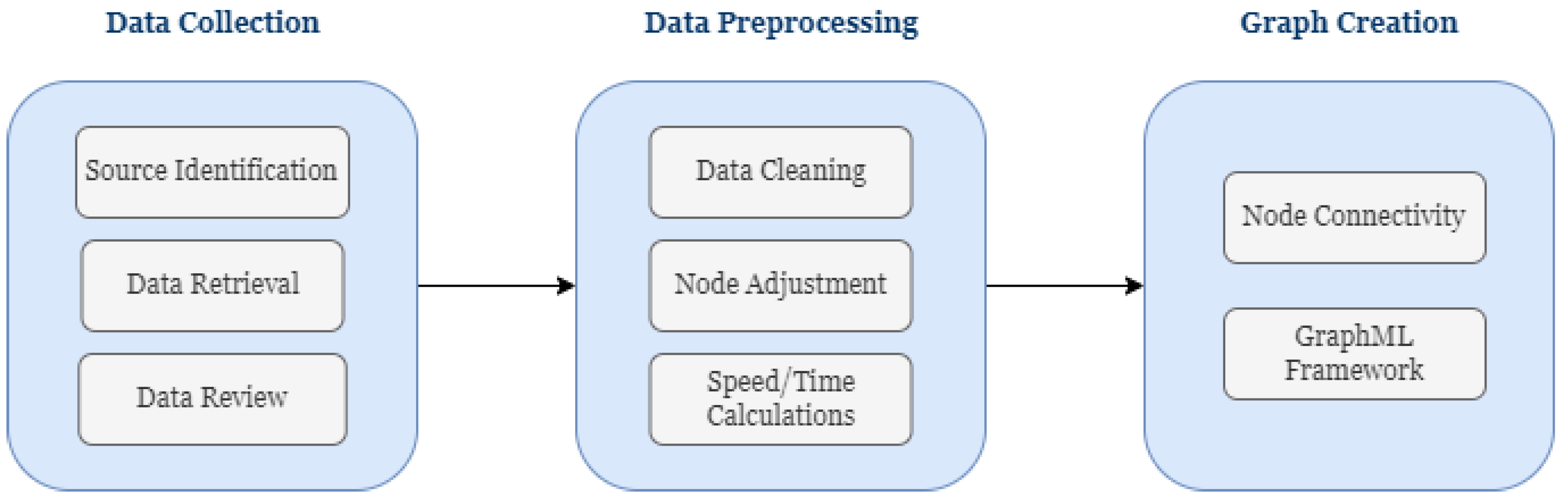
3.1. Constructing the Environment

We modeled the environment as a graphical road network, constructed using the GraphML framework. This model allows for the integration of real-world map data and vehicle mobility patterns, providing a realistic and dynamic setting for the evaluation of our RL-based path planning strategy. In this graphical network, roads are depicted as connections (edges) between nodes (intersections), where each node has a series of attributes. These include their precise coordinates, lengths of adjoining roads, the average duration vehicles occupy each road, vehicles’ average speed on each road, and a congestion factor that measures traffic density levels on each road.

Figure 2 illustrates the environment creation process. To achieve this, we used a vehicle mobility dataset (This dataset was obtained from the University of Southern California’s Autonomous Networks Research Group [https://anrg.usc.edu/www/downloads/ (accessed on 5 July 2023)]) consisting of time-stamped location coordinates of 3000 taxis in Beijing over a 24 h period. This dataset served as the basis for modeling this graphical road network.

We began preprocessing by extracting the full trajectory of each taxi and map-matching every GPS fix to OpenStreetMap using Valhalla (https://github.com/valhalla/valhalla (accessed on 13 November 2023)). For each vehicle, we recorded the sequence of visited nodes (intersections) and computed the distance, speed, and travel time between consecutive nodes. A point was tagged stationary when its instantaneous speed remained below 3 km/h for at least 60 s; such points, typically parking or long red light stops, were removed so that the analysis reflected only in-motion segments. Congestion factors were calculated as the ratio of observed-to-free-flow speed, aggregated in 10 min windows. Assuming bidirectional travel on all roads, we consolidated nodes that lay on the same heading (within ±5°) and were separated by less than 20 m, thereby reducing graph complexity without altering connectivity.

After preprocessing the user data in the dataset, we created a JSON file that recorded the number of edges connected to each node. This JSON file, together with the preprocessed data, was used to build a detailed representation of vehicle mobility patterns on roads using the GraphML framework. Figure 3 displays the entire graphical network, which represents not only the physical layout of the road network but also the dynamic factors such as traffic congestion and speed patterns. The top graph shows a birds-eye overview of the entire Beijing graph, confirming that the extracted topology matches the street grid. The bottom graph shows a zoomed-in portion of the map, highlighting node consolidation and edge connections after preprocessing. This graphical model forms the basis of our reinforcement learning environment, facilitating the training and testing of reinforcement learning algorithms under realistic traffic conditions.

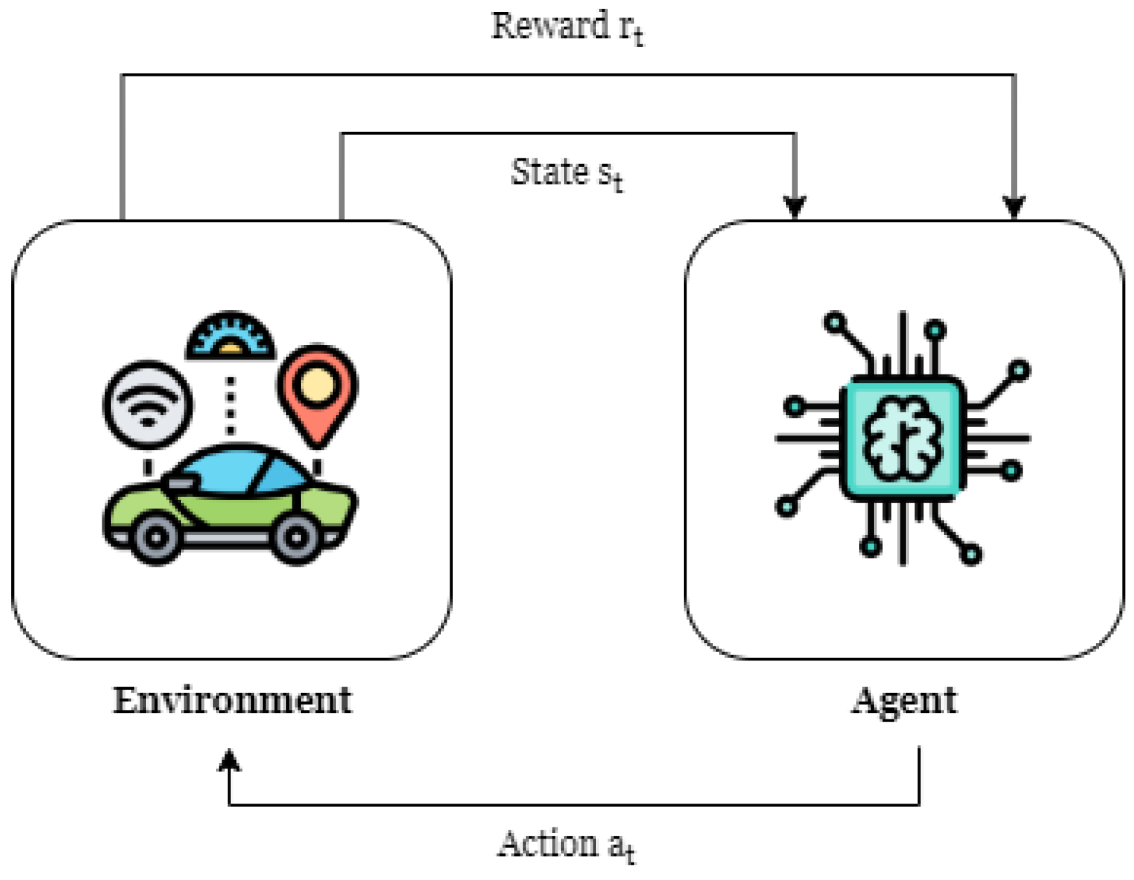
3.2. Reinforcement Learning Formulation

In our problem, each action retains and senses information about the environment’s state. This characteristic demonstrates the Markov property, allowing us to model our problem as a stochastic Markov Decision Process. At the start of each episode, we randomly sampled traffic congestion and wireless bandwidth fields from the empirical dataset; these fields then evolved according to the random fluctuations observed in the trace, so the agent experienced genuinely stochastic state transitions.

3.2.1. Goal

The goal of the agent was to transfer all its data while also reaching the destination as fast as possible.

3.2.2. State Space (S)

The state space S of our environment is defined by several key parameters that encapsulate both the physical position and the communication objectives of the agent.

$$S=\left\{\right(x,d,B,T)\mid x\in X,d\ge 0,B\in \mathcal{B},T\in \mathcal{T}\}$$

where

• x represents the current node position of the agent within the network.
• d is the remaining amount of data that needs to be transferred. This component reflects the agent’s communication objectives, crucial to ensuring that data transfer requirements are met before the journey ends.
• B denotes the set of bandwidths available on the links connected to the current node x. Each element in B represents the bandwidth on a specific link, which affects the rate at which data can be transferred as the agent considers its next move.
• T indicates the set of traffic densities on the links connected to the current node x. Each element in T reflects the traffic density on a specific link, which affects the agent’s travel time and decision-making for route optimization.

The bandwidth and traffic density vectors B and T are restricted to the links directly connected to the current node x; the agent therefore observes only its immediate neighboring nodes and not the entire network. The quantities B and T are observations that include zero-mean Gaussian noise to emulate sensing uncertainty and avoid the unrealistic assumption of perfect measurement.

Together, these parameters provide a multidimensional snapshot of the environment from which the agent can make its decisions.

3.2.3. Action Space (A)

The action space A of our reinforcement learning model is directly defined by the agent’s current node and the accessible links. It is structured as follows:

$$A\left(x\right)=\{x^{\prime }\mid (x,x^{\prime })\in L\}$$

where

• x represents the current node position of the agent.
• $x^{\prime }$ denotes a potential next node to which the agent can move.
• L is the set of all the connections in the network, where each link is a tuple $(x,x^{\prime })$ that indicates a direct connection from node x to node $x^{\prime }$.

This definition ensures that the action space is dynamically adjusted based on the agent’s current position, reflecting the physical and network connectivity constraints. The agent selects from the set of possible next nodes to which it can move based on the links available at its current node. This allows for a flexible yet precise mechanism to navigate through the network, making decisions that are optimal with respect to both route efficiency and data transmission needs.

3.2.4. Reward Function (R)

The reward function R of our reinforcement learning model is designed to align the agent’s actions with the dual objectives of fast route navigation and complete data transfer. The function is defined as follows:

$$R(s,a,s^{\prime })=\left\{\begin{array}{cc}{R}_{\mathrm{complete}}\hfill & \mathrm{if}{d}^{\prime }=0\mathrm{and}{x}^{\prime }=x_{\mathrm{dest}}\hfill \\ \alpha R_{\mathrm{travel}}(x,x^{\prime })+\beta R_{\mathrm{data}}(d,d^{\prime })-\gamma R_{\mathrm{punish}}(x,x^{\prime })\hfill & \mathrm{otherwise}\hfill \end{array}\right.$$

where

• $R_{\mathrm{complete}}$ is a large positive reward given when the agent reaches the destination $x_{\mathrm{dest}}$ with no remaining data to transfer ($d^{\prime }=0$).
• $R_{\mathrm{travel}}(x,x^{\prime })$ represents the fractional reward for traveling from node x to node $x^{\prime }$, designed to encourage faster routes. The amount of this reward inversely correlates with the travel time or distance traveled.
• $R_{\mathrm{data}}(d,d^{\prime })$ is the reward for data transferred during the transition from d to $d^{\prime }$, structured to incentivize maximum data transfer throughout the journey.
• $R_{\mathrm{punish}}(x,x^{\prime })$ encompasses penalties for inefficiencies, such as remaining stationary ($x=x^{\prime }$ and $d=d^{\prime }$), revisiting previously visited nodes, or selecting slower routes.

The scalar weights $\alpha ,\beta ,\gamma$ were chosen in two steps. We first expressed the value of a one-second travel delay and a 1 kbit data transfer in the same monetary units, which yielded $\alpha =\beta =1$. The inefficiency term should discourage route loops but not overwhelm the primary objectives, so we set $\gamma =0.2$ after a coarse grid check $\gamma \in \{0.1,0.2,0.3\}$ on the validation logs. Because our return is a potential-based positive sum of atomic rewards, any common scaling of $\alpha ,\beta ,\gamma$ leaves the optimal policy unchanged [83]. When $\alpha ,\beta$ were varied in $\{0.5,1,2\}$ and $\gamma$ in $\{0.1,0.2,0.3\}$, the mean episode return changed by less than 4%, showing that the policy is robust to reasonable re-weightings.

3.2.5. Transition Probability (P)

The transition probability quantifies the generally stochastic likelihood of transitioning from one state to another given an action; its variability is driven by the sampled congestion and bandwidth fields described above. It is defined mathematically as

$$P(S_{t+1}=s^{\prime }\mid S_t=s,A_t=a)$$

where

• $S_t$ denotes the current state at time t.
• $A_t$ represents the action taken at time t from state $S_t$.
• $S_{t+1}$ is the state at time $t+1$, resulting from taking action $A_t$ in state $S_t$.

3.2.6. Policy ($\pi$)

The policy determines the agent’s actions based on the current state of the environment. The policy is defined as a deterministic function that maps each state s from the state space S to a specific action a in the action space A.

In our model, the agent follows a deterministic policy $\pi$, defined by the following mapping:

$$\pi :S\to A$$

where

• $s\in S$ denotes the current state of the agent within the environment.
• $a=\pi \left(s\right)$ represents the action chosen by the policy.

The optimization of $\pi$ is achieved through iterative updates based on the outcomes of actions taken in various states. This iterative process refines the policy by learning from past experiences, thus improving the decision-making process over time. The effectiveness of the policy is measured by its ability to consistently achieve higher rewards and fulfill the agent’s objectives within the defined constraints of the environment.

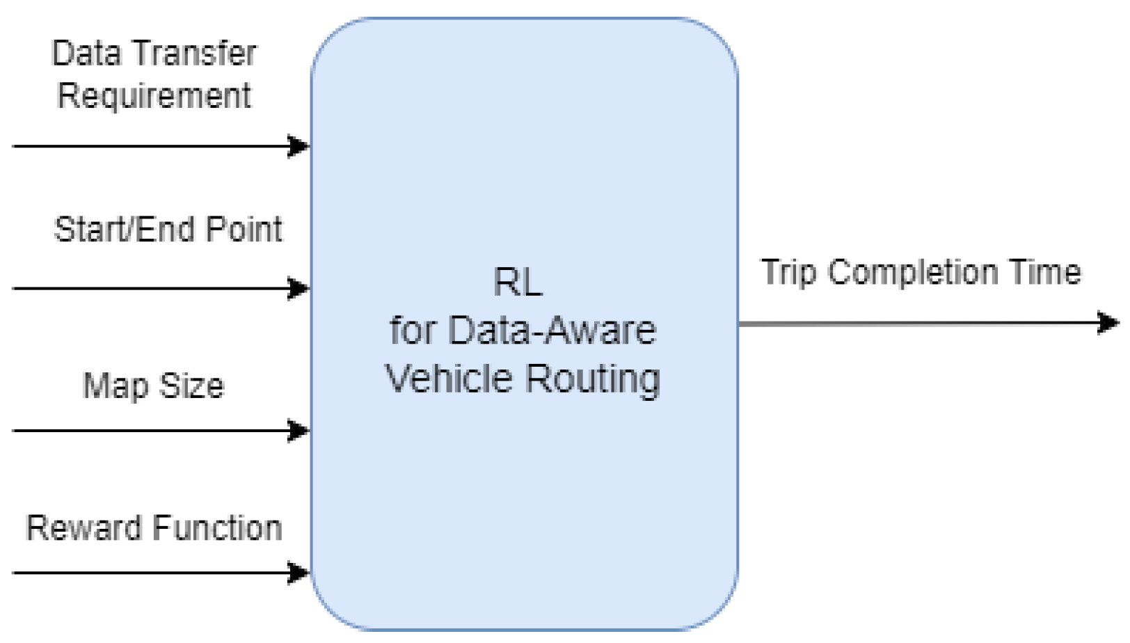
3.3. Experiment Setup

In the setup of our experiment, we adopted a structured approach to define the environment for our agent’s operation, along with predetermined constants that framed the experimental conditions. An important stipulation in our experimental design is that the agent is required to transfer a specified quantity of data before reaching its destination. Data transfer by the agent, denoted by D (in bits), is influenced by the bandwidth B available on a road link (in bits per second) and the duration T the agent spends on that link (in seconds). For a given road link i, the potential data transfer $D_i$ can initially be approximated as follows:

$$D_i=B_i·T_i$$

(1)

Equation (1) assumes optimal conditions in which the agent uses the maximum bandwidth rate of the road. However, this model requires refinement due to the presence of other agents in the network, which share the road and its available bandwidth. Thus, a more realistic approach to model the data transfer on road i incorporates the traffic density or congestion $\gamma$, modifying the equation to

$$D_i=\left({\displaystyle \frac{B_i}{\alpha ·{\gamma }_i}}\right)·T_i$$

(2)

This adjustment scales the data transfer rate of each link inversely with congestion, reflecting the reduced bandwidth available to an agent as traffic density increases. To guarantee that congestion can only decrease effective bandwidth, we require $\alpha {\gamma }_i\ge 1$ for every road link and choose $\alpha =1+{\sigma }_{\gamma }$, where ${\sigma }_{\gamma }$ is the standard deviation of the congestion values across the map. For our dataset, this gives $\alpha \approx 1.5$, which keeps the denominator safely above one and normalizes congestion impact network-wide. Sweeping $\alpha$ over $[1.2,2.0]$ altered the mean trip completion time by less than 3%, indicating that the learned policy is robust to reasonable choices of $\alpha$. Thus, the adjustment both normalizes traffic effects and ensures that the effective bandwidth $B_i/$ doesn’t increase, fully consistent with the model’s design premise.

To quantify road congestion, we used our preprocessed data, including the average speed and time spent traveling between nodes, along with the distances between these nodes, to find a normalized congestion factor for each road link i. This factor inversely impacts the bandwidth available to each agent, with higher traffic densities leading to a reduced bandwidth per user.

Bandwidth availability across the road network is modeled by introducing strategically positioned base stations in the city. These base stations create zones of varying bandwidth intensity, with roads within the inner radius of a station receiving maximum bandwidth. The bandwidth allocation decreases for each subsequent radius away from a station until the outer radius is reached. In cases where a road falls within the coverage area of multiple base stations, the bandwidth is determined by the strongest signal or highest value from among the relevant stations, thus optimizing data transfer capabilities in areas with dense coverage. An illustration of this can be seen in Figure 4.

With the bandwidth and traffic parameters carefully defined and quantified, our experimental framework was equipped to assess the amount of data that an agent could feasibly transfer while traversing each road link within the urban network. We noted that the same MDP structure can be extended to additional objectives, such as electric vehicle battery management, by appending an energy state variable and corresponding actions; details are discussed in the Future Work Section.

This comprehensive setup provides a robust foundation for testing and validating our reinforcement learning-based approach to autonomous vehicle path planning and data transfer in complex urban environments. Moreover, the methodology is highly generalizable and can be applied to other maps and datasets, provided that the relevant type of data is available.

3.4. Simulation Setup

We employed tabular Q-learning [46] rather than a deep function approximator because, after a lossless discretization, the state space remained small enough for an exact table. Node location is inherently discrete ($\left|X\right|=4327$ nodes), the remaining data d are bucketed into 20 equal-width bins (0–5 MB, …, 95–100 MB), and both bandwidth and traffic density on outgoing links are mapped to four quartile-based levels. At the start of every episode, all link speeds and bandwidths are resampled from their empirical distributions, so the agent faces a different traffic and wireless landscape each run.

This yields:

$$\left|S\right|=4327\times 20\times 4\times 4=1.38\times {10}^6$$

Distinct state tuples—an $\sim 8\mathrm{MB}$ Q-table when stored sparsely via a collision-resistant hash map—are well within commodity GPU memory.

Given this tractable size, tabular Q-learning offers exact value estimates with guaranteed convergence in finite MDPs, thus maximizing reproducibility and algorithmic transparency. Unvisited state–action pairs are initialized optimistically, and an $\epsilon$-greedy schedule decays linearly from $0.9$ to $0.05$ over the first 200,000 interaction steps, speeding up convergence without resorting to deep neural networks.

Q-values are updated with the learning rate $\alpha =0.10$ and discount factor $\gamma =0.99$. Each episode terminates upon arrival at the destination or after 4000 simulation steps. $\epsilon$ in the $\epsilon$-greedy policy decays linearly from 0.90 to 0.05 over the first $2\times {10}^5$ steps. Optimistic initial Q-values were set to $+50$ s to encourage exploration.

Figure 5 depicts the key parameters that influence the performance of our agent, measured by trip completion time. These include the data transfer requirement, which specifies the volume of data to be transferred prior to the agent reaching its destination; the start and end points, which set the trip’s length; the map size, which reflects the extent of the state space; and the reward function, which shapes the agent’s behavior in this environment. To explore the impact of a specific parameter, we vary one parameter at a time, keeping the others constant.

4. Experiments and Results

In this section, we present the experiments conducted to evaluate the effectiveness of our proposed reinforcement learning-based approach to path planning for autonomous vehicles in urban environments. These experiments are crucial in demonstrating how our model addresses the dual challenges of optimizing driving time and ensuring timely data transfer. We aim to highlight the distinct advantages of our approach over conventional path planning methods that do not account for the complex interplay between traffic and bandwidth heterogeneity. To accomplish this, we conducted three experiments based on the simulation parameters illustrated in Figure 5. First, we assessed our reinforcement learning agent’s performance against general baselines with varying reward functions. For this experiment, we investigated the performance of our agent with different start and end points to determine how effectively our approach manages trips of varying lengths. Next, we compared the performance of our trained agent when the data transfer requirement parameter is varied. Finally, we examined the impact of different map sizes on our agent’s performance to evaluate the scalability of our solution.

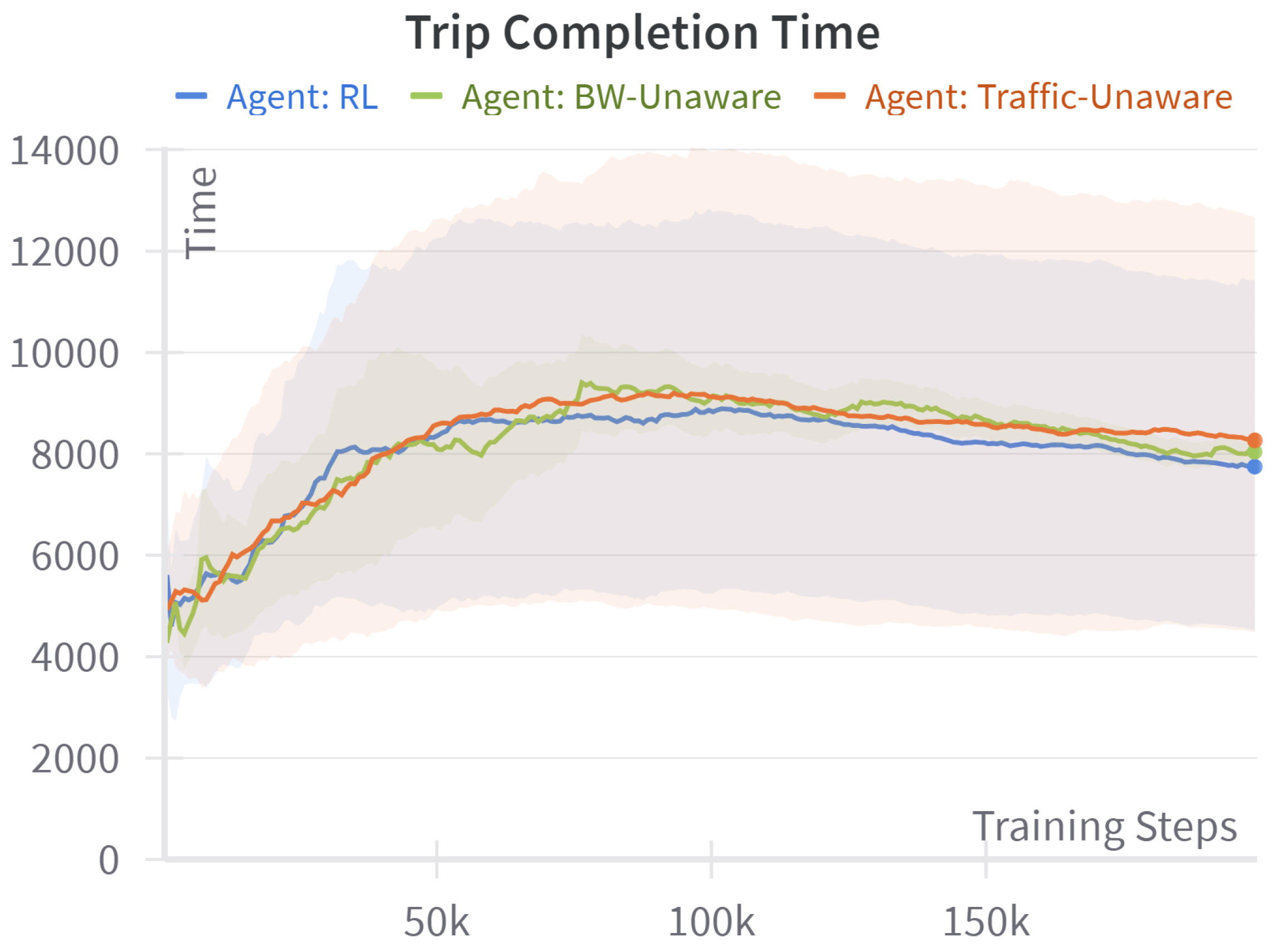
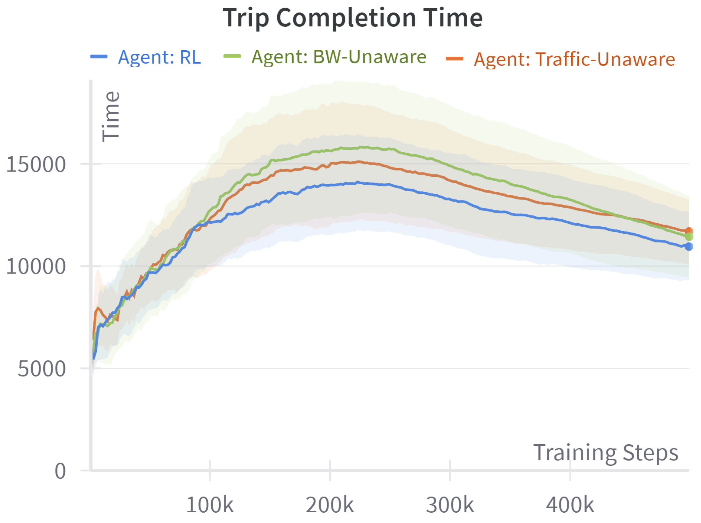
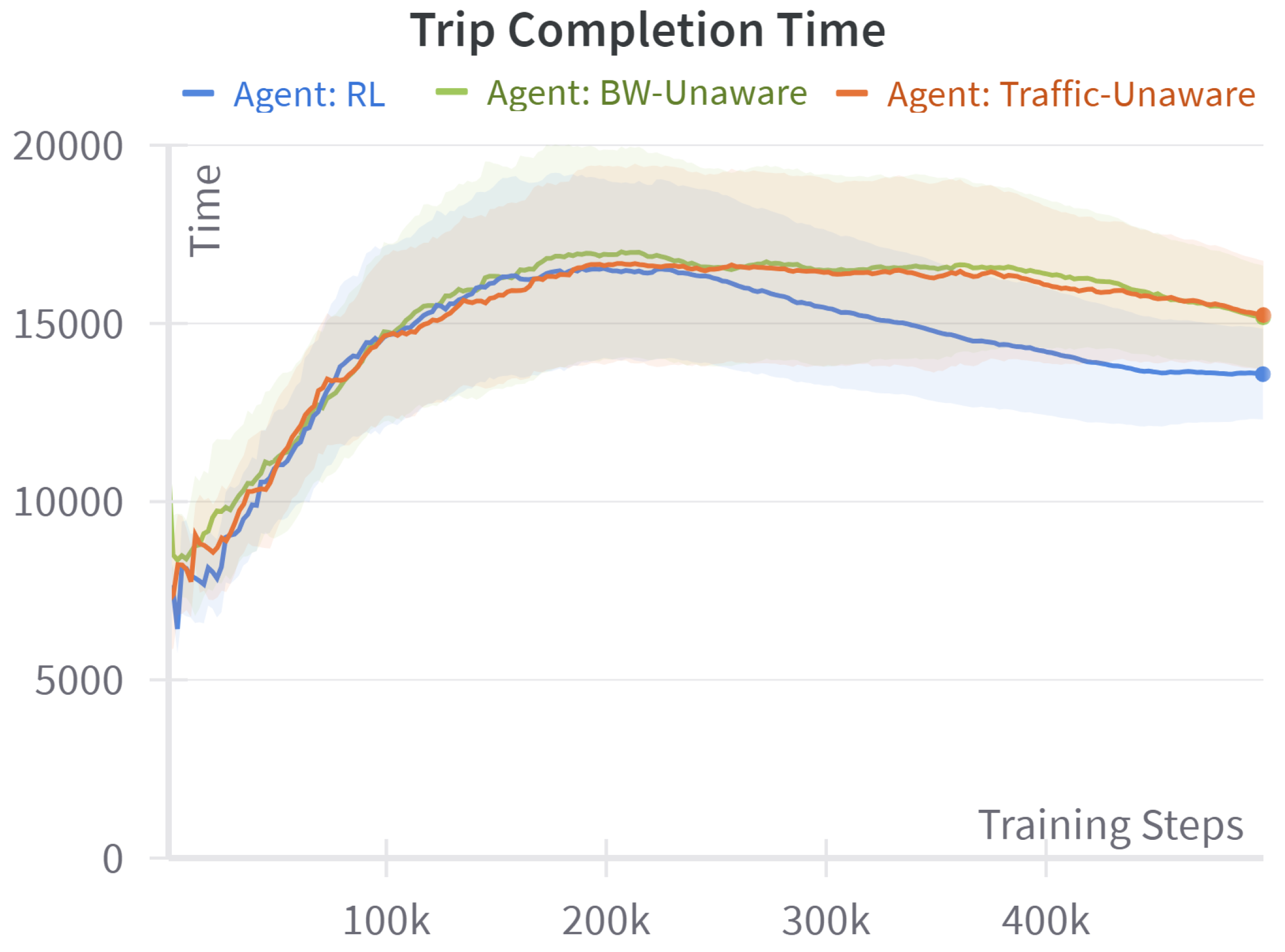
4.1. Baseline Comparison

For our first set of experiments, we compared the proposed RL agent with two classical planning baselines that are already implicit in our environment:

• Traffic-unaware (shortest path): When the traffic-delay term is removed from the reward, every edge has a unit cost; the resulting policy is exactly the static shortest hop route returned by Dijkstra’s algorithm, a standard distance-optimal algorithm.
• Bandwidth-unaware (fastest path): When the data-throughput term is omitted, the reward reduces to negative travel time. The baseline therefore behaves like a time-dependent fastest path algorithm that minimizes congestion-aware travel time while ignoring any data-transfer objective.

Only the reward weights are altered to create these baselines; all other parameters in Figure 5 remain unchanged. To demonstrate robustness across different journeys, we evaluated each agent on short, medium, and long trips.

Figure 6 shows the learning curves for a representative short-trip scenario. The RL agent converges slightly faster than both classical baselines and attains the lowest mean trip completion time. The performance gap is modest, as expected for short routes with few alternatives, but still demonstrates a consistent advantage over the shortest path and fastest path baselines.

Figure 6 compares the performance of our trained agent to the baseline agents during a short trip. We observed that our trained agent learns the fastest because it converges slightly faster than the baselines and that our agent also converges at a lower trip completion time, slightly outperforming the compared baselines. In this experiment, the small differences in performance between our trained agent and the baselines are primarily due to the short duration of the trip and the limited variety of available route options the agent can take.

We repeated the evaluation for a medium-length trip, as shown in Figure 7. Here, the advantage of the RL agent becomes more pronounced: it reaches its asymptotic performance faster than both classical baselines and settles at a lower mean completion time. This gap widens because longer journeys expose more opportunities for the RL policy to trade off bandwidth and congestion, whereas the classical baselines optimize only a single criterion.

Finally, in the long-trip scenario shown in Figure 8, the RL agent widens its advantage even further. It converges noticeably sooner than the fastest path baseline and completes the journey in appreciably less time than the shortest path baseline. These observations confirm that as trip length increases, the proposed multi-objective policy continues to outperform the classical single-objective methods—both in learning speed and in steady-state efficiency.

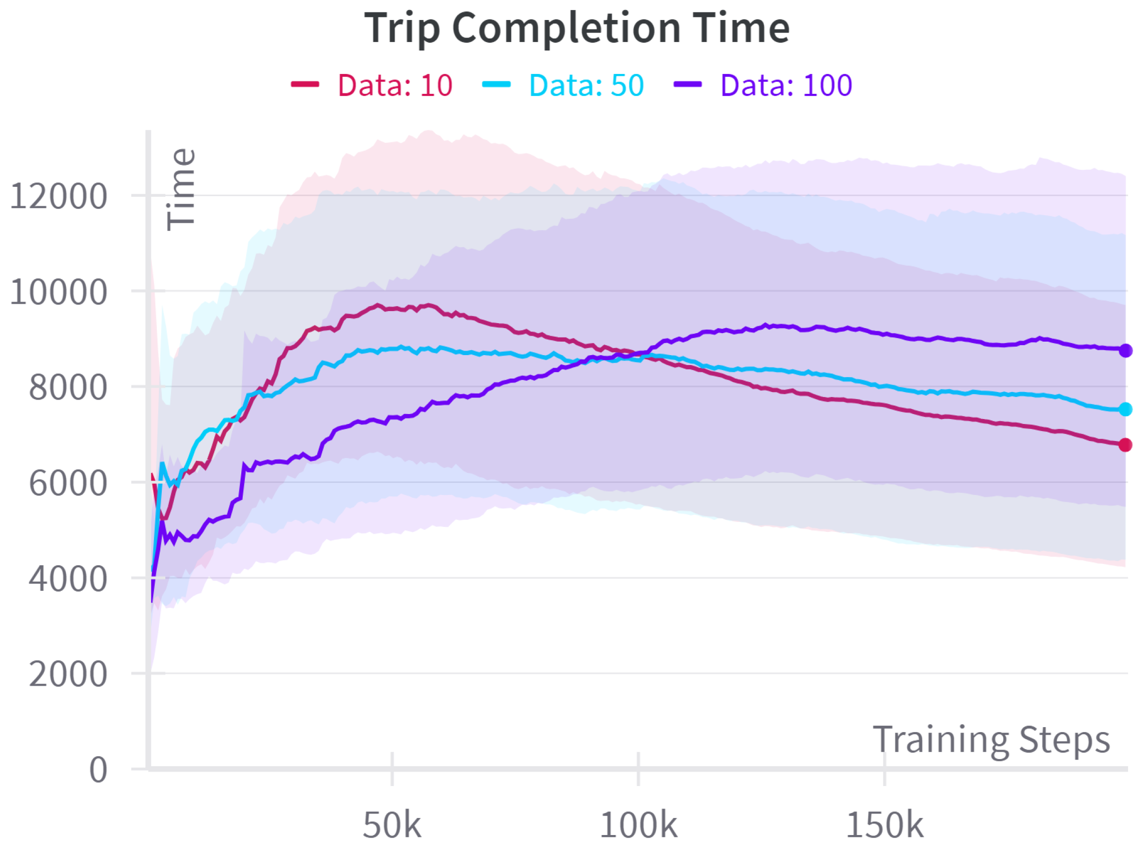
4.2. Data Requirement Comparison

In this experiment, we compared the performance of our trained agent when the data transfer requirement parameter is varied. This parameter denotes the amount of data that needs to be transferred before an agent reaches its destination.

We choose to run this experiment on a short trip length for several compelling reasons. The short trip offers a more controlled environment with fewer confounding variables, allowing us to isolate and measure the direct impact of the data requirement parameter more accurately. Furthermore, these conditions simplify the decision-making process for the reinforcement learning agent and allow for faster iterations of tests, thus providing a clearer analysis of how data requirements influence route selection.

We can observe from Figure 9 that a lower data transfer requirement leads to a faster trip overall. This outcome aligns with our expectations, as the quicker the agent completes its data transfer, the sooner it can focus on completing the trip as fast as possible.

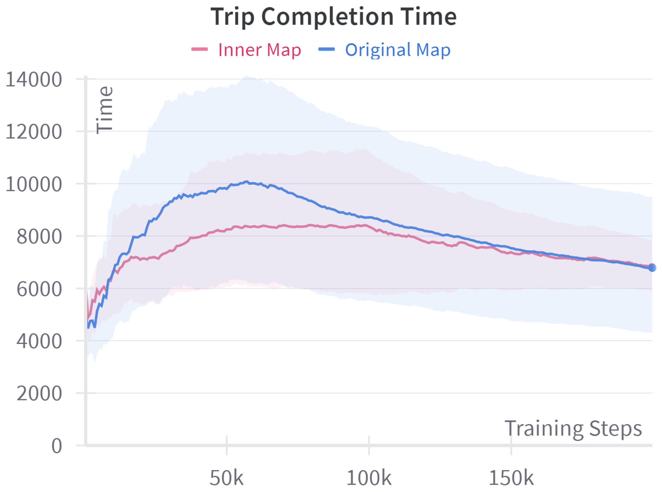
4.3. Map Size Comparison

In this experiment, we investigated how different map sizes affect the performance of our trained agent. The map size parameter defines the state space of our environment, which allows us to evaluate the scalability of our solution. We kept our focus on short trip lengths, consistent with the approach used in our previous experiment. The rationale for this choice remains the same as previously discussed, leveraging the benefits of a more controlled environment and simplified decision-making process for our reinforcement learning agent.

We analyzed two distinct maps, namely the original map and a smaller inner map. The original map, as shown in Figure 3, was used consistently throughout our experiments. The inner map is a centrally positioned, cropped version of the original, with half the length and width of the original map. As a result, it covers only one-fourth of the total area of the original map. Despite being cropped, it retains the same level of detail as the original, focusing on a specific central area.

Figure 10 demonstrates that our trained agent achieves similar completion times on both the inner and original maps, with the inner map showing faster convergence. This difference in convergence speed is due to the inner map’s smaller area, which enables more efficient exploration and strategy optimization. The original map initially exhibits greater performance variability, as shown by its wider confidence interval, which narrows as training progresses. Our approach’s key strength lies in its scalability, as it effectively adapts to different environment sizes without significant performance loss. This experiment emphasizes the advantage of using a reduced state space for quicker training and convergence while also highlighting the successful application of learned strategies to larger, more complex environments. These findings emphasize the robustness and scalability of our solution across diverse scenarios.

5. Conclusions

We have addressed the challenges of path planning for autonomous vehicles within urban environments, prioritizing both timely data transfer and efficient travel. Our novel reinforcement learning solution effectively navigates these complex challenges, demonstrating significant advantages over baseline methods. To evaluate this approach, we implemented a GraphML-based simulation environment that integrates real-world map data and vehicle mobility patterns. This environment accurately represented the dynamic and complex nature of urban traffic, providing a robust platform to test our reinforcement learning strategies.

Our findings demonstrate that our reinforcement learning approach is not only viable but also advantageous for path planning in environments characterized by heterogeneous traffic and high data transfer demands. We have shown that our proposed solution is scalable and consistently outperforms standard baseline models across different trip lengths.

Despite these encouraging results, several limitations should be acknowledged. First, all performance curves were generated from a single random seed; although this seed is representative, reinforcement learning outcomes can vary significantly with initialization. To address this, future work will average results over multiple seeds, reporting mean performance metrics with corresponding 95% confidence intervals to ensure full statistical robustness.

Another limitation is the static nature of traffic and bandwidth conditions within individual simulation episodes and the evaluation involving only a single vehicle. To enhance realism and adaptability, future studies will incorporate online perturbations, such as sudden congestion spikes, temporary bandwidth blackouts, and forced rerouting scenarios. Additionally, expanding the simulation environment to include multiple autonomous vehicles interacting on the same road network and sharing wireless spectra will allow for an investigation into cooperative routing and resource allocation strategies.

To further improve our model, replacing the current tabular critic with a graph-aware deep Q-network or an actor–critic architecture is a logical next step. This modification would facilitate end-to-end learning directly from continuous traffic and bandwidth features while preserving the scalability demonstrated in this work. Furthermore, broadening the baseline comparisons by benchmarking against advanced deterministic algorithms such as time-dependent A* and multi-objective label-setting algorithms would provide richer context for evaluating our reinforcement learning approach.

Additionally, transitioning from a fixed-weight scalarization approach to explicit multi-objective reinforcement learning techniques, such as Pareto-front approximation or constrained-policy optimization, would allow fleet operators to visualize and select from the complete trade-off curve between travel time and data throughput rather than relying on a single pre-tuned weight vector.

Finally, an exciting extension of our framework involves incorporating electric vehicle (EV) energy management. By augmenting the state space with a battery-level variable and integrating "visit-charging-station" actions at nodes equipped with charging stations, future agents could learn policies that optimize travel time, data transfer, and energy replenishment simultaneously. This enhancement would highlight the generalizability of our reinforcement learning framework to broader smart mobility challenges and align closely with contemporary EV routing research trends. Given the additive nature of our reward function, incorporating battery management penalties and charging station costs would require only minor modifications, enabling seamless integration into the existing framework.

The versatility and adaptability of our simulation environment thus extend beyond the scope of our initial evaluations, offering extensive potential for further research into varying vehicle autonomy levels, emerging communication technologies, multi-agent scenarios, and the integration of real-time data from smart city infrastructure. Such explorations are vital for addressing evolving urban mobility challenges and the increasing data demands of connected vehicles.

References

1. Intel Corporation. Data Is the New Oil in the Future of Automated Driving. 2016. Available online: https://www.intel.com/content/www/us/en/newsroom/news/self-driving-cars-data.html (accessed on 10 March 2024).
2. You, C.; Lu, J.; Filev, D.; Tsiotras, P. Advanced planning for autonomous vehicles using reinforcement learning and deep inverse reinforcement learning. Robot. Auton. Syst. 2019, 114, 1–18. [Google Scholar] [CrossRef]
3. Singh, S. Critical Reasons for Crashes Investigated in the National Motor Vehicle Crash Causation Survey; Technical Report; National Highway Traffic Safety Administration: Washington, DC, USA, 2015. Available online: https://crashstats.nhtsa.dot.gov/Api/Public/ViewPublication/812506 (accessed on 10 March 2024).
4. Ibáñez, J.A.G.; Zeadally, S.; Contreras-Castillo, J. Integration challenges of intelligent transportation systems with connected vehicle, cloud computing, and internet of things technologies. IEEE Wirel. Commun. 2015, 22, 122–128. [Google Scholar] [CrossRef]
5. Taha, A.E.M.; Abuali, N.A. Route planning considerations for autonomous vehicles. IEEE Commun. Mag. 2018, 56, 78–84. [Google Scholar] [CrossRef]
6. Ye, H.; Liang, L.; Li, G.Y.; Kim, J.; Lu, L.; Wu, M. Machine learning for vehicular networks: Recent advances and application examples. IEEE Veh. Technol. Mag. 2017, 13, 94–101. [Google Scholar] [CrossRef]
7. Brandes, U.; Eiglsperger, M.; Lerner, J.; Pich, C. Graph markup language (GraphML). In Handbook of Graph Drawing and Visualization; Chapman and Hall/CRC: Boca Raton, FL, USA, 2013. [Google Scholar] [CrossRef]
8. Ming, Y.; Li, Y.; Zhang, Z.; Yan, W. A survey of path planning algorithms for autonomous vehicles. SAE Int. J. Commer. Veh. 2021, 14, 97–109. [Google Scholar] [CrossRef]
9. Marin-Plaza, P.; Hussein, A.; Martin, D.; de la Escalera, A. Global and local path planning study in a ROS-based research platform for autonomous vehicles. J. Adv. Transp. 2018, 2018, 6392697. [Google Scholar] [CrossRef]
10. Dijkstra, E.W. A note on two problems in connection with graphs. Numer. Math. 1959, 1, 269–271. [Google Scholar] [CrossRef]
11. Hart, P.E.; Nilsson, N.J.; Raphael, B. A formal basis for the heuristic determination of minimum cost paths. IEEE Trans. Syst. Sci. Cybern. 1968, 4, 100–107. [Google Scholar] [CrossRef]
12. Dechter, R.; Pearl, J. Generalized best-first search strategies and the optimality of A*. J. ACM 1985, 32, 505–536. [Google Scholar] [CrossRef]
13. Paden, B.; Čáp, M.; Yong, S.Z.; Yershov, D.; Frazzoli, E. A survey of motion planning and control techniques for self-driving urban vehicles. IEEE Trans. Intell. Veh. 2016, 1, 33–55. [Google Scholar] [CrossRef]
14. Bast, H.; Delling, D.; Goldberg, A.V.; Müller-Hannemann, M.; Pajor, T.; Sanders, P.; Wagner, D.; Werneck, R.F. Route planning in transportation networks. In Algorithm Engineering; Springer: Berlin/Heidelberg, Germany, 2016. [Google Scholar] [CrossRef]
15. Stentz, A. Optimal and efficient path planning for partially-known environments. In Proceedings of the 1994 IEEE International Conference on Robotics and Automation, San Diego, CA, USA, 8–13 May 1994; pp. 3310–3317. [Google Scholar] [CrossRef]
16. Nguyen, H.H.; Kim, D.H.; Kim, C.K.; Yim, H.; Jeong, S.K.; Kim, S.B. A simple path planning for automatic guided vehicle in unknown environment. In Proceedings of the 2017 14th International Conference on Ubiquitous Robots and Ambient Intelligence (URAI), Jeju, Republic of Korea, 28 June–1 July 2017; pp. 337–341. [Google Scholar] [CrossRef]
17. Khatib, O. Real-time obstacle avoidance for manipulators and mobile robots. In Autonomous Robot Vehicles; Springer: Berlin/Heidelberg, Germany, 1990; pp. 396–404. [Google Scholar] [CrossRef]
18. Ganeshmurthy, M.S.; Suresh, G.R. Path planning algorithm for autonomous mobile robot in dynamic environment. In Proceedings of the 2015 3rd International Conference on Signal Processing, Communication and Networking, Chennai, India, 26–28 March 2015. [Google Scholar] [CrossRef]
19. Wang, L.; Luo, C. A hybrid genetic tabu search algorithm for mobile robot to solve AS/RS path planning. Int. J. Robot. Autom. 2018, 33. [Google Scholar] [CrossRef]
20. LaValle, S. Rapidly-exploring random trees: A new tool for path planning. Annu. Res. Rep. 1998. [Google Scholar]
21. Kiran, B.R.; Sobh, I.; Talpaert, V.; Mannion, P.; Sallab, A.A.A.; Yogamani, S.; Pérez, P. Deep reinforcement learning for autonomous driving: A survey. IEEE Trans. Intell. Transp. Syst. 2020, 23, 4909–4926. [Google Scholar] [CrossRef]
22. Nešmark, J.I.; Fufaev, N.A. Dynamics of Nonholonomic Systems; American Mathematical Society: Providence, RI, USA, 2004. [Google Scholar] [CrossRef]
23. LaValle, S.M.; Kuffner, J.J. Randomized kinodynamic planning. In Proceedings of the 1999 IEEE International Conference on Robotics and Automation (Cat. No.99CH36288C), Detroit, MI, USA, 10–15 May 1999; Volume 1, pp. 473–479. [Google Scholar] [CrossRef]
24. Loaiza Quintana, C.; Climent, L.; Arbelaez, A. Iterated Local Search for the eBuses Charging Location Problem. In Proceedings of the Parallel Problem Solving from Nature—PPSN XVII: 17th International Conference, Dortmund, Germany, 10–14 September 2022; Springer: Berlin/Heidelberg, Germany, 2022. [Google Scholar] [CrossRef]
25. Nasrabadi, N.M. Pattern recognition and machine learning. J. Electron. Imaging 2007, 16, 049901. [Google Scholar] [CrossRef]
26. Yu, D.; Deng, L. Deep learning and its applications to signal and information processing. IEEE Signal Process. Mag. 2011, 28, 145–154. [Google Scholar] [CrossRef]
27. Hinton, G.; Deng, L.; Yu, D.; Dahl, G.E.; Mohamed, A.; Jaitly, N.; Senior, A.; Vanhoucke, V.; Nguyen, P.; Sainath, T.N.; et al. Deep neural networks for acoustic modeling in speech recognition: The shared views of four research groups. IEEE Signal Process. Mag. 2012, 29, 82–97. [Google Scholar] [CrossRef]
28. Graves, A.; Mohamed, A.; Hinton, G. Speech recognition with deep recurrent neural networks. arXiv 2013, arXiv:1303.5778. [Google Scholar] [CrossRef]
29. Kumar, A.; Irsoy, O.; Ondruska, P.; Iyyer, M.; Bradbury, J.; Gulrajani, I.; Zhong, V.; Paulus, R.; Socher, R. Ask me anything: Dynamic memory networks for natural language processing. arXiv 2015, arXiv:1506.07285. [Google Scholar] [CrossRef]
30. Otter, D.W.; Medina, J.R.; Kalita, J.K. A survey of the usages of deep learning for natural language processing. IEEE Trans. Neural Netw. Learn. Syst. 2020, 32, 604–624. [Google Scholar] [CrossRef]
31. Manning, C.; Surdeanu, M.; Bauer, J.; Finkel, J.; Bethard, S.; McClosky, D. The Stanford CoreNLP natural language processing toolkit. In Proceedings of the 52nd Annual Meeting of the Association for Computational Linguistics: System Demonstrations, Baltimore, MD, USA, 23–24 June 2014; pp. 55–60. [Google Scholar] [CrossRef]
32. Collobert, R.; Weston, J. A unified architecture for natural language processing: Deep neural networks with multitask learning. In Proceedings of the 25th International Conference on Machine Learning, Helsinki, Finland, 5–9 July 2008; pp. 160–167. [Google Scholar] [CrossRef]
33. Kononenko, I. Machine learning for medical diagnosis: History, state of the art and perspective. Artif. Intell. Med. 2001, 23, 89–109. [Google Scholar] [CrossRef]
34. Shvets, A.A.; Rakhlin, A.; Kalinin, A.A.; Iglovikov, V.I. Automatic instrument segmentation in robot-assisted surgery using deep learning. In Proceedings of the 17th IEEE International Conference on Machine Learning and Applications, Orlando, FL, USA, 17–20 December 2018; pp. 624–628. [Google Scholar] [CrossRef]
35. Sutton, R.S.; Barto, A.G. Reinforcement learning: An introduction. IEEE Trans. Neural Netw. 1988, 9, 1054. [Google Scholar] [CrossRef]
36. Bae, H.; Kim, G.D.; Kim, J.; Qian, D.; Lee, S.G. Multi-robot path planning method using reinforcement learning. Appl. Sci. 2019, 9, 3057. [Google Scholar] [CrossRef]
37. Ge, S.S.; Cui, Y.J. New potential functions for mobile robot path planning. IEEE Trans. Robot. Autom. 2000, 16, 615–620. [Google Scholar] [CrossRef]
38. Zhang, Y.; Gong, D.; Zhang, J. Robot path planning in uncertain environment using multi-objective particle swarm optimization. Neurocomputing 2013, 103, 172–185. [Google Scholar] [CrossRef]
39. Tharwat, A.; Elhoseny, M.; Hassanien, A.E.; Gabel, T.; Kumar, A. Intelligent Bézier curve-based path planning model using chaotic particle swarm optimization algorithm. Clust. Comput. 2019, 22, 4745–4766. [Google Scholar] [CrossRef]
40. Elhoseny, M.; Tharwat, A.; Hassanien, A.E. Bezier curve based path planning in a dynamic field using modified genetic algorithm. J. Comput. Sci. 2018, 25, 339–350. [Google Scholar] [CrossRef]
41. Alomari, A.; Comeau, F.; Phillips, W.; Aslam, N. New path planning model for mobile anchor-assisted localization in wireless sensor networks. Wirel. Netw. 2018, 24, 2589–2607. [Google Scholar] [CrossRef]
42. Peters, J.; Schaal, S. Natural actor-critic. Neurocomputing 2008, 71, 1180–1190. [Google Scholar] [CrossRef]
43. Bhasin, S.; Kamalapurkar, R.; Johnson, M.; Vamvoudakis, K.G.; Lewis, F.L.; Dixon, W.E. A novel actor–critic–identifier architecture for approximate optimal control of uncertain nonlinear systems. Automatica 2013, 49, 82–92. [Google Scholar] [CrossRef]
44. Vamvoudakis, K.G.; Lewis, F.L. Online actor–critic algorithm to solve the continuous-time infinite horizon optimal control problem. Automatica 2010, 46, 878–888. [Google Scholar] [CrossRef]
45. Florensa, C.; Degrave, J.; Heess, N.; Springenberg, J.T.; Riedmiller, M. Self-supervised learning of image embedding for continuous control. arXiv 2019, arXiv:1901.00943. [Google Scholar] [CrossRef]
46. Watkins, C.J.C.H.; Dayan, P. Q-learning. Mach. Learn. 1992, 8, 279–292. [Google Scholar] [CrossRef]
47. Lillicrap, T.P.; Hunt, J.J.; Pritzel, A.; Heess, N.; Erez, T.; Tassa, Y.; Silver, D.; Wierstra, D. Continuous control with deep reinforcement learning. arXiv 2015, arXiv:1509.02971. [Google Scholar] [CrossRef]
48. Kofinas, P.; Dounis, A.I.; Vouros, G.A. Fuzzy Q-learning for multi-agent decentralized energy management in microgrids. Appl. Energy 2018, 219, 53–67. [Google Scholar] [CrossRef]
49. Dowling, J.; Curran, E.; Cunningham, R.; Cahill, V. Using feedback in collaborative reinforcement learning to adaptively optimize MANET routing. IEEE Trans. Syst. Man Cybern.—Part A Syst. Hum. 2005, 35, 360–372. [Google Scholar] [CrossRef]
50. Doddalinganavar, S.S.; Tergundi, P.V.; Patil, R.S. Survey on deep reinforcement learning protocol in VANET. In Proceedings of the 1st International Conference on Advances in Information Technology, Chikmagalur, India, 25–27 July 2019; pp. 81–86. [Google Scholar] [CrossRef]
51. Liu, J.; Wang, Q.; He, C.; Jaffrès-Runser, K.; Xu, Y.; Li, Z.; Xu, Y. QMR: Q-learning based multi-objective optimization routing protocol for flying ad hoc networks. Comput. Commun. 2020, 150, 304–316. [Google Scholar] [CrossRef]
52. Coutinho, W.P.; Battarra, M.; Fliege, J. The unmanned aerial vehicle routing and trajectory optimisation problem, a taxonomic review. Comput. Ind. Eng. 2018, 120, 116–128. [Google Scholar] [CrossRef]
53. Nazib, R.A.; Moh, S. Reinforcement learning-based routing protocols for vehicular ad hoc networks: A comparative survey. IEEE Access 2021, 9, 27552–27587. [Google Scholar] [CrossRef]
54. Li, F.; Song, X.; Chen, H.; Li, X.; Wang, W. Hierarchical routing for vehicular ad hoc networks via reinforcement learning. IEEE Trans. Veh. Technol. 2019, 68, 1852–1865. [Google Scholar] [CrossRef]
55. Misra, S.; Woungang, I.; Misra, S.C. Guide to Wireless Ad Hoc Networks; Springer Science & Business Media: Berlin/Heidelberg, Germany, 2009. [Google Scholar] [CrossRef]
56. Hartenstein, H.; Laberteaux, K. VANET: Vehicular Applications and Inter-Networking Technologies; John Wiley & Sons: Hoboken, NJ, USA, 2009. [Google Scholar] [CrossRef]
57. Vigo, D.; Toth, P. (Eds.) Vehicle Routing; MOS-SIAM Series on Optimization; Society for Industrial and Applied Mathematics: Philadelphia, PA, USA, 2014. [Google Scholar] [CrossRef]
58. Rasheed, A.; Gillani, S.; Ajmal, S.; Qayyum, A. Vehicular ad hoc network (VANET): A survey, challenges, and applications. In Proceedings of the Vehicular Ad-Hoc Networks for Smart Cities; Advances in Intelligent Systems and Computing. Springer: Berlin/Heidelberg, Germany, 2017; pp. 39–51. [Google Scholar] [CrossRef]
59. Li, F.; Wang, Y. Routing in vehicular ad hoc networks: A survey. IEEE Veh. Technol. Mag. 2007, 2, 12–22. [Google Scholar] [CrossRef]
60. Kaelbling, L.P.; Littman, M.L.; Moore, A.W. Reinforcement learning: A survey. J. Artif. Intell. Res. 1996, 4, 237–285. [Google Scholar] [CrossRef]
61. Chettibi, S.; Chikhi, S. A survey of reinforcement learning based routing protocols for mobile ad-hoc networks. In Proceedings of the Recent Trends in Wireless and Mobile Networks, Ankara, Turkey, 26–28 June 2011; Communications in Computer and Information Science. Springer: Berlin/Heidelberg, Germany, 2011; pp. 1–13. [Google Scholar] [CrossRef]
62. McCall, J.C.; Trivedi, M.M. Video-based lane estimation and tracking for driver assistance: Survey, system, and evaluation. IEEE Trans. Intell. Transp. Syst. 2006, 7, 20–37. [Google Scholar] [CrossRef]
63. Keen, S.D.; Cole, D.J. Application of time-variant predictive control to modelling driver steering skill. Veh. Syst. Dyn. 2011, 49, 527–559. [Google Scholar] [CrossRef]
64. You, C.; Tsiotras, P. Optimal two-point visual driver model and controller development for driver-assist systems for semi-autonomous vehicles. In Proceedings of the 2016 American Control Conference (ACC), Boston, MA, USA, 6–8 July 2016; pp. 5976–5981. [Google Scholar] [CrossRef]
65. Zafeiropoulos, S.; Tsiotras, P. Design of a lane-tracking driver steering assist system and its interaction with a two-point visual driver model. In Proceedings of the 2014 American Control Conference, Portland, OR, USA, 4–6 June 2014; pp. 3911–3917. [Google Scholar] [CrossRef]
66. Lange, S.; Riedmiller, M.; Voigtländer, A. Autonomous reinforcement learning on raw visual input data in a real world application. In Proceedings of the 2012 International Joint Conference on Neural Networks (IJCNN), Brisbane, QLD, Australia, 10–15 June 2012; pp. 1–8. [Google Scholar] [CrossRef]
67. Zhu, M.; Wang, X.; Wang, Y. Human-like autonomous car-following model with deep reinforcement learning. Transp. Res. Part C Emerg. Technol. 2018, 97, 348–368. [Google Scholar] [CrossRef]
68. Sallab, A.; Abdou, M.; Perot, E.; Yogamani, S. End-to-End Deep Reinforcement Learning for Lane Keeping Assist. arXiv 2016, arXiv:1612.04340. [Google Scholar] [CrossRef]
69. Min, K.; Kim, H.; Huh, K. Deep distributional reinforcement learning based high-level driving policy determination. IEEE Trans. Intell. Veh. 2019, 4, 416–424. [Google Scholar] [CrossRef]
70. Bouton, M.; Nakhaei, A.; Fujimura, K.; Kochenderfer, M.J. Cooperation-aware reinforcement learning for merging in dense traffic. In Proceedings of the IEEE Intelligent Transportation Systems Conference, Auckland, New Zealand, 27–30 October 2019; pp. 3441–3447. [Google Scholar] [CrossRef]
71. Chen, D.; Hajidavalloo, M.R.; Li, Z.; Chen, K.; Wang, Y.; Jiang, L.; Wang, Y. Deep multi-agent reinforcement learning for highway on-ramp merging in mixed traffic. IEEE Trans. Intell. Transp. Syst. 2023, 24, 11623–11638. [Google Scholar] [CrossRef]
72. Fu, Y.; Li, C.; Yu, F.R.; Luan, T.H.; Zhang, Y. A decision-making strategy for vehicle autonomous braking in emergency via deep reinforcement learning. IEEE Trans. Veh. Technol. 2020, 69, 5876–5888. [Google Scholar] [CrossRef]
73. Xie, J.; Xu, X.; Wang, F.; Liu, Z.; Chen, L. Coordination control strategy for human-machine cooperative steering of intelligent vehicles: A reinforcement learning approach. IEEE Trans. Intell. Transp. Syst. 2022, 23, 21163–21177. [Google Scholar] [CrossRef]
74. Haydari, A.; Yılmaz, Y. Deep reinforcement learning for intelligent transportation systems: A survey. IEEE Trans. Intell. Transp. Syst. 2020, 23, 11–32. [Google Scholar] [CrossRef]
75. Fei, Y.; Xing, L.; Yao, L.; Yang, Z.; Zhang, Y. Deep reinforcement learning for decision making of autonomous vehicles in non-lane-based traffic environments. PLoS ONE 2025, 20, e0320578. [Google Scholar] [CrossRef] [PubMed]
76. Hussain, Q.; Noor, A.; Qureshi, M.; Li, J.; Rahman, A.; Bakry, A.; Mahmood, T.; Rehman, A. Reinforcement learning based route optimization model to enhance energy efficiency in internet of vehicles. Sci. Rep. 2025, 15, 3113. [Google Scholar] [CrossRef] [PubMed]
77. Sun, P.; He, J.; Wan, J.; Guan, Y.; Liu, D.; Su, X.; Li, L. Deep reinforcement learning based low energy consumption scheduling approach design for urban electric logistics vehicle networks. Sci. Rep. 2025, 15, 9003. [Google Scholar] [CrossRef] [PubMed]
78. Wang, X.; Qian, B.; Zhuo, J.; Liu, W. An Autonomous Vehicle Behavior Decision Method Based on Deep Reinforcement Learning with Hybrid State Space and Driving Risk. Sensors 2025, 25, 774. [Google Scholar] [CrossRef]
79. Audinys, R.; Slikas, Z.; Radkevicius, J.; Sutas, M.; Ostreika, A. Deep Reinforcement Learning for a Self-Driving Vehicle Operating Solely on Visual Information. Electronics 2025, 14, 825. [Google Scholar] [CrossRef]
80. Lu, Y.; Ma, H.; Smart, E.; Yu, H. Enhancing Autonomous Driving Decision: A Hybrid Deep Reinforcement Learning-Kinematic-Based Autopilot Framework for Complex Motorway Scenes. IEEE Trans. Intell. Transp. Syst. 2025, 26, 3198–3209. [Google Scholar] [CrossRef]
81. AlSaqabi, Y.; Chattopadhyay, S. Driving with Guidance: Exploring the Trade-Off Between GPS Utility and Privacy Concerns Among Drivers. arXiv 2023, arXiv:2309.12601. [Google Scholar] [CrossRef]
82. AlSaqabi, Y.; Krishnamachari, B. Trip planning for autonomous vehicles with wireless data transfer needs using reinforcement learning. In Proceedings of the IEEE International Conference on Mobile Ad-hoc and Sensor Systems, Denver, CO, USA, 19–23 October 2022. [Google Scholar] [CrossRef]
83. Ng, A.; Harada, D.; Russell, S.J. Policy Invariance Under Reward Transformations: Theory and Application to Reward Shaping. In Proceedings of the International Conference on Machine Learning, Bled, Slovenia, 27–30 June 1999. [Google Scholar] [CrossRef]
Figure 1. Reinforcement learning control loop.
Applsci 15 06099 g001
Figure 2. Environment creation process.
Applsci 15 06099 g002
Figure 3. Bird’s-eye overview of the entire Beijing graph (top) and a zoomed-in portion of the graph (bottom). Both panels serve purely as visual context.
Applsci 15 06099 g003
Figure 4. Bandwidth availability in the environment.
Applsci 15 06099 g004
Figure 5. Simulation parameters.
Applsci 15 06099 g005
Figure 6. Baseline comparisons for a short trip.
Applsci 15 06099 g006
Figure 7. Baseline comparisons for a medium-length trip.
Applsci 15 06099 g007
Figure 8. Baseline comparisons for a long trip.
Applsci 15 06099 g008
Figure 9. Data transfer requirement comparison.
Applsci 15 06099 g009
Figure 10. Map size comparison.
Applsci 15 06099 g010
Disclaimer/Publisher’s Note: The statements, opinions and data contained in all publications are solely those of the individual author(s) and contributor(s) and not of MDPI and/or the editor(s). MDPI and/or the editor(s) disclaim responsibility for any injury to people or property resulting from any ideas, methods, instructions or products referred to in the content.