

Comparing Monitoring Networks to Assess Urban Heat Islands in Smart Cities
 , , ,
, , ,  and
and 
Abstract
1. Introduction
2. Materials and Methods
- To describe the research process for the design and implementation of a purpose-built monitoring network to measure the UHI in the medium-sized city of Cáceres. This procedure can also serve as a model for other implementations.
- To review the characteristics of the principal CWON and the Citizen Weather Stations (CWSs) incorporated in them, which supply urban temperature data for the city of Cáceres.
- To compare the abovementioned networks’ characteristics with the WMO recommendations concerning climatic measurements taken in urban environments.
2.1. Materials
2.2. Methods
3. Choice of System Components and Programming
3.1. Considerations of the WMO
3.1.1. Automatic Weather Stations
- (a)
- Sensors
- (b)
- Central Processing Unit
- (c)
- Peripheral equipment
- (d)
- Auxiliary elements
3.1.2. Centralized System for Processing the Data from the Networks
3.2. Bespoke Network
3.2.1. Automatic Weather Stations
- (a)
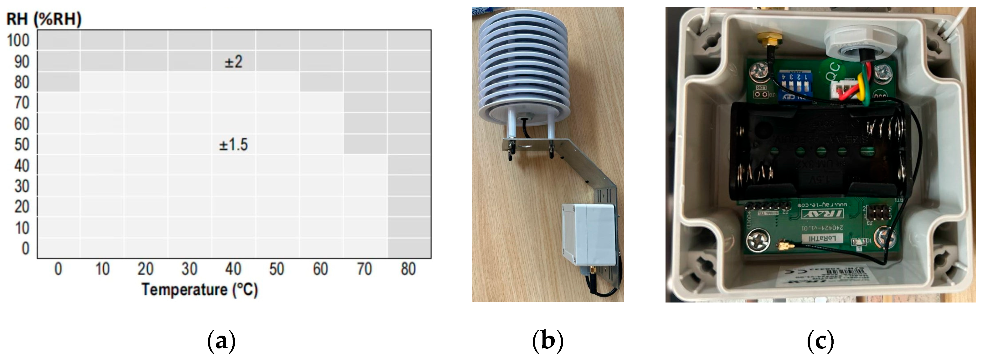
- Sensors
- (b)
- Central processing unit or microcontroller
- Initialization: The measuring functions are included in the base code, and the SHT library is modified to use the SHT35.
- Sampling rate: A default sampling period of 15 min is established, which allows compliance with the Duty Cycle (Air Time) that requires the use of ISM bands, which avoids passing the emissions limit of 1% [68]. This can be modified up to a maximum of one minute if necessary.
- Raw data conversion: The raw data are packaged in a message with the units converted to whole numbers, multiplying the values by 10 to eliminate the decimals. The server later carries out the inverse operation to obtain the decimal value.
- Message coding: To be able to use the LoRaWAN protocol, a series of keywords and addresses have been included that allow the data from the device to be identified and decoded. The ABP method has been used. This programs a Device Address identifier and two keywords (NetworkSessionKey and ApplicationSessionKey) into each AWS that is necessary for connecting to the server that distributes the system’s data, ChirpStack [69].
- Data quality control: This is carried out solely by the SHT35 sensor itself through the basic factory-programmed functions. In addition, although the SHT35 sensor is delivered already calibrated, the various registers of the AWSs have been compared before their definitive installation, placing them in a controlled site for a measurement period of 72 h (the devices registered maximum temperature differences of 0.2 °C and relative humidity differences of 5%, with data being registered every 15 min). On the other hand, as a digital communication bus is used, no loss of accuracy occurs in the data readings.
- Local data storage: Data are temporarily stored in the dynamic memory of the MCU, where the unit conversion takes place and from where the data are sent.
- (c)
- Peripheral equipment
- (d)
- Auxiliary elements
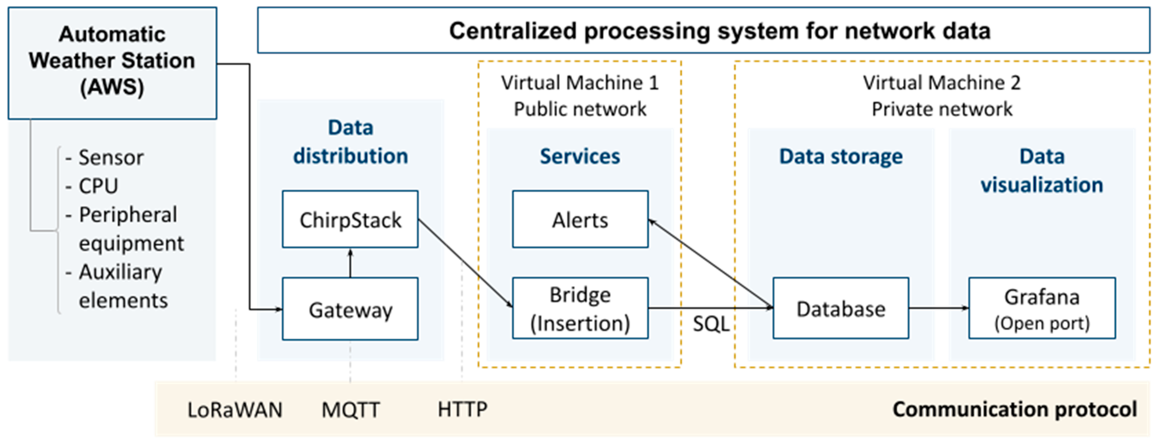
3.2.2. Centralized Processing System for Network Data
- (a)
- Data acquisition and transmission
- Waterproof box for outdoors, the outdoor enclosure model for WisGate Developer D4+ [74]: This box houses the gateway and must have SIM coverage.
- Gateway, RAK WIRELESS 7248C D4H+ model [75]: It consists of a Raspberry Pi processor linked to an RAK2013 Cellular Pi HAT module for connecting to the mobile phone network using a SIM card. It is responsible for receiving and decoding the LoRA packages and sending them to a remote database. It is powered by the electricity grid.
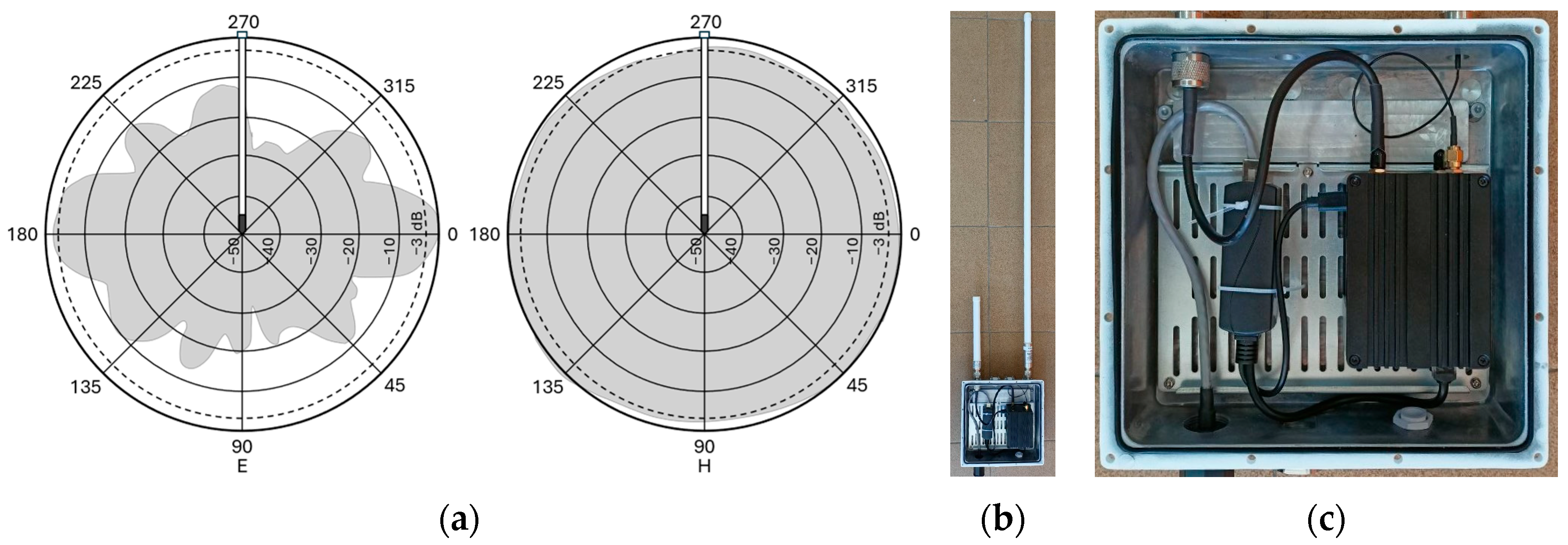
- Omnidirectional LoRa 868 MHz antenna of 8 dBi [76]: This is placed on the upper part of the box and aids in the reception of data packages emitted by the AWSs in the LoRa bandwidth.
- (b)
- Receiving and storing data
- (c)
- Data visualization
3.3. Citizen Weather Observer Networks
3.3.1. Automatic Weather Stations
- (a)
- Sensors, central processing unit, and peripheral equipment
- The sensor used (SHTC3 [80]) measures temperature in a range from −40 °C to 125 °C, with an accuracy of ±0.2 °C, and relative humidity, within a range of 0% to 100%, offering a typical accuracy of ±2%. Measurements have a resolution of 0.01 °C and 0.01%, respectively. Sensors reported LTD ranging from ±0.02 to ±0.04 °C/year. The stations were installed between 2014 and 2024, resulting in accumulated LTD values ranging from ±0.02 °C to ±0.39 °C, depending on the sensor’s age.
- The CPU automatically acquires the data registered by the sensors and then processes and prepares them for internal dispatch. The data transmission between the AWSs and the Nt server is through a Wi-Fi connection that is compatible with the standard 802.11 b/g/n in the frequency band of 2.4 GHz, reinforced with Open, WEP, WPA, and WPA2-personal security protocols. It enables wireless communication via long-range radio between the interior and exterior module, reaching up to 100 m in open field conditions (868 MHz [81]).
- These devices are controlled from a mobile application provided by the manufacturer. It is from this application that the programming is carried out. Many of the operations of the CPU are fixed, programmed from the factory (raw data conversion, local data storage, sampling (five minutes), message coding, and data transmission); as such, it is only necessary to initialize using the internet with a Wi-Fi connection. Once the device has been activated, an initial calibration is automatically executed, and this enables remote diagnostics and maintenance. Similarly, the periodic device updates are carried out automatically.
- Data quality control is carried out in the centralized servers using validation algorithms that compare the data collected from the adjacent AWSs, within the same geographic area, in order to identify atypical values due to faults in the device or to an inadequate installation [82].
- It does not have averaging operations, manual entry of observations, data reduction, or local data visualization.
- As for the peripheral equipment, this device is powered by two AAA batteries with an approximate autonomy of two years for data collection occurring every five minutes. In order to ensure the accuracy of the timings, temporal synchronization mechanisms based on network protocols (such as NTP) are used. Although the manufacturer does not detail the implementation of a clock in real time, the network architecture guarantees that the data from each sensor are coherently integrated in the cloud, allowing precise chronologies [82,83]. Whether the AWSs have specific devices for quality control is not known.
- (b)
- Auxiliary elements
3.3.2. Centralized Network Data Processing System
4. Location and Installation of the Measuring Devices
4.1. Considerations of the WMO
4.1.1. Concerning the Horizontal Scales
4.1.2. Concerning the Vertical Scales
4.2. Bespoke Network
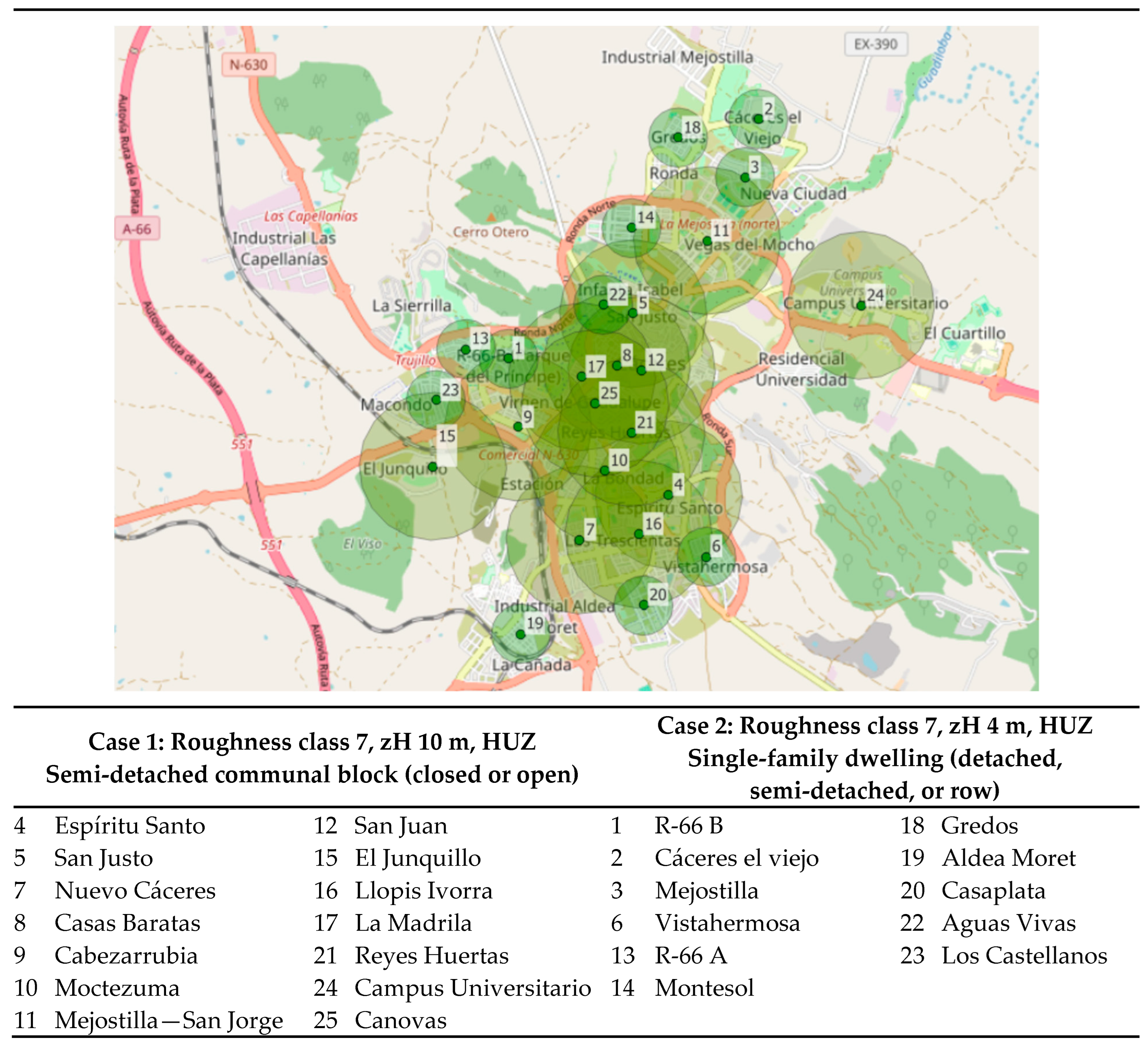
4.2.1. Automatic Weather Stations
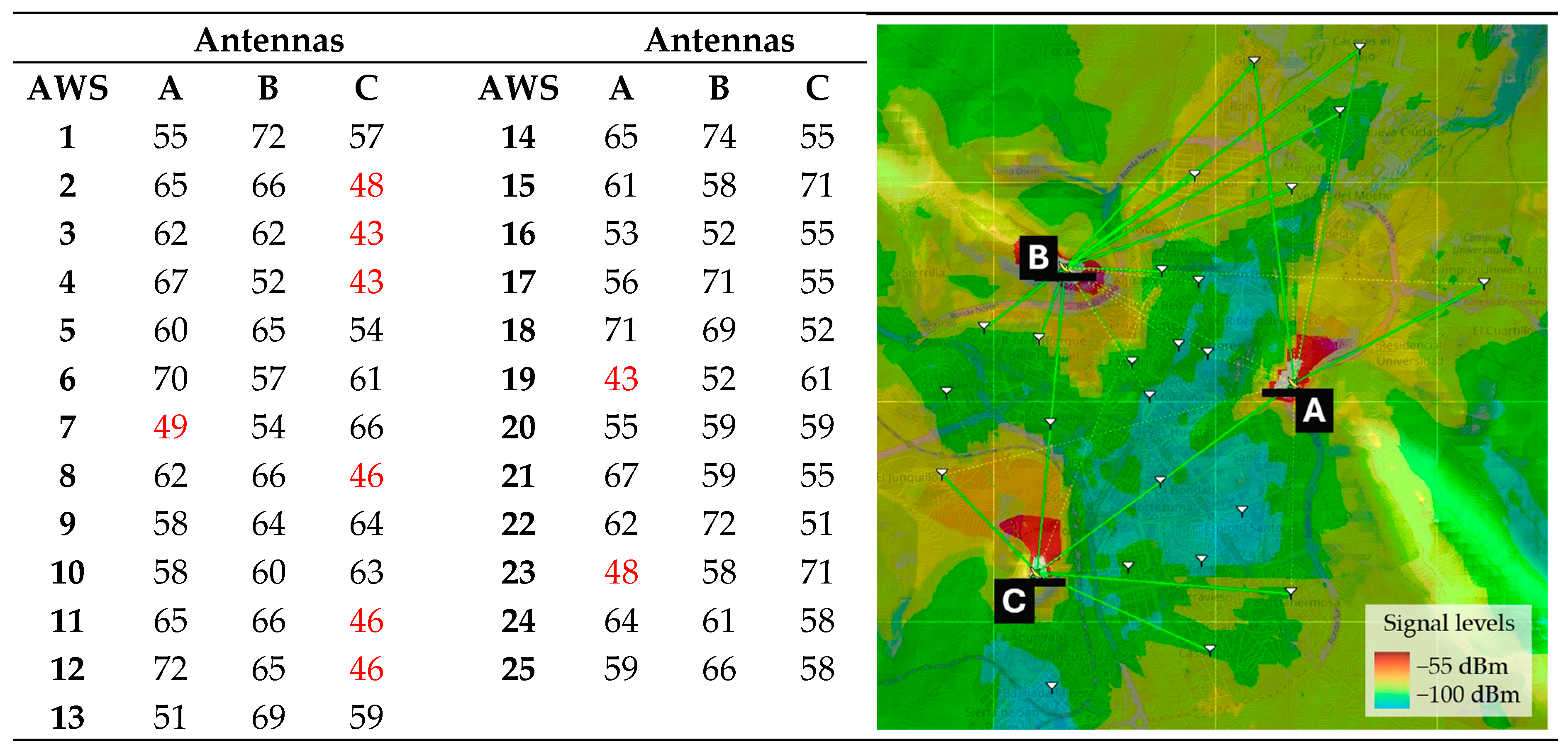
4.2.2. Communication Devices
4.3. Citizen Weather Observer Networks
5. Analysis of the Measurement Data
5.1. Data Quality Control
- Selection of AWSs according to the amount of data, discarding those that do not reach at least 80% (a smaller percentage is considered insufficient to characterize the period).
- Verification of the temperature range for the period in question, which is set from 11 °C to 47 °C (corresponding to ±6 °C with respect to the absolute minimum and maximum temperatures registered by the city’s AEMET station in the month of August 2024, 17 °C and 41 °C, respectively [105]).
- Checking the consistency of the readings for the same value continuously, fixing as outliers those hourly values repeated over 5 consecutive hours.
- Searching for sudden or significant changes between consecutive time marks, defining as outliers those hourly registers with variations above 12 °C with respect to the previous one (to maintain the stability and relevance of the data, ensuring coherent data and eliminating the infrequent sudden changes that are usually due to extreme phenomena or measuring errors).
- Checking the validity of the continuity of the data in between observations and the average of the remaining AWS, fixing a threshold of four standard deviations (guaranteeing the detection of really extreme values, eliminating extremely rare values possibly due to measuring errors or real anomalies, while also minimizing the elimination of legitimate data).
- Checking the daily oscillation in temperatures, eliminating those registers of the days in which the said oscillation is lower than 9 °C (minimum value of thermal oscillation registered by the AEMET in the city in the period in question).
- Checking sensor aging, devices with a total uncertainty exceeding ±0.5 °C were excluded, while those with an accumulated LTD above ±0.3 °C were critically reviewed. As a result, three situations were identified: no evidence of aging in the Bs network; a lack of knowledge for WU network sensors; and a cumulative LTD of ±0.39 °C for devices “h” and “i” in the Nt network; however, these are not associated with any control points or analysis zones, and are therefore of limited relevance to the study.
- The probability distribution and density of the registers from each AWS, according to different temperature ranges (Figure 7): it can be seen that the registers of the AWSs of Bs and WU are uniformly distributed between the different levels, which happens with those of the AEMET, with similar mean values (29.5 ± 0.4 °C in Bs and WU and 29.4 °C in AEMET) and quartiles (first 25.2 ± 0.6 °C and second 34.4 ± 0.6 °C in Bs and WU and 25.2 and 34.5 °C in AEMET). However, those of the Nt show a great heterogeneity (mean 29.5 ± 1.1 °C, first quartile 25.9 ± 1.2 °C, and second quartile 34.8 ± 1.9 °C). The differences between the amplitude of data registered in the AWSs of the different networks are similarly worth noting, while Bs and WU show 3.7 °C (from 20.1 to 23.8 °C) and 6.7 °C (from 19.7 to 26.4 °C), respectively; Nt registers 8.7 °C (from 18.2 to 26.9 °C). On the other hand, the AWS of the AEMET presents an oscillation of 23.1 °C.
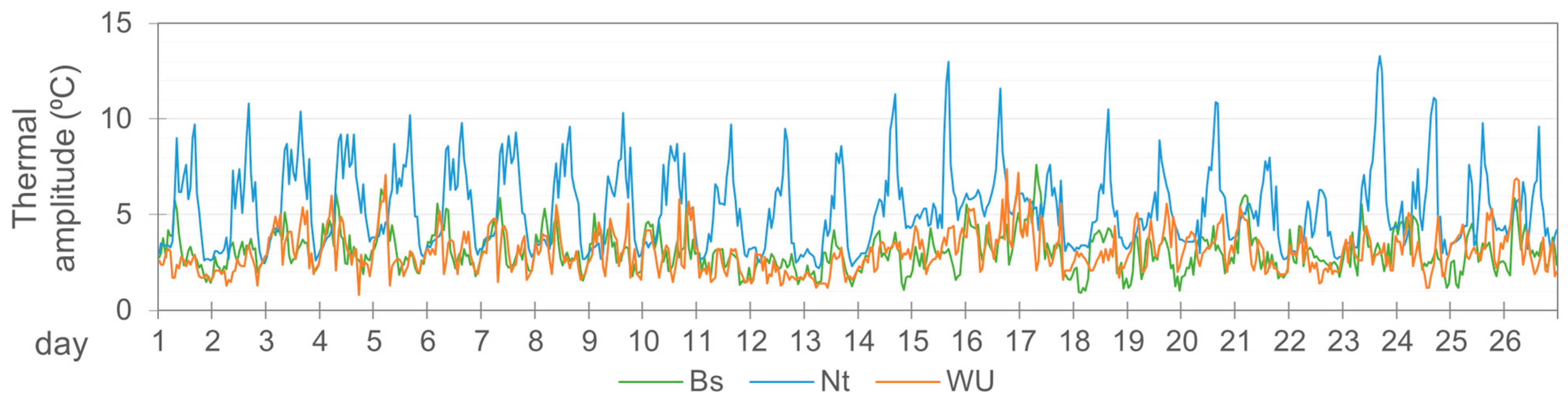
- Hourly differences between the values registered by all the AWSs of each network (Figure 8): Bs and WU have minimums between 0.9 °C and 0.8 °C, and maximums between 7.6 °C and 7.4 °C, respectively; while in Nt, these values are 2.2 °C and 14.0 °C, respectively.
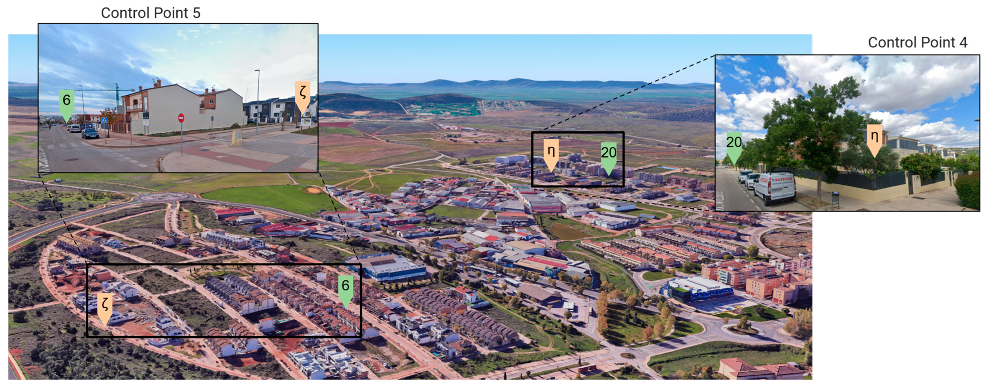
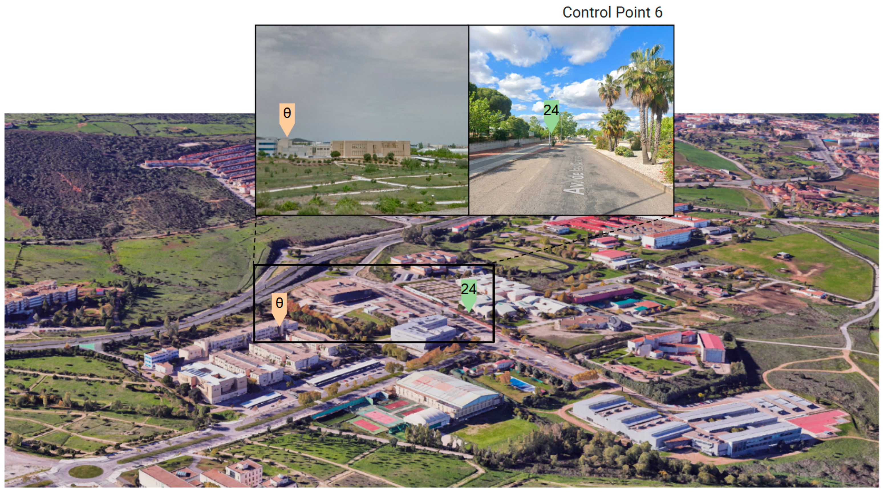
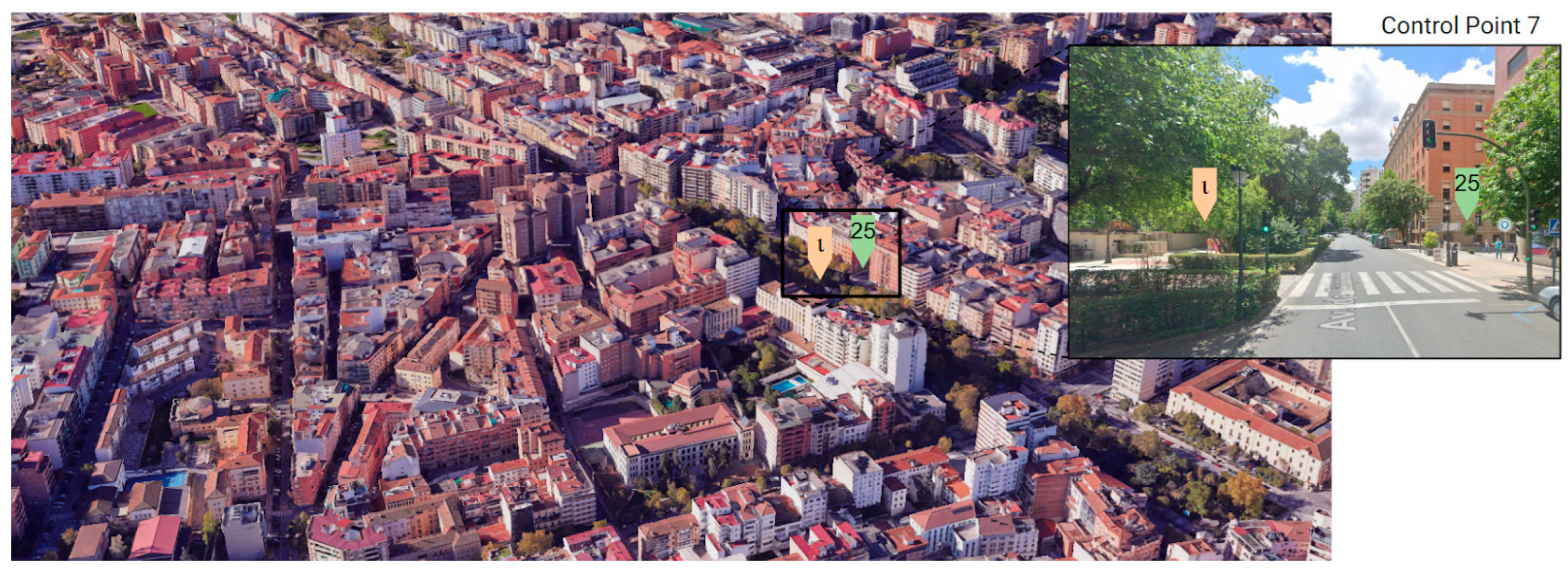
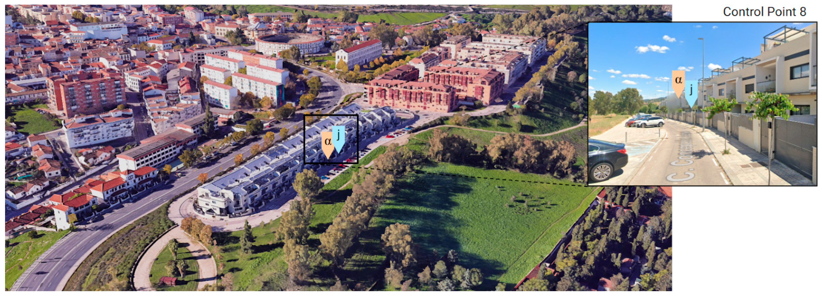
5.2. Control Points
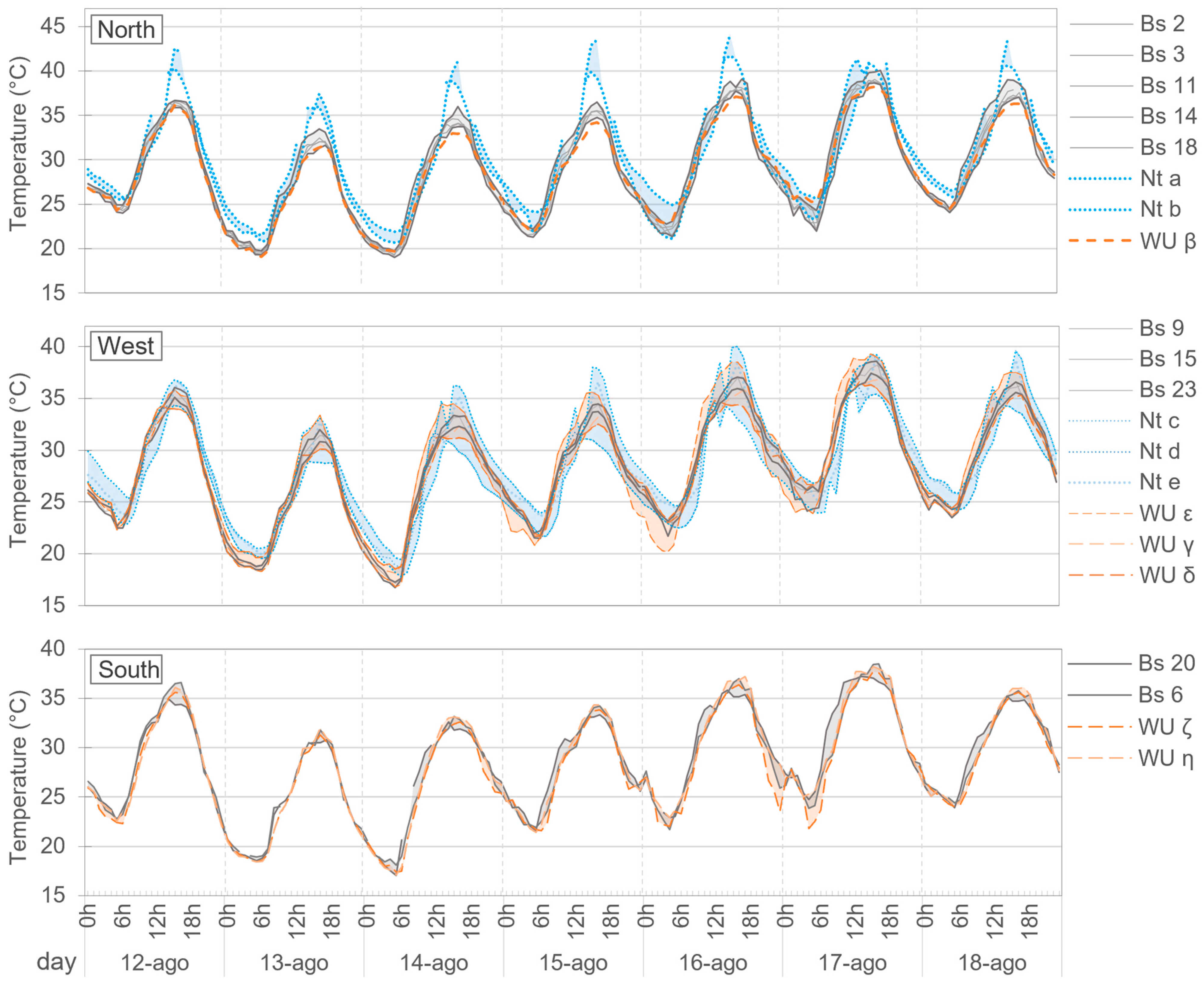
Typical Week
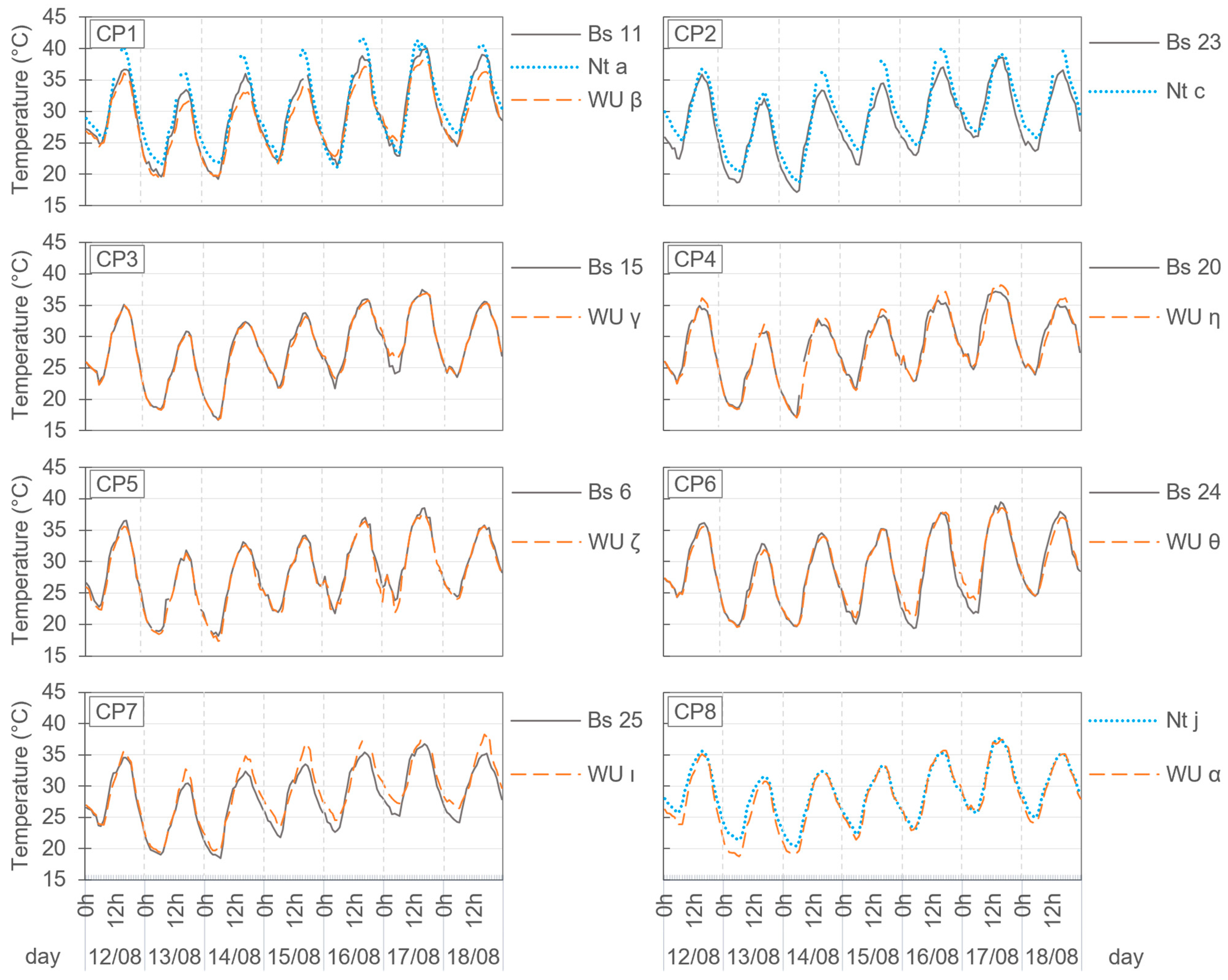
- Similar amplitude with small deviations with respect to the mean, from 0 °C to ±1.0 °C.
- Higher daily registers in the Nt AWSs with respect to the rest, with a mean of 1.6 ± 0.4 °C in the minimum and 2.5 ± 0.4 °C in the maximum with respect to the Bs AWSs, and 1.0 ± 0.2 °C and 2.4 ± 0.3.1 °C, respectively, with respect to the WU AWSs. The differences between the values of the WU and Bs AWSs are small (0.6 ± 0.4 °C in the minimums and 1.1 ± 0.8 °C in the maximums).
- Weekly average greater in the Nt AWSs, with a mean of 1.4 ± 0.1 °C and 1.4 ± 1 °C with respect to the Bs and WU AWSs. There is a mean difference of 0.4 ± 0.3 °C in the weekly average of Bs and WU AWSs.
- A greater average of CDD in the Nt AWSs, with respect to the rest, in totals: 15% and 14% more with respect to the Bs and WU AWS; during daylight: 10% and 9%, respectively; and during the night: 27% and 23%, respectively.

| Control Point and AWS | Weekly Amplitude (°C) | Minimum (°C) | Maximum (°C) | Weekly Average (°C) | CDD (°C·Day) | |||||
|---|---|---|---|---|---|---|---|---|---|---|
| Absolute | Daily Average | Absolute | Daily Average | Totals | Daytime (% of Total) | Nighttime (% of Total) | ||||
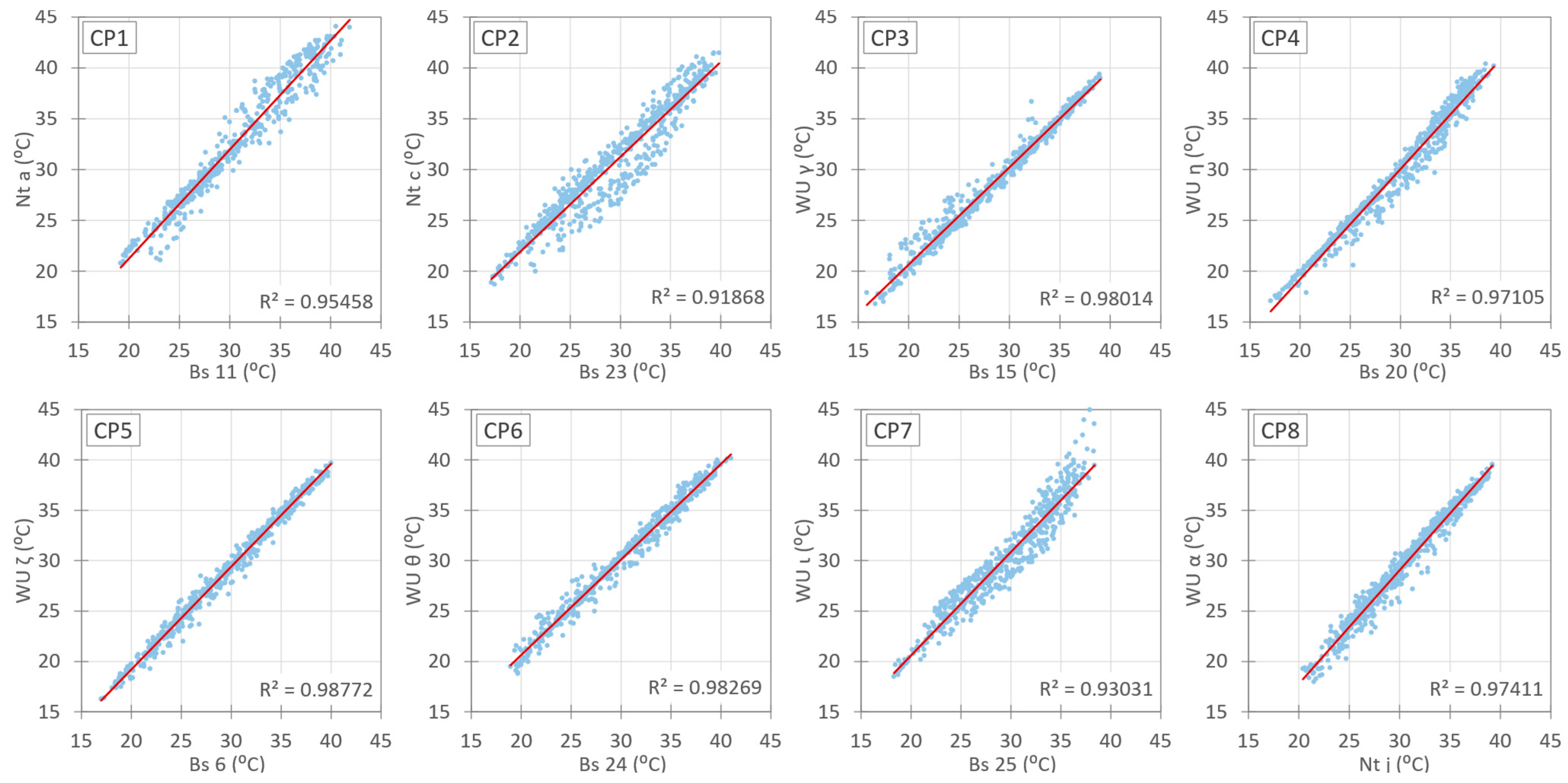
| CP1 | Bs 11 | 20.8 | 19.3 | 21.8 | 40.1 | 37.1 | 29.4 | 141 | 94 (67%) | 46 (33%) |
| Nt a | 20.6 | 21.1 | 23.1 | 41.7 | 39.8 | 30.7 | 169 | 114 (68%) | 55 (32%) | |
| WU β | 19.1 | 19.1 | 22.3 | 38.2 | 35.2 | 28.6 | 141 | 94 (67%) | 47 (33%) | |
| CP2 | Bs 23 | 21.5 | 17.1 | 21.7 | 38.6 | 35.4 | 28.3 | 136 | 93 (69%) | 43 (31%) |
| Nt c | 21.4 | 18.7 | 23.6 | 40.1 | 37.6 | 29.9 | 159 | 101(64%) | 57 (36%) | |
| CP3 | Bs 15 | 20.8 | 16.7 | 21.2 | 37.5 | 34.4 | 28.0 | 133 | 90 (68%) | 43 (32%) |
| WU γ | 20.1 | 16.8 | 21.7 | 36.9 | 34.2 | 28.0 | 138 | 100 (72%) | 38 (28%) | |
| CP4 | Bs 20 | 20.1 | 17.1 | 21.6 | 37.2 | 34.3 | 28.5 | 138 | 95 (68%) | 44 (32%) |
| WU η | 21.1 | 17.1 | 21.6 | 38.2 | 35.3 | 28.4 | 136 | 94 (69%) | 42 (31%) | |
| CP5 | Bs 6 | 20.4 | 18.1 | 21.7 | 38.5 | 35.3 | 28.5 | 136 | 94 (69%) | 43 (31%) |
| WU ζ | 20.3 | 17.4 | 21.1 | 37.7 | 34.7 | 27.9 | 130 | 90 (70%) | 39 (30%) | |
| CP6 | Bs 24 | 20.1 | 19.4 | 21.2 | 39.4 | 36.3 | 28.7 | 140 | 100 (72%) | 40 (28%) |
| WU θ | 18.9 | 19.6 | 21.9 | 38.5 | 35.8 | 28.9 | 143 | 98 (69%) | 45 (31%) | |
| CP7 | Bs 25 | 18.3 | 18.4 | 22.1 | 36.7 | 34.0 | 28.1 | 135 | 90 (67%) | 45 (33%) |
| WU ι | 18.9 | 19.4 | 23.4 | 38.3 | 36.2 | 28.9 | 148 | 93 (63%) | 55 (37%) | |
| CP8 | Nt j | 17.2 | 20.4 | 23.3 | 37.6 | 34.4 | 29.0 | 146 | 94 (65%) | 52 (35%) |
| WU α | 18.6 | 18.8 | 22.1 | 37.4 | 34.2 | 28.2 | 135 | 90 (67%) | 45 (33%) | |
5.3. Control Zones
- The superposition of registers between Bs and WU (mostly in the North and South zones).
- The great similarity between the registers of the AWSs of Bs in each of the three zones (means of 1.6 °C and 0.7 °C in West and South).
- The great difference between the values of the AWSs of WU in the West zone (mean of 1.7 °C and maximum of 4.2 °C).
- The lack of continuity in the registers of the AWSs of Nt (some had to be excluded in the data quality control) and large differences between their registers in the West zone (mean of 2.8 °C and maximum of 7.4 °C), especially in the maximums, which were also very high in the North zone (up to 8.8 °C more than Bs and 9.3 °C more than WU, on August 15th at 16:00 h).
- Large absolute differences between the registers of the AWSs of Nt, with a mean of 2.6 ± 0.7 °C and a maximum of 6.8 ± 0.8 °C. Bs and WU show greater compactness between their AWSs, with a mean of 1 ± 0.4 °C and 1.3 ± 0.9 °C, and a maximum of 3.7 ± 1.4 °C and 4.5 ± 0.4 °C, respectively.
- A similar amplitude (mean of the AWS) between the networks of the West and South zones, while in the North zone, the Nt measures 2.9 °C and 3.7 °C more with respect to the Bs and WU, respectively.
- Larger daily maximum and minimum registers in Nt with respect to Bs and WU, with a mean of 1.4 ± 0.3 °C and 1.2 ± 0.1 °C more in the minimums and 2.9 ± 2.9 °C and 3.6 ± 3.4 °C more in the maximums, respectively. Small differences between Bs and WU, of 0.8 ± 1.0 °C in the minimums and 0.5 ± 0.5 °C in the maximums.
- Weekly average larger in Nt with respect to Bs and WU, with 1.1 ± 1.0 °C and 1.2 ± 1.2 °C more on average, respectively. Mean difference of 0.2 ± 0.2 °C between Bs and WU.
- Similar daytime and nighttime totals for CDD in Bs and WU (difference of 2%). Larger values in Nt with respect to Bs and WU, over 6 °C and 8 °C·day, respectively, in the daytime and approximately 10 °C·day at night. This supposes an increase with respect to Bs and WU of 8 ± 8% and 11 ± 12% in the daytime and 23 ± 4% and 21 ± 0% at night, respectively.
- A similar share between daytime and nighttime CDD, with respect to the total, in all three networks, around 68% and 32%.
| No. of AWSs per Network | Between AWSs of Each Network: Absolute Difference (°C) | Between Networks | ||||||||
|---|---|---|---|---|---|---|---|---|---|---|
| Weekly Amplitude (°C) | Average Daily Values (°C) | Weekly Average (°C) | CDD (°C·Day) | |||||||
| Totals | Daytime (% of Total) | Nighttime (% of Total) | ||||||||
| Max | Average | Min | Max | |||||||
| North zone | ||||||||||
| Bs | 5 | 4.7 | 1.5 | 19.9 | 21.9 | 36.3 | 28.9 | 143 | 98 (69%) | 45 (31%) |
| Nt | 2 | 6.2 | 2.0 | 22.8 | 23.5 | 41.2 | 30.7 | 168 | 112 (67%) | 56 (33%) |
| WU * | 1 | - | - | 19.1 | 22.3 | 35.2 | 28.6 | 141 | 94 (67%) | 47 (33%) |
| West zone | ||||||||||
| Bs | 3 | 2.1 | 0.8 | 21.1 | 21.6 | 35.0 | 28.3 | 135 | 92 (68%) | 43 (32%) |
| Nt | 3 | 7.4 | 3.1 | 20.1 | 22.8 | 35.9 | 28.6 | 142 | 90 (63%) | 52 (37%) |
| WU | 3 | 4.2 | 2.0 | 20.2 | 21.7 | 34.7 | 28.2 | 135 | 92 (68%) | 43 (32%) |
| South zone | ||||||||||
| Bs | 2 | 4.2 | 0.8 | 20.3 | 21.6 | 34.8 | 28.5 | 137 | 94 (69%) | 43 (31%) |
| Nt | 0 | |||||||||
| WU | 2 | 4.8 | 0.7 | 20.7 | 23.5 | 35.0 | 28.1 | 133 | 92 (69%) | 41 (31%) |
6. Discussion of Results
6.1. Concerning the Choice of Components and Programming of the System
6.2. Concerning the Location and Installation of Measuring Devices
6.3. Concerning the Analysis of Measurement Data
7. Conclusions
Author Contributions
Funding
Institutional Review Board Statement
Informed Consent Statement
Data Availability Statement
Conflicts of Interest
Correction Statement
Abbreviations
| ABP | Activation By Personalization |
| ABS | Acrylonitrile Butadiene Styrene |
| API | Application Programming Interface |
| AWS | Automatic Weather Station |
| Bs | Bespoke network |
| CDD | Cooling Degree Days |
| CP | Control Point |
| CPU | Central Processing Unit |
| CWON | Citizen Weather Observer Networks |
| CWS | Citizen Weather Station |
| HTTP | Hypertext Transfer Protocol |
| HUZ | Homogeneus Urban Zone |
| ID | Identification |
| IDE | Integrated Development Environment |
| IoT | Internet of Things |
| IPCC | Intergovernmental Panel on Climate Change |
| ISM bands | Industrial, Scientific and Medical bands |
| LCZ | Local Climate Zones |
| MCU | Microcontroller Unit |
| MQTT | Message Queuing Telemetry Transport |
| NMHS | National Meteorological and Hydrological Services |
| Nt | Netatmo network |
| NTP | Network Time Protocol |
| RF | Radio Frequency |
| RTC | Real-Time Clock |
| RTD | Real-Time Data |
| SNR | Signal-Noise Ratio |
| SQL | Structured Query Language |
| SUHI | Surface Urban Heat Island |
| UCL | Urban Canopy Layer |
| UCZ | Urban Climate Zone |
| UHI | Urban Heat Island |
| USB | Universal Serial Bus |
| VM | Virtual Machine |
| WMO | World Meteorological Organization |
| WU | Weather Underground network |
| LTD | Long-term drift |
Appendix A
| Brand and Model | Physical Specifications | Type: Parameters (Range/Accuracy/Precision)//Sampling Rate/Polling Rate | CPU Functions | Data Transmission | Peripheral Equipment |
|---|---|---|---|---|---|
| RainWise MK4-C Compact Cellular Weather Station (Boothwyn, PA, USA) | 28 × 58 × 91 cm 4 kg Highly durable materials | Basic: temperature (Range: −40 to 60 °C/Accuracy ±0.25 °C/Resolution 0.1 °C), relative humidity (Range: 0 to 100%/Accuracy ±1.5% (from 0 to 80%)/resolution 1%), precipitation, atmospheric pressure and wind.//Records every 1 min. Displays every 15 min | Factory CPU. Includes factory averaging: Records every minute. The reported value is the average of the 15 min logs. Highs and lows are based on 1 min readings. Activation required: Activating Data Plan and Registering Online via their website using the RainWise MK4-C MAC address and serial number. | Data transmission via SIM/LTE connectivity, supporting CAT/LTE-M and NB-IoT cellular networks. Data are sent every 15 min. | 1. Solar Panel mono crystaline 7 V 2.3 W + Battery Non-Spillable 4 V 4.5 Ah AGM sealed lead-acid 1A peak, 12 mA typical. Battery Life: 2 to 5 years typical |
| RainWise PWS Direct to Weather Underground (Boothwyn, PA, USA) | Equivalent characteristics in terms of dimensions, materials and sensors. | Basic: temperature, relative humidity, precipitation, atmospheric pressure, wind, and dew point temperature. No capability to add additional sensors to this station.//Real-time data updates up to 3 s | Based on the same hardware platform as the MK4-C. Preprogrammed WU-100 interface for direct connection to the Weather Underground® personal weather station (PWS) network. Optimized for seamless integration with the WU network | WiFi/Network Interface IP-100: Gateway to the Internet; enables unprecedented transmission and access to real-time weather data through multiple formats. Storage and forwarding capabilities. | Solar-powered with backup battery. |
| Davis VantageVue Package (Hayward, CA, USA, EEUU) | 33 × 34 × 15 cm 3 kg UV-resistant ABS and ASA plastic | Basic: Temperature (Range: −40 to 65 °C/Accuracy: ±0.3 °C), relative humidity (Range: 0 to 100%/Accuracy: ±2%), precipitation, atmospheric pressure, and wind. Type: Temperature: Silicon diode with PN junction/Relative humidity: Film capacitor.//Real-time data updates every 2.5 s. | Integrated CPU in the WeatherLink Console. It is responsible for receiving, processing, and converting into digital format the signals coming from the external sensors of the Sensor Suite. It also performs internal calculations to generate derived parameters such as heat index, dew point, barometric trends, and weather forecasts, which can then be displayed on the console screen. It acts as the core that manages the WeatherLink Console’s user interface, enabling data visualization through tabs (such as “Current Weather”, “Graph”, “Data”, and “Map”), and facilitating connection to online services for data publishing and storage. Additionally, it handles system settings, including alarms and calibration. | WiFi. Complemented by devices such as AirBridge or WeatherBridge. | Solar panel (5 watts) + built-in supercapacitor. Backup lithium battery (3-volt CR-123 lithium cell) with a lifespan of 8 months to 2 years. |
| Ambient Weather WS-2902B (Chandler, AZ, USA) | 38 × 28 × 25.5 cm | Extended: temperature (Range: −40 to 65 °C/Accuracy ±2 °C/Resolution 0.1 °C), relative humidity (Range: 10 to 99%/Accuracy ±5%/resolution 1%), precipitation, atmospheric pressure, wind and solar radiation and UV.//Records every 5 min | It receives the analog signals from the sensors and converts them into digital data that can be processed. Then, it applies calibration algorithms to correct the measurements. Additionally, it runs the internal software that coordinates the station’s operation, controlling aspects such as time synchronization, screen updating, alarm management, and executing calibration and reset functions. | WiFi (Sensor Array RF Frequency: 915 MHz. WiFi Console RF Frequency: 2.4 GHz) | Solar + supercapacitor. Backup battery (3 AAA batteries) |
| Bloomsky Weather Station (Burlingame, CA, USA) | 33 × 20 × 18 cm 1 kg | Extended: temperature (Range: −20 to 55 °C/Accuracy: ±0.3 °C), relative humidity (Range: 0 to 100%/Accuracy: ±3% (from 10 to 90%)), precipitation, atmospheric pressure, wind, UV radiation, and real-time camera. Type: thermometer, hygrometer.//Records every 5 min | It collects the signals from the various connected sensors and processes them to generate readings of the meteorological variables. Then, it stores data and performs internal calculations to obtain derived parameters, according to what is configured by the user or preset in the firmware. It also manages communication and controls system functions. | WiFi. Weather data and real-time images are transmitted by the built in WiFi module at regular intervals throughout the day. | Solar option. AC and Battery (1 Lithium Ion battery) |
| AcuRite 5-in- 1 Weather Environment System ((Chaney Instrument Co.) Lake Geneva, WI, USA) | 35 × 27.5 × 14 cm 1.8 kg | Basic: 5-in-1 sensor: temperature (Range: −40 to 70 °C/Accuracy: ±1 °C), relative humidity (Range: 1 to 99%), precipitation, atmospheric pressure, and wind. It features an internally powered aspirating fan, powered by a solar panel.//Records every 5 min | Storage of 8760 records. | WiFi. Communicates via a 433 MHz signal. | Solar + backup batteries (4 AA lithium batteries) (providing up to 12 h of operation during a power outage) |
| La Crosse Professional Weather Station (La Crosse, WI, USA) | 20 × 15 × 4 cm 400 gr Durable plastic | Basic: temperature (Range: −40 to 60 °C/Accuracy: ±0.5 °C), relative humidity (Range: 10 to 99%), precipitation, atmospheric pressure, and wind. Type: LTV-TH5i sensor (temp and RH) and LTV-WSDR1 sensor (others).//Records every 5 min | - | WiFi. Frecuencia de transmisión: 915 MHz | Solar and Battery Powered (LTV-TH5i sensor: 2 AA alkaline batteries and LTV-WSDR1: 3 AA alkaline batteries). Battery life: 2 years. |
| Netatmo Weather Station (Boulogne-Billancourt, France) | Indoor module: 45 × 45 × 155 mm Outdoor module: 45 × 45 × 105 mm Anodized aluminum | Light: indoor temperature (Range: 0 to 50 °C/Accuracy: ±0.3 °C), outdoor temperature (Range: −40 to 65 °C/Accuracy: ±0.3 °C), relative humidity (Range: 0% to 100%/Accuracy: ±3%), barometric pressure, CO2.//Records every 5 min | Data processing: receives measurements from the integrated sensors and processes them to generate understandable data. Communication management: controls the transmission of data between modules and ensures connection to the home Wi-Fi network to send information to Netatmo’s servers. Temporary storage: maintains temporary records of the measurements before transmission, ensuring data integrity in case of connection interruptions. | Data transmission between accessory modules and the main module is performed via a low-power wireless connection. Data transmission to the Netatmo server: Wi-Fi—The main module connects to the home Wi-Fi network using the 2.4 GHz band. The station is not compatible with networks operating exclusively on the 5 GHz band. | Indoor module: USB power adapter. Outdoor module: 2 AAA batteries, with a lifespan of up to 2 years. |
Appendix B
| Control Points | (% Records) | Distance Between AWSs (m) | District | ||
|---|---|---|---|---|---|
| AWS Bs | AWS Nt | AWS WU | |||
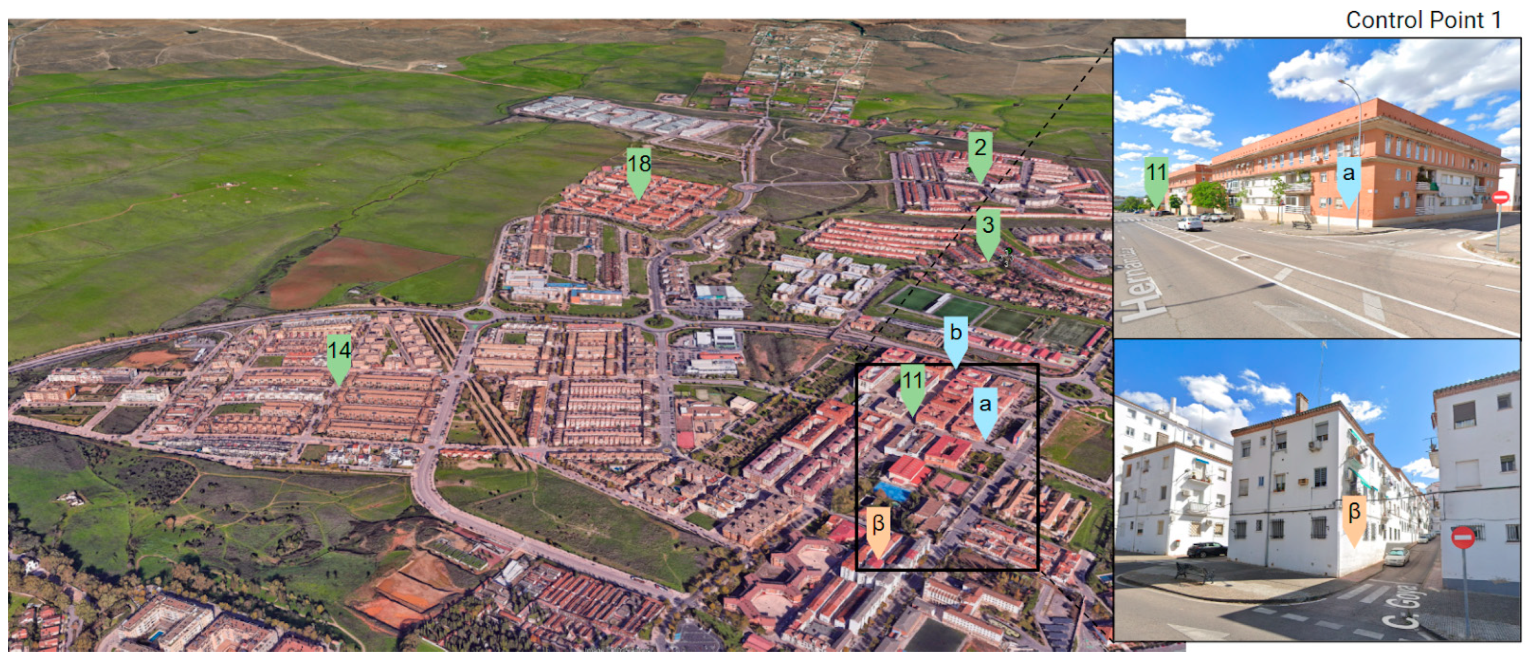
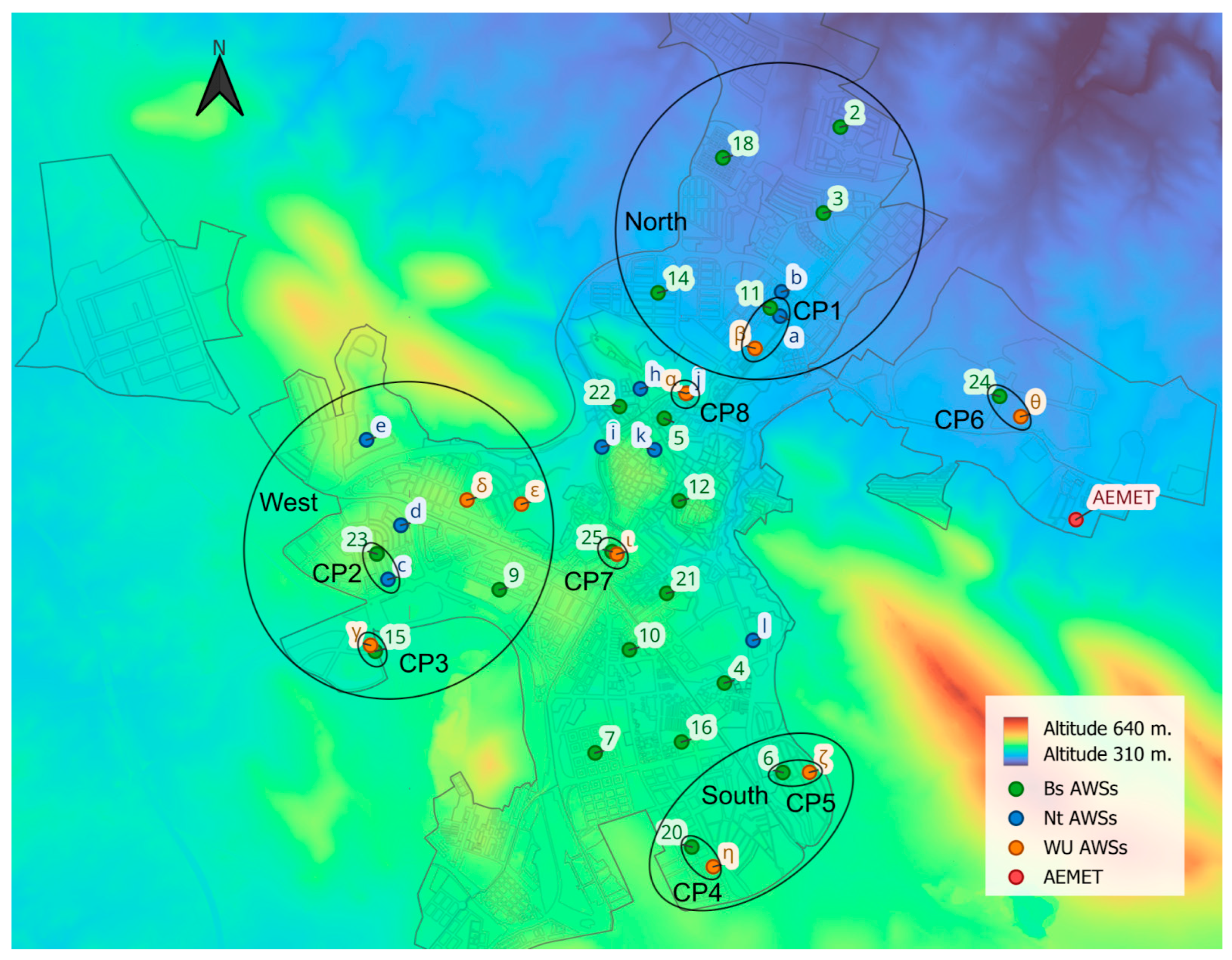
| CP1 | 11 (100%) | a (81%) | β (100%) | 100/300 | Mejostilla/San Jorge |
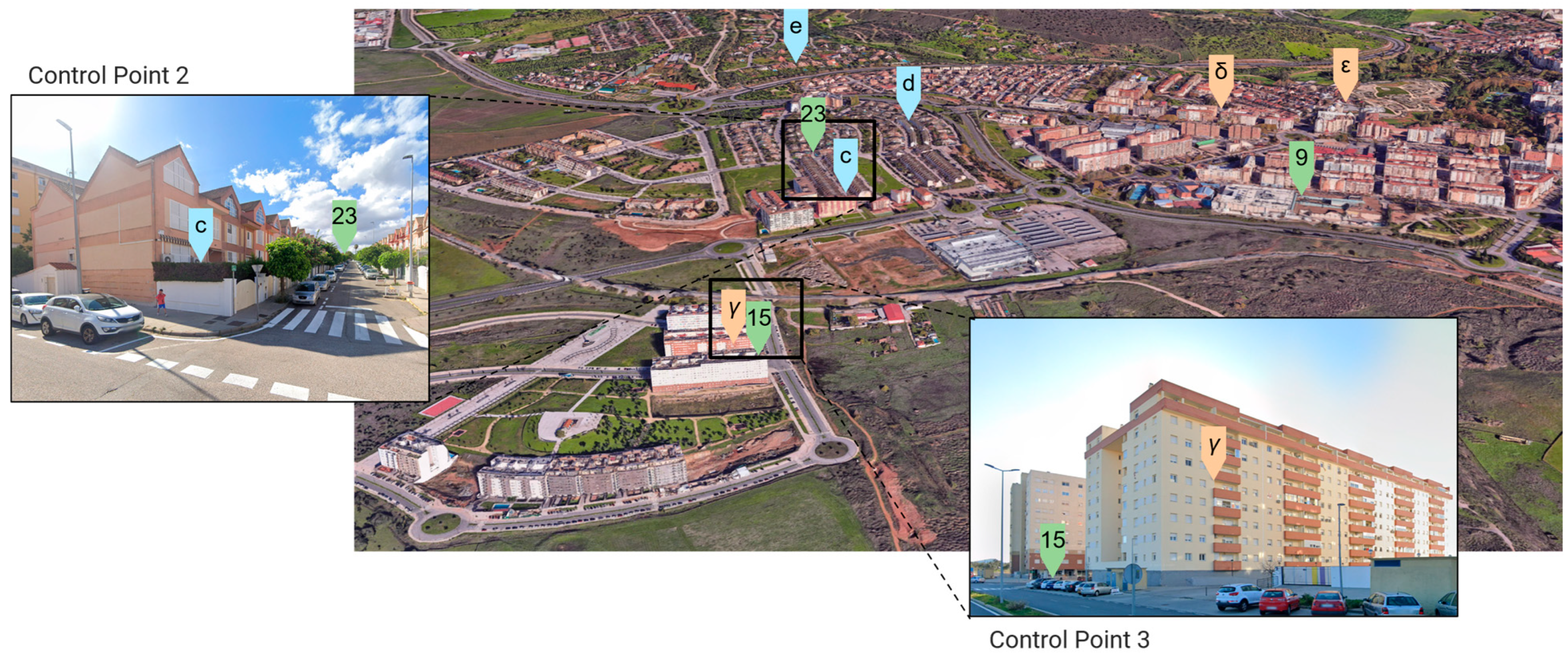
| CP2 | 23 (100%) | c (100%) | - | 250 | Los Castellanos |
| CP3 | 15 (100%) | - | γ (100%) | 60 | Junquillo |
| CP4 | 20 (98%) | - | η (100%) | 215 | Casaplata |
| CP5 | 6 (89%) | - | ζ (100%) | 200 | Vistahermosa |
| CP6 | 24 (100%) | - | θ (100%) | 250 | Campus universitario |
| CP7 | 25 (100%) | - | ι (99%) | 40 | Cánovas |
| CP8 | - | j (100%) | α (100%) | 20 | Infanta Isabel |
| North Zone | West Zone | South Zone | |
|---|---|---|---|
| Elevation (Altitude) (m) | 40 (from 350 to 390) | 35 (from 350 to 385) | 25 (from 440 to 465) |
| Extension (Ha) | 294 | 176 | 77 |
| District | Cáceres el Viejo, Montesol, Mejostilla, Gredos and San Jorge | El Junquillo, La Sierrilla, Los Castellanos and Cabezarrubia | Vistahermosa and Casa Plata |
| Open areas or green zones | No large wooded areas on non-urban edges and no green areas within neighborhoods | Large green areas nearby both on non-urban edges and in the inner urban area | Unbuilt urbanized areas, with extensive surrounding crop areas |
| HUZ | Terraced and row houses and Semi-Open Collective (from 1 to 4 floors high) | ||
| Construction date | 1995–2010 | 1995–2010 | 2002–present |
| Number of AWSs (Bs/Nt/WU) | 8 units (2, 3, 11, 14, 18/a, b/β) | 9 units (9, 15, 23/c, d, e/γ, δ, ε) | 4 units (6, 20/ζ, η) |
| % records | 99% | 100% | 99% |
Appendix C
References
- United Nations. Department of Economic and Social Affairs, Population Division, World Urbanization Prospects. The 2018 Revision, New York. 2018. Available online: https://population.un.org/wup/publications (accessed on 10 April 2025).
- UN-Habitat, European Commission. Healthier Cities and Communities Through Public Spaces. 2025. Available online: https://unhabitat.org/healthier-cities-and-communities-through-public-spaces (accessed on 10 April 2025).
- Olaniyi, O.O.; Okunleye, O.J.; Olabanji, S.O. Advancing Data-Driven Decision-Making in Smart Cities through Big Data Analytics: A Comprehensive Review of Existing Literature. Curr. J. Appl. Sci. Technol. 2023, 42, 10–18. [Google Scholar] [CrossRef]
- Cities, A.S. Open & Agile Smart Cities & Communities (OASC). 2025. Available online: https://oascities.org/ (accessed on 10 April 2025).
- Centre for Urban Transformation, G20 Global Smart Cities Alliance. 2025. Available online: https://www.globalsmartcitiesalliance.org/home (accessed on 10 April 2025).
- Organisation for Economic Co-operation and Development, Organization for Economic Co-operation and Development (OECD). 2025. Available online: https://www.oecd.org/en/about/programmes/the-oecd-programme-on-smart-cities-and-inclusive-growth0.html (accessed on 10 April 2025).
- Governance of the Living-in.EU Community (Go Li.EU), Smart Communities Network. 2025. Available online: https://living-in.eu/eu-support-services/smart-communities-network (accessed on 10 April 2025).
- Müller-Eie, D.; Kosmidis, I. Sustainable mobility in smart cities: A document study of mobility initiatives of mid-sized Nordic smart cities. Eur. Transp. Res. Rev. 2023, 15, 36. [Google Scholar] [CrossRef]
- Szpilko, D.; de la Torre Gallegos, A.; Naharro, F.J.; Rzepka, A.; Remiszewska, A. Waste Management in the Smart City: Current Practices and Future Directions. Resources 2023, 12, 115. [Google Scholar] [CrossRef]
- Mohammadzadeh, Z.; Saeidnia, H.R.; Lotfata, A.; Hassanzadeh, M.; Ghiasi, N. Smart city healthcare delivery innovations: A systematic review of essential technologies and indicators for developing nations. BMC Health Serv. Res. 2023, 23, 1180. [Google Scholar] [CrossRef] [PubMed]
- Ullo, S.L.; Sinha, G.R. Advances in Smart Environment Monitoring Systems Using IoT and Sensors. Sensors 2020, 20, 3113. [Google Scholar] [CrossRef]
- Faraji, A.; Rashidi, M.; Rezaei, F.; Rahnamayiezekavat, P. A Meta-Synthesis Review of Occupant Comfort Assessment in Buildings (2002–2022). Sustainability 2023, 15, 4303. [Google Scholar] [CrossRef]
- Biennial of Public Space, United Nations Programme on Human Settlements (UN-Habitat), Charter of Public Space. 2016. Available online: https://habnet.unhabitat.org/sites/default/files/documents/Charter%20of%20Public%20Space.pdf (accessed on 10 April 2025).
- The Intergovernmental Panel on Climate Change (IPCC), The Intergovernmental Panel on Climate Change (IPCC). 2025. Available online: www.ipcc.ch/ (accessed on 10 April 2025).
- Afaq, H.; Chambers, D.N.; Zolnikov, T.R. Urban Heat Islands. The Palgrave Encyclopedia of Urban and Regional Futures. In The Palgrave Encyclopedia of Urban and Regional Futures; Springer International Publishing: Cham, Switzerland, 2022; pp. 1–7. [Google Scholar] [CrossRef]
- Nuruzzaman, M.; Island, U.H. Effects and Mitigation Measures—A Review. Int. J. Environ. Monit. Anal. 2015, 3, 67. [Google Scholar] [CrossRef]
- Mentaschi, L.; Duveiller, G.; Zulian, G.; Corbane, C.; Pesaresi, M.; Maes, J.; Stocchino, A.; Feyen, L. Global long-term mapping of surface temperature shows intensified intra-city urban heat island extremes. Glob. Environ. Change 2022, 72, 102441. [Google Scholar] [CrossRef]
- Wandl, A.; van der Hoeven, F. Amsterwarm: Mapping the landuse, health and energy-efficiency implications of the Amsterdam urban heat island. Build. Serv. Eng. Res. Technol. 2015, 36, 67–88. [Google Scholar] [CrossRef]
- Icaza, L.E.; van der Hoeven, F.D.; van den Dobbelsteen, A. The Urban Heat Island Effect in Dutch City Centres: Identifying Relevant Indicators and First Explorations. In Implementing Climate Change Adaptation in Cities and Communities; Springer: Cham, Switzerland, 2016; pp. 123–160. [Google Scholar] [CrossRef]
- Morris, K.I.; Salleh, S.A.; Chan, A.; Ooi, M.C.G.; Abakr, Y.A.; Oozeer, M.Y.; Duda, M. Computational study of urban heat island of Putrajaya, Malaysia. Sustain. Cities Soc. 2015, 19, 359–372. [Google Scholar] [CrossRef]
- Ichim, P.; Sfîcă, L.; Kadhim-Abid, A. Characteristics of Nocturnal Urban Heat Island of Iaşi During a Summer Heat Wave (1–6 August 2017). In Aerul şi Apa: Componente ale Mediului; Cluj University Press: Cluj-Napoca, Romania, 2018; pp. 253–260. [Google Scholar] [CrossRef]
- Garau, G.A.; Garau, J.L. The urban heat island in Palma (Majorca, Balearic islands): Progress in the study of urban climate in a Mediterranean coastal city. Bol. Asoc. Geografos Espanoles 2018, 2018, 392–418. [Google Scholar] [CrossRef]
- World Meteorological Organization, WMO, n.d. Available online: https://wmo.int/es (accessed on 10 April 2025).
- World Meteorological Organization (WMO). Guide to Instruments and Methods of Observation (Volume I—Measurement of Meteorological Variables, Volume II—Measurement of Cryospheric Variables, Volume III—Observing Systems, Volume IV—Space-Based Observations and Volume V—Quality Assurance and Management of Observing Systems), 2023 ed.; World Meteorological Organization: Geneva, Switzerland, 2023. [Google Scholar]
- Peng, S.; Piao, S.; Ciais, P.; Friedlingstein, P.; Ottle, C.; Bréon, F.-M.; Nan, H.; Zhou, L.; Myneni, R.B. Surface Urban Heat Island Across 419 Global Big Cities. Environ. Sci. Technol. 2012, 46, 696–703. [Google Scholar] [CrossRef] [PubMed]
- MODIS Moderate Resolution Imaging Spectoradiometer, (n.d.). Available online: https://modis.gsfc.nasa.gov/ (accessed on 10 April 2025).
- NASA/USGS, Landsat Science. 2025. Available online: http://landsat.gsfc.nasa.gov/ (accessed on 10 April 2025).
- Agencia Espacial Europea, Sentinel. 2025. Available online: http://sentinels.copernicus.eu/ (accessed on 10 April 2025).
- Weng, Q. Thermal infrared remote sensing for urban climate and environmental studies: Methods, applications, and trends. ISPRS J. Photogramm. Remote Sens. 2009, 64, 335–344. [Google Scholar] [CrossRef]
- Ma, L.; Zhu, X.; Qiu, C.; Blaschke, T.; Li, M. Advances of Local Climate Zone Mapping and Its Practice Using Object-Based Image Analysis. Atmosphere 2021, 12, 1146. [Google Scholar] [CrossRef]
- Wang, C.; Bi, X.; Luan, Q.; Li, Z. Estimation of Daily and Instantaneous Near-Surface Air Temperature from MODIS Data Using Machine Learning Methods in the Jingjinji Area of China. Remote Sens. 2022, 14, 1916. [Google Scholar] [CrossRef]
- Steinbeis Europa Zentrum, Smart Cities Marketplace. 2025. Available online: www.steinbeis-europa.de/en/projects/smart-cites-marketplace-2-0 (accessed on 10 April 2025).
- EURO CITIES, Smart Cities Information System. 2025. Available online: http://eurocities.eu/projects/smart-cities-information-system/ (accessed on 10 April 2025).
- Eumetnet, Eumetnet. 2025. Available online: www.eumetnet.eu/ (accessed on 10 April 2025).
- Hahn, C.; Garcia-Marti, I.; Sugier, J.; Emsley, F.; Beaulant, A.-L.; Oram, L.; Strandberg, E.; Lindgren, E.; Sunter, M.; Ziska, F. Observations from Personal Weather Stations—EUMETNET Interests and Experience. Climate 2022, 10, 192. [Google Scholar] [CrossRef]
- Golroudbary, V.R.; Zeng, Y.; Mannaerts, C.M.; Su, Z. Urban impacts on air temperature and precipitation over The Netherlands. Clim. Res. 2018, 75, 95–109. [Google Scholar] [CrossRef]
- Chapman, L.; Bell, C.; Bell, S. Can the crowdsourcing data paradigm take atmospheric science to a new level? A case study of the urban heat island of London quantified using Netatmo weather stations. Int. J. Climatol. 2017, 37, 3597–3605. [Google Scholar] [CrossRef]
- Meier, F.; Fenner, D.; Grassmann, T.; Otto, M.; Scherer, D. Crowdsourcing air temperature from citizen weather stations for urban climate research. Urban. Clim. 2017, 19, 170–191. [Google Scholar] [CrossRef]
- Feichtinger, M.; de Wit, R.; Goldenits, G.; Kolejka, T.; Hollósi, B.; Žuvela-Aloise, M.; Feigl, J. Case-study of neighborhood-scale summertime urban air temperature for the City of Vienna using crowd-sourced data. Urban. Clim. 2020, 32, 100597. [Google Scholar] [CrossRef]
- de Vos, L.W.; Droste, A.M.; Zander, M.J.; Overeem, A.; Leijnse, H.; Heusinkveld, B.G.; Steeneveld, G.J.; Uijlenhoet, R. Hydrometeorological Monitoring Using Opportunistic Sensing Networks in the Amsterdam Metropolitan Area. Bull. Am. Meteorol. Soc. 2020, 101, E167–E185. [Google Scholar] [CrossRef]
- Napoly, A.; Grassmann, T.; Meier, F.; Fenner, D. Development and Application of a Statistically-Based Quality Control for Crowdsourced Air Temperature Data. Front. Earth Sci. 2018, 6, 00118. [Google Scholar] [CrossRef]
- Sun, C.-Y.; Kato, S.; Gou, Z. Application of Low-Cost Sensors for Urban Heat Island Assessment: A Case Study in Taiwan. Sustainability 2019, 11, 2759. [Google Scholar] [CrossRef]
- Martinez-Soto, A.; Vera-Fonseca, M.; Valenzuela-Toledo, P.; Melillan-Raguileo, A.; Shupler, M. Heat on the Move: Contrasting Mobile and Fixed Insights into Temuco’s Urban Heat Islands. Sensors 2025, 25, 1251. [Google Scholar] [CrossRef]
- Battista, G.; Evangelisti, L.; Guattari, C.; De Cristo, E.; De Lieto Vollaro, R.; Asdrubali, F. An Extensive Study of the Urban Heat Island Phenomenon in Rome, Italy: Implications for Building Energy Performance Through Data from Multiple Meteorological Stations. Int. J. Sustain. Dev. Plan. 2023, 18, 3357–3362. [Google Scholar] [CrossRef]
- Husni, E.; Prayoga, G.A.; Tamba, J.D.; Retnowati, Y.; Fauzandi, F.I.; Yusuf, R.; Yahya, B.N. Microclimate investigation of vehicular traffic on the urban heat island through IoT-Based device. Heliyon 2022, 8, e11739. [Google Scholar] [CrossRef]
- Ma, D.; Brousse, O.; De Jode, M.; Hudson-Smith, A. Using Bespoke LoRaWAN Heat Sensors to Explore Microclimate Effects within the London Urban Heat Islands-A Pilot Study in East London. In Proceedings of the 32nd Annual GIS Research UK Conference (GISRUK), Leeds, UK, 9–12 April 2024. [Google Scholar] [CrossRef]
- Chapman, L.; Muller, C.L.; Young, D.T.; Warren, E.L.; Grimmond, C.S.B.; Cai, X.-M.; Ferranti, E.J.S. The Birmingham Urban Climate Laboratory: An Open Meteorological Test Bed and Challenges of the Smart City. Bull. Am. Meteorol. Soc. 2015, 96, 1545–1560. [Google Scholar] [CrossRef]
- Martín-Garín, A.; Millán-García, J.A.; Hernández-Minguillón, R.J.; Prieto, M.M.; Alilat, N.; Baïri, A. Open-Source Framework Based on LoRaWAN IoT Technology for Building Monitoring and Its Integration into BIM Models. In Handbook of Smart Materials, Technologies, and Devices; Springer International Publishing: Cham, Switzerland, 2022; pp. 257–283. [Google Scholar] [CrossRef]
- Ma, M.; Bartocci, E.; Lifland, E.; Stankovic, J.A.; Feng, L. A Novel Spatial–Temporal Specification-Based Monitoring System for Smart Cities. IEEE Internet Things J. 2021, 8, 11793–11806. [Google Scholar] [CrossRef]
- Bell, S.; Cornford, D.; Bastin, L. How good are citizen weather stations? Addressing a biased opinion. Weather 2015, 70, 75–84. [Google Scholar] [CrossRef]
- Oke, T.E. Initial Guidance to Obtain Representative Meteorological Observations at Urban Sites. 2006. Available online: https://urban-climate.org/wp-content/uploads/2023/10/Oke_2006_IOM-81-UrbanMetObs.pdf (accessed on 10 April 2025).
- Instituto Nacional de Estadística (INE), Cifras Oficiales de Población de los Municipios Españoles en Aplicación de la Ley de Bases del Régimen Local (Art. 17). 2025. Available online: www.ine.es/jaxiT3/Datos.htm?t=2863 (accessed on 10 April 2025).
- Sánchez-Guevara, C.; Arrieta, L.G.; Pozas, B.M. OLADAPT: Olas de calor y ciudades: Adaptación y resiliencia del entorno construido, Ministerio de Ciencia, Innovación y Universidades PID2022-138284OA-C32. 2023. [Google Scholar]
- Netatmo, Netatmo Weather. 2025. Available online: www.netatmo.com/weather-with-netatmo (accessed on 10 April 2025).
- Coney, J.; Pickering, B.; Dufton, D.; Lukach, M.; Brooks, B.; Neely, R.R. How useful are crowdsourced air temperature observations? An assessment of Netatmo stations and quality control schemes over the United Kingdom. Meteorol. Appl. 2022, 29, e2075. [Google Scholar] [CrossRef]
- The Weather Company, Weather Underground. 2025. Available online: https://www.wunderground.com/ (accessed on 10 April 2025).
- Meteoclimatic, Meteoclimatic. 2025. Available online: www.meteoclimatic.net/mapinfo/ESEXT?screen_width=2560 (accessed on 10 April 2025).
- Noromet, Noromet Asociación Meteorológica del Noroeste Peninsular. 2025. Available online: https://noromet.org/ (accessed on 10 April 2025).
- NCEI National Centers for Environmental Information, NCEI National Centers for Environmental Information. 2025. Available online: www.ncei.noaa.gov/ (accessed on 10 April 2025).
- Organización Meteorológica Mundial, Guía de Instrumentos y Métodos de Observación Meteorológicos. 2014. Available online: www.wmo.int (accessed on 10 April 2025).
- Sánchez-Sánchez, F.A.; Vega-De-Lille, M.; Castillo-Atoche, A.A.; López-Maldonado, J.T.; Cruz-Fernandez, M.; Camacho-Pérez, E.; Rodríguez-Reséndiz, J. Geo-Sensing-Based Analysis of Urban Heat Island in the Metropolitan Area of Merida. Mexico. Sensors 2024, 24, 6289. [Google Scholar] [CrossRef] [PubMed]
- Mathew, A.; Aljohani, T.H.; Shekar, P.R.; Arunab, K.S.; Sharma, A.K.; Ahmed, M.F.M.; Idris, U.I.A.; Almohamad, H.; Abdo, H.G. Spatiotemporal dynamics of urban heat island effect and air pollution in Bengaluru and Hyderabad: Implications for sustainable urban development. Discov. Sustain. 2025, 6, 134. [Google Scholar] [CrossRef]
- Martín-Garín, A.; Millán-García, J.A.; Baïri, A.; Gabilondo, M.; Rodríguez, A. IoT and cloud computing for building energy efficiency. In Start-Up Creation; Elsevier: Amsterdam, The Netherlands, 2020; pp. 235–265. [Google Scholar] [CrossRef]
- iRay Electronic Engineering, iRay Electronic Engineering. 2025. Available online: https://ray-ie.com/ (accessed on 10 April 2025).
- T.S.C. Sensirion, Datasheet SHT3x-DIS. 2022. Available online: https://sensirion.com/ (accessed on 10 April 2025).
- GitHub, MCU ATMega328P. 2025. Available online: https://github.com/raymirabel/LoRaTH (accessed on 10 April 2025).
- DigiKey, 2J0C15-868-C885G 868 MHz ISM Connector Mount, DigiKey. 2025. Available online: https://www.digikey.es/es/products/detail/2j-antennas/2J0C15-868-C885G/22108775?srsltid=AfmBOorQJKnMrtUYXOKnezqCeCbtP6lyFCDOWMEuLBIVJtCs9TXUghbo (accessed on 10 April 2025).
- ETSI, EN 300 220-2–V3.2.1–Short Range Devices (SRD) Operating in the Frequency Range 25 MHz to 1 000 MHz; Part 2: Harmonised Standard for Access to Radio Spectrum for Non Specific Radio Equipment. 2018. Available online: https://portal.etsi.org/TB/ETSIDeliverableStatus.aspx (accessed on 10 April 2025).
- ChirpStack; ChirpStack, Servidor de Red LoRaWAN. 2025. Available online: www.chirpstack.Io/ (accessed on 10 April 2025).
- BricoGeek, Adafruit RFM95W LoRa Radio (900 Mhz). 2025. Available online: https://tienda.bricogeek.com/lora/1097-adafruit-rfm95w-lora-radio-900-mhz.html (accessed on 10 April 2025).
- LoRa Alliance®, The Things Network. 2025. Available online: https://www.thethingsnetwork.org/docs/lorawan/regional-parameters/eu868/ (accessed on 10 April 2025).
- JEDEC. Global Standards for the Microelectronics Industry, Standards & Documents. 2025. Available online: https://www.jedec.org/document_search?search_api_views_fulltext=JESD47 (accessed on 10 April 2025).
- RIKA Sensor, RK95-01 Protector Solar Multiplaca. 2025. Available online: https://www.rikasensor.com/rk95-01-multi-plate-ambient-weather-radiation-shield.html (accessed on 10 April 2025).
- RAK, Outdoor Enclosure for WisGate Developer Gateway. 2025. Available online: https://store.rakwireless.com/products/outdoor-enclosure-kit-h?srsltid=AfmBOopTK3Lstjr8Z-xBoMTZYVVnQFxFDnaLxYDzX9DsJZ87mqOEmvyy&variant=37912840634566 (accessed on 10 April 2025).
- Maker Store, RAK Wireless 7248C WisGate Developer D4H+ (con LTE). 2025. Available online: https://maker-store.es/iot-lora-nb-iot-rfid-m2m-co/lora/lora-gateways/7058/rak-wireless-7248c-wisgate-developer-d4h-con-lte (accessed on 10 April 2025).
- S-Connect, Antenna ISM/LoRA Barracuda OMB.868.B08F21 868MHz 8dBi Omnidirectional Outdoor Wall/Pole Mount N-Type(F). 2025. Available online: https://s-connect.es/Antenna-ISM-LoRA-Barracuda-OMB.868.B08F21-868MHz-8dBi-Omnidirectional-Outdoor-Wall-Pole-Mount-N-Type-F/OMB.868.B08F21 (accessed on 10 April 2025).
- Telegram, Telegram. 2025. Available online: https://telegram.org/ (accessed on 10 April 2025).
- Grafana Labs, Grafana. 2025. Available online: https://grafana.com/ (accessed on 10 April 2025).
- Weather Underground, Personal Weather Station Buying Guide. 2025. Available online: https://www.wunderground.com/pws/buying-guide (accessed on 10 April 2025).
- T.S.C. Sensirion, Datasheet SHTC3. 2022. Available online: https://sensirion.com/media/documents/643F9C8E/63A5A436/Datasheet_SHTC3.pdf (accessed on 10 April 2025).
- Netatmo, Avec la Station Météo Intelligente, Mesurez Précisément Votre Environnement. 2025. Available online: www.netatmo.com/fr-fr/smart-weather-station (accessed on 10 April 2025).
- Netatmo, Weather Guide. 2025. Available online: www.netatmo.com/es-es/weather-guide/ (accessed on 10 April 2025).
- Netatmo, Estación Meteorológica Netatmo: Análisis Completo. 2025. Available online: https://estaciondemeteorologia.com/estacion-meteorologica-netatmo/ (accessed on 10 April 2025).
- Weather Underground, Personal Weather Station Network. 2025. Available online: https://www.wunderground.com/pws/about (accessed on 10 April 2025).
- Mideycontrola.com, Estaciones Meteorológicas. 2025. Available online: https://mideycontrola.com/estaciones-meteorologicas (accessed on 10 April 2025).
- AcuRite, AcuRite Iris (5-in-1) Weather Station. 2025. Available online: www.acurite.com/collections/iris/products/acurite-iris-5-in-1-weather-station-with-wi-fi-connection-to-weather-underground (accessed on 10 April 2025).
- Netatmo, Weather API Documentation. 2025. Available online: https://dev.netatmo.com/apidocumentation/weather (accessed on 10 April 2025).
- Netatmo, MeatherMap Netatmo. 2025. Available online: https://weathermap.netatmo.com/ (accessed on 10 April 2025).
- Ambient Weather AirBridge for Davis Weather Stations Quick Start Guide. 2014. Available online: https://www.meteobridge.com/wiki/index.php?title=Home (accessed on 10 April 2025).
- Ambient Weather, AirBridge Download Center. 2025. Available online: http://ambientweather.com/faqs/question/view/id/2477/ (accessed on 10 April 2025).
- Ambient Weather, The WeatherBridge. 2025. Available online: https://ambientweather.com/blog/weatherbridge-easily-connect-davis-acurite-fine-offset-tempest-station-ambientweather (accessed on 10 April 2025).
- Weather Underground, WunderMap. 2025. Available online: https://www.wunderground.com/wundermap (accessed on 10 April 2025).
- Weather Underground, Weather Apps. 2025. Available online: https://www.wunderground.com/download (accessed on 10 April 2025).
- Davenport, A.G. Rationale for Determining Design Wind Velocities. 1960. Available online: https://ascelibrary.org/doi/10.1061/JSDEAG.0000521 (accessed on 10 April 2025).
- Radio Mobile, Radio Mobile–Software de Simulación de Propagación de RF. 2025. Available online: http://radiomobile.pe1mew.nl/ (accessed on 10 April 2025).
- MeteoEstacion—Estaciones Meteorológicas & Meteorología, Consejos y Recomendaciones en la INSTALACIÓN de estaciones Meteorológicas para Lograr Datos de Calidad. 2025. Available online: http://estaciondemeteorologia.com/recomendaciones-instalacion-estaciones-meteorologicas-datos-calidad/ (accessed on 10 April 2025).
- Weather Underground, Installing Your Personal Weather Station. 2025. Available online: https://www.wunderground.com/pws/installation-guide (accessed on 10 April 2025).
- Topographic-map.com, Mapa Topográfico Cáceres. 2025. Available online: https://es-es.topographic-map.com/map-6943l/C%C3%A1ceres/?center=39.46993%2C-6.39462&zoom=15&popup=39.46407%2C-6.39896 (accessed on 10 April 2025).
- Ministerio para la Transición Ecológica y el Reto Demográfico, AEMET. Agencia Estatal de Meteorología. 2025. Available online: www.aemet.es/es/portada (accessed on 10 April 2025).
- American National Standards Institute, ANSI/ASHRAE Standard 55-2020. Thermal Environmental Conditions for Human Occupancy. 2020. Available online: https://www.ashrae.org/technical-resources/bookstore/standard-55-thermal-environmental-conditions-for-human-occupancy (accessed on 10 April 2025).
- Barrao, S.; Serrano-Notivoli, R.; Cuadrat, J.M.; Tejedor, E.; Sánchez, M.A.S. Characterization of the UHI in Zaragoza (Spain) using a quality-controlled hourly sensor-based urban climate network. Urban. Clim. 2022, 44, 101207. [Google Scholar] [CrossRef]
- Beck, C.; Straub, A.; Breitner, S.; Cyrys, J.; Philipp, A.; Rathmann, J.; Schneider, A.; Wolf, K.; Jacobeit, J. Air temperature characteristics of local climate zones in the Augsburg urban area (Bavaria, southern Germany) under varying synoptic conditions. Urban. Clim. 2018, 25, 152–166. [Google Scholar] [CrossRef]
- Fenner, D.; Bechtel, B.; Demuzere, M.; Kittner, J.; Meier, F. CrowdQC+—A Quality-Control for Crowdsourced Air-Temperature Observations Enabling World-Wide Urban Climate Applications. Front. Environ. Sci. 2021, 9, 720747. [Google Scholar] [CrossRef]
- Medina, D.C.; Delgado, M.G.; Ramos, J.S.; Amores, T.P.; Rodríguez, L.R.; Domínguez, S.Á. Empowering urban climate resilience and adaptation: Crowdsourcing weather citizen stations-enhanced temperature prediction. Sustain. Cities Soc. 2024, 101, 105208. [Google Scholar] [CrossRef]
- AEMET. Agencia Estatal de Meteorología, Analisis Estacional. Cáceres. 2025. Available online: www.aemet.es/es/serviciosclimaticos/vigilancia_clima/analisis_estacional?w=2&l=3469A&datos=temp (accessed on 10 April 2025).


| Bs | Nt | WU | ||
|---|---|---|---|---|
| Uniformity of devices | Yes | Partially | No | |
| Uniformity of device locations | Partially | No | No | |
| Sensor’s characteristics | *1 | |||
| Temperature range | Partially | Partially | Partially | |
| Temperature accuracy | Partially | Partially | No | |
| Temperature resolution | Yes | Yes | Yes | |
| Relative humidity range | Yes | Yes | Yes | |
| Relative humidity accuracy | No | No | No | |
| Relative humidity resolution | Yes | Yes | Yes | |
| Rugged, low-maintenance, and minimally distorted | Yes | Yes | *1 | |
| Air temperature control elements | ||||
| Radiation screen | Yes | - | - *1 | |
| Ventilated radiation screens | Yes | Yes | *1 | |
| Forced ventilation | No | No | *1 | |
| Materials and thermal conductivity | Yes | Yes | *1 | |
| Diameter and height | No | No | *1 | |
| Sampling frequency and accuracy | *1 | |||
| Minimum sampling interval | Yes | Yes | Yes *1 | |
| Local storage or preferred RTD | Yes | Yes | Yes | |
| Prioritizing automatic stations with respect to manual stations | Yes | Yes | Yes | |
| Height and location of sensors | ||||
| Sensor height | Yes | - | - | |
| Proximity and distance to obstacles | Yes | - | - | |
| Location with representative HUZ | Yes | Partially | Partially | |
| Calibration and quality control | ||||
| Sensors periodic calibration in laboratory or on-site | *2 | - | - | |
| Reporting of the periodic calibrations | *2 | No | No | |
| Automatic quality control | Verification of data: continuity, stability and consistency | Partially | Partially | Partially |
| Comparison with nearby stations | No | Yes | Yes | |
| Metadata | GPS coordinates and altitude | Yes | No | No |
| Environmental characteristics | Yes | No | No | |
| Sensor type and model | Yes | Yes | No | |
| Installation date | Yes | No | No | |
| Maintenance | Yes | No | No | |
Disclaimer/Publisher’s Note: The statements, opinions and data contained in all publications are solely those of the individual author(s) and contributor(s) and not of MDPI and/or the editor(s). MDPI and/or the editor(s) disclaim responsibility for any injury to people or property resulting from any ideas, methods, instructions or products referred to in the content. |
© 2025 by the authors. Licensee MDPI, Basel, Switzerland. This article is an open access article distributed under the terms and conditions of the Creative Commons Attribution (CC BY) license (https://creativecommons.org/licenses/by/4.0/).
Share and Cite
Lucas Bonilla, M.; Albalá Pedrera, I.T.; Bustos García de Castro, P.; Martín-Garín, A.; Montalbán Pozas, B. Comparing Monitoring Networks to Assess Urban Heat Islands in Smart Cities. Appl. Sci. 2025, 15, 6100. https://doi.org/10.3390/app15116100
Lucas Bonilla M, Albalá Pedrera IT, Bustos García de Castro P, Martín-Garín A, Montalbán Pozas B. Comparing Monitoring Networks to Assess Urban Heat Islands in Smart Cities. Applied Sciences. 2025; 15(11):6100. https://doi.org/10.3390/app15116100
Chicago/Turabian StyleLucas Bonilla, Marta, Ignacio Tadeo Albalá Pedrera, Pablo Bustos García de Castro, Alexander Martín-Garín, and Beatriz Montalbán Pozas. 2025. "Comparing Monitoring Networks to Assess Urban Heat Islands in Smart Cities" Applied Sciences 15, no. 11: 6100. https://doi.org/10.3390/app15116100
APA StyleLucas Bonilla, M., Albalá Pedrera, I. T., Bustos García de Castro, P., Martín-Garín, A., & Montalbán Pozas, B. (2025). Comparing Monitoring Networks to Assess Urban Heat Islands in Smart Cities. Applied Sciences, 15(11), 6100. https://doi.org/10.3390/app15116100