Figure 1.
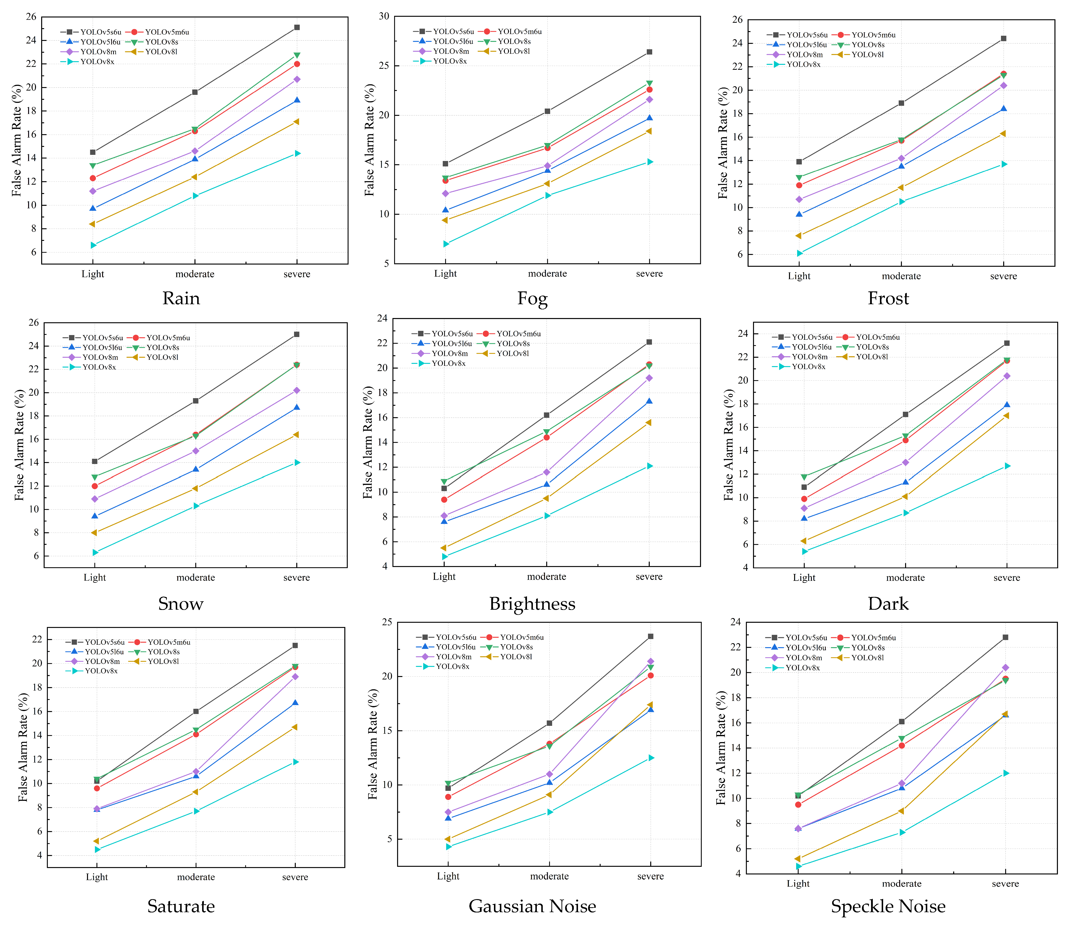
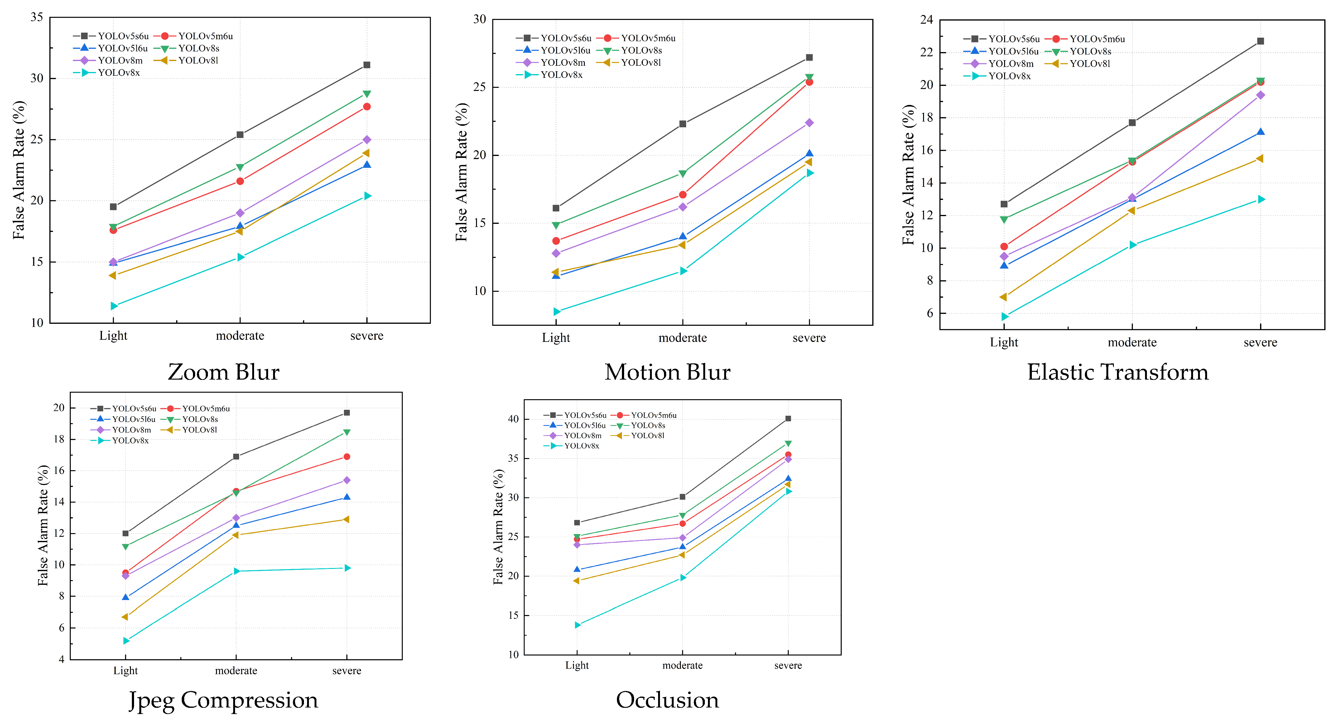
There are 14 types of corruption that can affect 2D vehicle detection, categorized into four categories: weather, color, noise, and blur, transform.
Figure 1.
There are 14 types of corruption that can affect 2D vehicle detection, categorized into four categories: weather, color, noise, and blur, transform.
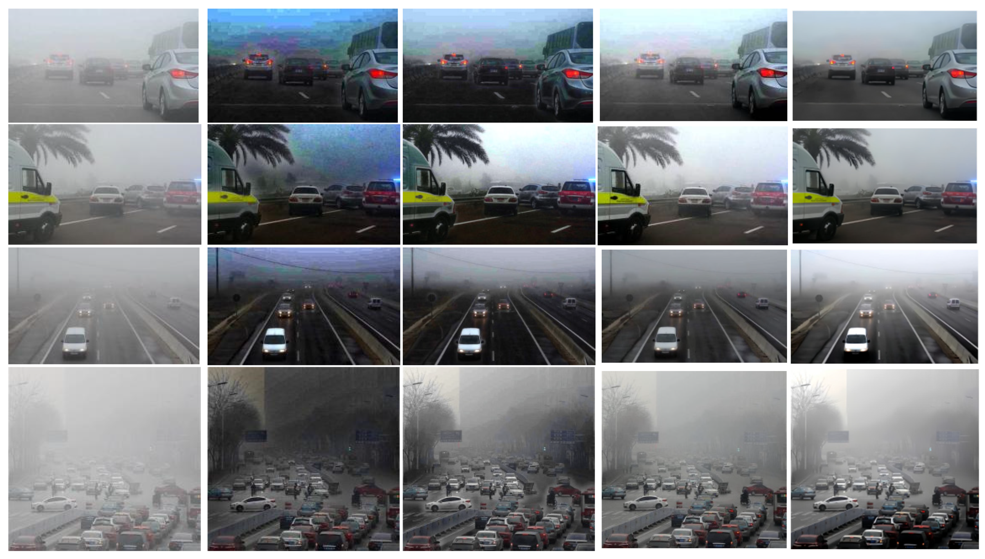
Figure 2.
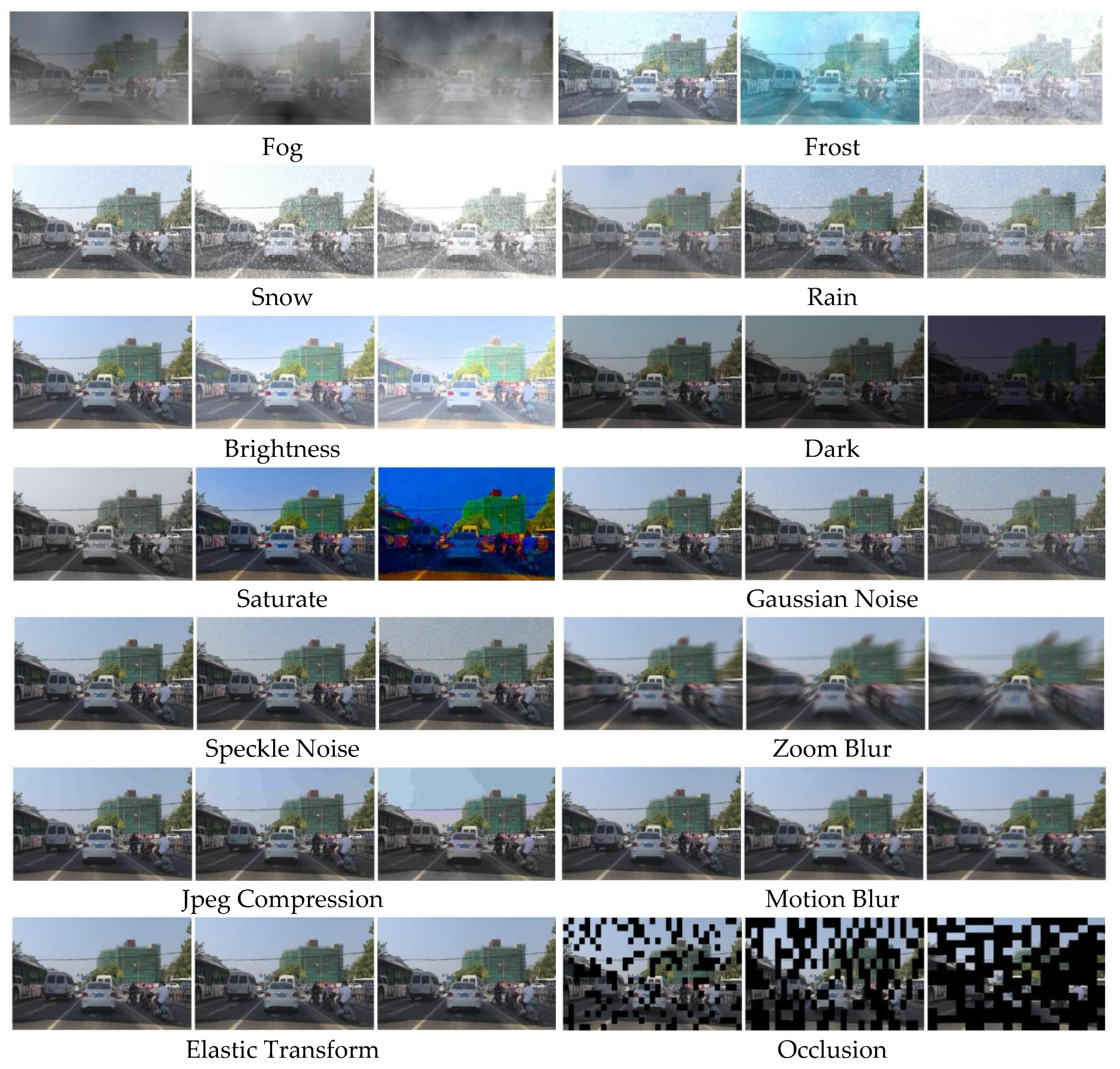
Visualization of three levels of 14 kinds of corruption corresponding to each image.
Figure 2.
Visualization of three levels of 14 kinds of corruption corresponding to each image.
Figure 3.
4 kinds of corruption types of real adverse weather.
Figure 3.
4 kinds of corruption types of real adverse weather.
Figure 4.
Restoration results by SDM under different text prompts.
Figure 4.
Restoration results by SDM under different text prompts.
Figure 5.
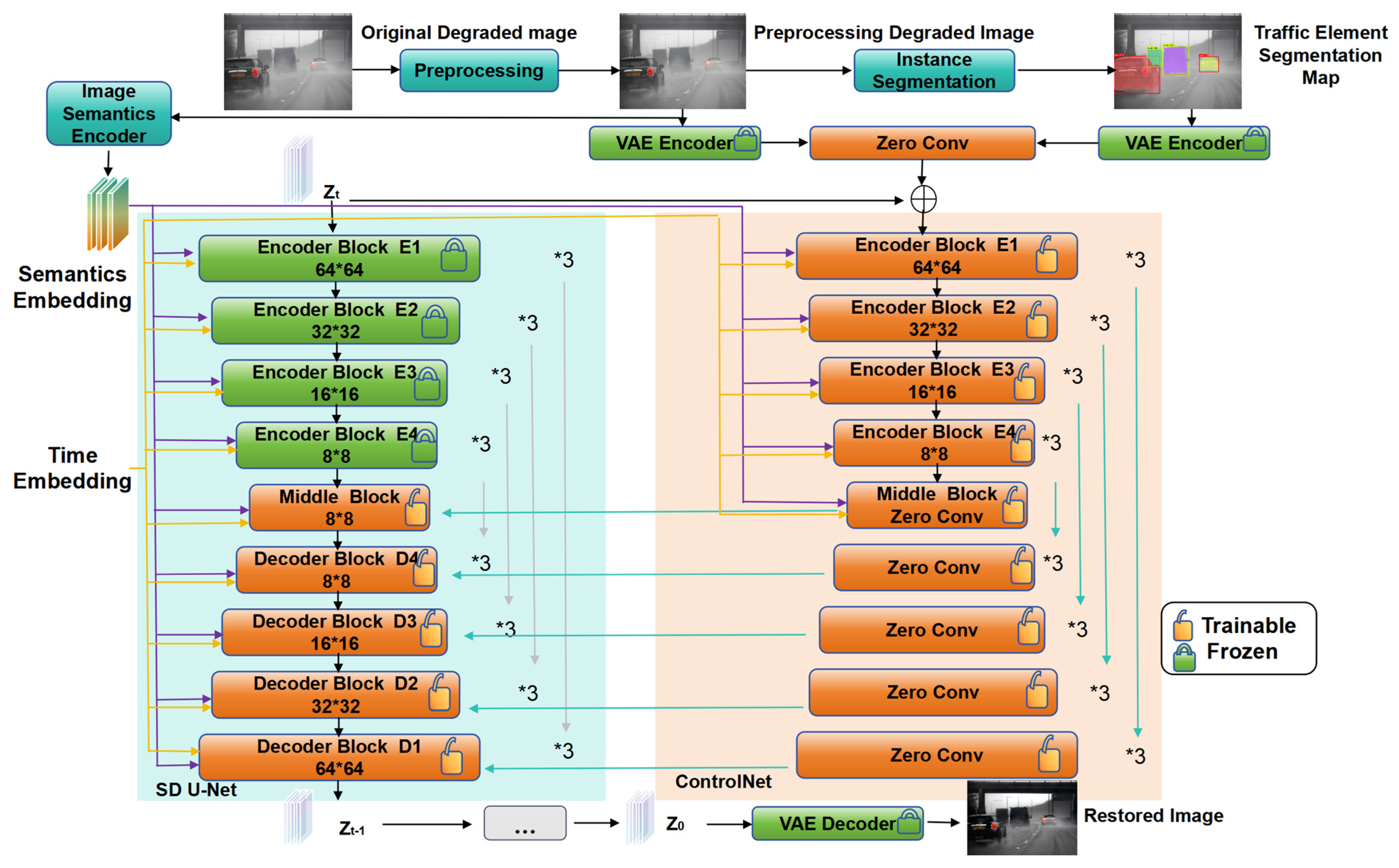
Network structure of traffic degradation image restoration model (TDIRM).
Figure 5.
Network structure of traffic degradation image restoration model (TDIRM).
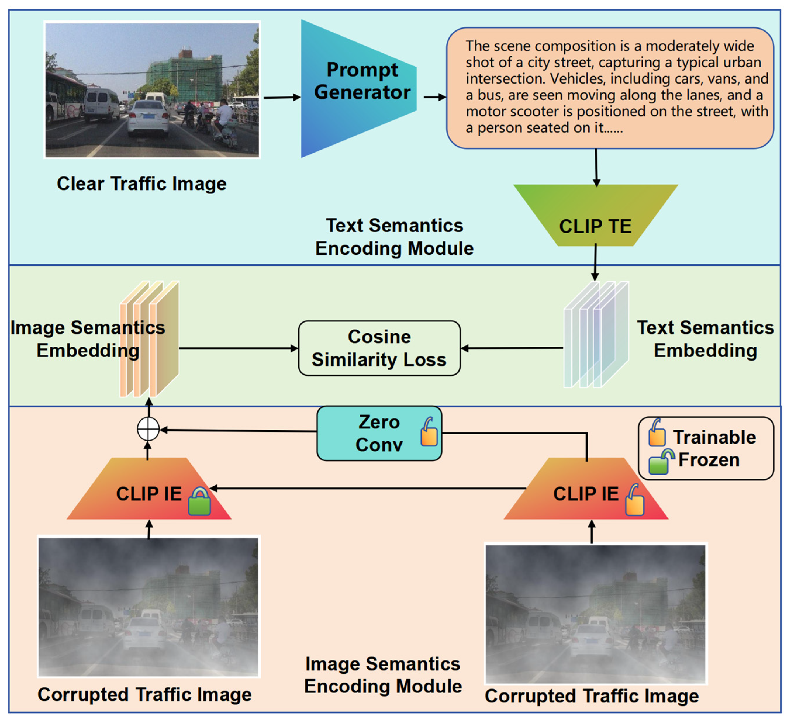
Figure 6.
Network structure of image semantics encoder module (ISE).
Figure 6.
Network structure of image semantics encoder module (ISE).
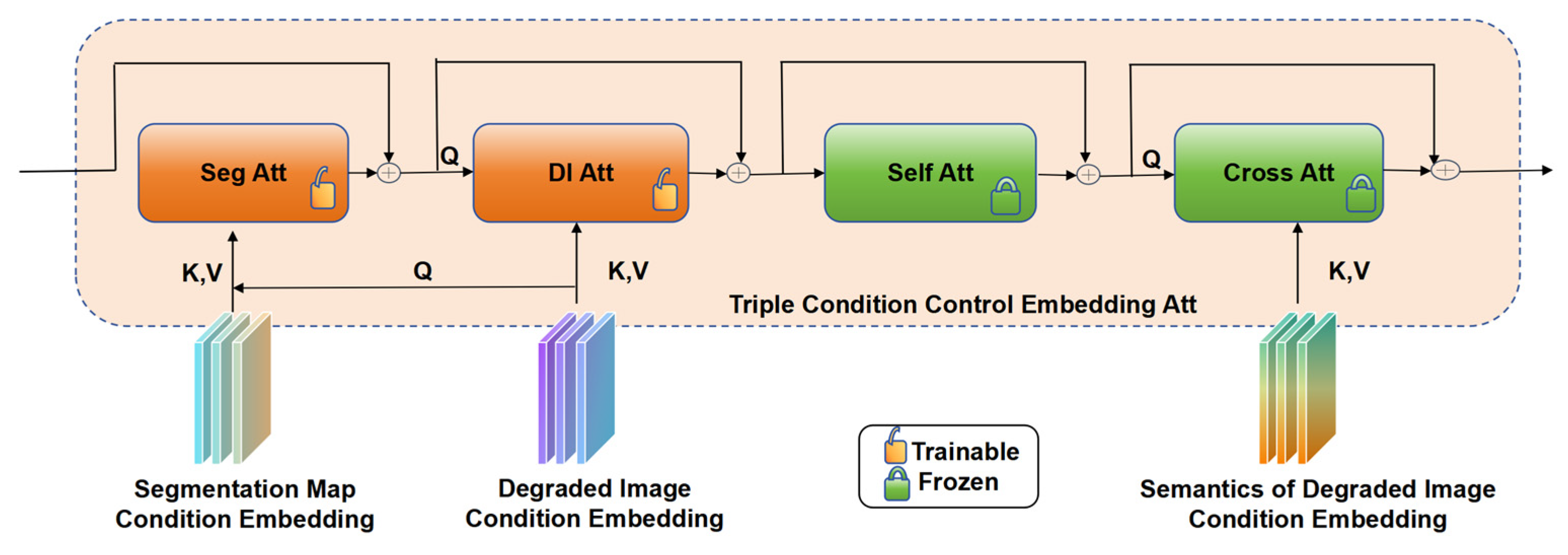
Figure 7.
Network structure of triple control embedding attention module (TCE).
Figure 7.
Network structure of triple control embedding attention module (TCE).
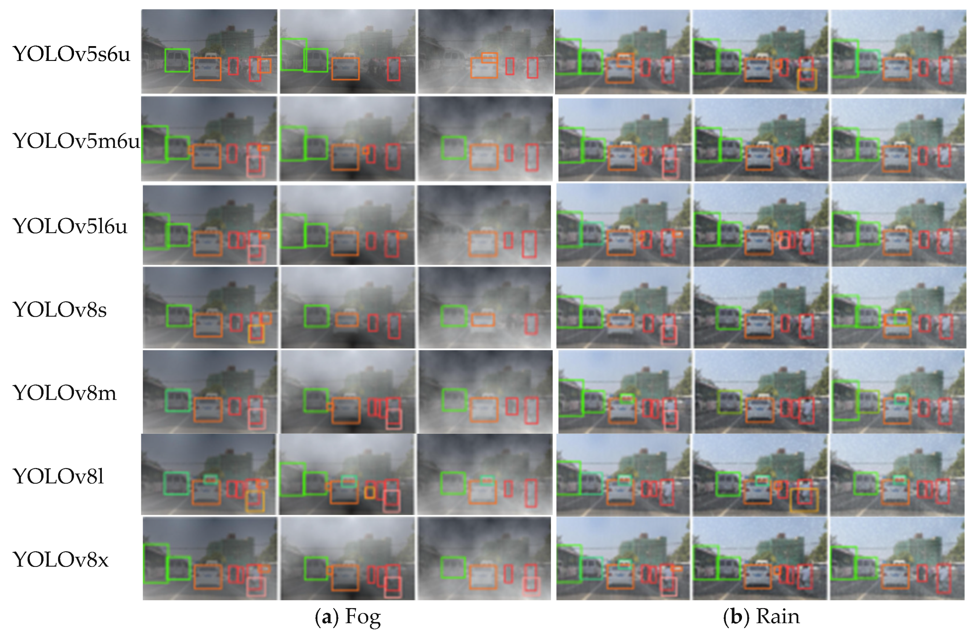
Figure 8.
Visualization results under fog and rain (three corruption levels).
Figure 8.
Visualization results under fog and rain (three corruption levels).
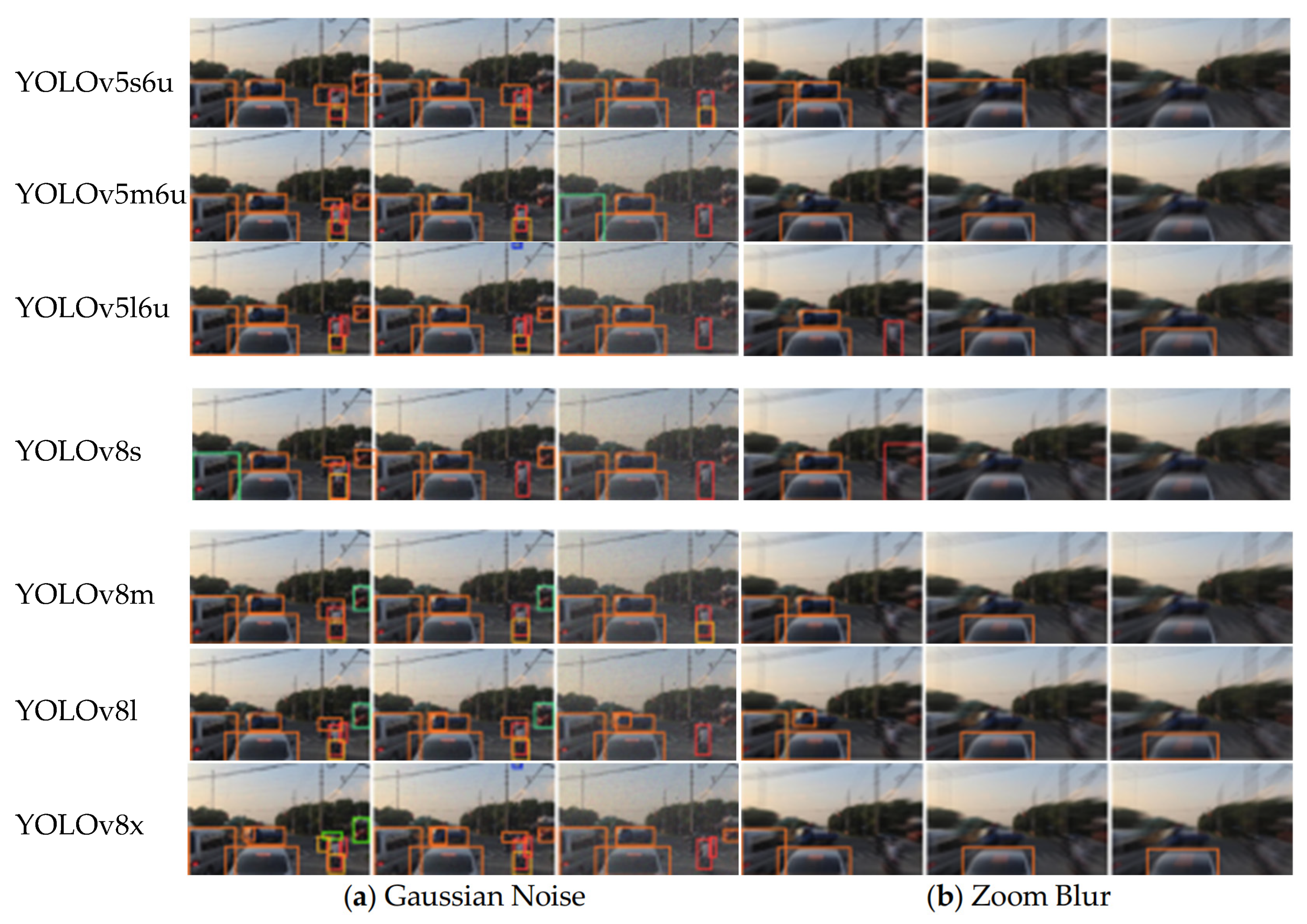
Figure 9.
Visualization results under Gaussian noise and zoom blur (three corruption levels).
Figure 9.
Visualization results under Gaussian noise and zoom blur (three corruption levels).
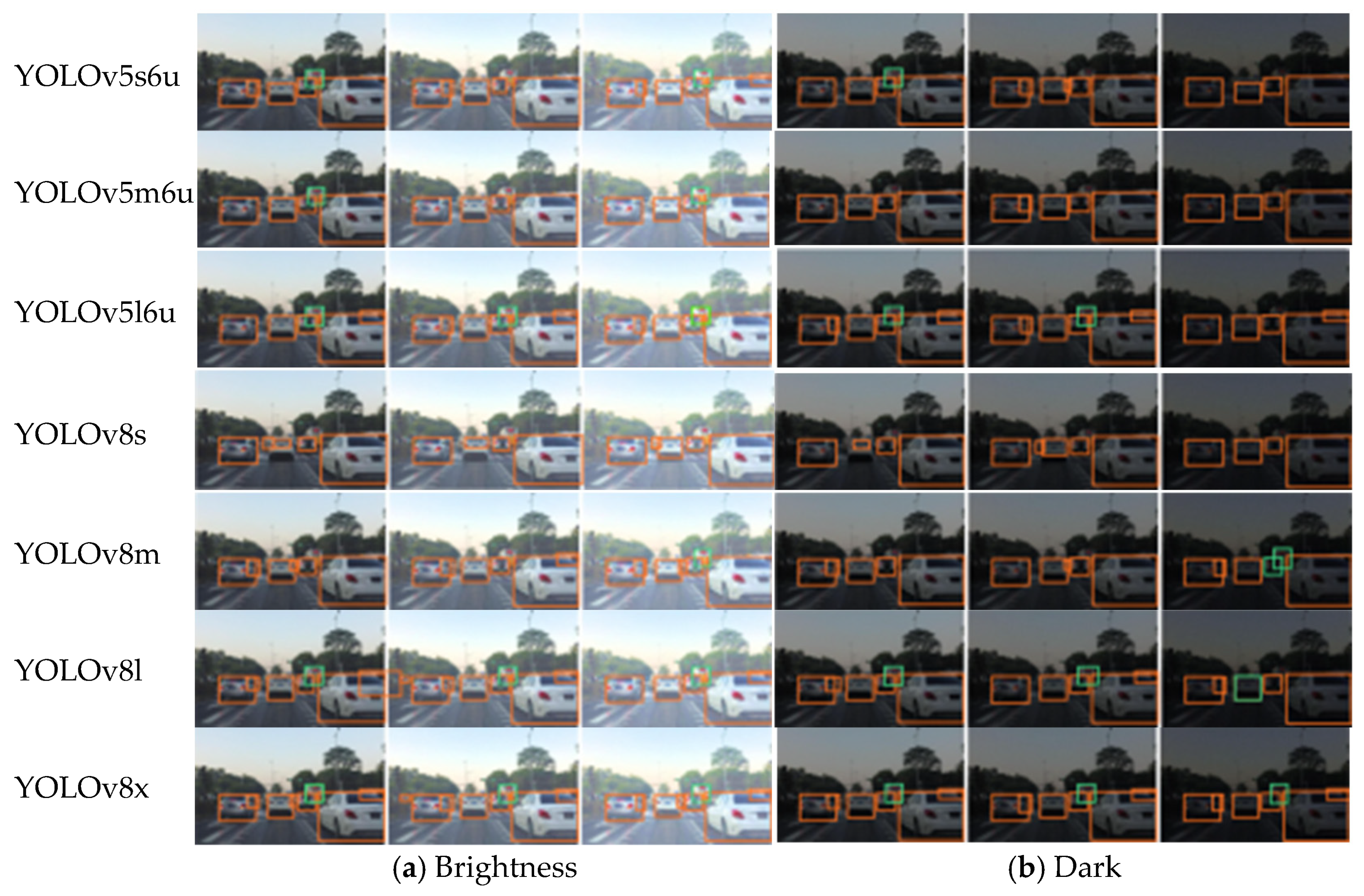
Figure 10.
Visualization results under brightness and dark (three corruption levels).
Figure 10.
Visualization results under brightness and dark (three corruption levels).
Figure 11.
Visualization results under occlusion and saturate (three corruption levels).
Figure 11.
Visualization results under occlusion and saturate (three corruption levels).
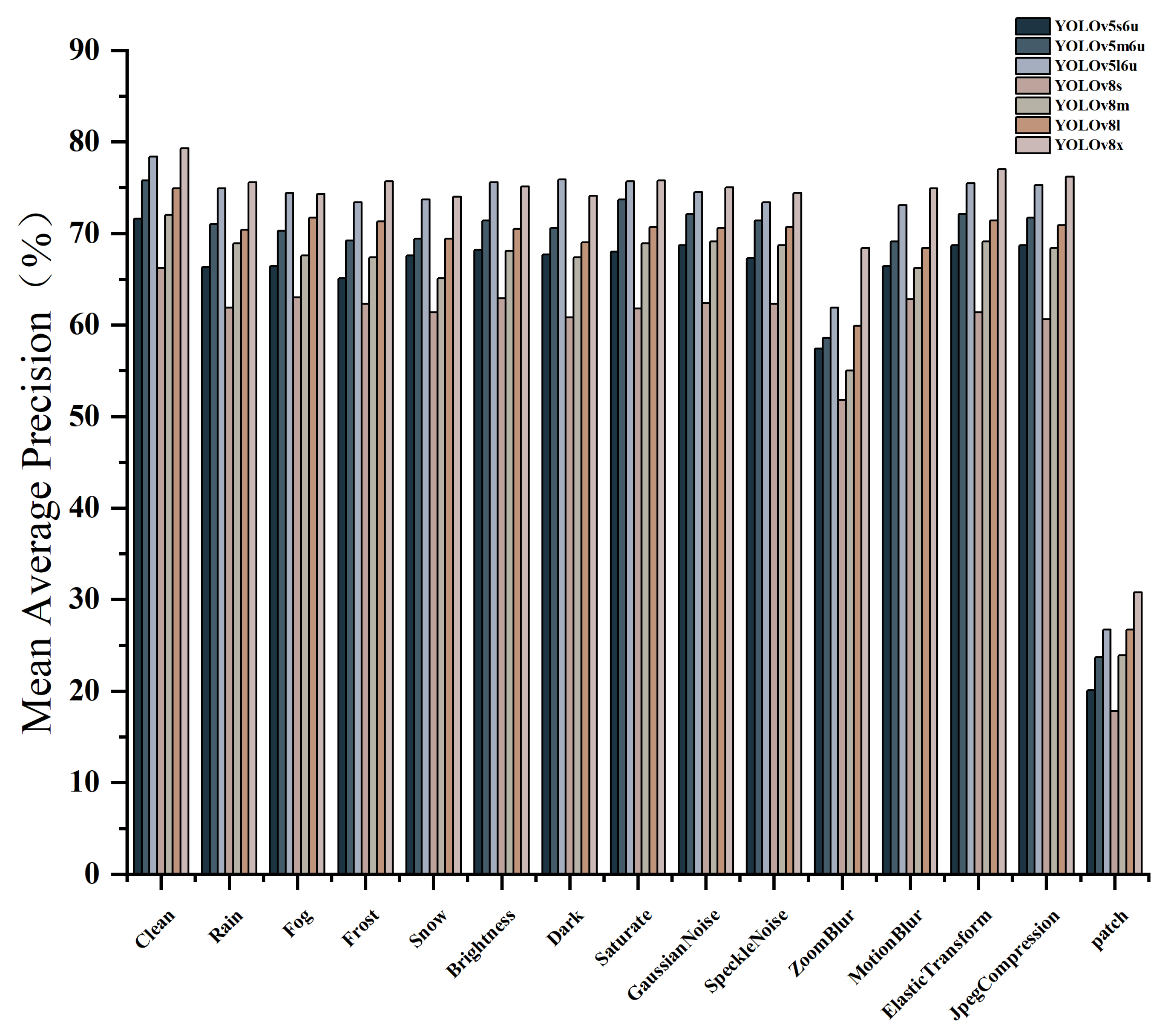
Figure 12.
Bar chart of benchmark results of YOLOv5 and YOLOv8. We show change in robustness metric (mAP50) under different corruption types at light level.
Figure 12.
Bar chart of benchmark results of YOLOv5 and YOLOv8. We show change in robustness metric (mAP50) under different corruption types at light level.
Figure 13.
Bar chart of benchmark results of YOLOv5 and YOLOv8. We show change in robustness metric (mAP50) under different corruption types at middle level.
Figure 13.
Bar chart of benchmark results of YOLOv5 and YOLOv8. We show change in robustness metric (mAP50) under different corruption types at middle level.
Figure 14.
Bar chart of benchmark results of YOLOv5 and YOLOv8. We show change in robustness metric (mAP50) under different corruption types at severe level.
Figure 14.
Bar chart of benchmark results of YOLOv5 and YOLOv8. We show change in robustness metric (mAP50) under different corruption types at severe level.
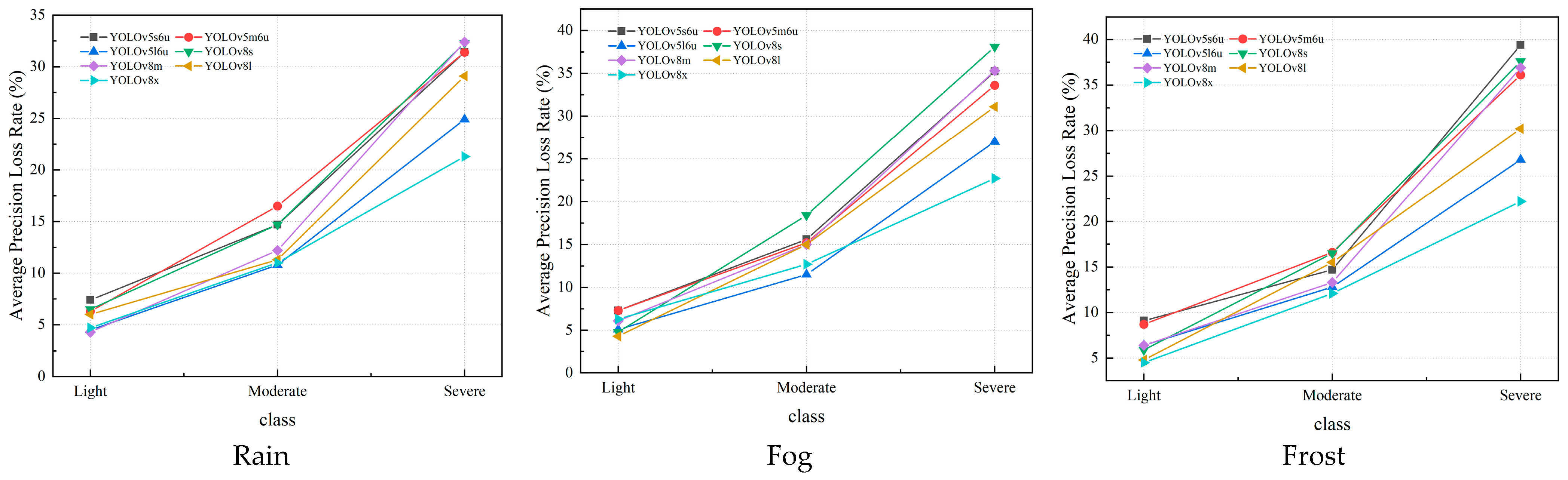
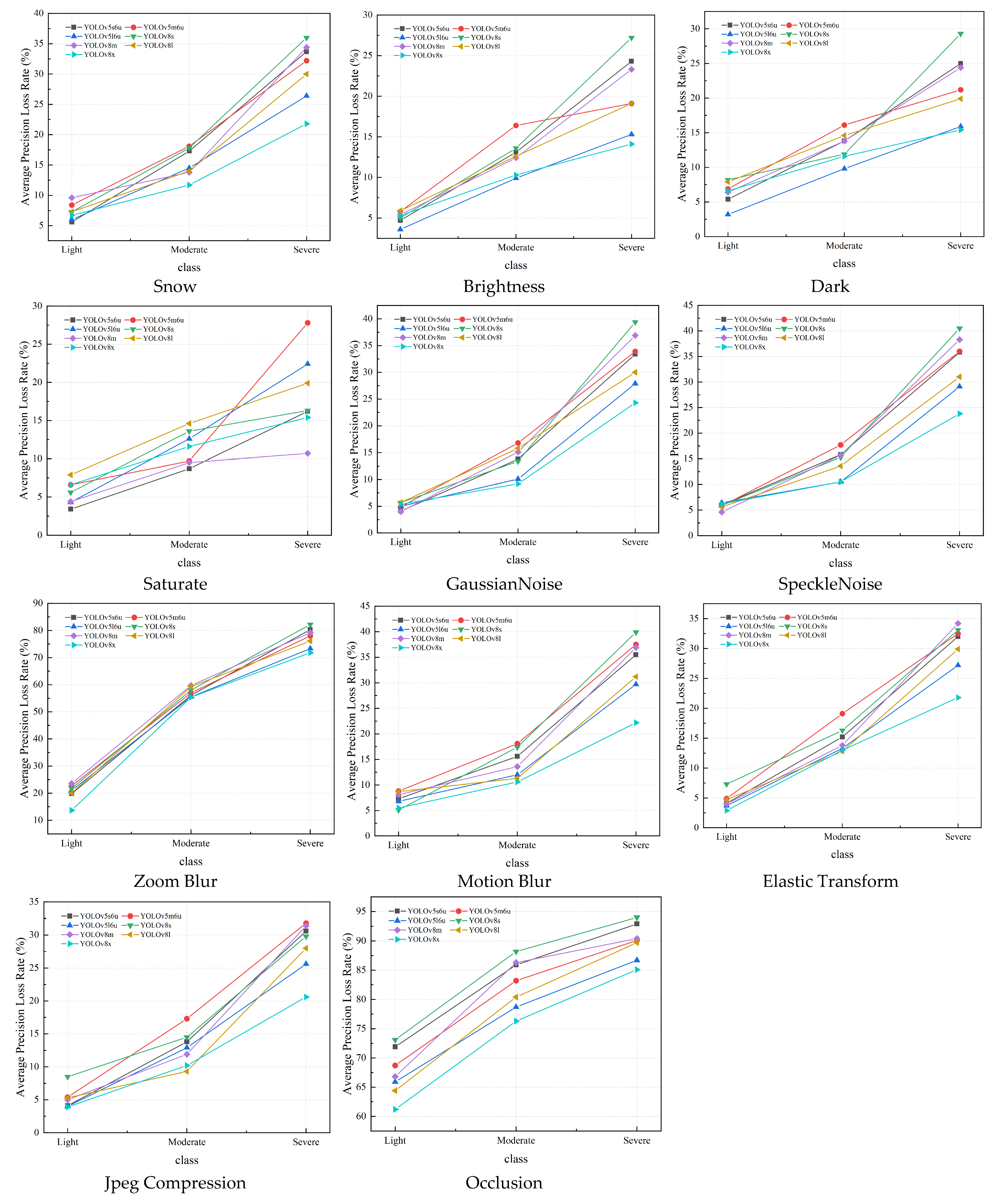
Figure 15.
The average precision loss rate of YOLOv5 and YOLOv8. The results are evaluated based on the car, truck, and bus classes (three corruption levels).
Figure 15.
The average precision loss rate of YOLOv5 and YOLOv8. The results are evaluated based on the car, truck, and bus classes (three corruption levels).
Figure 16.
Visualization results under fog and rain corruption under real conditions.
Figure 16.
Visualization results under fog and rain corruption under real conditions.
Figure 17.
Visualization results under snow and sand corruption under real conditions.
Figure 17.
Visualization results under snow and sand corruption under real conditions.
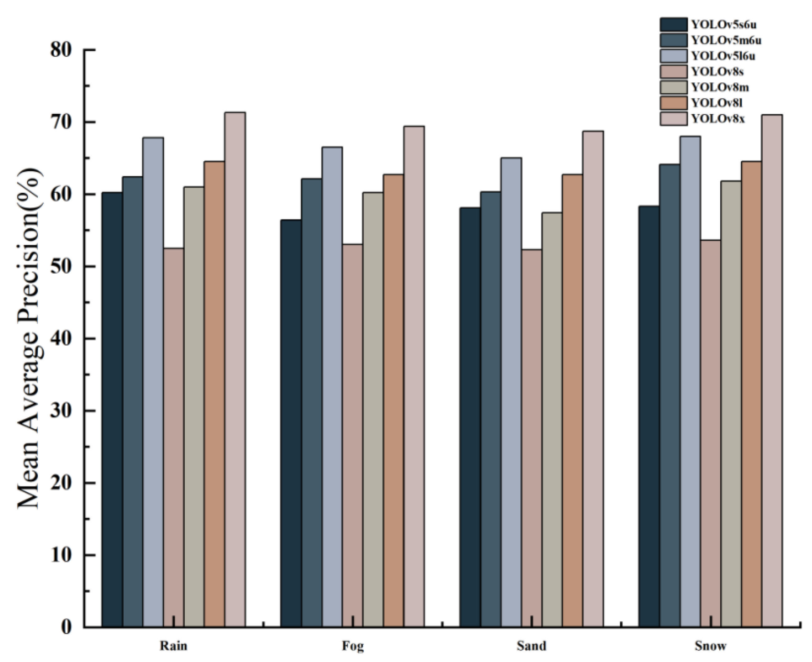
Figure 18.
Bar chart of benchmark results of YOLOv5 and YOLOv8 on real adverse weather dataset. We show change in robustness metric (mAP50).
Figure 18.
Bar chart of benchmark results of YOLOv5 and YOLOv8 on real adverse weather dataset. We show change in robustness metric (mAP50).
Figure 19.
Class activation mapping of cars. Each type of corruption is divided into three levels.
Figure 19.
Class activation mapping of cars. Each type of corruption is divided into three levels.
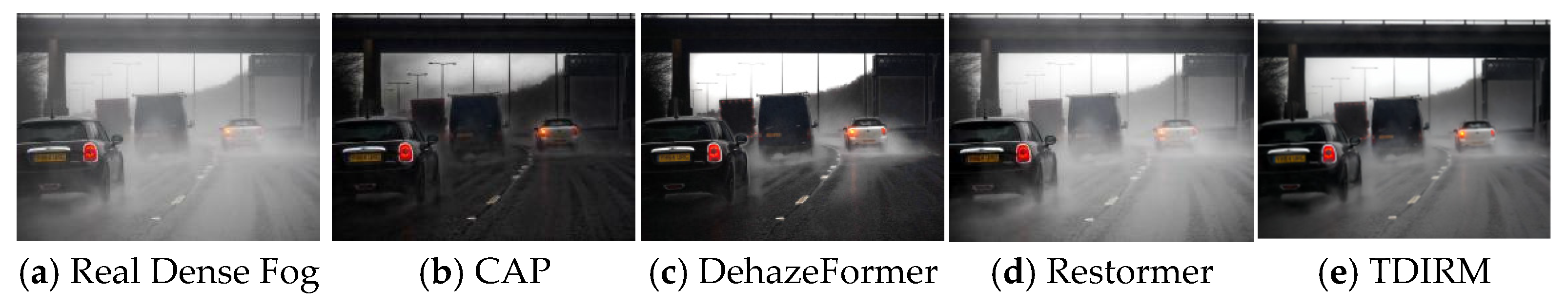
Figure 20.
Restoration effects comparison of real traffic dense fog images under different models.
Figure 20.
Restoration effects comparison of real traffic dense fog images under different models.
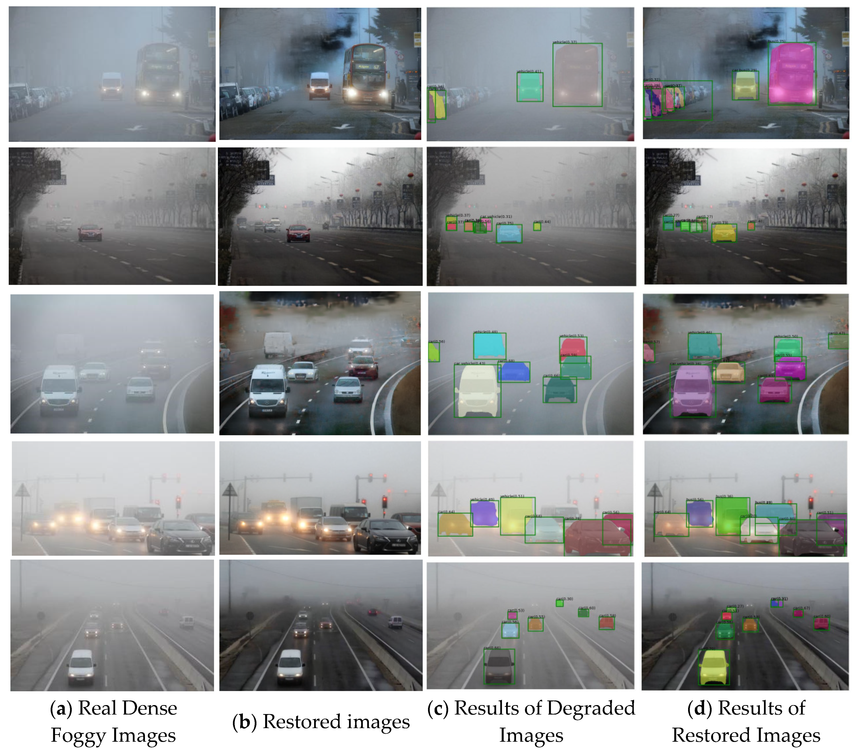
Figure 21.
Qualitative comparison of vehicle detection results before and after recovery in real traffic dense fog images.
Figure 21.
Qualitative comparison of vehicle detection results before and after recovery in real traffic dense fog images.
Table 1.
The methods for synthesizing corruption images.
Table 1.
The methods for synthesizing corruption images.
| Corruption Type | Methods |
|---|
| Snow | Predefined severities {1, 3, 5}, add a {10%, 20%, 30%}-opacity gray mask layer, reduce its brightness by 20%. |
| Fog | Predefined severities {1, 3, 5}, add a {10%, 20%, 30%}-opacity gray mask layer, reduce the brightness by 20%. |
| Rain | Add raindrop (size = (0.025, 0.05), speed = (0.25, 0.05)), add splatter with predefined severities {1, 2, 3}, add motion blur (k = 3), reduce the brightness by 20%. |
| Frost | Predefined severities {1, 3, 5}, add a {10%, 20%, 30%}-opacity gray mask layer, reduce the brightness by 10%. |
| Brightness | Predefined severities {1, 3, 5}. |
| Dark | The brightness is multiplied by (0.7, 0.5, 0.3), add Gaussian Noise with (1–5, 5–10, 10–20), adjust hue and saturation with (−10–+10, −20–+20, −30–+30). |
| Saturate | Predefined severities {1, 3, 5}. |
| Gaussian noise | Predefined severities {1, 3, 5}. |
| Speckle noise | Predefined severities {1, 3, 5}. |
| Zoom blur | Predefined severities {1, 3, 5}. |
| Jpeg compression | Predefined severities {1, 3, 5}. |
| Motion blur | Predefined severities {1, 3, 5}. |
| Elastic transform | Predefined severities {1, 3, 5}. |
| Occlusion | Randomly delete (30%, 50%, 70%) of small areas in the image, with each area approximately covering (0.01–0.02%) of the total image area. |
Table 2.
Category of models used for testing.
Table 2.
Category of models used for testing.
| Category | Method | Anchor |
|---|
| One stage | YOLOv5 | Yes |
| | YOLOv8 | Yes |
| | SSD [4] | Yes |
| | CenterNet [6] | No |
| Two stage | Faster R-CNN [1] | Yes |
| | Mask R-CNN [17] | Yes |
| | RetinaNet [49] | Yes |
Table 3.
Details of the YOLOv5 and YOLOv8 models used for testing.
Table 3.
Details of the YOLOv5 and YOLOv8 models used for testing.
| Model | Backbone | Type | Anchor | Params (M) | FLOPs (B) |
|---|
| YOLOv5s6u | YOLOv5CSPDarknet | one stage | Yes | 7.2 | 16.5 |
| YOLOv5m6u | YOLOv5CSPDarknet | one stage | Yes | 21.2 | 49.0 |
| YOLOv5l6u | YOLOv5CSPDarknet | one stage | Yes | 46.5 | 109.1 |
| YOLOv8s | YOLOv8CSPDarknet | one stage | Yes | 11.2 | 28.6 |
| YOLOv8m | YOLOv8CSPDarknet | one stage | Yes | 25.9 | 78.9 |
| YOLOv8l | YOLOv8CSPDarknet | one stage | Yes | 43.7 | 165.2 |
| YOLOv8x | YOLOv8CSPDarknet | one stage | Yes | 68.2 | 257.3 |
Table 4.
The benchmark results of YOLOv5 and YOLOv8. We show robustness metric (mAP50) under each corruption based on the car, truck, and bus classes at light level.
Table 4.
The benchmark results of YOLOv5 and YOLOv8. We show robustness metric (mAP50) under each corruption based on the car, truck, and bus classes at light level.
| Type (mAP50) (%) | YOLOv5s6u | YOLOv5m6u | YOLOv5l6u | YOLOv8s | YOLOv8m | YOLOv8l | YOLOv8x |
| | Clean | 71.6 | 75.8 | 78.4 | 66.2 | 72.0 | 74.9 | 79.3 |
| Weather | Rain | 66.3 | 71.0 | 74.9 | 61.9 | 68.9 | 70.4 | 75.6 |
| Fog | 66.4 | 70.3 | 74.4 | 63.0 | 67.6 | 71.7 | 74.3 |
| Frost | 65.1 | 69.2 | 73.4 | 62.3 | 67.4 | 71.3 | 75.7 |
| Snow | 67.6 | 69.4 | 73.7 | 61.4 | 65.1 | 69.4 | 74.0 |
| Color | Brightness | 68.2 | 71.4 | 75.6 | 62.9 | 68.1 | 70.5 | 75.1 |
| Dark | 67.7 | 70.6 | 75.9 | 60.8 | 67.4 | 69.0 | 74.1 |
| Saturate | 68.0 | 73.7 | 75.7 | 61.8 | 68.9 | 70.7 | 75.8 |
| Noise and Blur | GaussianNoise | 68.7 | 72.1 | 74.5 | 62.4 | 69.1 | 70.6 | 75.0 |
| SpeckleNoise | 67.3 | 71.4 | 73.4 | 62.3 | 68.7 | 70.7 | 74.4 |
| ZoomBlur | 57.4 | 58.6 | 61.9 | 51.8 | 55.0 | 59.9 | 68.4 |
| MotionBlur | 66.4 | 69.1 | 73.1 | 62.8 | 66.2 | 68.4 | 74.9 |
| Transform | ElasticTransform | 68.7 | 72.1 | 75.5 | 61.4 | 69.1 | 71.4 | 77.0 |
| JpegCompression | 68.7 | 71.7 | 75.3 | 60.6 | 68.4 | 70.9 | 76.2 |
| Occlusion | 20.1 | 23.7 | 26.7 | 17.8 | 23.9 | 26.7 | 30.8 |
Table 5.
The benchmark results of YOLOv5 and YOLOv8. We show robustness metric (mAP50) under each corruption based on the car, truck, and bus classes at middle level.
Table 5.
The benchmark results of YOLOv5 and YOLOv8. We show robustness metric (mAP50) under each corruption based on the car, truck, and bus classes at middle level.
| Type (mAP50) (%) | YOLOv5s6u | YOLOv5m6u | YOLOv5l6u | YOLOv8s | YOLOv8m | YOLOv8l | YOLOv8x |
| | Clean | 71.6 | 75.8 | 78.4 | 66.2 | 72.0 | 74.9 | 79.3 |
| Weather | Rain | 61.1 | 63.3 | 69.9 | 56.5 | 63.2 | 66.4 | 70.6 |
| Fog | 60.4 | 64.3 | 69.4 | 54.0 | 61.2 | 63.7 | 69.2 |
| Frost | 61.1 | 63.2 | 68.4 | 55.3 | 62.4 | 63.3 | 69.7 |
| Snow | 59.2 | 62.1 | 67.0 | 54.4 | 62.1 | 64.4 | 70.0 |
| Color | Brightness | 62.2 | 63.4 | 70.6 | 57.2 | 63.1 | 65.5 | 71.1 |
| Dark | 61.7 | 63.6 | 70.7 | 58.3 | 62.1 | 64.0 | 70.1 |
| Saturate | 61.0 | 62.7 | 71.6 | 59.8 | 62.9 | 64.7 | 71.8 |
| Noise and Blur | GaussianNoise | 61.7 | 63.1 | 70.5 | 57.3 | 61.1 | 63.1 | 72.0 |
| SpeckleNoise | 60.3 | 62.4 | 70.2 | 56.1 | 60.7 | 64.7 | 71.0 |
| ZoomBlur | 31.4 | 32.6 | 34.9 | 27.8 | 29.0 | 30.5 | 35.4 |
| MotionBlur | 60.4 | 62.1 | 69.0 | 54.7 | 62.2 | 66.4 | 70.9 |
| Transform | ElasticTransform | 60.7 | 61.3 | 68.0 | 55.4 | 62.1 | 65.3 | 69.0 |
| JpegCompression | 61.7 | 62.7 | 68.3 | 56.6 | 63.4 | 67.9 | 71.2 |
| Occlusion | 10.1 | 12.7 | 16.7 | 7.8 | 9.9 | 14.7 | 18.8 |
Table 6.
The benchmark results of YOLOv5 and YOLOv8. We show robustness metric (mAP50) under each corruption based on the car, truck, and bus classes at severe level.
Table 6.
The benchmark results of YOLOv5 and YOLOv8. We show robustness metric (mAP50) under each corruption based on the car, truck, and bus classes at severe level.
| Type (mAP50) (%) | YOLOv5s6u | YOLOv5m6u | YOLOv5l6u | YOLOv8s | YOLOv8m | YOLOv8l | YOLOv8x |
| | Clean | 71.6 | 75.8 | 78.4 | 66.2 | 72.0 | 74.9 | 79.3 |
| Weather | Rain | 49.1 | 52.0 | 58.9 | 44.8 | 48.7 | 53.1 | 62.4 |
| Fog | 46.4 | 50.3 | 57.2 | 41.0 | 46.6 | 51.6 | 61.3 |
| Frost | 43.4 | 48.4 | 57.4 | 41.3 | 45.4 | 52.3 | 61.7 |
| Snow | 47.5 | 51.4 | 57.7 | 42.4 | 47.2 | 52.4 | 62.0 |
| Color | Brightness | 54.2 | 61.3 | 66.4 | 48.2 | 55.2 | 60.6 | 68.1 |
| Dark | 53.7 | 59.7 | 65.9 | 46.8 | 54.4 | 60.0 | 67.1 |
| Saturate | 55.1 | 60.7 | 65.7 | 47.8 | 55.9 | 62.7 | 70.8 |
| Noise and Blur | GaussianNoise | 47.7 | 50.1 | 56.5 | 40.1 | 45.4 | 52.4 | 60.0 |
| SpeckleNoise | 46.0 | 48.5 | 55.6 | 39.4 | 44.4 | 51.7 | 60.4 |
| ZoomBlur | 14.1 | 16.7 | 20.9 | 11.8 | 15.0 | 17.9 | 22.4 |
| MotionBlur | 46.2 | 47.4 | 55.1 | 39.8 | 45.4 | 51.5 | 61.7 |
| Transform | ElasticTransform | 48.7 | 51.2 | 57.1 | 44.3 | 47.4 | 52.5 | 62.0 |
| JpegCompression | 49.7 | 51.7 | 58.3 | 46.5 | 49.4 | 53.9 | 63.0 |
| Occlusion | 5.1 | 7.5 | 10.4 | 4.0 | 6.9 | 7.7 | 11.8 |
Table 7.
The benchmark results of YOLOv5 and YOLOv8 on real adverse weather dataset.
Table 7.
The benchmark results of YOLOv5 and YOLOv8 on real adverse weather dataset.
| Type (mAP50) (%) | YOLOv5s6u | YOLOv5m6u | YOLOv5l6u | YOLOv8s | YOLOv8m | YOLOv8l | YOLOv8x |
| Rain | 60.2 | 62.4 | 67.8 | 52.5 | 61.0 | 64.5 | 71.3 |
| Fog | 56.4 | 62.1 | 66.5 | 53.0 | 60.2 | 62.7 | 69.4 |
| Sandstorm | 58.1 | 60.3 | 65.0 | 52.3 | 57.4 | 62.7 | 68.7 |
| Snow | 58.3 | 64.1 | 68.0 | 53.6 | 61.8 | 64.5 | 71.0 |
Table 8.
The benchmark results of remaining models. We show robustness metric (mAP50) under each corruption based on the car, truck, and bus classes at light level.
Table 8.
The benchmark results of remaining models. We show robustness metric (mAP50) under each corruption based on the car, truck, and bus classes at light level.
| Type (mAP50) (%) | SSD | CenterNet | Faster R-CNN | Mask R-CNN | RetinaNet |
| | Clean | 72.0 | 67.1 | 79.7 | 80.6 | 78.6 |
| Weather | Rain | 67.2 | 63.2 | 75.8 | 75.9 | 74.4 |
| Fog | 66.1 | 63.0 | 74.7 | 74.4 | 76.1 |
| Frost | 66.5 | 64.2 | 76.0 | 76.6 | 74.2 |
| Snow | 65.8 | 64.3 | 75.5 | 77.3 | 75.4 |
| Color | Brightness | 70.3 | 66.7 | 79.0 | 78.4 | 75.1 |
| Dark | 68.4 | 62.5 | 74.6 | 73.4 | 73.7 |
Saturate
| 69.0 | 64.9 | 76.8 | 76.6 | 75.7 |
| Noise and Blur | GaussianNoise | 68.3 | 65.2 | 76.4 | 76.3 | 75.6 |
| SpeckleNoise | 67.9 | 65.1 | 75.7 | 76.0 | 74.6 |
| ZoomBlur | 56.0 | 53.3 | 67.1 | 68.2 | 65.1 |
| MotionBlur | 65.4 | 62.3 | 73.2 | 73.7 | 72.9 |
| Transform | ElasticTransform | 68.3 | 63.2 | 75.7 | 75.9 | 74.2 |
| JpegCompression | 67.9 | 64.0 | 76.4 | 76.8 | 75.9 |
| Occlusion | 21.3 | 20.4 | 33.4 | 35.7 | 30.6 |
Table 9.
The benchmark results of remaining models. We show robustness metric (mAP50) under each corruption based on the car, truck, and bus classes at middle level.
Table 9.
The benchmark results of remaining models. We show robustness metric (mAP50) under each corruption based on the car, truck, and bus classes at middle level.
| Type (mAP50) (%) | SSD | CenterNet | Faster R-CNN | Mask R-CNN | RetinaNet |
| | Clean | 72.0 | 67.1 | 79.7 | 80.6 | 78.6 |
| Weather | Rain | 62.4 | 58.6 | 71.4 | 72.6 | 69.0 |
| Fog | 61.2 | 59.1 | 70.7 | 70.9 | 68.9 |
| Frost | 62.0 | 55.5 | 70.7 | 71.8 | 67.4 |
| Snow | 60.6 | 57.0 | 69.2 | 70.4 | 67.8 |
| Color | Brightness | 62.7 | 58.3 | 70.4 | 72.0 | 70.1 |
| Dark | 59.3 | 55.1 | 69.4 | 71.5 | 68.7 |
| Saturate | 63.0 | 58.6 | 70.6 | 74.4 | 71.4 |
| Noise and Blur | GaussianNoise | 61.6 | 57.0 | 69.4 | 71.4 | 70.0 |
| SpeckleNoise | 61.0 | 58.4 | 67.1 | 70.6 | 69.8 |
| ZoomBlur | 33.7 | 28.9 | 35.7 | 38.8 | 36.4 |
| MotionBlur | 59.9 | 56.4 | 67.5 | 69.5 | 68.4 |
| Transform | ElasticTransform | 60.7 | 57.8 | 67.0 | 70.5 | 69.2 |
| JpegCompression | 61.6 | 57.5 | 68.4 | 71.4 | 70.6 |
| Occlusion | 11.5 | 9.6 | 18.5 | 21.4 | 18.4 |
Table 10.
The benchmark results of remaining models. We show robustness metric (mAP50) under each corruption based on the car, truck, and bus classes at severe level.
Table 10.
The benchmark results of remaining models. We show robustness metric (mAP50) under each corruption based on the car, truck, and bus classes at severe level.
| Type (mAP50) (%) | SSD | CenterNet | Faster R-CNN | Mask R-CNN | RetinaNet |
| | Clean | 72.0 | 67.1 | 79.7 | 80.6 | 78.6 |
| Weather | Rain | 50.5 | 46.6 | 59.9 | 61.7 | 57.4 |
| Fog | 47.3 | 44.1 | 54.5 | 60.2 | 57.0 |
| Frost | 48.5 | 45.3 | 56.4 | 59.7 | 56.8 |
| Snow | 49.0 | 46.9 | 56.9 | 60.4 | 55.3 |
| Color | Brightness | 53.8 | 52.7 | 64.2 | 66.5 | 63.1 |
| Dark | 50.1 | 49.4 | 60.4 | 62.7 | 61.4 |
| Saturate | 54.0 | 53.2 | 65.2 | 67.4 | 63.0 |
| Noise and Blur | GaussianNoise | 48.1 | 45.9 | 56.0 | 58.7 | 56.1 |
| SpeckleNoise | 46.2 | 44.8 | 54.8 | 58.5 | 55.4 |
| ZoomBlur | 14.5 | 12.7 | 20.4 | 23.8 | 20.0 |
| MotionBlur | 46.0 | 43.7 | 54.4 | 57.1 | 53.4 |
| Transform | ElasticTransform | 47.1 | 43.5 | 55.1 | 57.6 | 55.9 |
| JpegCompression | 49.4 | 44.5 | 54.9 | 59.1 | 56.1 |
| Occlusion | 5.9 | 5.0 | 9.5 | 12.7 | 10.1 |
Table 11.
Quantitative comparison of different dehaze models on paired synthesized traffic foggy images.
Table 11.
Quantitative comparison of different dehaze models on paired synthesized traffic foggy images.
| Method | PSNR | SSIM | NIQE |
|---|
| DCP | 21.95 | 0.924 | 4.927 |
| CAP | 23.36 | 0.931 | 4.815 |
| FFA-Net | 29.71 | 0.955 | 4.196 |
| AOD-Net | 22.47 | 0.893 | 4.335 |
| DehazeFormer | 30.57 | 0.976 | 3.973 |
| Restormer | 29.54 | 0.973 | 4.415 |
| DiffBIR | 28.49 | 0.958 | 4.229 |
| WeatherDiff | 26.72 | 0.952 | 4.341 |
Table 12.
Quantitative comparison of vehicle detection results before and after recovery in real traffic dense fog images.
Table 12.
Quantitative comparison of vehicle detection results before and after recovery in real traffic dense fog images.
| Image Type | mAP50 (%) | Recall (%) | Precision (%) |
|---|
| Real traffic foggy images | 78.62 | 75.60 | 87.15 |
| The restored images | 85.54 | 83.18 | 92.26 |
Table 13.
Ablation experiments for different modules of TDIRM.
Table 13.
Ablation experiments for different modules of TDIRM.
| Module | PSNR | SSIM | NIQE |
|---|
| CLIP IE + SelfAtt | 23.54 | 0.851 | 4.928 |
| ISE + SelfAtt | 26.39 | 0.917 | 4.472 |
| CLIP IE + TCEAtt | 27.42 | 0.936 | 4.324 |
| ISE + TCEAtt (TDIRM) | 30.69 | 0.968 | 3.880 |
Table 14.
Ablation experiments for different control embedding of TDIRM.
Table 14.
Ablation experiments for different control embedding of TDIRM.
| Control Embedding | PSNR | SSIM | NIQE |
|---|
| DIE | 25.93 | 0.891 | 4.453 |
| SE + DIE | 28.71 | 0.944 | 4.126 |
| DIE + SegE | 29.72 | 0.953 | 4.045 |
| SE + SegE | 27.64 | 0.925 | 4.237 |
| SE + DIE + SegE (TDIRM) | 30.69 | 0.968 | 3.880 |


