Research on the Single-Leg Compliance Control Strategy of the Hexapod Robot for Collapsible Terrains

Abstract

Legged robots often encounter the problem that the foot-end steps into empty spaces due to terrain collapse in complex environments such as mine tunnels and coal shafts, which in turn causes body instability. Aiming at this problem, this paper takes the hexapod robot as the research object and proposes a multi-segmented electrically driven single-leg compliance control strategy for robots with tripod and quadrupedal gaits, to reduce the impact when the foot-end touches the ground, and thus to improve the stability of the robot. First, this paper analyzes the kinematic and dynamic models of the multi-segmented electrically driven single leg of the hexapod robot. Then, the minimum tipping angle of the fuselage is obtained based on force-angle stability margin (FASM) and used as the index to design the single-leg pit-probing control algorithm based on position impedance control and the single-leg touchdown force adjustment control algorithm based on inverse dynamics control. Finally, this paper designs a finite state machine to switch between different control strategies of the multi-segmented electrically driven single leg of the hexapod robot, and the vertical dynamic impact characteristic index is applied to evaluate the effect of single-leg impedance control. The simulation and prototype test results show that the proposed method significantly reduces the foot-end touchdown force and improves the walking stability of the hexapod robot in complex environments compared with the multi-segmented electrically driven single leg without the compliance control strategy.

1. Introduction

In recent years, legged robots have become a research hotspot in robotics due to their excellent terrain adaptability [1,2]. Among the existing legged robots, the hexapod robots have higher walking stability and anti-tipping ability compared with quadruped and biped robots [3]. Therefore, they have received increasingly extensive attention in fields such as disaster relief [4]. Among the existing motion control methods for hexapod robots, control based on dynamic models can significantly improve the motion performance of hexapod robots [5]. The walking stability of legged robots is deeply affected by the impact between the foot-end and the ground when they perform tasks in different terrains. In current academic research, reducing the impact of the foot-end touching the ground through compliant control is an important research direction [6].

Compliant control can be further divided into passive and active compliant control [7]. Passive compliant control relies on mechanical structural components. Hutter et al. added series elastic actuators (SEAs) to the robot leg to improve motion compliance [8]. However, its compliance is limited by the material selection, processing, and stiffness and deformation range of the elastomer. Active compliance control adjusts the force–position relationship of the robot in real time through sensor feedback and control algorithms to adapt to the external environment. Hogan proposed two classic impedance control methods [9,10], the force-based and position-based impedance methods (also known as admittance control). Both methods establish a relationship between the end-effector position and the touchdown force of the robot and indirectly control the contact force with the environment by using the change in the end-effector pose. The team of Thiago Boaventura from the Italian Institute of Technology (IIT) researched force-based impedance control for hydraulic legs [11]. By modeling and analyzing the valve control system and combining force loop compensation, they improved the response speed of force-based impedance control, but it has not been verified on electrically driven robots. The team of Felix proposed a new controller that integrates feed-forward contact force and impedance control for the robot and verified its excellent impedance adjustment ability in high dynamic motion through experiments [12]. Wang et al. achieved a good force-tracking response based on admittance control in a known environment, with the steady-state error being almost zero and a fast response speed [13].

In post-disaster rescue operations, hexapod robots often encounter local ground collapses or slippage when their feet contact the terrain [14], which can lead to a loss of stability during locomotion. Therefore, when unexpected events such as foot misplacement occur under different gaits, it is essential to first assess the robot’s stability. A state ma-chine should then be employed to adjust the control strategy in real time based on the status flags, thereby enhancing overall stability. Since hexapod robots exhibit distinct dynamic characteristics under different gaits [15], the impact of foot misplacement on overall stability also varies with the gait type. At present, the mainstream methods for real-time stability monitoring include the zero moment point (ZMP) method, the force-angle stability margin (FASM), and the moment-height stability (MHS) method. ZMP is defined as the minimum distance from the equivalent zero-moment point—where the moments in the x and y directions are zero on the horizontal plane to the edge of the support polygon, and this distance is used as the stability margin at the current moment. Zhang et al. [16] applied the FASM method, which evaluates dynamic stability based on the relationship between the resultant force and the support polygon. FASM has become one of the dominant approaches for stability assessment in legged robots. Building on FASM, Moosavian and Alipour proposed the MHS (moment-height stability) method [17], which is primarily used for assessing the stability of robots such as aerial manipulators. MHS is defined as the minimum value of the product of the unit vector along the support polygon edge, the equivalent moment acting on that edge, and the robot’s moment of inertia relative to the same edge. Roan, Philip R., and others conducted a comparative analysis of ZMP, FASM, and MHS, and performed tipping experiments on robots. The results demonstrated that FASM and MHS are more effective than ZMP in dynamic stability evaluation. Among them, FASM showed higher sensitivity and a certain degree of predictive capability compared to MHS. Therefore, this paper adopts the force-angle stability margin (FASM) as the stability criterion, using the minimum tipping angle as the stability index. Corresponding state flags are output and integrated with a finite state machine for decision-making control.

The subsequent content is arranged as follows: Section 1 provides a review of existing control strategies for legged robots. Section 2 analyzes the leg structure of the legged robot and presents the kinematic and dynamic modeling. Section 3 sets the minimum tipping angle index for the entire robot based on the FASM method and makes decisions on tasks such as pit detection and ground force adjustment using a state machine. Section 4 proposes a position-based impedance control scheme, optimizes impedance control parameters, and conducts simulation analysis. Section 5 proposes a force-based impedance control scheme, performing stability and simulation analysis on the designed control. Section 6 presents prototype experiments based on the previous research, comparing and analyzing the results from simulations and experiments. Section 7 summarizes the work of the entire paper.

2. Single-Leg Kinematics and Dynamics Modelling

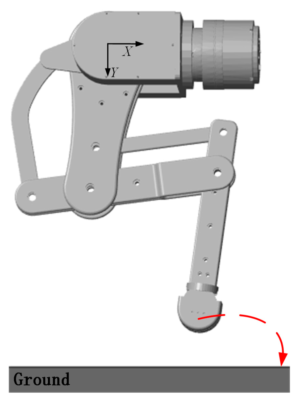
2.1. Single-Leg Structural Analysis

The single-leg design of the hexapod robot under study refers to the leg structures of mammals such as cheetahs [18], as shown in Figure 1. The hip and the thigh are directly driven by motor 1 and motor 2, respectively; the shank is indirectly driven by motor 3 through a parallelogram mechanism; and the ankle is a passive link, which is indirectly driven by the parallelogram mechanism composed of the thigh and the shank. The parallelogram mechanism moves up motor 3, which drives the shank, thereby reducing the inertia of a single leg.

2.2. Single-Leg Kinetic Modeling

The simplified diagram of the single-leg structure, including the centroid coordinate systems of each link and the joint coordinate systems, is shown in Figure 2, where ${\theta }_A$, ${\theta }_B$, and ${\theta }_C$ are the rotation angles of motor 1, 2, and 3, respectively.

According to the properties of the parallelogram mechanism, ${\theta }_B=-{\theta }_D={\theta }_E={\theta }_F={\theta }_G=-{\theta }_H=-{\theta }_I$. Define the length of the link between joint $i$ and joint $j$ as $l_{ij}$ (e.g., the length of the link between joint $A$ and joint $B$ is $l_{AB}$). Define the length of the centroid of each link relative to its own rotational joint coordinate system as $l_{C_i}$ (e.g., the coordinate of the centroid $C_1$ of the link between joint $A$ and joint $B$ relative to the coordinate system $\left\{A\right\}$ is ${(\begin{array}{ccc}0& 0& -l_{C_i}\end{array})}^{\mathrm{T}}$).

Define $A\to C\to G\to I\to P$ as the main kinematic chain of the single-leg mechanism. According to the graphical method, the position vector $(p_x,p_y,p_z)$ of the end point P (foot-end) of the main kinematic chain relative to the base coordinate system is as follows:

$$\left\{\begin{array}{l}{p}_x=\cos {\theta }_A\left[-l_{GI}\sin ({\theta }_B+{\theta }_C)+\cos {\theta }_B(l_{CG}+l_{IP})\right]\\ p_y=\sin {\theta }_A\left[-l_{GI}\sin ({\theta }_B+{\theta }_C)+\cos {\theta }_B(l_{CG}+l_{IP})\right]\\ p_z=-l_{GI}\cos ({\theta }_B+{\theta }_C)-\sin {\theta }_B(l_{CG}+l_{IP})\end{array}\right.$$

(1)

2.3. Single-Leg Dynamic Modeling

For a single link of the leg, its active force is related to the first- and second-order kinematic differential quantities of the centroid of the link relative to the base coordinate. Considering the existence of the parallelogram closed-loop chain structure in the leg, the product exponential formula is first used to solve the kinematics of the centroid of each link [19,20]:

$${}^{\mathbf{0}}\mathit{T}_{C_i}={\displaystyle \prod _j\exp ({\widehat{\mathit{\xi }}}_j,{\theta }_j)}{\mathit{T}}_{C_i}$$

(2)

where ${\mathit{T}}_{C_i}$, ${}^{\mathbf{0}}\mathit{T}_{C_i}$ is the initial pose matrix and the pose matrix after homogeneous transformation of the centroid coordinate system {C_i} relative to the base coordinate system {0}, respectively. For {C_i}, ${\mathit{T}}_{C_i}=\left[\begin{array}{cc}{\mathit{I}}_{3\times 3}& R_{C_i}\\ {\mathbf{0}}_{1\times 3}& 1\end{array}\right]$, $R_{C_i}$ is the position vector of the centroid C_i relative to {0}, $\exp ({\widehat{\mathit{\xi }}}_j,{\theta }_j)$ is the product exponential formula, and ${\widehat{\mathit{\xi }}}_j$, ${\theta }_j$ are the Lie algebra of the screw coordinates and the joint rotation angle joint j, respectively.

From the transformation relationships among the homogeneous transformation matrix, the Jacobian matrix, and the motion screw, the mapping relationships between the velocity $V_{C_i}$, acceleration ${\mathit{\epsilon }}_{C_i}$ of the centroid of each link, and the active variables ${\theta }_A$, ${\theta }_B$, and ${\theta }_C$ can be obtained as:

$$\left\{\begin{array}{ll}{\mathit{V}}_{C_i}& =\left[\begin{array}{c}{\mathit{\omega }}_{C_i}\\ {\mathit{v}}_{C_i}\end{array}\right]={\left[{}^{\mathbf{0}}\dot{\mathit{T}}_{C_i}{}^{\mathbf{0}}\mathit{T}_{C_i}^{-1}\right]}^{\vee }\\ & =\{{\mathit{\xi }}_A,\mathrm{Ad}\left[\exp \right({\widehat{\mathit{\xi }}}_A,{\theta }_A\left)\right]{\xi }_B,\dots ,{\displaystyle \prod _j\mathrm{Ad}\left[\exp \right({\widehat{\mathit{\xi }}}_j,{\theta }_j\left)\right]{\mathit{\xi }}_i}\}\cdot \mathit{\Lambda }\cdot {(\begin{array}{ccc}{\dot{\theta }}_A& {\dot{\theta }}_B& {\dot{\theta }}_C\end{array})}^{\mathrm{T}}\\ & ={\mathit{J}}_{C_i}\dot{\mathit{\theta }}\\ {\mathit{\epsilon }}_{C_i}& =\left[\begin{array}{c}{\mathit{\alpha }}_{C_i}\\ {\mathit{a}}_{C_i}\end{array}\right]={\mathit{J}}_{C_i}\ddot{\mathit{\theta }}+{\dot{\mathit{\theta }}}^{\mathrm{T}}{\mathit{H}}_{C_i}\dot{\mathit{\theta }}\end{array}\right.$$

(3)

where ${[•]}^{\vee }$ is the isomorphic mapping from the Lie algebra to the six-dimensional vector, and ${\left[\begin{array}{cc}{\left[\mathit{\omega }\right]}_{\times }& \mathit{v}\\ 0& 0\end{array}\right]}^{\vee }=\left[\begin{array}{c}\mathit{\omega }\\ \mathit{v}\end{array}\right]$, where ${\left[\mathit{\omega }\right]}_{\times }$ is the skew symmetric matrix form of the three-dimensional vector $\mathit{\omega }$, $\mathrm{Ad}\left[\exp \right({\widehat{\mathit{\xi }}}_i,{\theta }_i\left)\right]$ is the adjoint transformation matrix of the screw, and $\mathit{\Lambda }$ is the transformation matrix between the first order differentials of the joint rotation angles (e.g., ${\dot{\theta }}_D$, ${\dot{\theta }}_F$, ${\dot{\theta }}_G$, ${\dot{\theta }}_I$) and $\dot{\mathit{\theta }}$. ${\mathit{J}}_{C_i}$ is the Jacobian matrix of the centroid C_i, and ${\mathit{H}}_{C_i}$ is the Hessian matrix of the centroid C_i.

By taking differentials on both sides of Equation (1), the mappings of the velocity $V_P$ and acceleration ${\mathit{\epsilon }}_P$ of the foot-end P with respect to ${\theta }_A$, ${\theta }_B$, ${\theta }_C$ can be obtained:

$$\left\{\begin{array}{l}{\mathit{V}}_P={\mathit{J}}_P\dot{\mathit{\theta }}\\ {\mathit{\epsilon }}_P={\mathit{J}}_P\ddot{\mathit{\theta }}+{\dot{\mathit{\theta }}}^{\mathrm{T}}{\mathit{H}}_P\dot{\mathit{\theta }}\end{array}\right.$$

(4)

${\mathit{H}}_p$ denotes the Hessian matrix corresponding to the foot-end point P, and ${\mathit{J}}_P$ is the Jacobian matrix corresponding to the foot-end point P. Subsequently, based on the Newton–Euler formula, the inertial forces and active forces of each link are obtained as follows:

$$F_{C_i}=\left[\begin{array}{c}{\mathit{\tau }}_{C_i}\\ {\mathit{f}}_{C_i}\end{array}\right]=\left[\begin{array}{c}-{}^{\mathbf{0}}\mathit{I}_{C_i}{\mathit{\alpha }}_{C_i}-{\mathit{\omega }}_{C_i}\times {}^{\mathbf{0}}\mathit{I}_{C_i}{\mathit{\omega }}_{C_i}\\ -m_{C_i}({\mathit{a}}_{C_i}-\mathit{g})\end{array}\right]$$

(5)

where ${}^{\mathbf{0}}\mathit{I}_{C_i}$ is the inertia matrix of the link in the base coordinate system {0}, and ${}^{\mathbf{0}}\mathit{I}_{C_i}={}^{\mathbf{0}}\mathit{R}_{C_i}{\mathit{I}}_{C_i}{}^{\mathbf{0}}\mathit{R}_{C_i}^{\mathrm{T}}$. ${\mathit{I}}_{C_i}$ is the inertia matrix of the link in the centroid coordinate system $\left\{C_i\right\}$. ${}^{\mathbf{0}}\mathit{R}_{C_i}$ is the rotation matrix of the centroid coordinate system $\left\{C_i\right\}$ relative to the base coordinate system {0}.

Based on the inertial forces and active forces of each link calculated above, in the ideal situation, the dynamic model of the single leg with a closed-loop chain can be obtained as follows:

$$\delta {\mathit{\theta }}^{\mathrm{T}}\mathit{\tau }+\delta {\mathit{P}}^{\mathrm{T}}{\mathit{F}}_P+{\displaystyle \sum _{i=1}^7\delta {\mathit{\xi }}_{C_i}{\mathit{F}}_{C_i}=0}$$

(6)

where $\delta \mathit{\theta }$ is the virtual displacement of the active pair, $\mathit{\tau }$ is the driving torque of the active kinematic pair, $\delta \mathit{P}$ is the virtual displacement of the foot-end, ${\mathit{F}}_P$ is the touchdown force, $\delta {\mathit{\xi }}_{C_i}$ is the virtual displacement of each link, and ${\mathit{F}}_{C_i}$ is the inertial force and active force of each link.

For non-zero virtual displacement $\delta \mathit{\theta }$, by integrating and eliminating Equation (6) with Equations (3) and (4), it can be obtained that:

$$\mathit{\tau }+{\mathit{J}}_P^{\mathrm{T}}{\mathit{F}}_P+{\displaystyle \sum _{i=1}^7{\mathit{J}}_{C_i}^{\mathrm{T}}{\mathit{F}}_{C_i}=0}$$

(7)

After integration into the standard form, the single-leg dynamic modeling is thus obtained:

$$\mathit{M}(\mathit{\theta })\ddot{\mathit{\theta }}+\mathit{V}(\mathit{\theta },\dot{\mathit{\theta }})+\mathit{G}(\mathit{\theta })=\mathit{\tau }$$

(8)

where $\mathit{M}$, $\mathit{C}$, and $\mathit{G}$ represent the generalized inertia matrix, the Coriolis, and centrifugal force matrix, and the potential energy matrix, respectively.

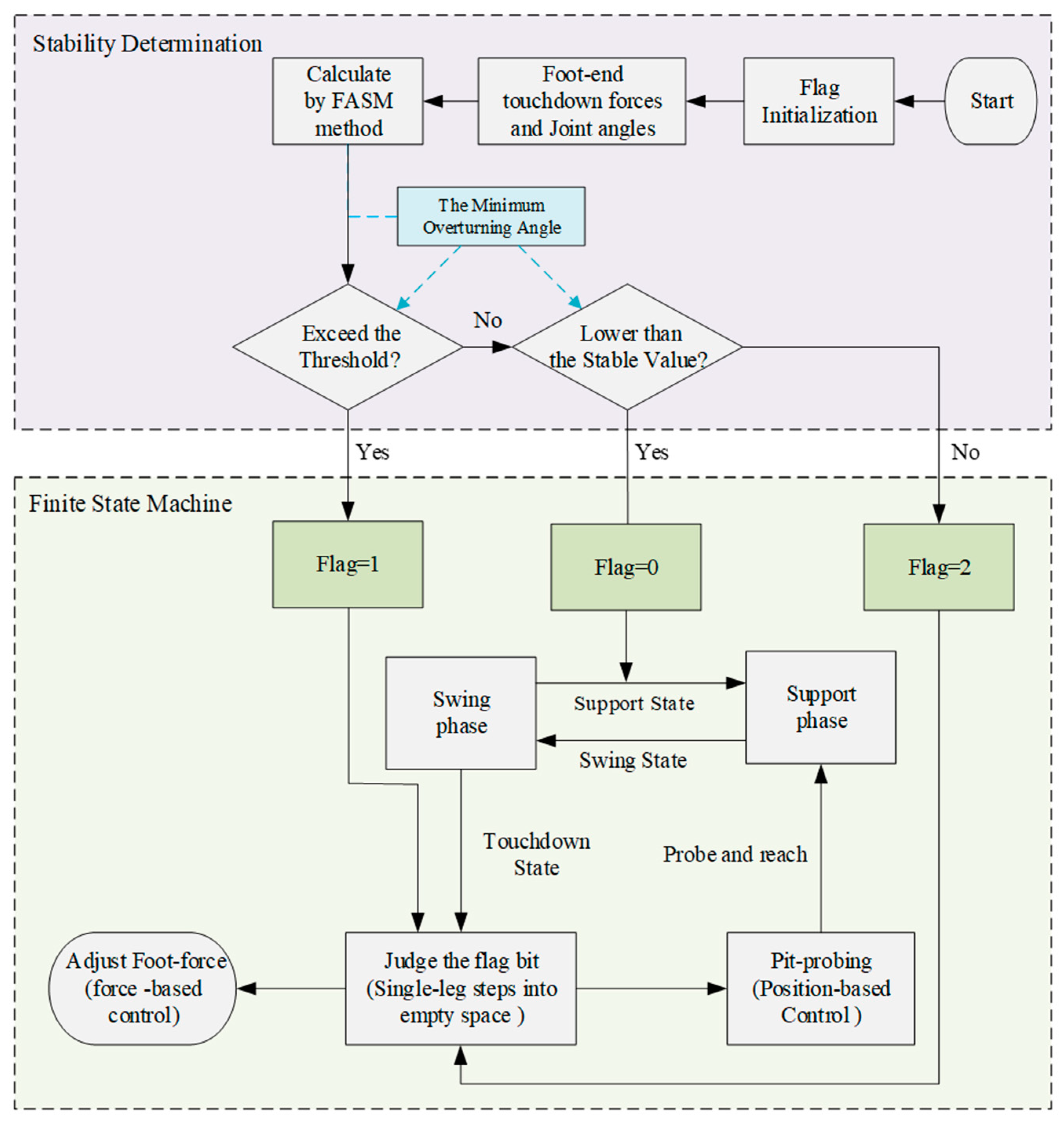
3. State Machine Strategy Based on FASM Stabilization Criterion

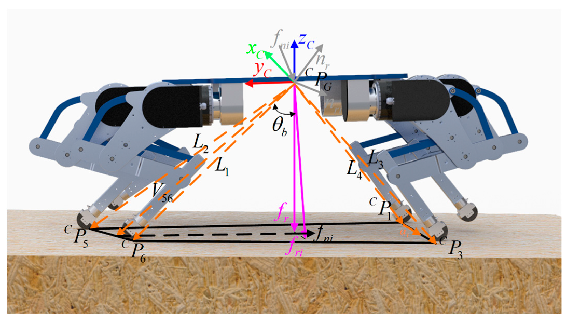
3.1. Robot Tipping and Instability Determination

When the hexapod robot walks in the quadrupedal gait, it is subjected to the action of gravity, inertial force, external disturbance force, and foot-end touchdown force. According to the Alembert principle, by conducting the dynamic analysis of the hexapod robot, the force and moment balance equations can be obtained as follows:

$${\displaystyle \sum f_{gra}+{\displaystyle \sum f_{iner}+{\displaystyle \sum f_{con}+{\displaystyle \sum f_{ext}}}}}=0$$

(9)

$${\displaystyle \sum f_{gra}+{\displaystyle \sum f_{iner}+{\displaystyle \sum f_{con}+{\displaystyle \sum f_{ext}}}}}=0$$

(10)

where $f_{grav}$, $n_{grav}$ are the gravitational force of the robot and the moment generated by gravity, respectively; $f_{iner}$, $n_{iner}$ are the inertial force and inertial moment, respectively; $f_{con}$, $n_{con}$ are the contact force and contact moment between the foot-end and the ground, respectively; and $f_{ext}$, $n_{ext}$ are the external disturbance force and disturbance moment, respectively. By transforming the above formula, the resultant force and resultant moment that cause the robot to become unstable are obtained as follows:

$$f_r={\displaystyle \sum f_{grav}+{\displaystyle \sum f_{ext}+{\displaystyle \sum f_{iner}=-{\displaystyle \sum f_{con}}}}}$$

(11)

$$n_r={\displaystyle \sum n_{grav}+{\displaystyle \sum n_{ext}+{\displaystyle \sum n_{iner}=-{\displaystyle \sum n_{con}}}}}$$

(12)

When the hexapod robot is in the motion state, the footholds of the legs in contact with the ground form a support polygon on the support surface. ${}^{C}P_i={[{}^{C}P_{ic},{}^{C}P_{iy},{}^{C}P_{iz}]}^T$ represent the position vector of the foothold $i$ in the body coordinate system. The lines connecting adjacent footholds are selected as the possible overturning axes of the body to form the support polygon. The overturning axis $i$ is denoted as:

$$\left\{\begin{array}{l}{a}_i={}^{C}P_{i+1}-{}^{C}P_i\\ a_k={}^{C}P_1-{}^{C}P_k\end{array}\right.,i=1,2\dots k-1$$

(13)

where $k$ is the number of feet in contact with the ground. Normalize the rotation axis vector to get ${\widehat{a}}_i=a_i/‖a_i‖$; further analyze the projection of the resultant force $f_r$ in the unstable state onto the plane with $\widehat{\alpha }$ as the normal vector:

$$f_{ri}=(E-{\widehat{\alpha }}_i{{\widehat{\alpha }}_i}^T)f_r$$

(14)

The component of the equivalent resultant moment $n_r$ at the center of gravity of the hexapod robot in the $\widehat{\alpha }$ direction is $n_{ri}$, and $f_{ri}$, $n_{ri}$ are the resultant force and resultant moment that cause the hexapod robot to tip over along the axis ${\widehat{a}}_i$. The schematic diagram of the stability cone of the support polygon during the quadrupedal gait of the robot is shown in Figure 3. ${}^{C}P_G-{}^{C}P_1{}^{C}P_3{}^{C}P_6{}^{C}P_5$ is the constructed stability cone of the hexapod robot. The vector passing through the center of gravity of the robot and perpendicular to the side $i$ of the support polygon is $V_i=(E-{\widehat{a}}_i{{\widehat{a}}_i}^T)({}^{C}P_{i+1}-{}^{C}P_G)$. After normalization, it is represented by ${\widehat{V}}_i$, and the equivalent couple in the support plane for the side line ${\widehat{a}}_i$ of the support polygon is:

$$f_{ni}={\displaystyle \frac{{\widehat{V}}_i\times n_{ri}}{‖V_i‖}}$$

(15)

The resultant overturning force $f_i^{\ast }$ at the center of gravity of the hexapod robot with respect to the support polygon $i$ is:

$$f_i^{\ast }=f_{ri}+f_{ni}$$

(16)

Normalizing $f_i^{\ast }$, it can obtain ${\widehat{f}}_i^{\ast }$. The overturning angle of the side line ${\theta }_{bi}$ can be calculated by $V_i$ and $f_i^{\ast }$. The stability margin in the FASM method is defined as the minimum value of the included angles of each side, that is,

$$S_{FASM}=\underset{i=1}{\overset{k}{\min }}({\theta }_{bi})$$

(17)

As the index to judge the stability of the hexapod robot, if the minimum overturning angle exceeds the threshold, the flag bit Flag = 1; if its value is lower than the stable value, Flag = 0; in other cases, Flag = 2.

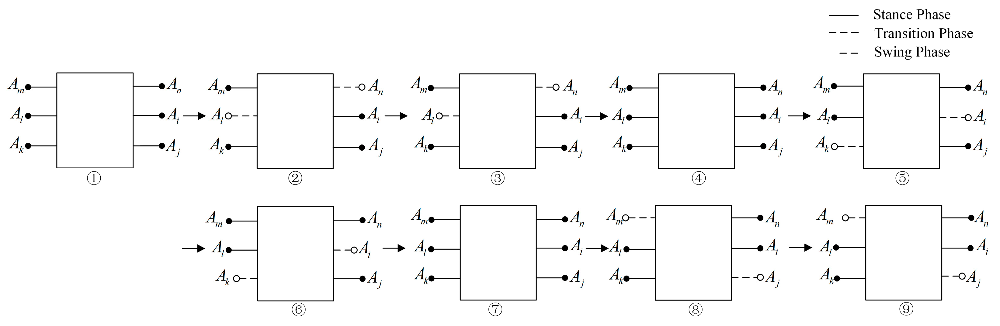
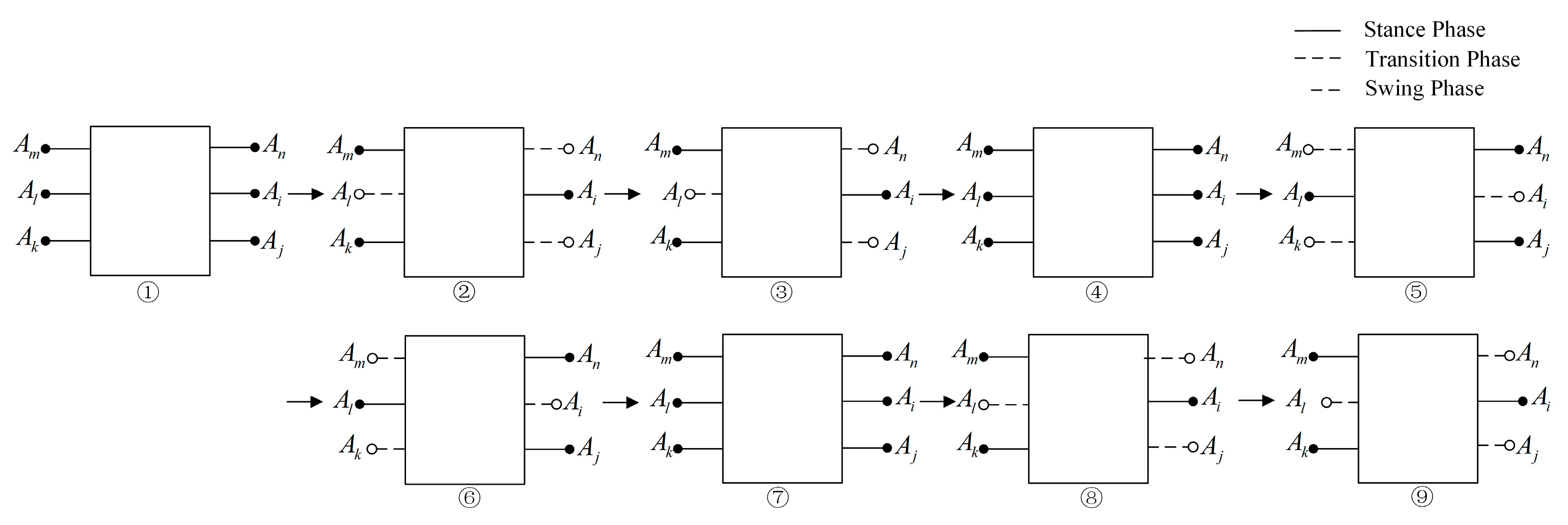
3.2. Finite State Machine Design

When moving in a complex dynamic environment, the phase of each leg of the hexapod robot is programmed by its planner and controller based on a predefined gait sequence. However, generating phases solely based on time is an idealized assumption that struggles to accommodate the unstructured variations of real terrain. During locomotion, the legs may prematurely touch the ground due to obstacles or experience delayed contact due to foot misplacement, affecting gait stability. To address this issue, this paper proposes a finite state machine control strategy triggered by foot-end touchdown events, enabling rapid response and dynamic adjustment to unexpected situations such as foot misplacement and slipping.

To achieve smooth switching between different states of the hexapod robot, it is necessary to comprehensively consider the leg force feedback, the flag bit of the finite state machine, and the time parameters of the swing phase and the support phase to determine whether to switch the state. The flowchart of the finite state machine is shown in Figure 4.

This process mainly includes the following stages:

(1)

Swing state: When the foot end enters the swing phase, execute the desired trajectory tracking.

(2)

Support state: When the foot end enters the support phase, if the value measured by the force sensor is greater than the set value and Flag = 0, it is determined to be in a stable support state.

(3)

Empty-stepping state: When the foot end enters the support phase, if the force feedback suddenly changes and is lower than the set value, it is determined as empty-stepping, and corresponding decisions are triggered according to the flag bit.

(4)

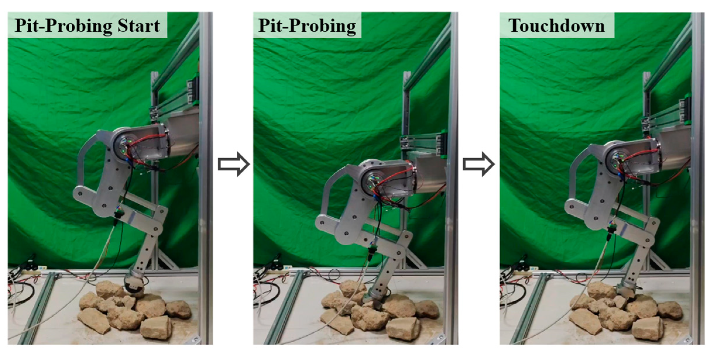
Pit-probing state: In the empty-stepping state, if the finite state machine flag bit Flag = 2, the leg adopts admittance control to make the foot end probe the bottom of the pit along the preset trajectory and land on the ground.

(5)

Foot-force adjustment state: In the empty-stepping state, if the flag bit Flag = 1, the leg adopts force-based impedance control to adjust the force exerted by the foot end to reduce the impact.

The flow chart of the finite state machine is shown in Figure 4.

Figure 5 shows the support-phase polygon, which ensures that the center of gravity of the hexapod robot remains stable even when a touchdown leg steps into an empty space [21]. Figure 6 illustrates the schematic diagram of the robot’s quadrupedal gait. Number 1 represents the initial state of the gait; in number 2, two legs marked with black dots enter the swing phase. After completing the swing, number 3 shows the new support state. Number 4 indicates that the robot has returned to six-leg support. Subsequently, the robot continues alternating between support and swing phases according to the predetermined gait pattern. According to the minimum tipping angle and the judgment of the finite state machine, the leg that steps into the empty space can adjust the foot-end displacement through admittance control. While achieving local contact and detection, it can also adjust the normal force at the contact point, thereby improving the walking stability of the robot on collapsible terrains.

Figure 7 illustrates the instability that occurs during the tripod gait when a touchdown leg steps into an empty space. In this case, the footholds of the support legs cannot form a support-phase polygon, causing the hexapod robot to tip over and enter a free-fall state. To address this issue, the force-based impedance control method is adopted to reduce foot-end impact, and relevant vertical dynamics indicators [22] are used to evaluate the effectiveness of this method. Figure 8 illustrates the schematic diagram of the robot’s triangular gait. Number 1 represents the initial state of the gait; in number 2, three legs marked with black dots enter the swing phase. After completing the swing, number 3 shows the new support state. Number 4 indicates that the robot has returned to six-leg support. Subsequently, the robot continues alternating between support and swing phases according to the predetermined gait pattern.

4. Design of Pit-Probing Control Based on Admittance Control Method

4.1. Admittance Control Method

The core idea of admittance control is to take the deviation between the desired force and the foot-end touchdown force as the input to the impedance controller, which then generates a position correction amount. The target position of the foot-end is dynamically adjusted to achieve the force control effect. This control method is usually described by a second-order differential model:

$$F_r-F_{gnd}=M_d({\ddot{x}}_d-{\ddot{x}}_a)+B_d({\dot{x}}_d-{\dot{x}}_a)+K_d(x_d-x_a)$$

(18)

where $F_{gnd}$ is the foot-end touchdown force; $F_r$ is the foot-end desired force; $M_d$ is the inertia parameter of the impedance controller; $B_d$ is the damping parameter; $K_d$ is the stiffness parameter; $x_d$, ${\dot{x}}_d$, ${\ddot{x}}_d$ are the desired position, velocity, and acceleration, respectively, during the motion of the single leg; and $x_a$, ${\dot{x}}_a$, ${\ddot{x}}_a$ are the actual position, velocity, and acceleration, respectively, during the motion of the single leg. Define $\Delta x$ as the displacement deviation at the foot-end, and $\Delta x=x_d-x_a$; then, the impedance control equation can be simplified as follows:

$$F_r-F_{gnd}=M_d\Delta \ddot{x}+B_d\Delta \dot{x}+K_d\Delta x$$

(19)

The schematic based on the admittance control principle is shown in Figure 9. Where $F_{gndx}$ is the horizontal force exerted by the external environment on the foot-end; $F_{gndy}$ is the vertical force exerted by the external environment on the foot-end; $\Delta x$ and $\Delta y$ are the position correction amounts in the horizontal and vertical directions of the foot-end, respectively; and $\Delta F=F_r-F_{gnd}$.

Although admittance control has a certain lag, it features simple calculations and does not require a complex dynamic model, and it offers relatively high precision in position control of the foot-end. In contrast, force-based impedance control has relatively lower control precision, but it can directly adjust the contact force, thus providing better compliance.

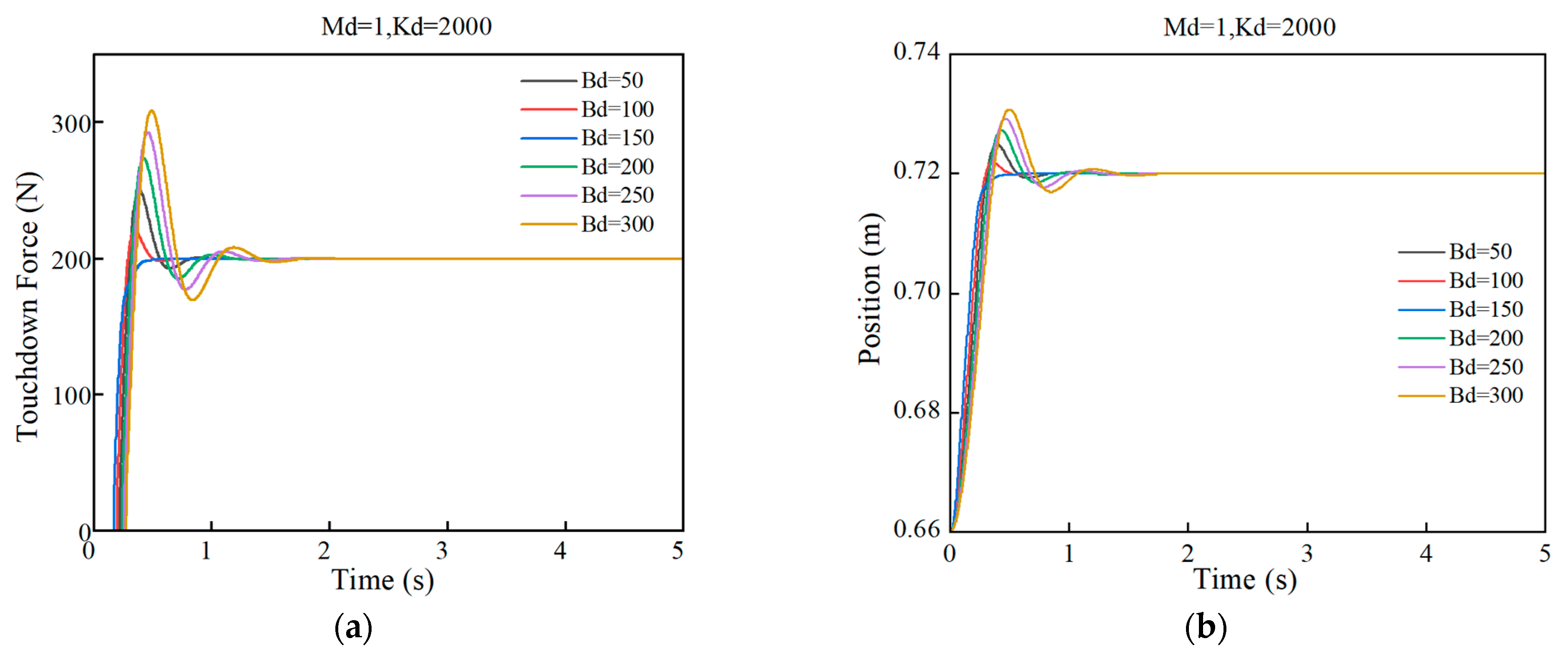
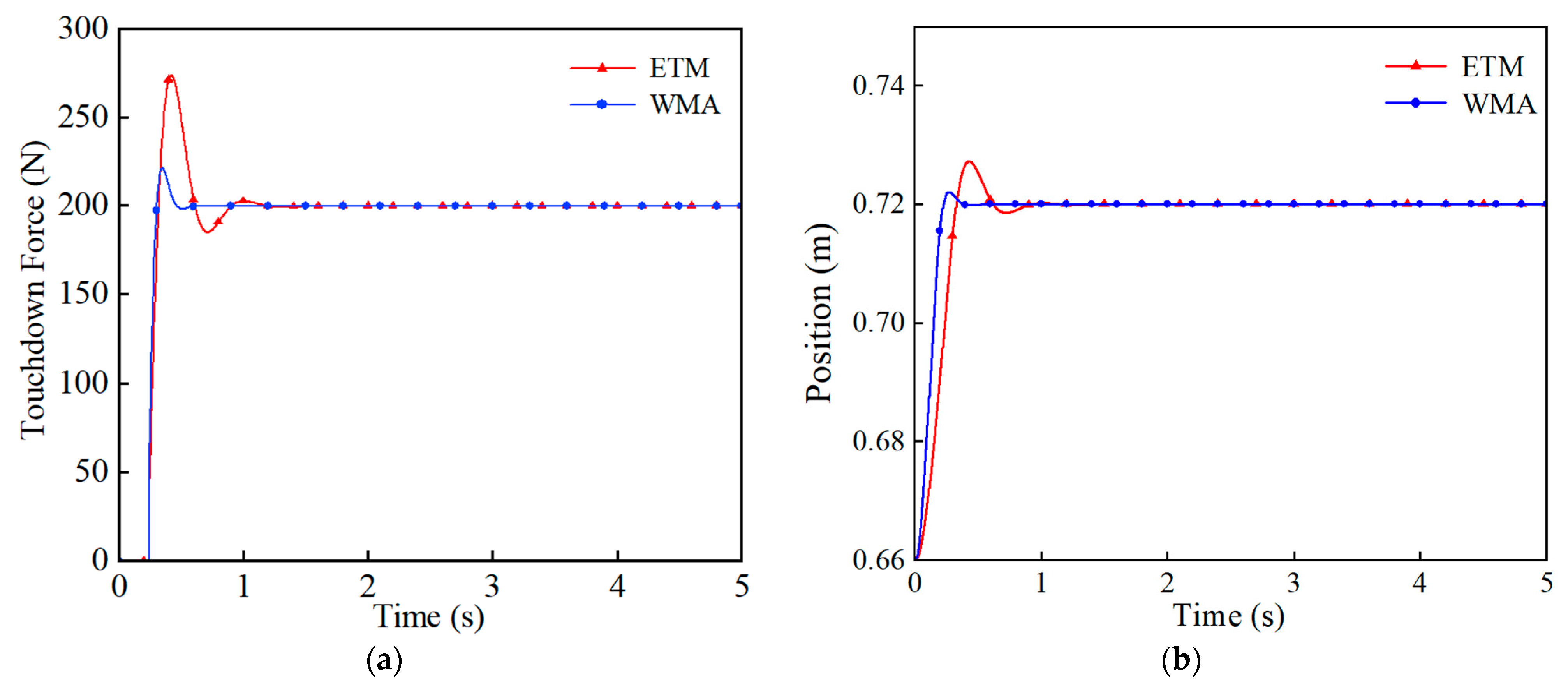
4.2. Comparison of Control Effects of Impedance Optimization Parameters

The impedance parameters of the single leg directly affect the control effect, so it is difficult to obtain optimal results using the traditional empirical tuning method. Therefore, optimizing the impedance parameters by an optimization algorithm is necessary. The whale migration algorithm (WMA) [23] is a global optimization algorithm that simulates the migration and predation behaviors of humpback whales. It has the characteristics of diverse populations, simplicity, and flexibility. The process of WMA for impedance parameter optimization is as follows:

(1) Initialization of whale positions

At the initial stage of the algorithm, a set of whale positions needs to be randomly generated in the search space. Assume that the position vector of a whale is

$$W_i=L+rand(1,D)\odot (U-L),i=1,2\dots ,N_{pop}.$$

where:

$L=(L_1,L_2,\dots L_D)$ is the lower bound vector of the search space.

$U=(U_1,U_2,\dots ,L_D)$ is the upper bound vector of the search space.

$rand(1,D)$ is a D-dimensional random vector whose elements are in the range of [0, 1]; $\odot$ represents the Hadamard product (element-wise product); and $N_{pop}$ is the size of the whale population.

(2) Selection of the leader

In each generation, the whales are sorted according to their fitness values. The whale with the best fitness value is selected as the leader. Assume that the position of the leader is $W_{B\mathrm{est}}$; its fitness value is $f(W_{B\mathrm{est}})$.

(3) Update of whale positions

The update of whale positions is divided into two parts: the position update of followers and the position update of the leader.

(a) Position update of followers:

For each follower whale $W_i$, the position update formula is:

$$W_i^{new}=W_{Mean}+rand(1,D)\odot (W_{i-1}-W_i)\odot (W_{Best}-W_{M\mathrm{ean}})$$

where $W_{Mean}$ is the average of the positions of all current leader whales, and its calculation formula is:

$$W_{M\mathrm{ean}}={\displaystyle \frac{1}{N_L}}{\displaystyle \sum _{j=1}^{N_L}{W}_j}$$

where $N_L$ is the number of leader whales, and $W_{i-1}$ is the position of the whale preceding the follower whale $W_i$.

(b) Position update of the leader:

For each leader whale $W_i$, the position update formula is:

$$W_i^{new}=W_i+rand(1,D)\odot L+rand(1,D)\odot (U-L)$$

where $L$ and $U$ is the lower bound and upper bound vectors of the search place, respectively; and $rand(1,D)$ is a D-dimensional random vector whose elements are in the range of [0, 1].

(4) Boundary handling

When updating the whale positions, it is necessary to ensure that the new position $W_i^{new}$ still lies within the search space. If $W_i^{new}$ exceeds the boundaries, project it back onto the search space.

$$W_i^{new}=\max (L,\min (W_i^{new},U))$$

(5) Calculation of fitness values

In each generation, calculate the fitness value $f(W_i^{new})$ of the position of each whale. If the fitness value of the new position is better than that of the current position, update the position:

$$f(W_i^{new})\le f(W_i),W_i=W_i^{new}$$

(6) Iteration termination condition

The algorithm automatically terminates when it reaches the maximum number of iterations or meets other stopping conditions and returns the position $W_{B\mathrm{est}}$ of the optimal whale as the optimal solution, that is, the optimal parameters of impedance. The fitness curve of this algorithm is shown in Figure 10. The simulation results show that the algorithm converges to a good fitness value within a small number of iterations, which verifies its excellent optimization performance.

To evaluate the parameter optimization effect of the WMA, this paper constructs an impedance control model. The empirical tuning method (ETM) and the WMA are used for parameter tuning to compare their control performances. For the parameters $M_d\in [0,11]$, $B_d\in [0,300]$, $K_d\in [0,3000]$ obtained by the ETM, the system is tuned, and the influence of parameter changes on the contact force and position error is analyzed. The simulation results are shown in Figure 11, Figure 12 and Figure 13.

According to the patterns shown in the figures, two groups of parameter optimization experiments are carried out using the ETM and the WMA algorithm, respectively. The final results of the optimized parameters are shown in

Table 1. Optimized parameters.

Optimization Method	${\mathit{M}}_{\mathit{d}}$	${\mathit{B}}_{\mathit{d}}$	${\mathit{K}}_{\mathit{d}}$
ETM	1	200	2000
WMA	0.5	60	1500

.

Based on the above two sets of optimal parameters, simulation experiments are carried out respectively. The comparison results are shown in Figure 14.

4.3. Simulation Based on Admittance Control

The motion simulation of the single leg based on admittance control was carried out in the Simulink simulation environment. The stiffness parameter of the contact ground was set as $2\times {10}^4$, the damping parameter as $3\times {10}^4$, and the gravitational acceleration as $9.8\mathrm{m}/{\mathrm{s}}^2$. The single leg was placed above the ground at a certain height to perform ground detection according to the preset trajectory until it made contact with the ground, and the process of pit-probing after stepping into empty space was simulated, as shown in Figure 15.

Simulations were conducted on the non-impedance control, the admittance control, the ETM, and the WMA, respectively. The control effects of the three methods on the change of normal touchdown force over time were compared, and the results are shown in Figure 16.

As shown in Figure 14, without using impedance control, the maximum contact force at the foot end was 620 N. After optimizing the impedance parameters using the ETM, the maximum contact force dropped to 280 N. By further optimizing the parameters with the WMA, the maximum contact force decreased to 230 N, which verifies the effectiveness of the impedance control and the parameter optimization algorithm.

5. Design of Force-Based Impedance Control for Foot Cushioning

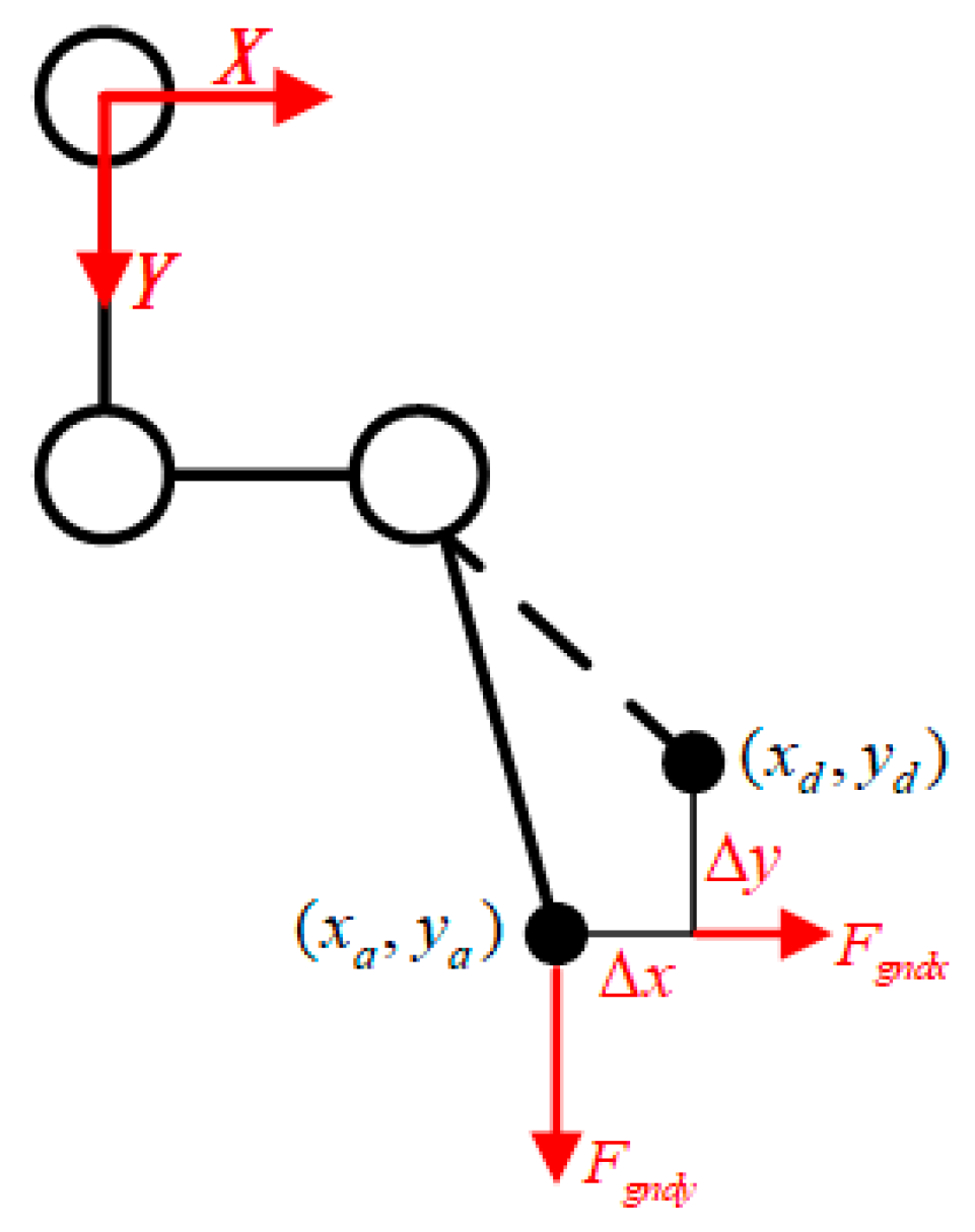
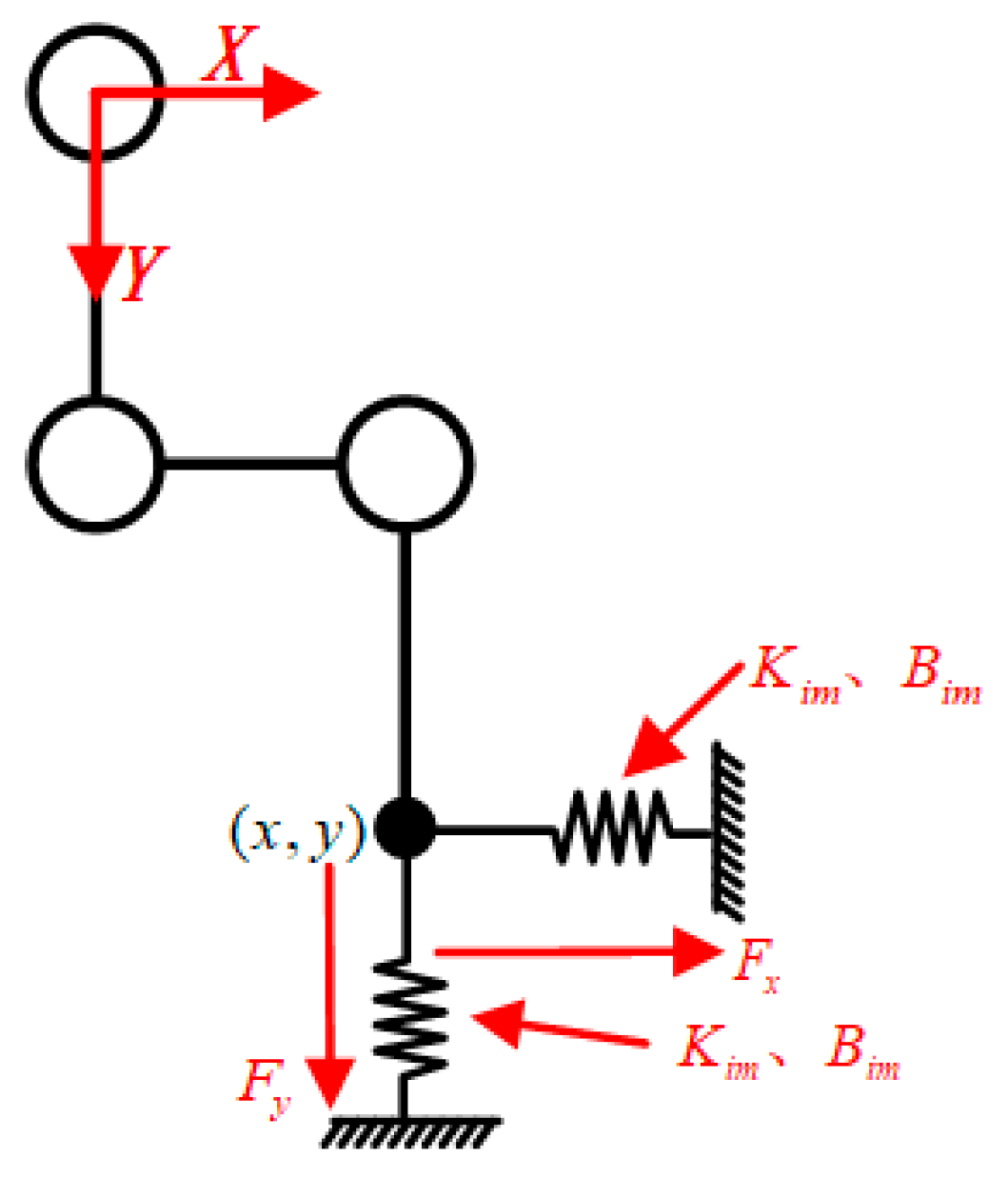
5.1. Force-Based Impedance Control Design

When the robot lands on the ground, the dynamic form of the external force acting on the foot-end can be expressed as:

$$\tau =M(\theta )\ddot{\theta }+V(\theta ,\dot{\theta })+G(\theta )+J^T(\theta )F_e$$

(20)

where $\tau$ is the input driving torque of the hexapod robot; $F_e$ is the force at the end-effector of the hexapod robot; and $J^T$ is the transpose of the force Jacobian matrix of the hexapod robot.

In force-based impedance control, the system calculates the expected output force at the foot-end through the impedance controller based on the deviation between the target position and the actual position of the foot-end. The schematic diagram of the principle of force-based impedance control for the single leg is shown in Figure 17.

When the single leg is in motion, the control force at the foot-end can be described as:

$$F_{im}=M_{im}({\ddot{X}}_d-\ddot{X})+B_{im}({\dot{X}}_d-\dot{X})+K_{im}(X_d-X)$$

(21)

where $F_{im}$ is the impedance output force; $M_{im}$ is the inertia parameter; $B_{im}$ is the damping parameter; $K_{im}$ is the stiffness parameter; $X_d$, ${\dot{X}}_d$, ${\ddot{X}}_d$ are the desired position, desired velocity, and desired acceleration of the foot-end of the hexapod robot, respectively; and $X$, $\dot{X}$, $\ddot{X}$ are the actual position, actual velocity, and actual acceleration of the foot-end of the hexapod robot, respectively. In practical applications, since the second-derivative term $\ddot{x}$ of the actual position of the foot-end is greatly affected by noise, to reduce the system oscillation caused by the excessive feedback torque at the moment of impact, the acceleration term in the impedance model is usually ignored in practice, and the following expression is adopted:

$$F_{im}=B_{im}({\dot{X}}_d-\dot{X})+K_{im}(X_d-X)$$

(22)

$$F_{fl}=\widehat{C}(X,\dot{X})\dot{X}+\widehat{G}(X)$$

(23)

The gravity vector $\widehat{G}(X)$ is easier to calculate than the mass matrix, and the calculation of the Coriolis and centrifugal forces $\widehat{C}(X,\dot{X})$ is more complex than that of the mass matrix and the gravity vector. In the closed-loop system of Equation (16), the corrected torque is added through feedback. The simplest form of the inverse dynamics control output, which can be calculated from the Coriolis and centrifugal force matrix and the gravity vector in the dynamic model, includes the following two terms:

$$F=F_{im}+F_{fl}$$

(24)

$$F_{fl}=\widehat{G}(X)$$

(25)

To ensure zero steady-state error in trajectory tracking, it is only necessary to have full knowledge of the gravity term and calculate the mass matrix. Therefore, there is no need to consider the Coriolis and centrifugal force matrix in the feedback. Compared with the general inverse dynamics control method, the computational load of this method is significantly reduced.

5.2. Stability Analysis of the Control System

Force-based impedance has stronger compliance. The asymptotic tracking ability of its control strategy is verified through the Lyapunov method [24]. The overall energy of the closed-loop system is selected as the candidate Lyapunov function:

$$V={\displaystyle \frac{1}{2}}{\dot{X}}^{T}M\dot{X}+{\displaystyle \frac{1}{2}}{e}_x^T{K}_{im}{e}_x$$

(26)

This equation includes the kinetic energy of the leg and the potential energy that generates the proportional feedback term $K_{im}{e}_x$. Therefore, $V(X)$ is a positive value throughout the entire workspace of the leg, except when the hexapod robot reaches the desired position, $X=X_d$, $\dot{X}=0$, and the Lyapunov $V=0$. The Lyapunov stability requires that the time derivative of the $V(X)$ along the motion trajectory of robot is negative definite. If this condition is satisfied for all motion trajectories, it means that the total energy of the robot approaches zero. Moreover, since the energy can only be zero when its trajectory converges to the desired trajectory, it indicates that the single leg can achieve asymptotic tracking. For the case where the desired trajectory is constant, the derivative of the Lyapunov function can be expressed as:

$$\dot{V}={\dot{X}}^{T}M\ddot{X}+{\displaystyle \frac{1}{2}}{\dot{X}}^T\dot{M}\dot{X}+{\dot{e}}_x^T{K}_{im}{e}_x$$

(27)

Substitute $M\ddot{X}$ from the dynamic into the Equation (27). Since the desired trajectory is constant, ${\dot{X}}_d=0$. Therefore, the derivative of the Lyapunov function can be simplified as:

$$\dot{V}={\dot{X}}^T(F_{im}+F_{fl}-C\dot{X}-G)+{\displaystyle \frac{1}{2}}{\dot{X}}^T\dot{M}\dot{X}+{\dot{e}}_x^T{K}_{im}{e}_x={\dot{X}}^T(K_{im}{e}_x+B_{im}{\dot{e}}_x-C\dot{X})+{\displaystyle \frac{1}{2}}{\dot{X}}^T\dot{M}\dot{X}+{\dot{e}}_x^T{K}_{im}{e}_x$$

(28)

Since the desired trajectory ${\dot{X}}_d=0$, ${\dot{e}}_x=({\dot{X}}_d-\dot{X})=-\dot{X}$, and Equation (27) can be simplified as:

$$\dot{V}=-{\dot{X}}^T{B}_{im}\dot{X}+{\displaystyle \frac{1}{2}}{\dot{X}}^T(\dot{M}-2C)\dot{X}=-{\dot{X}}^T{B}_{im}\dot{X}\le 0$$

(29)

This simplified result indicates that the derivative of the Lyapunov function is negative semi-definite, which cannot guarantee the achievement of asymptotic tracking.

To further explore the stability of the system, the LaSalle theorem is used to verify its asymptotic convergence. If $\dot{X}$ is non-zero and the $V$ is decreasing, that means the leg can reach a state where $\dot{X}=0$, but $X\ne X_d$. To prove that this situation will not occur, in which case $\dot{V}\equiv 0$, from Equation (28), we can obtain that $\dot{X}\equiv 0$, and the closed-loop dynamic equation can be expressed as:

$$M(X)\ddot{X}+C(X,\dot{X})\dot{X}=B_{im}\dot{X}+K_{im}{e}_x$$

(30)

After simplification, it can be expressed as:

$$K_{im}{e}_x=0$$

(31)

This indicates that for any positive proportional gain of the controller, $e_x=0$. Therefore, according to the Lasalle theorem, it can be guaranteed that in the steady state $X=X_d$, the closed-loop system achieves asymptotic tracking.

5.3. Force-Based Impedance Control Simulation

Place the single leg on the ground at a certain height and let it freely fall from a height of h = 0.1 m, as shown in Figure 18. Simulate the impact caused by the single leg stepping into the void during the tripod gait and adopt force-based impedance control to mitigate the impact.

Consider the similarity between the impact force characteristics caused by the motion of the robot and the suspension vibration evaluation. This paper applies the impact characteristic indicators in the vehicle field to evaluate the effectiveness of the single-leg impedance in reducing the impact force. Taking the maximum impact force and maximum acceleration in vertical dynamics as the evaluation indicators, the effectiveness of the impedance control algorithm is verified through simulation.

Free-fall simulations of a single leg of the hexapod robot were conducted, including a normal free-fall simulation and another with the force-based impedance control method. Vertical dynamic indicators were used to evaluate the effectiveness of the impedance control. The simulation results are shown in Figure 19 and Figure 20.

As shown in Figure 18, the maximum impact force is approximately 1800 N without the introduction of impedance control, and the stabilization time is about 1.2 s. After adding the impedance, the maximum impact force drops to approximately 800 N, the response time is reduced to about 0.95 s, and there is no rebound phenomenon. Meanwhile, the maximum acceleration is reduced by approximately 54%. Therefore, impedance control effectively reduces the impact force and enhances the anti-interference ability.

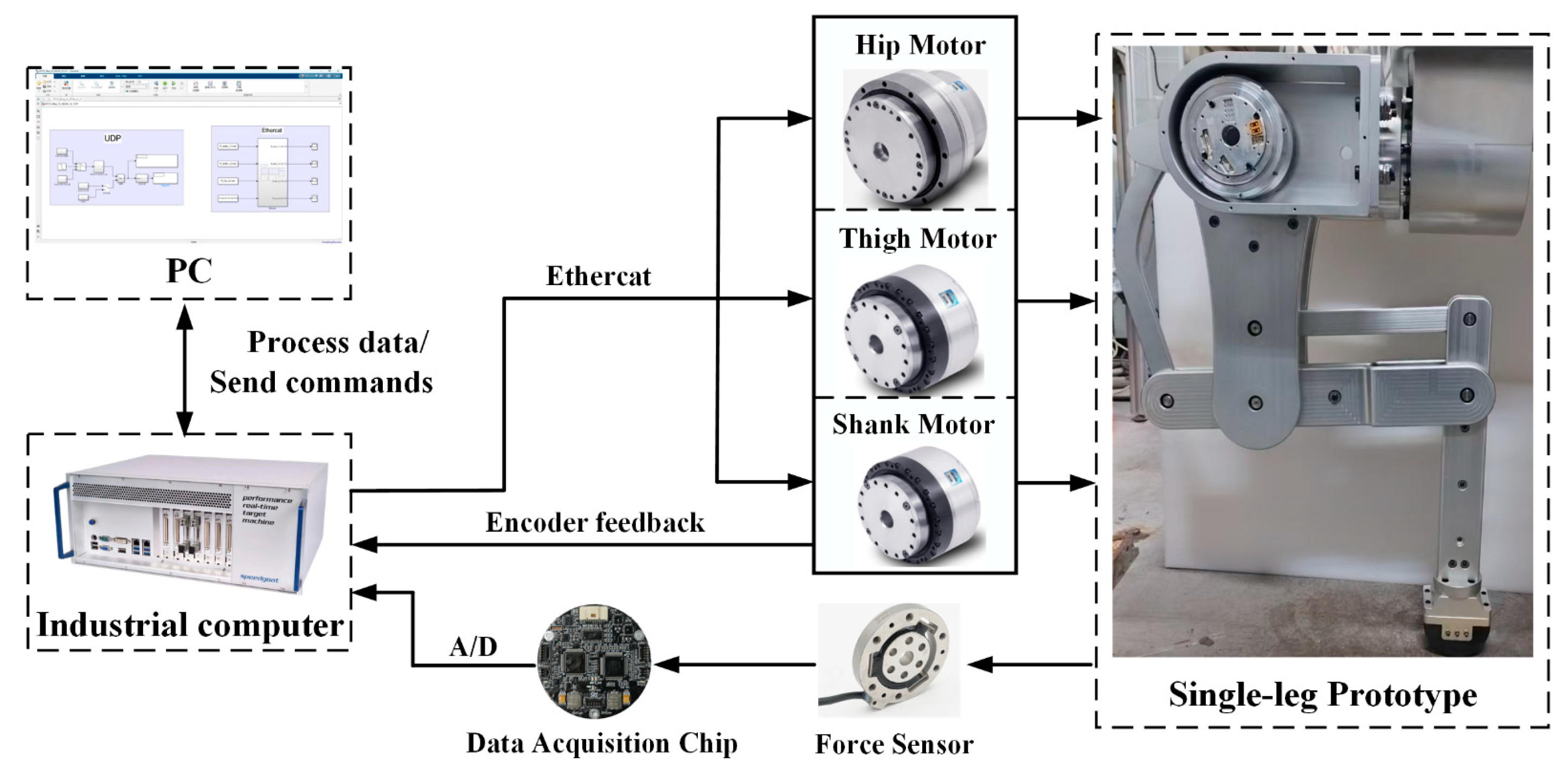
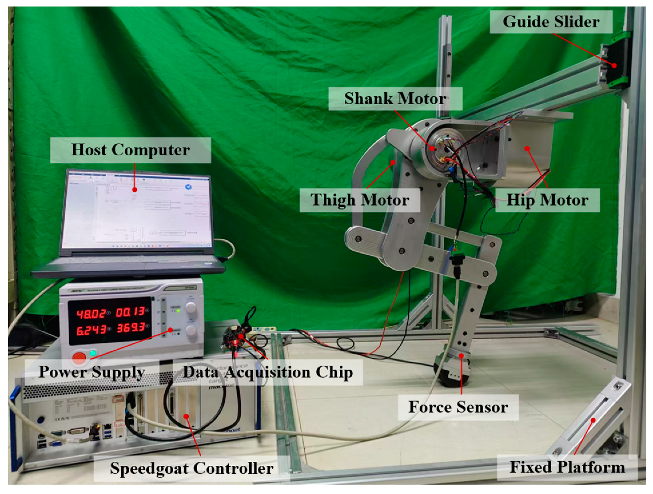
6. Prototype Experiment

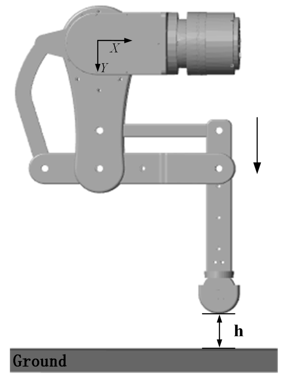
6.1. Experimental Scenario

The framework of the hardware platform for a single leg of the electrically driven hexapod robot is shown in Figure 21. The platform mainly consists of a structural base, a single-leg mechanism, an industrial computer, an adjustable power supply, and an SRI six-axis force sensor. The hip, thigh, and shank joints of the leg are actuated by integrated servo motors, each equipped with built-in 20-bit high-resolution encoders for precise joint angle measurement. These encoders form the basis for a closed-loop position and torque control system.

The control system is implemented in MATLAB/Simulink (2023a version) and executed in real time by the SpeedGoat controller, which serves as the slave computer. The host computer (a PC) communicates with the system via Simulink. The servo motors and the force sensor exchange data with the controller through EtherCAT and TCP protocols, respectively. The controller is manufactured by a company headquartered in Bern, Switzerland.

In this closed-loop system, sensor feedback is continuously used to adjust motor output, ensuring accurate tracking of desired joint trajectories and enabling real-time impedance control. This setup allows the robot leg to perform tasks such as impact simulations and pit-probing under controlled and repeatable conditions. The experimental setup is shown in Figure 22.

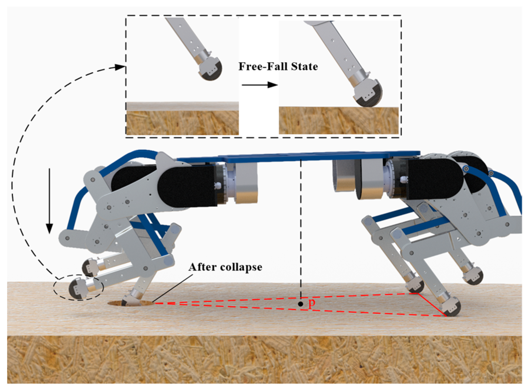
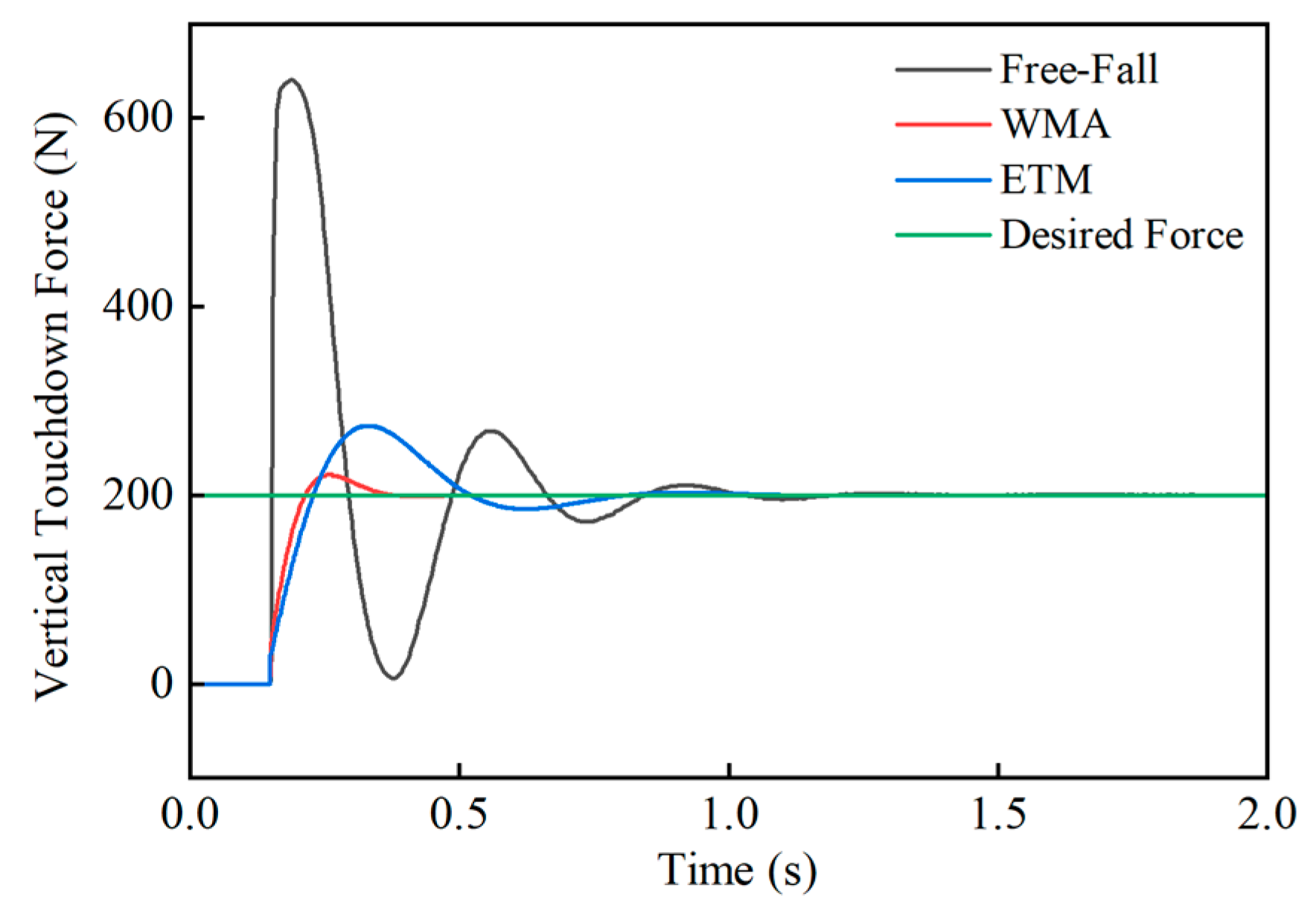
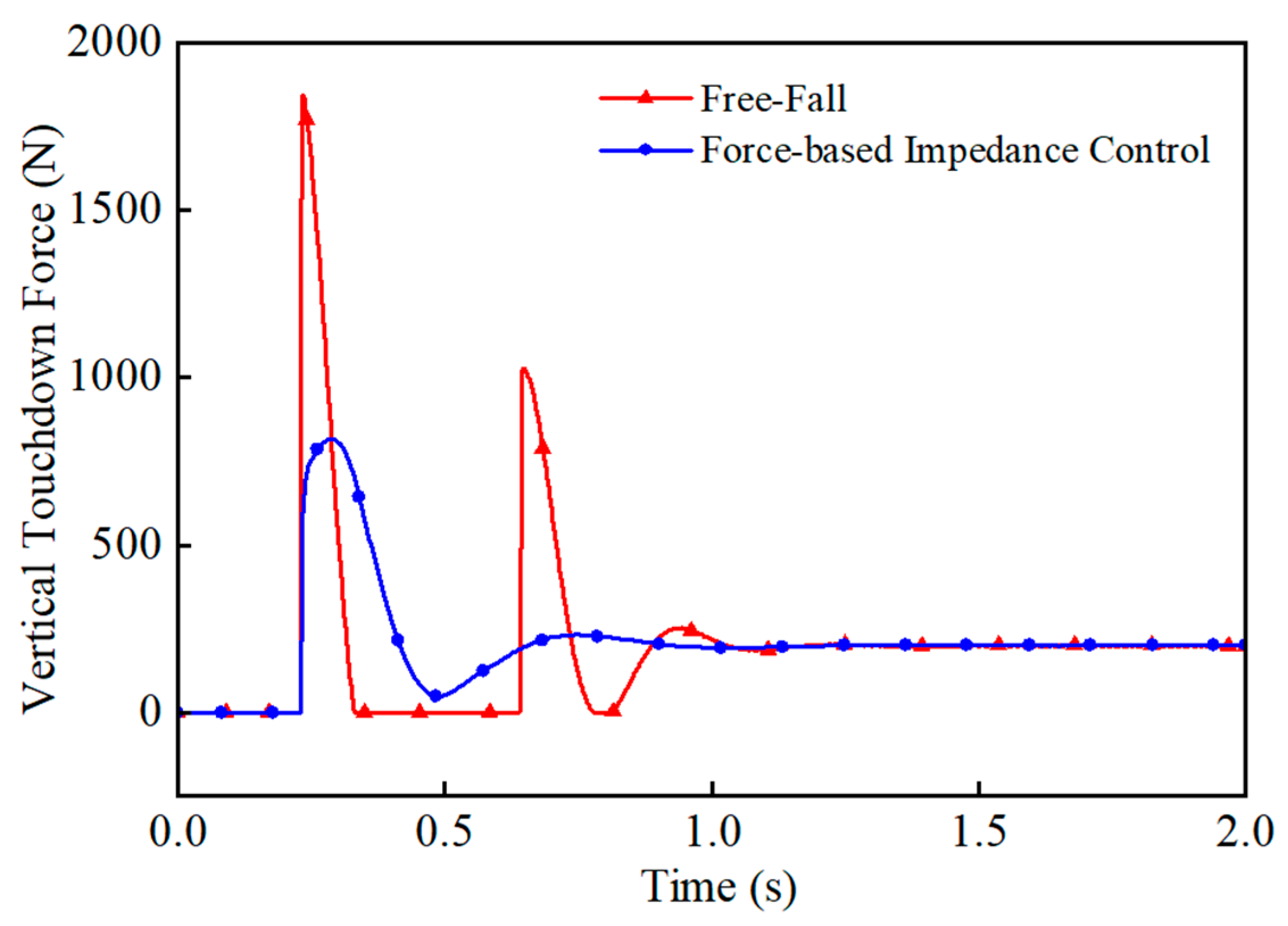
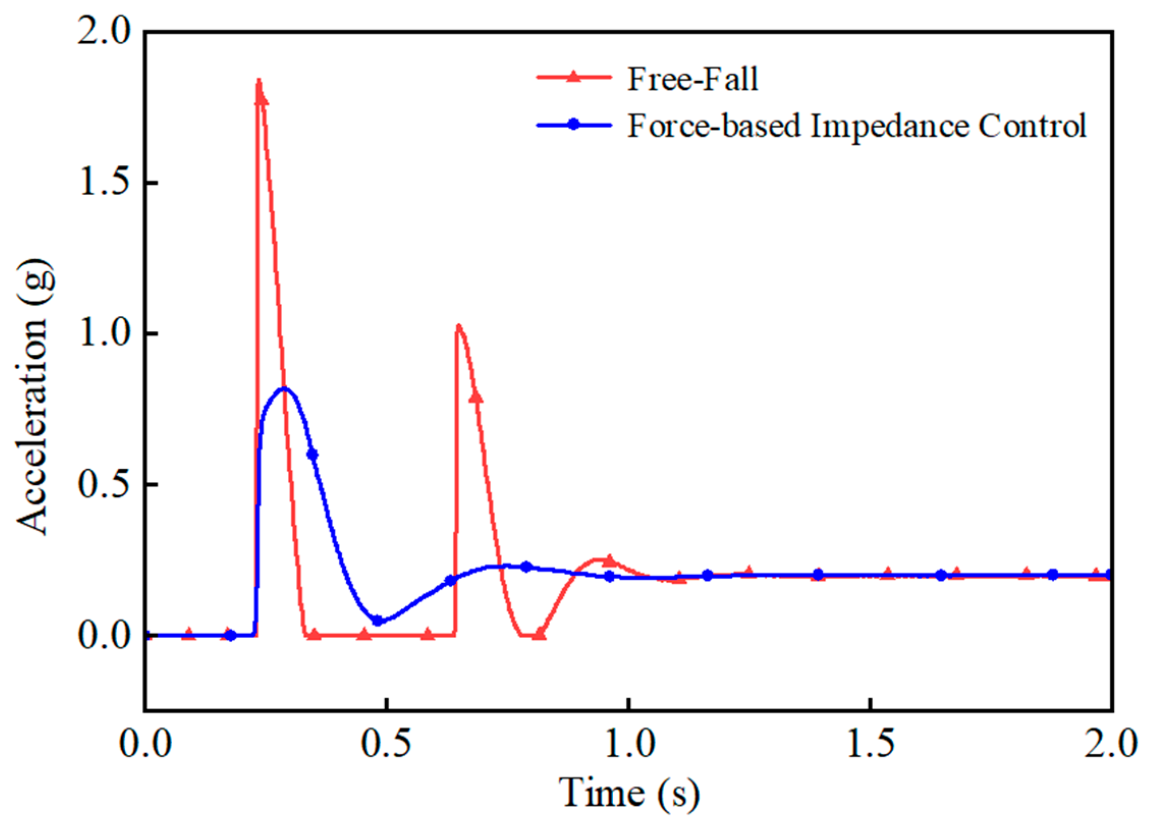
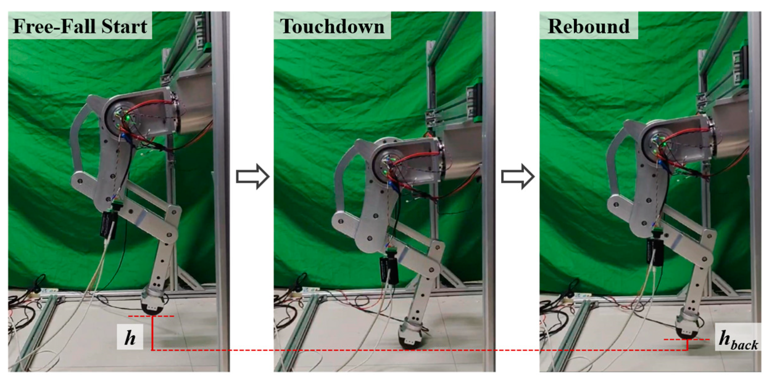
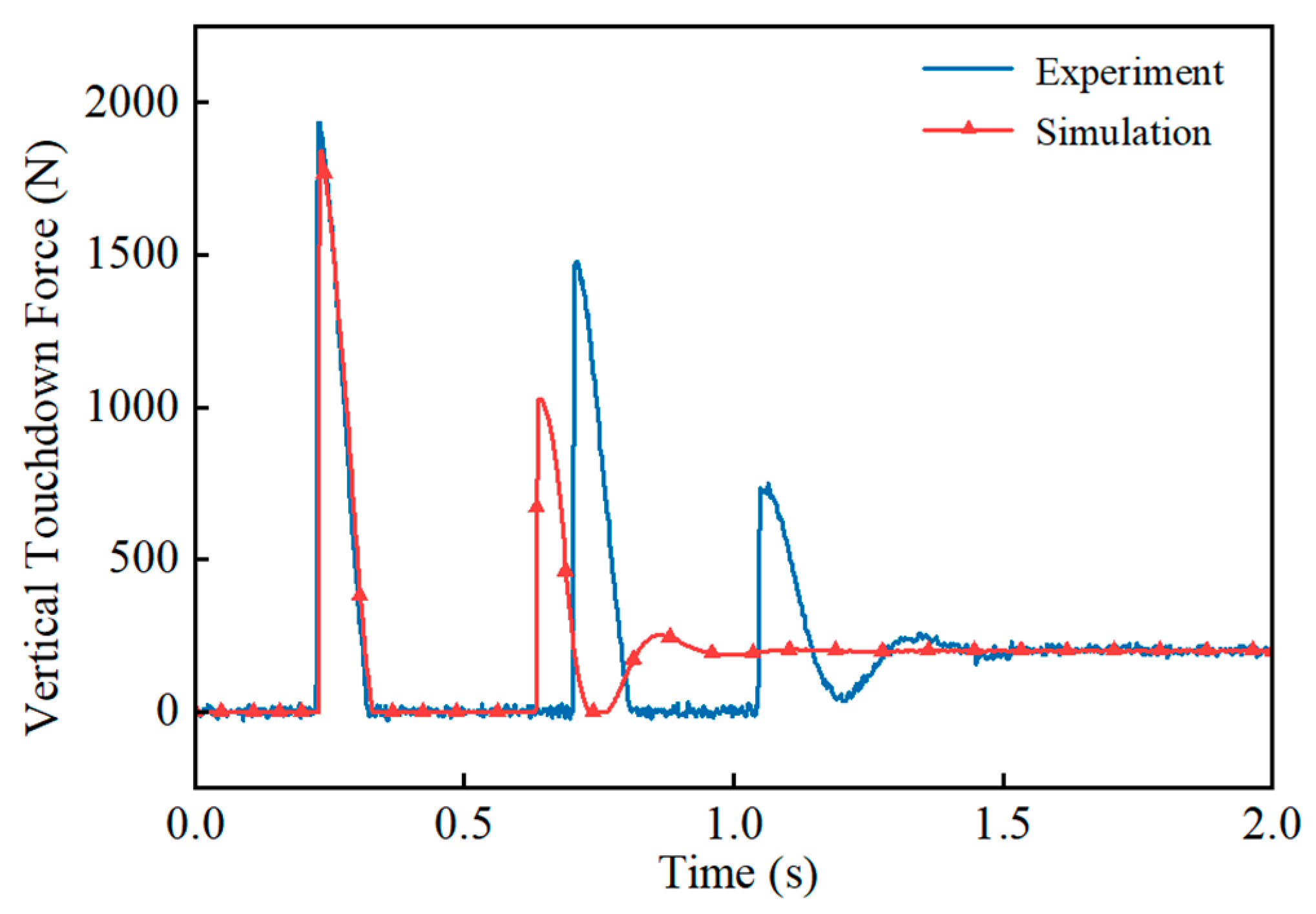
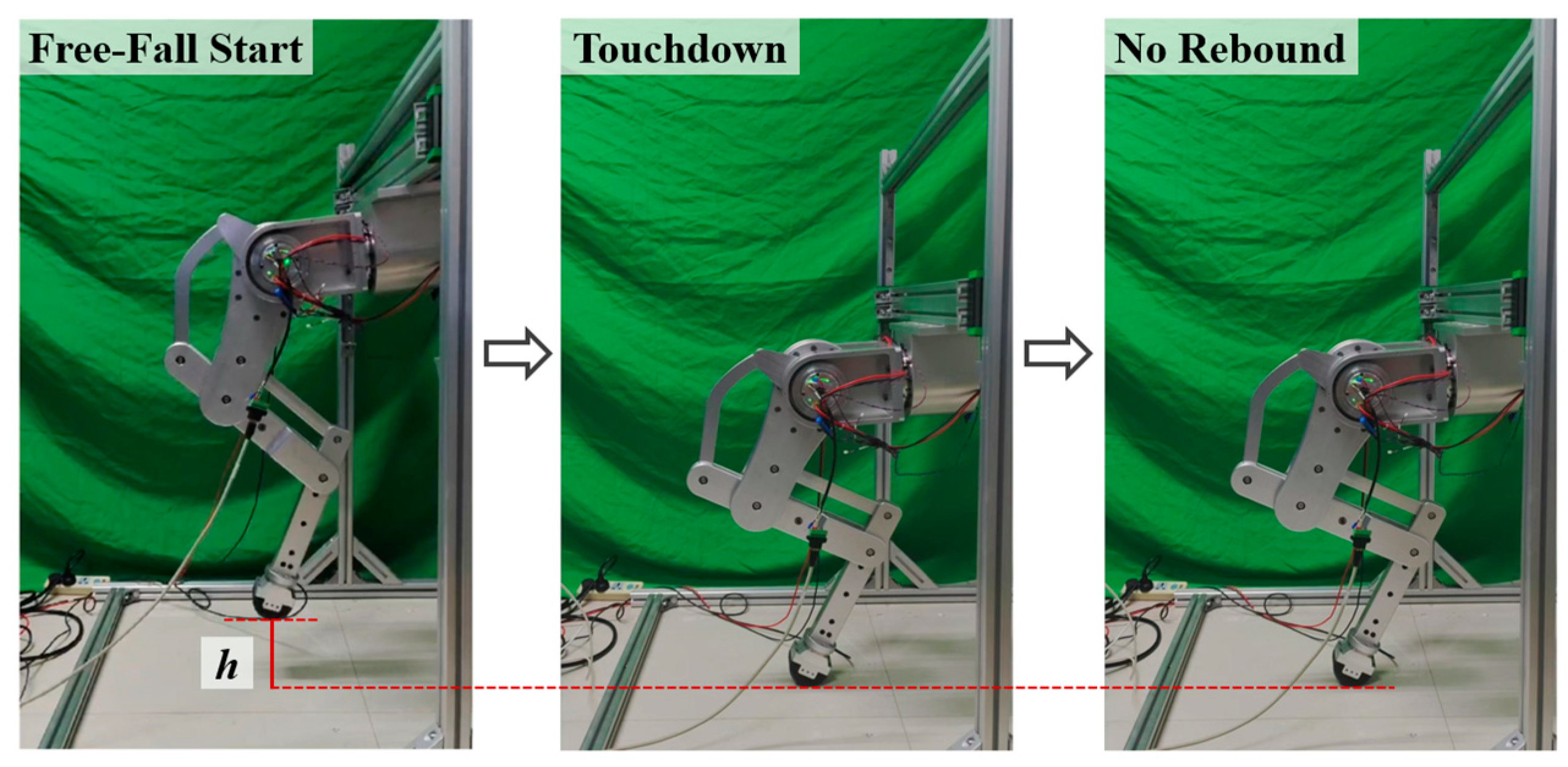
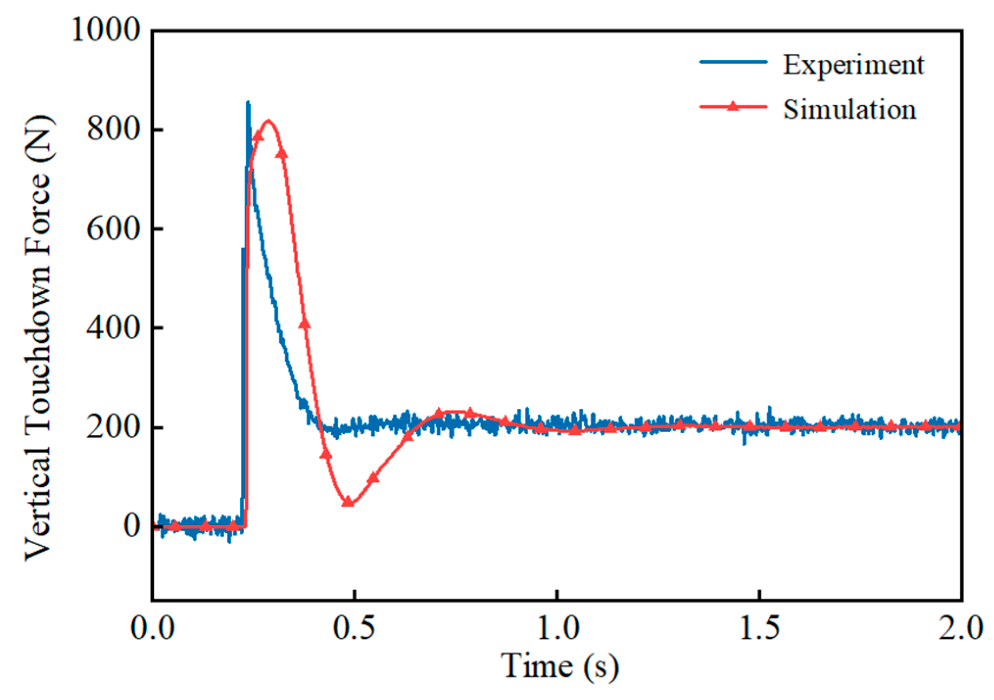
6.2. Single-Leg Free-Falling Experiment

The single leg of the hexapod robot weighs 20 kg. In the preliminary experiment, the free-fall experiment was carried out without the impedance control method, and the foot-end touchdown force was recorded by the force sensor. The process of the foot contacting the ground is shown in Figure 23. The experimental results are shown in Figure 24. The maximum foot-end touchdown force is approximately 1900 N, indicating that the leg has insufficient compliance. The time required for the foot-end contact force to reach a stable state is approximately 1.3 s, and a rebound phenomenon occurs. This is mainly because the high stiffness of the leg leads to a large impact force when contacting the ground, thus causing multiple rebounds.

When the robot operates in a tripod gait, a single-leg misstep (foot slip or air step) may lead to instability and result in a significant impact force between the foot-end and the ground. Therefore, a force-based impedance control strategy is introduced to reduce the impact during foot–ground contact. In this section, we designed a single-leg free-fall scenario to simulate the foot-end impact caused by an air step in the tripod gait.

After applying force-based impedance control to the leg, the free-fall process is shown in Figure 25, and the experimental results are shown in Figure 26. The maximum impact force drops to approximately 850 N, which is only 45% of the maximum impact force without impedance control. Meanwhile, the stabilization time is reduced to 33% of the original time, and no rebound phenomenon occurs. The experimental and simulation results are consistent with the overall trend. The results show that the force-based impedance control significantly enhances the mobility of the robotic leg and impact resistance and enables it to reach a stable state more quickly.

Without the force-based impedance control strategy, the maximum foot-end contact force during free-falling reaches up to 1900 N, which is likely to damage the internal mechanical structure of the leg. To mitigate the impact of touchdown force, a desired contact force of 200 N is set in this study. After introducing the control strategy, the peak contact force is significantly reduced to 800 N and eventually stabilized at 200 N, effectively alleviating the structural damage caused by impact. The experimental results verify the effectiveness of the proposed control strategy in mitigating landing impacts and achieving the expected control objectives.

6.3. Single-Leg Pit-Probing Exploration Experiment

In the case of the single-leg misstep at the quadruped support gait, a predefined trajectory is designed for the leg to probe the ground. Admittance control is introduced to reduce the contact force when the foot touches down. In this experiment, the leg descends from a certain height along the predefined trajectory to simulate the scenario in which a misstepping leg in the quadruped gait probes downward and eventually makes firm contact with the ground.

When admittance control is not applied, the foot-end probes the pit according to the preset trajectory and comes into contact with the ground, generating a relatively large impact force. The process of the motion of the single-leg control is shown in Figure 27. The experimental results without admittance control are shown in Figure 28, where the maximum touchdown force is approximately 620 N. In contrast, the experimental results with admittance control are shown in Figure 29, where the touchdown force drops to approximately 380 N, about 61% of the original value. The experimental and simulation results are consistent with the overall trend. The results indicate that admittance control effectively reduces the impact force during the pit-probing process and enhances the buffering effect.

Without the position-based impedance control strategy, the maximum foot-end touchdown force during the pit-probing process can reach 620 N, demonstrating poor compliance. To achieve a compliant and reliable pit-probing landing action, a desired foot-end touchdown force of 200 N is set in this study, and an admittance control strategy is introduced. The touchdown force is reduced to 380 N and eventually stabilized at 200 N, effectively determining whether the foot-end is stably in contact with the ground and preventing secondary collapses caused by further missteps. Experimental results validate that the proposed control strategy provides effective compliance and robustness, achieving the expected control objectives.

7. Conclusions

This paper studies the impedance control method for the single-leg system of the hexapod robot and verifies its effectiveness through simulation and experiments. The main conclusions are as follows:

(1)

Aiming at the characteristics of the hybrid single leg, this paper constructs a kinematic model of the single leg based on the geometric method, establishes a dynamic model based on the product of the exponential formula and the principle of virtual work, and calculates the joint torques. Meanwhile, we adopt the FASM method as a stability criterion and combine it with state machine decision making to improve the stability of the hexapod robot during walking.

(2)

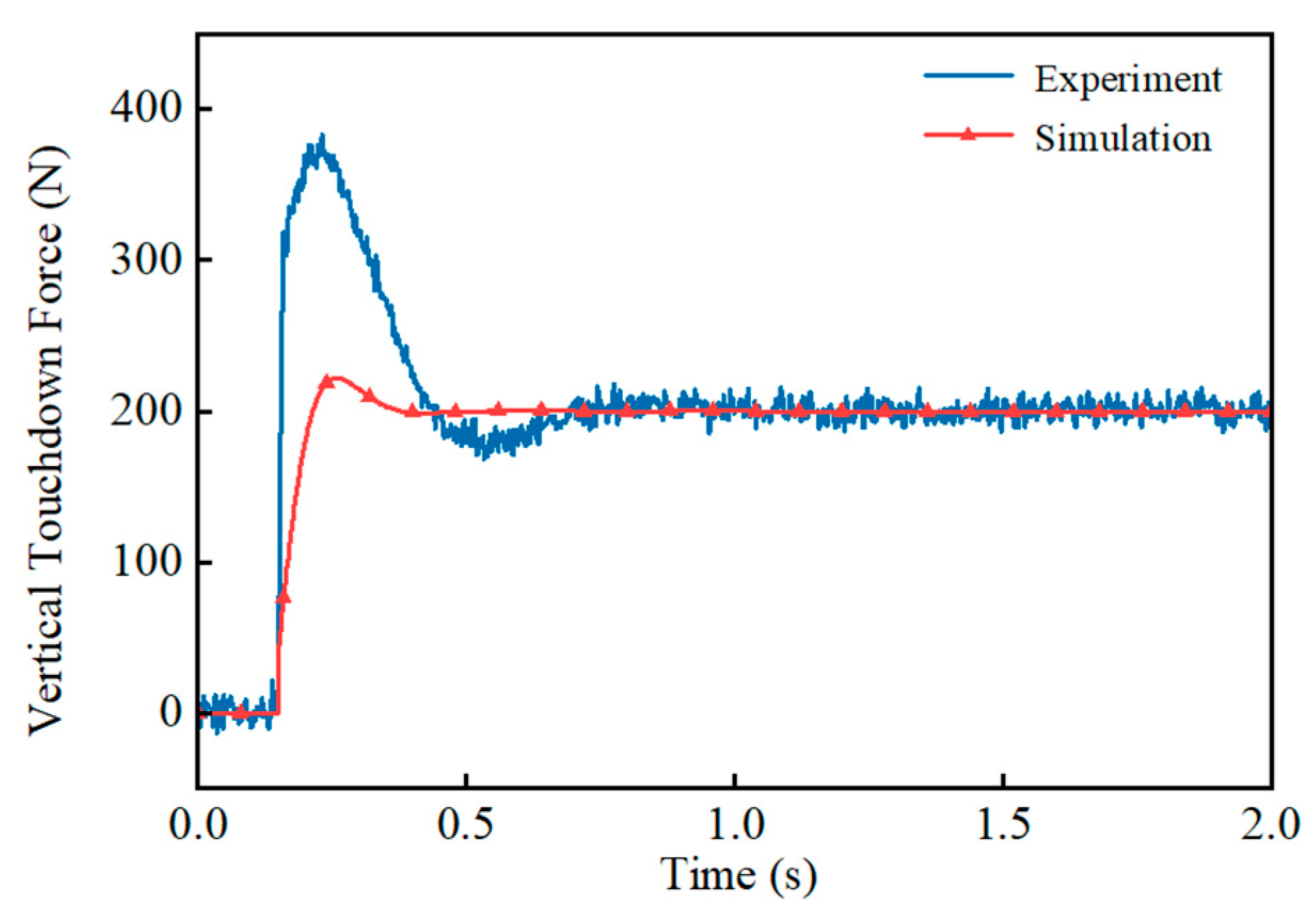
The force-based impedance control significantly reduces the touchdown force during the free-fall state of the single leg. Experimental results show that the maximum touchdown force is reduced to 45% without control, and there is no rebound phenomenon, which verifies the effectiveness of the method.

(3)

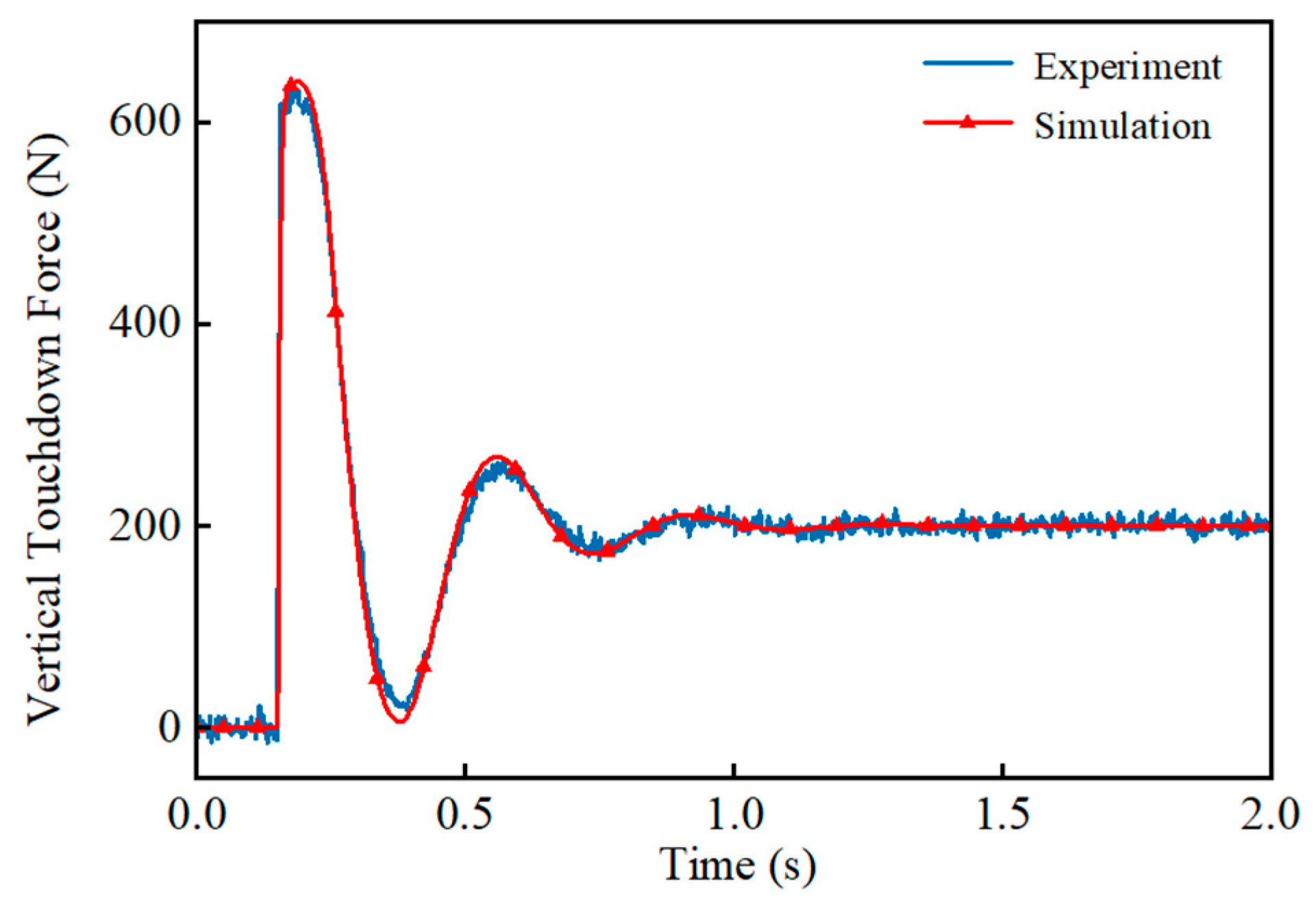
Admittance control indirectly controls the single-leg touchdown force by adjusting the end displacement to make it approach the desired value, thus effectively reducing the touchdown force. Experimental results show that this method reduces the maximum touchdown force to 61% of that without control, which proves its effectiveness and practicality.

References

1. Sheng, J.; Chen, Y.; Fang, X.; Zhang, W.; Song, R.; Zheng, Y.; Li, Y. Bio-inspired rhythmic locomotion for quadruped robots. IEEE Robot. Autom. Lett. 2022, 7, 6782–6789. [Google Scholar] [CrossRef]
2. Biswal, P.; Mohanty, P.K. Development of quadruped walking robots: A review. Ain Shams Eng. J. 2021, 12, 2017–2031. [Google Scholar] [CrossRef]
3. Tedeschi, F.; Carbone, G. Design issues for hexapod walking robots. Robotics 2014, 3, 181–206. [Google Scholar] [CrossRef]
4. Zhao, Y.; Chai, X.; Gao, F.; Qi, C. Obstacle avoidance and motion planning scheme for a hexapod robot Octopus-III. Robot. Auton. Syst. 2018, 103, 199–212. [Google Scholar] [CrossRef]
5. Sayyaadi, H.; Sharifi, M. Adaptive Impedance Control of UAVs Interacting with Environment Using a Robot Manipulator. In Proceedings of the Second RSI/ISM International Conference on Robotics and Mechatronics (ICRoM), Tehran, Iran, 15–17 October 2014; pp. 636–641. [Google Scholar]
6. Li, X.; He, J.; Feng, H.; Zhou, H.; Fu, Y. Research on Compliance Control for the Single Joint of a Hydraulic Legged Robot. In Proceedings of the IEEE International Conference on Robotics and Biomimetics (ROBIO), Kuala Lumpur, Malaysia, 12–15 December 2018; pp. 1720–1726. [Google Scholar]
7. Vukobratovic, M.; Surdilovic, D.; Ekalo, Y.; Katic, D. Dynamics and Robust Control of Robot-Environment Interaction; World Scientific: Singapore, 2009. [Google Scholar]
8. Ozawa, R.; Kobayashi, H.; Ishibashi, R. Adaptive impedance control of a variable stiffness actuator. Adv. Robot. 2015, 29, 273–286. [Google Scholar] [CrossRef]
9. Neville, H. Impedance control: An approach to manipulation: Part I-III. Trans. ASME J. Dyn. Syst. Meas. Control 1985, 107, 1. [Google Scholar]
10. Hogan, N. Impedance control: An approach to manipulation: Part II—Implementation. J. Dyn. Sys. Meas. Control. 1985, 107, 8–16. [Google Scholar] [CrossRef]
11. Boaventura, T.; Semini, C.; Buchli, J.; Frigerio, M.; Focchi, M.; Caldwell, D.G. Dynamic Torque Control of a Hydraulic Quadruped Robot. In Proceedings of the IEEE International Conference on Robotics and Automation, St Paul, MN, USA, 14–18 May 2012; pp. 1889–1894. [Google Scholar]
12. Grimminger, F.; Meduri, A.; Khadiv, M.; Viereck, J.; Wüthrich, M.; Naveau, M.; Berenz, V.; Heim, S.; Widmaier, F.; Flayols, T.; et al. An open torque-controlled modular robot architecture for legged locomotion research. IEEE Robot. Autom. Lett. 2020, 5, 3650–3657. [Google Scholar] [CrossRef]
13. Wang, S.; Chen, Z.; Li, J.; Wang, J.; Li, J.; Zhao, J. Flexible motion framework of the six wheel-legged robot: Experimental results. IEEE/ASME Trans. Mechatron. 2021, 27, 2246–2257. [Google Scholar] [CrossRef]
14. Hörger, M.; Kottege, N.; Bandyopadhyay, T.; Elfes, A.; Moghadam, P. Real-Time Stabilisation for Hexapod Robots. In Experimental Robotics: The 14th International Symposium on Experimental Robotics; Springer: Berlin/Heidelberg, Germany, 2015; pp. 729–744. [Google Scholar]
15. Ding, X.L.; Wang, Z.Y.; Rovetta, A. Typical gaits and motion analysis of a hexagonal symmetrical hexapod robot. Robot 2010, 32, 759–765. [Google Scholar]
16. Zhang, L.; Zha, F.; Guo, W.; Chen, C.; Sun, L.; Wang, P. Heavy-duty hexapod robot sideline tipping judgment and recovery. Robotica 2024, 42, 1403–1419. [Google Scholar] [CrossRef]
17. Roan, P.R.; Burmeister, A.; Rahimi, A.; Holz, K.; Hooper, D. Real-World Validation of Three Tipover Algorithms for Mobile Robot. In Proceedings of the IEEE International Conference on Robotics and Automation, Anchorage, AK, USA, 3–8 May 2010; pp. 4431–4436. [Google Scholar]
18. Hutter, M.; Gehring, C.; Jud, D.; Lauber, A.; Bellicoso, C.D.; Tsounis, V.; Hwangbo, J.; Bodie, K.; Fankhauser, P.; Bloesch, M.; et al. Anymal-a Highly Mobile and Dynamic Quadrupedal Robot. In Proceedings of the International Conference on Intelligent Robots and Systems (IROS), Daejeon, Republic of Korea, 9–14 October 2016; pp. 38–44. [Google Scholar]
19. Sokolov, A.; Xirouchakis, P. Kinematics of a 3-DOF parallel manipulator with an RPS joint structure. Robotica 2005, 23, 207–217. [Google Scholar] [CrossRef]
20. Hervé, J.M. The Lie group of rigid body displacements, a fundamental tool for mechanism design. Mech. Mach. Theory 1999, 34, 719–730. [Google Scholar] [CrossRef]
21. Song, S.M.; Waldron, K.J. Machines that Walk: The Adaptive Suspension Vehicle; MIT Press: Cambridge, MA, USA, 1989. [Google Scholar]
22. Xu, F.X.; Liu, X.H.; Chen, W.; Zhou, C.; Cao, B.W. Improving handling stability performance of four-wheel steering vehicle based on the H2/H∞ robust control. Appl. Sci. 2019, 9, 857. [Google Scholar] [CrossRef]
23. Ghasemi, M.; Deriche, M.; Trojovský, P.; Mansor, Z.; Zare, M.; Trojovská, E.; Abualigah, L.; Ezugwu, A.E.; kadkhoda Mohammadi, S. An efficient bio-inspired algorithm based on humpback whale migration for constrained engineering optimization. Results Eng. 2025, 25, 104215. [Google Scholar] [CrossRef]
24. Zhu, Y.; Liu, C.; Yuan, P.; Li, D. Active impedance control based adaptive locomotion for a bionic hexapod robot. J. Field Robot. 2025, 42, 327–345. [Google Scholar] [CrossRef]
Figure 1. Single-leg construction diagram.
Applsci 15 05312 g001
Figure 2. Diagram of the D–H coordinate system of the main kinematic chain.
Applsci 15 05312 g002
Figure 3. Schematic diagram of stabilization cone.
Applsci 15 05312 g003
Figure 4. The flowchart diagram of the finite state machine.
Applsci 15 05312 g004
Figure 5. Schematic diagram of the quadrupedal gait stepping-out scenario.
Applsci 15 05312 g005
Figure 6. Figure of the quadrupedal support gait.
Applsci 15 05312 g006
Figure 7. Schematic diagram of the tripod gait stepping-out scenarios.
Applsci 15 05312 g007
Figure 8. Figure of the tripod gait.
Applsci 15 05312 g008
Figure 9. The schematic diagram of admittance control.
Applsci 15 05312 g009
Figure 10. Curve diagram of the fitness value.
Applsci 15 05312 g010
Figure 11. Variation curves of touchdown force and position with inertia parameters: (a) curve of touchdown force; (b) curve of position.
Applsci 15 05312 g011
Figure 12. Variation curves of touchdown force and position with damping parameters: (a) curve of touchdown force; (b) curve of position.
Applsci 15 05312 g012
Figure 13. Variation curves of touchdown force and position with stiffness parameters: (a) curve of touchdown force; (b) curve of position.
Applsci 15 05312 g013
Figure 14. Dynamic response diagrams of impedance parameters optimized by two methods: (a) curve of touchdown force; (b) curve of position.
Applsci 15 05312 g014
Figure 15. Equivalent schematic of pit-probing simulation.
Applsci 15 05312 g015
Figure 16. Simulation of touchdown force-time at the end of the pit-probing.
Applsci 15 05312 g016
Figure 17. Force-based impedance control schematic.
Applsci 15 05312 g017
Figure 18. Equivalent schematic for free-fall simulation.
Applsci 15 05312 g018
Figure 19. Force–time simulation plot.
Applsci 15 05312 g019
Figure 20. Acceleration–time simulation plot.
Applsci 15 05312 g020
Figure 21. Experimental framework diagram.
Applsci 15 05312 g021
Figure 22. Single leg prototype diagram.
Applsci 15 05312 g022
Figure 23. Pure positional control of leg movement processes.
Applsci 15 05312 g023
Figure 24. No impedance force at the foot-end of the falling body in the vertical direction.
Applsci 15 05312 g024
Figure 25. Single-leg free-fall motion process without impedance control.
Applsci 15 05312 g025
Figure 26. Impedance force at the foot-end of the falling body in the vertical direction.
Applsci 15 05312 g026
Figure 27. Single-leg pit-probing motion process.
Applsci 15 05312 g027
Figure 28. No admittance control pit-probing vertical foot-end force.
Applsci 15 05312 g028
Figure 29. Admittance control pit-probing vertical foot-end force.
Applsci 15 05312 g029