Analysis of Stochastic Properties of MEMS Accelerometers and Gyroscopes Used in the Miniature Flight Data Recorder

Featured Application

The potential use of presented methods for the selection of appropriate sensors for measurement systems and synthesis of measurement algorithms. The establishment of the application possibilities, limitations, and appropriate operating conditions of existing measurement systems.

Abstract

MEMS (micro-electro-mechanical system) gyroscopes and accelerometers are used in several applications. They are very popular due to their small size, low price, and accessibility. The design of MEMS accelerometers enables the measurement of vibrations, with frequencies from tenths of hertz to even 1 kHz. MEMS gyroscopes can be applied to measure angular rates, and indirectly also angular oscillations with frequencies similar to accelerometers. Despite significant stochastic errors, MEMS sensors are used not only in popular domestic appliances (e.g., smartphones) but also in safety-critical units, such as aeronautical attitude and heading reference systems (AHRSs). In engineering, methods of stochastic properties analysis are important tools for sensor selection, verification, and the design of measurement algorithms. In this article, three methods used for the analysis of stochastic properties of sensors are presented and comparative analyses are shown. The applied measurement frequencies (1 kHz) were much higher than those typically found in MEMS sensor applications. Additionally, an exemplary analysis of temperature drift frequency, as well as the possibility for the synthesis of complementary filter parameters with the use of the described methods, is shown. Assessment of the stochastic properties of MEMS accelerometers and gyroscopes was performed under both constant and variable temperature conditions (during warm-up after switching on) with the use of classic methods, such as power spectral density (PSD) and Allan variance (AV), as well as the less known but very promising generalized method of wavelet moments (GMWM).

1. Introduction

Measurement systems are essential elements of modern aircraft equipment. Basic values measured on board aircraft are air data (airspeeds—indicated airspeed and true airspeed, altitude, rate of climb), inertial data (angular rates, accelerations, attitude—pitch and roll angle, heading), and navigation data. Inertial data are used not only during the flight control process, but they are significant in research processes, such as the mathematical model identification process, or vibration analyses. Inertial data are based on measurements from gyroscopes and accelerometers. Their technology has a significant influence on measurement system properties. MEMS gyroscopes and MEMS accelerometers are commonly used in aeronautical applications. Characteristic examples of such applications are presented in the works [1,2,3,4,5]. Because of their small size, they are the only possible choice for small UAVs [6,7]. Due to their low cost, they are popular in General Aviation planes for control and data recording systems [8,9,10].

Vibrations and oscillations occurring on board aircraft are characterized by a very wide range of possible frequencies. Compressor blades can oscillate with a frequency of several thousand hertz [11]. In the case of piston engines, vibrations with frequencies reaching hundreds of hertz should be expected [12]. The aircraft oscillation frequency, characteristic of short-period motion, is counted in single hertz for small sport aircraft [13] and in tenths of hertz for large structures [13,14]. The period of oscillation in phugoid motion reaches even hundreds of seconds [14]. The same applies to the amplitudes of the co-occurring phenomena, which, depending on the class of the phenomenon and the phase of flight, may be close to measurement noise, and in another extreme case—reach beyond the operating range of the measuring equipment, even leading to its destruction.

For a proper choice of measurement system elements, it is necessary to take into consideration several aspects, such as, for instance, environmental conditions or measurement system properties. First, it is necessary to analyze the properties of the measured signals (typical frequencies appearing in the system, as well as signal bands). With the knowledge of signal properties, sensors can be selected. The properties of the sensors are of great significance. They also determine the behavior of calculated signals. Very important data registered on board aircraft are attitude angles. They are calculated from angular rates and corrected by accelerations. As mentioned, the properties of attitude angles depend on angular rate and acceleration sensor properties, as well as the data estimation algorithm.

When analyzing the applicability of sensors, the nominal operating range of the system (measurement range), acceptable environmental conditions, and errors occurring in static and dynamic conditions are usually taken into account. Measurement frequency is determined by the purpose of measurements and data collection, as well as the task and kind of aircraft. Usually, for control, it is necessary to measure accelerations and angular rates with frequencies from 10 Hz up to 400 Hz. For other purposes, the desired frequencies are much higher. For sensor selection, it is vital to verify MEMS stochastic properties. The properties of sensors strongly influence the calculated attitude. 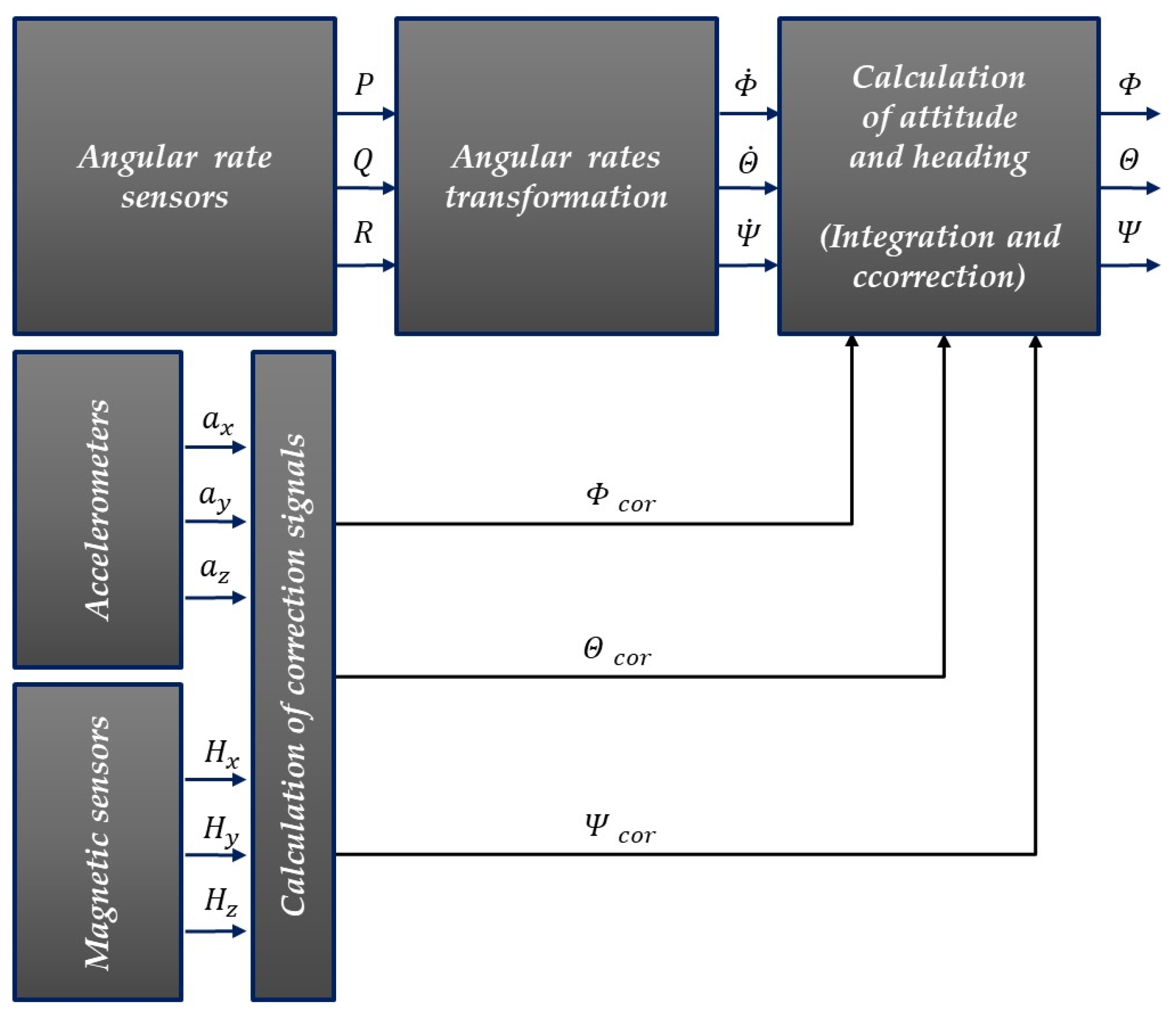Figure 1 shows a general scheme of the attitude and heading reference system (AHRS).

The AHRS system provides attitude angles and headings. Angular rate sensors measure angular rates P, Q, and R, in the body frame. To calculate attitude and heading, angular rates are transformed from the body frame to the earth frame. Next, angular rates $\dot{\Phi }$, $\dot{\Theta }$, and $\dot{\Psi }$ in the earth frame are integrated and corrected. For correction, two algorithms are usually used. The first one is the Kalman filter [15], and the second one is the complementary filter [16], also used in several other solutions [15,17,18,19,20]. The Kalman filter minimizes the estimated value variance error, which makes it highly popular. However, its disadvantage is its computational complexity, which increases computational costs [21]. For this reason, it is the complementary filter that is applied in some solutions for the calculation of attitude and heading angles. From the angular rate, an angle can be easily calculated:

$${\phi }_G={\displaystyle \int }a{s}_{g}dt$$

(1)

where

• $a{s}_g$—angular speed from gyroscopes;
• ${\phi }_G$—angle calculated from gyroscopes.

Another way to estimate the angle is by calculating it from accelerometer data, e.g.,:

$${\phi }_{acc}={\tan }^{-1}\frac{a_y}{a_z}$$

(2)

where

• $a_y,a_z$—horizontal and vertical acceleration from accelerometers.

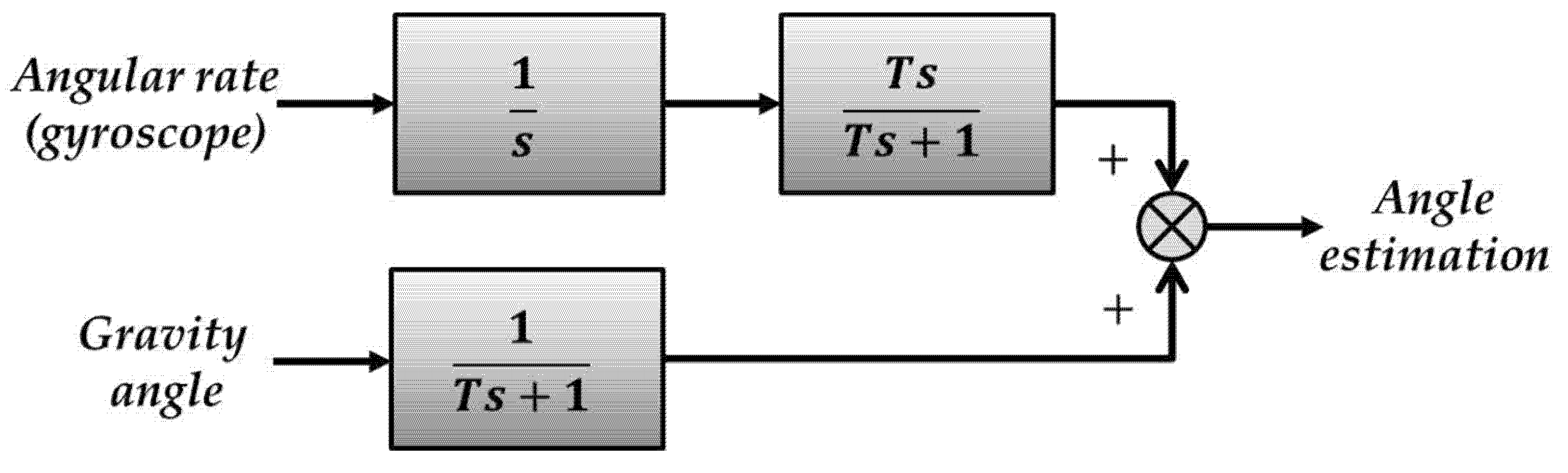
Angles calculated from gyroscope data are burdened with low-frequency errors (drift). Angles calculated from accelerometers are burdened with noises, which are high-frequency errors. For the minimalization of errors, both sensors should be used. Figure 2 presents a scheme with a complementary filter.

Gyroscopic data, after integration, are filtered by a high-pass filter, which eliminates low-frequency errors. A low-pass filter allows the elimination of noises from accelerometers. A sum of both filtered signals is a satisfactory approximation of the real value. Time constant T is the designing parameter. For the proper choice of the T parameter, information about the sensors’ stochastic parameters is essential.

The presented analysis shows that quantitative analysis of the stochastic properties of accelerometers and gyroscopes is a significant element of the measurement system design. The aim of this article is to compare methods used for the analysis of stochastic properties, and to present possibilities of application in engineering. The comparative analysis of stochastic properties is performed with the PSD method, the Allan variance method (the application of these two methods is determined by appropriate standards [22,23]), and the generalized method of wavelet moments [24,25,26]. The GMWM is a relatively new, and hence less known, but potentially the most interesting method. Studies in which the GMWM method is used for the analysis of stochastic errors in AHRS systems [27] and inertial navigation units [28], including smartphones [29], are scarce. They are also relatively new, as the method was made public in 2013 [24]. The GMWM method is usually compared with the AV method [30], or the GMWM alone is used to determine the stochastic errors [28]. The analyses in papers [27,28,29,30] focus on sampling frequency from 10 to max 200 Hz.

This article presents the stochastic properties of MEMS sensors, especially for high sampling frequency (1 kHz). Analyses of the stochastic properties of MEMS sensors with such a high frequency can rarely be found in research papers. With high sampling frequency, it is possible to realize an AHRS synthesis that enables high precision control of high-maneuverability objects. With the oversampling of sensor data, it is also possible to apply additional methods of signal processing due to which a lower frequency AHRS can be fed with more accurate and reliable input data. Application of high-sampling-frequency accelerometers and gyroscopes enables precise analysis of flight parameters, including, e.g., short-period oscillations, with frequencies as high as hundreds of Hz, of mini-UAVs [31,32].

The properties relating to the construction of MEMS sensors, their dimensions, and their weight are a separate problem linked with the technical possibilities of their application. In the data sheets of most MEMS-class products, the potential user will find information about the sensitivity of the measurement system, noise level (mean square value, power spectral density), and natural oscillator frequencies. The parameters of the output filters are usually configurable (programmable). The programmable parameters are usually the sampling rates, gain factors, and offsets [33,34]. In the case of some measurement systems, manufacturers also provide a calibration certificate, containing programmed values of gains and offsets and the results of tests performed for a specific unit.

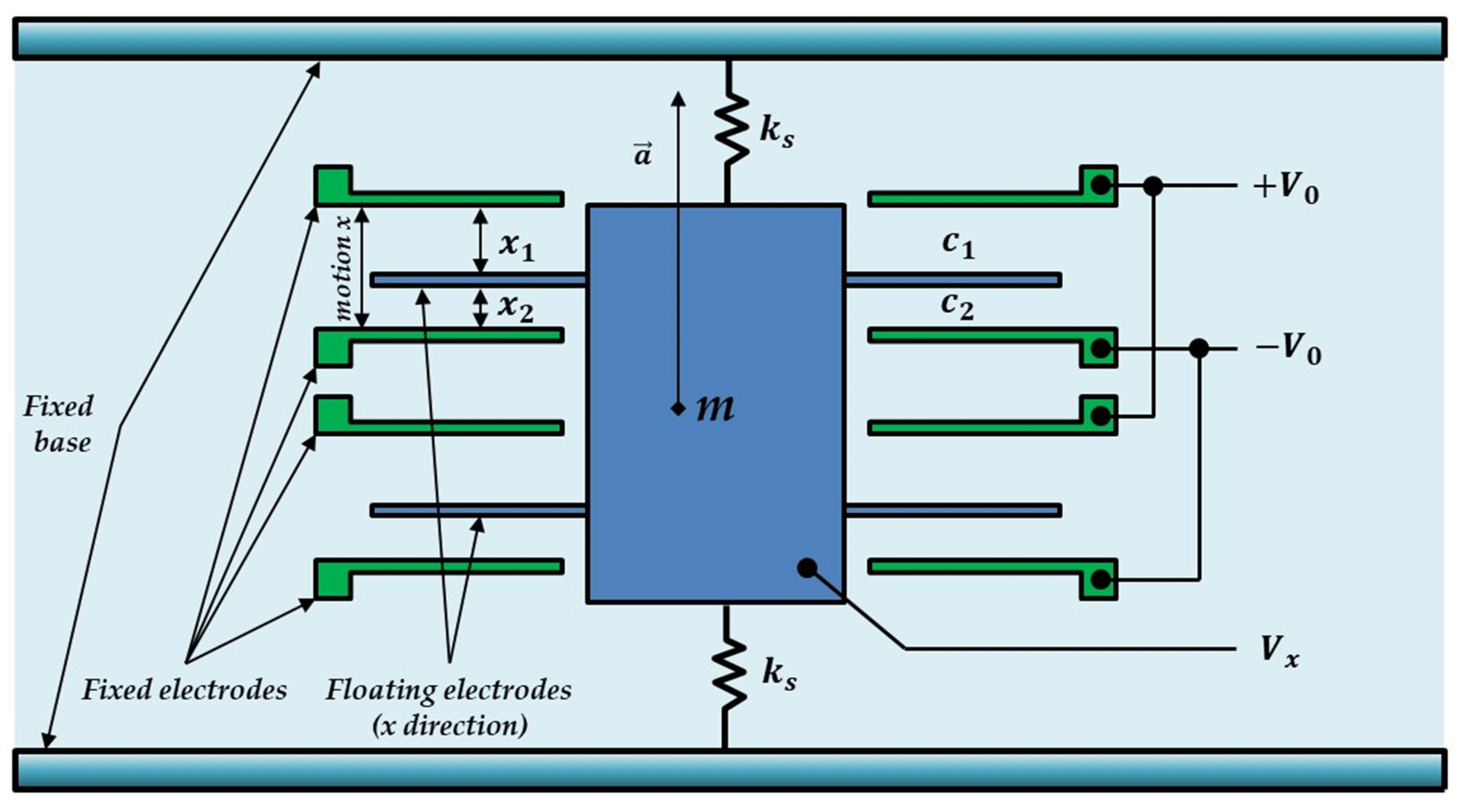
The mass sample contained in a MEMS accelerometer is typically a few tenths of a microgram (Figure 3). The smallest detectable capacity change is currently several attofarads, and the distances between the plates are of the order of one micrometer [35]. The operating frequency of the oscillator must be several orders of magnitude higher than the desired acceleration measurement frequency since the capacitance reading process using the demodulator requires a large number of cycles to determine the output value. The measurement noise resulting from this process is inversely proportional to the root of frequency and can be modeled as quantization noise. For static measurements near zero, the value of this noise may exceed the measured acceleration. In typical MEMS accelerometers, there are at least two other sources of noise, which are the mechanical vibrations of the microstructure and interference introduced by the output circuits of the amplifier and low-pass filter. The causes of noise in MEMS gyroscopes are analogous [36,37]. Stochastic processes caused by these phenomena, among others, are discussed in detail in the following sections.

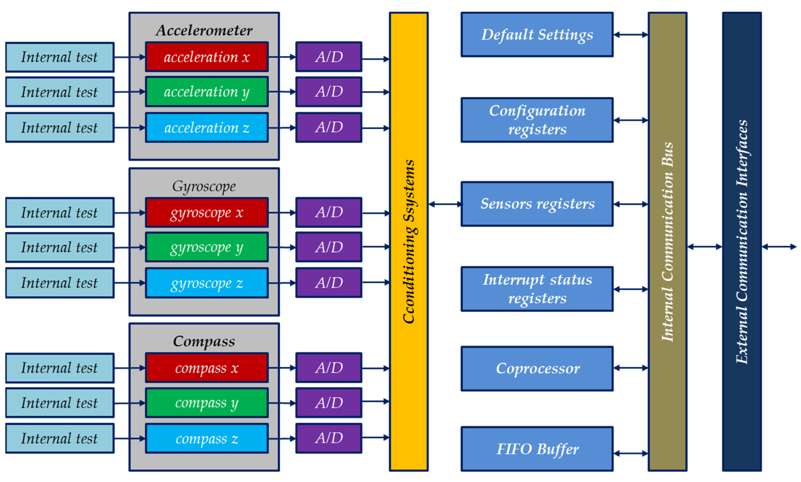
To obtain high precision of measurements, accelerometers and gyroscopes should be calibrated. Calibration errors resulting from inaccuracies in the manufacturing and assembly process of the device are minimized and temperature compensation is performed. A simplified block diagram of a three-axis accelerometer integrated with a gyroscope and magnetometer is shown in Figure 4.

This paper will analyze in detail the measurement properties of 3D accelerometer and 3D gyroscope assemblies produced using MEMS technology. The main purpose of the presented analysis is to demonstrate the validity of the use of selected IMUs (inertial measurement units) on board small aircraft and UAVs (unmanned aerial vehicles). In miniature UAVs, high sampling frequencies of angular rates and accelerations are desired. This is important for attitude and heading calculation in AHRS, but such high sampling frequencies are especially important in flight recorders used for research purposes. The registered data can, for example, be used for the identification of aircraft characteristic frequencies. The stochastic analysis of MEMS inertial sensors in advanced IMUs in this article presents reliable information about the IMU properties not only for this particular system but can also be helpful in the synthesis of complementary filter parameters used in different AHRSs. The comparative analysis in this paper was performed with the use of three methods for all six sensors; temperature change was also considered. The presented approach to IMU research, which is an element of a miniature flight parameter recording system, has an original character, intended to lead to non-obvious subsequent research tasks.

2. Power Spectral Density of Selected Disturbances

The process of quantization of the signal causes a measurement error that cannot be removed. Assuming an even distribution of the probability of the occurrence of a value in the quantization interval q, the dependence on the covariance of the quantization noise is obtained from (3) [22]:

$${\sigma }^2=\frac{q^2}{12}$$

(3)

The spectral density is determined by the relationship (4) [22,39,40]:

$$S\left(f\right)=\{\begin{array}{c}\frac{4Q^2}{{\tau }_0}{\sin }^2\left(\pi f{\tau }_0\right)\\ \begin{array}{cc}{\left(2\pi f\right)}^2{\tau }_0{Q}^2& dla f<\frac{1}{2{\tau }_0}\end{array}\\ \end{array}$$

(4)

where ${\tau }_0$ is the sampling period and $Q$ is the quantization noise coefficient (factor).

Angle random walk (ARW) gyroscope white noise or velocity random walk (VRW) accelerometer white noise can be represented as power spectral density:

$$S\left(f\right)=N^2$$

(5)

where $N$ is the noise coefficient $\left(°/\sqrt{s}\right)$ from the gyroscope and $\left(\left(\frac{m}{s}\right)/\sqrt{s}\right)$ from the accelerometer.

Power spectral density (PSD) in the case of drift of inertial sensors is determined by the following formula:

$$S\left(f\right)=\{\begin{array}{r}{\left(\frac{B}{2\pi }\right)}^2\frac{1}{f}, f\le f_c\\ 0, f>f_c\end{array}$$

(6)

where $B$ is the drift coefficient and $f_c$ is the crossover frequency.

The power spectral density of the Brownian noise (red noise) of the gyroscope (rate random walk—RRW) is represented by the formula

$$S\left(f\right)={\left(\frac{K}{2\pi }\right)}^2\frac{1}{f^2}$$

(7)

where $K$ is the RRW/RW noise coefficient.

The PSD of the accelerometer’s Brownian noise (random walk—RW) is similarly described. The power spectral density of the trend function, which expresses a uniform change in the signal value, is determined from the formula

$$S\left(f\right)=\frac{R^2}{{\left(2\pi f\right)}^3}$$

(8)

where $R$ is the trend coefficient.

Harmonic interference may occur when equipment is powered from the 115 VAC/400 Hz onboard network or during laboratory testing of equipment powered by 230 VAC/50 Hz.

The power spectral density of this type of interference is expressed by the following formula:

$$S\left(f\right)=\frac{1}{2}A\left[\delta \left(f-f_0\right)+\delta \left(f+f_0\right)\right]$$

(9)

where $A$—the amplitude of the disturbance, $f_0$—the frequency of the jamming signal, and $\delta$—the Dirac delta.

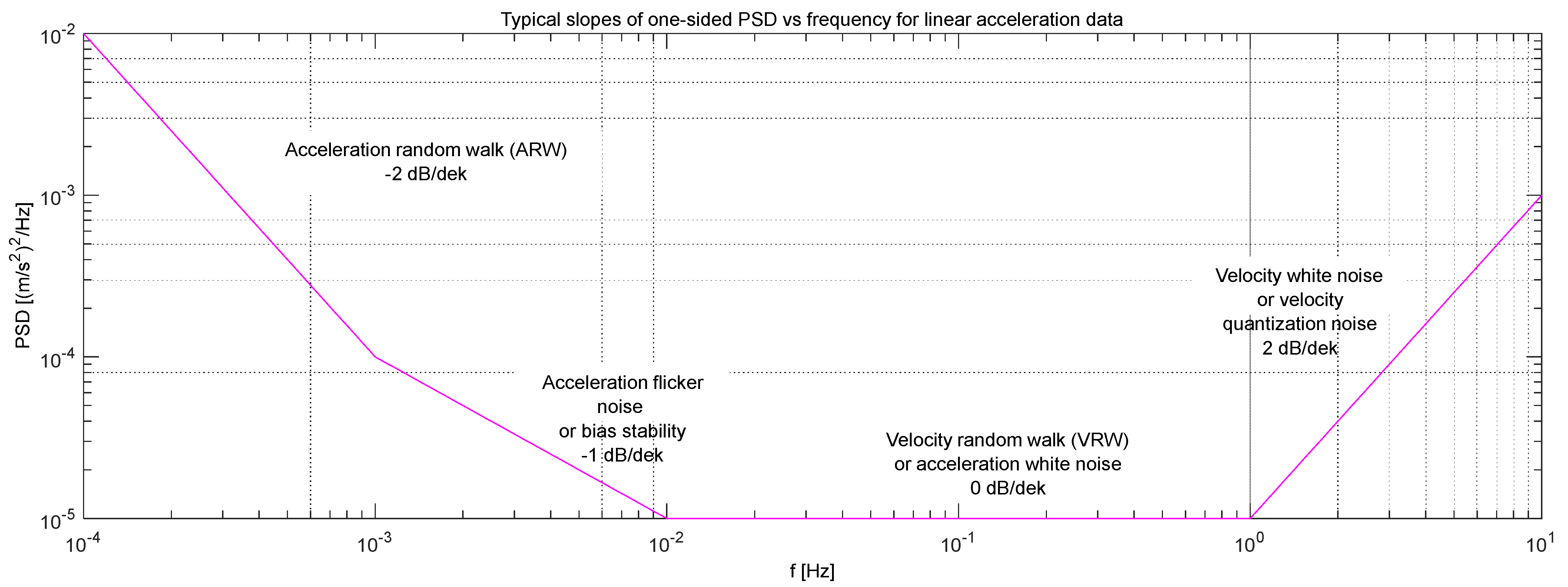
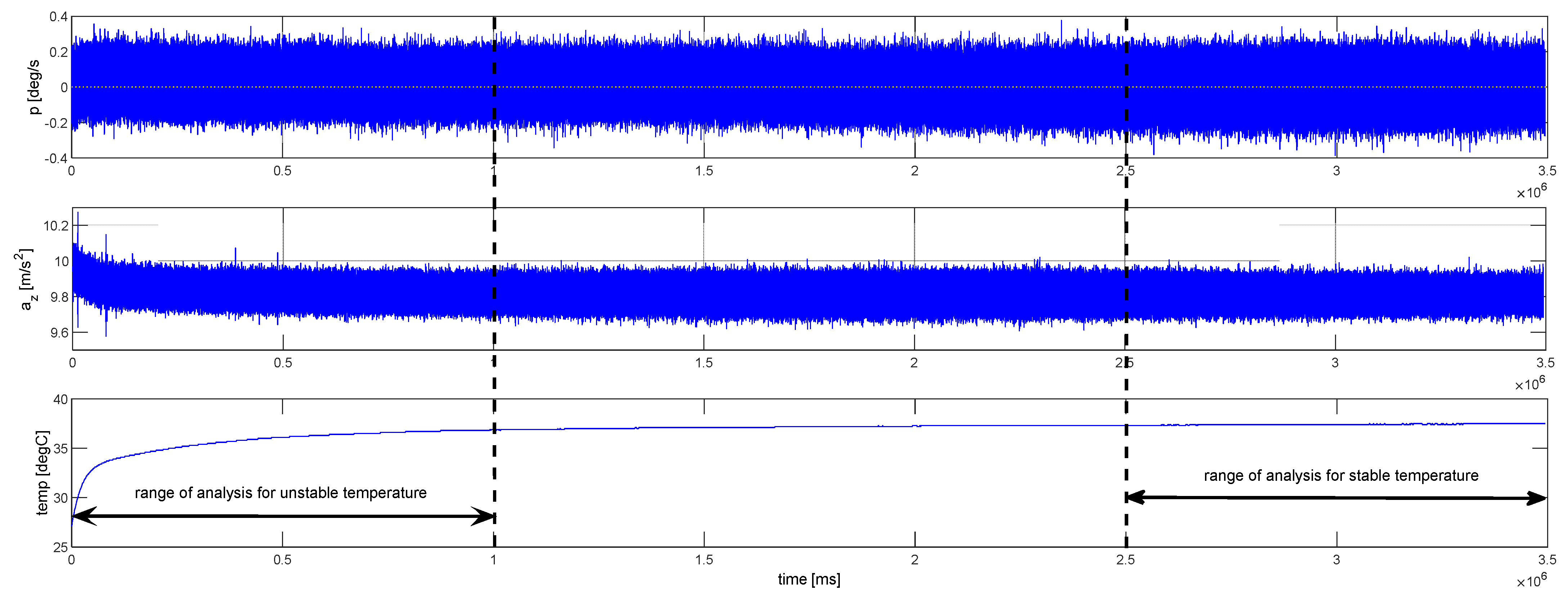
The hypothetical course of the PSD characteristic for the inertial sensor is presented in Figure 5 [23]. In practice, in order to determine this characteristic, it is necessary to register a set of test data in static conditions, including at least 10⁶ samples [41]. The test data should be corrected for the initial offset value [23]. 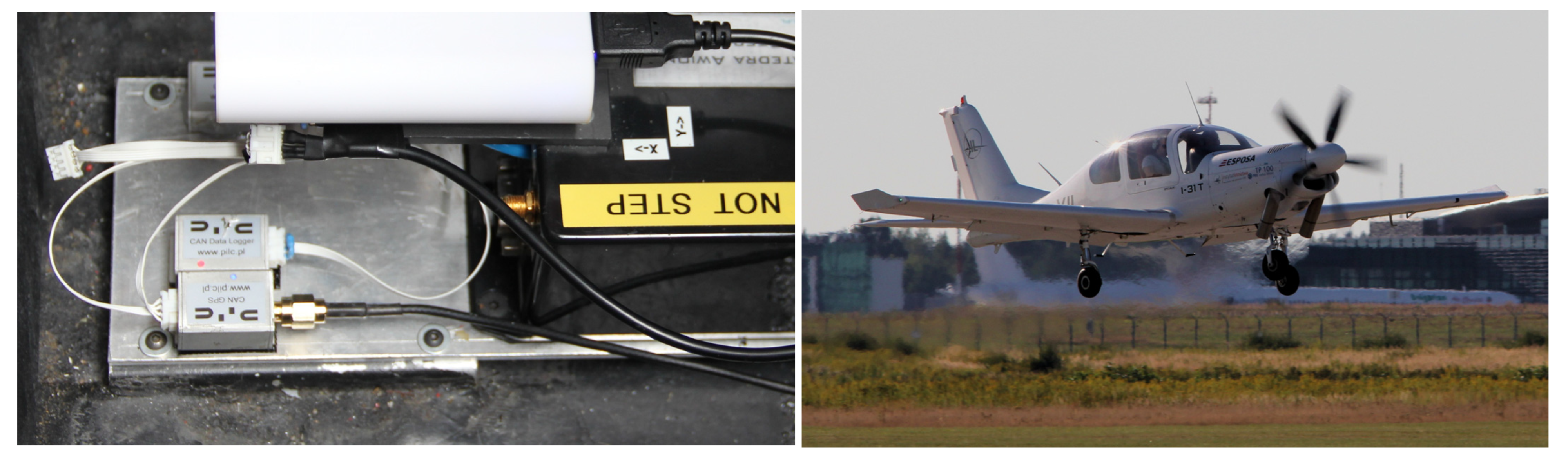Figure 6 shows time courses of roll rate (p), longitudinal acceleration (a_x), and sensor module temperature (T) obtained from the PCIM-01 IMU module [42] cooperating with the PRP-W2 recorder (Figure 7). The signal sampling frequency was 1 kHz. 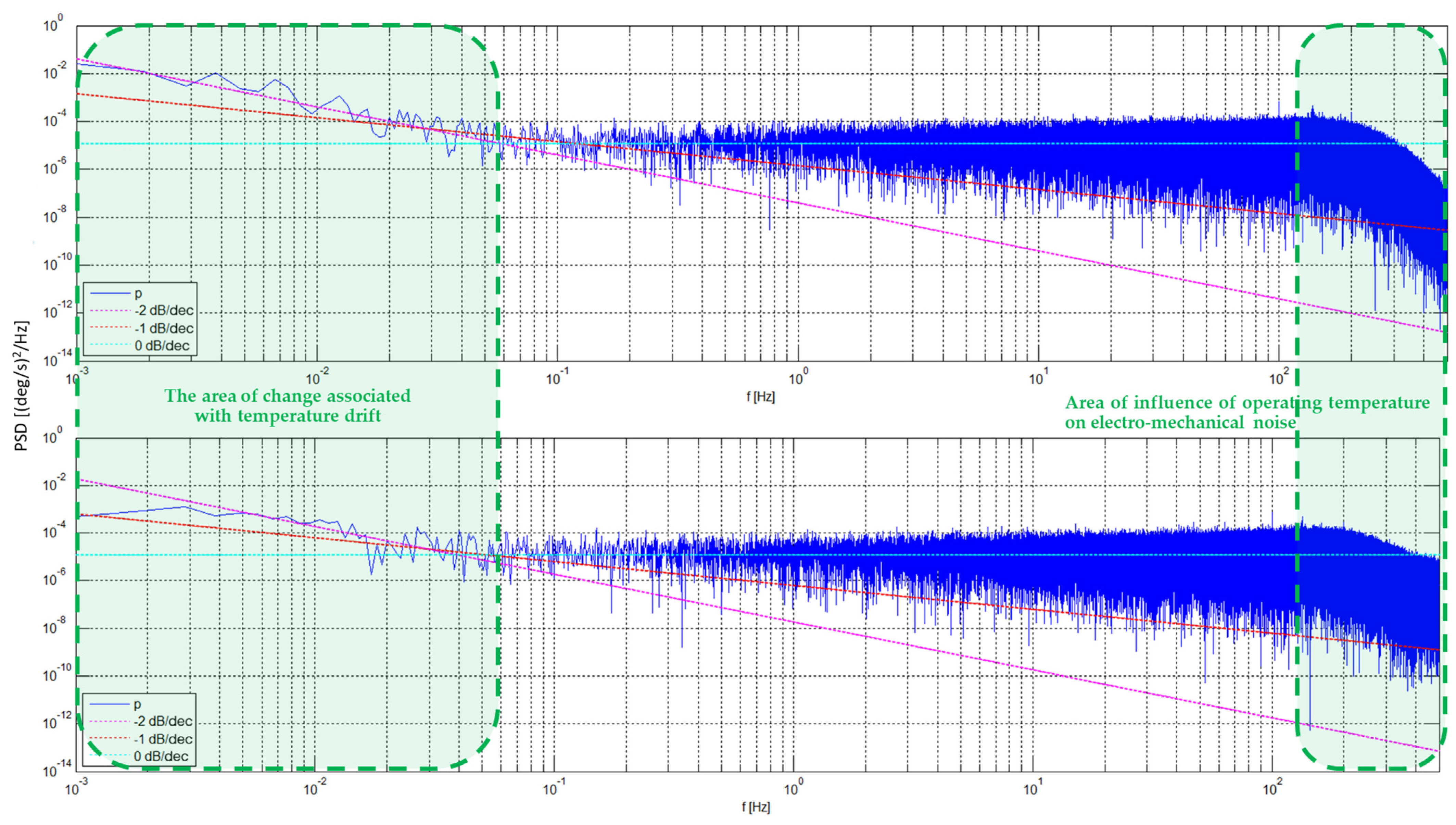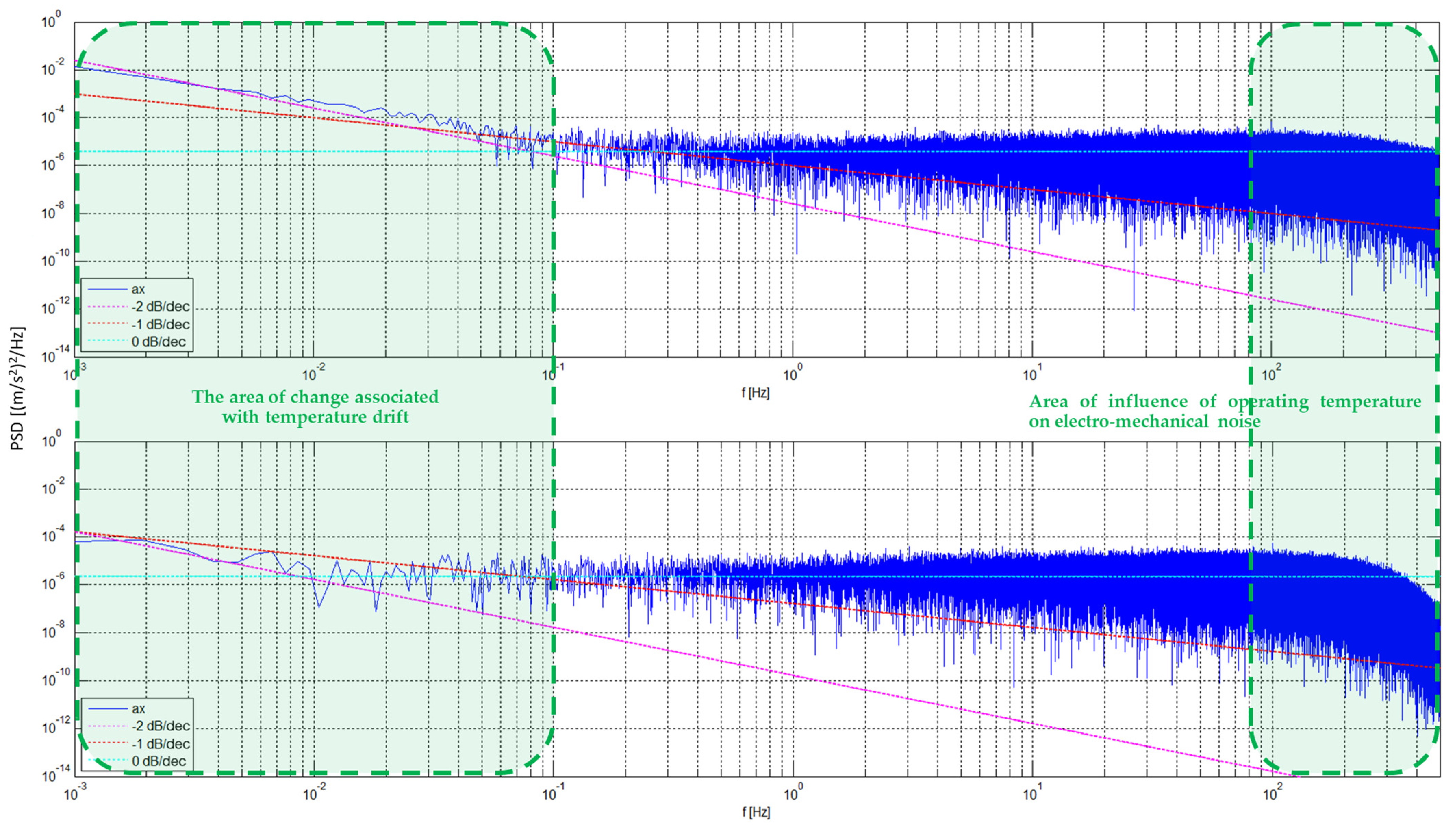Figure 8 shows the power spectral density for two data sets of roll rate selected from one test, which lasted about an hour in total. For comparative purposes, the PSD of the signal was generated for two cases. First, PSD was generated for 10⁶ samples recorded just after switching on the device. In this case, the temperature rose from 27.1 °C to 36 °C. A second series of 10⁶ samples began to be recorded 2490 s after switching on, when the temperature of the IMU assembly (Figure 6) reached a relatively constant temperature (in practice it changed between 2490 and 3490 s in the range of 37.3–37.5 °C). Figure 6 shows the temperature course of the sensor during the entire experiment, as well as the time course of the angular velocity p around the x-axis.

The recorded angular velocity oscillated during the static test in the range of −0.4–0.4 deg/s. The amplitude of the oscillations increased slightly with the temperature increment. After reaching a constant temperature, the mean signal value stabilized and approached zero. These phenomena can also be observed in the PSD charts in Figure 8. The gyroscope drift due to temperature change is approximated by a line with a slope of −2 dB in the frequency range 0.001–0.09 Hz (Figure 8, upper subplot). For a stabilized operating temperature of the sensor, this drift is in fact very difficult to determine via the power spectral density plot. However, in the high-frequency range, the phenomenon of increasing noise is observed, which is the result of the influence of higher temperature on the electrical and mechanical vibrations in MEMS systems [43,44]. This change is clearly observed for the tested gyroscopes in Figure 8 for the frequency range of 300–500 Hz. The noise level increases, but in practice, due to the programmable low-pass filter built into the system, it does not affect the quality of the measurements.

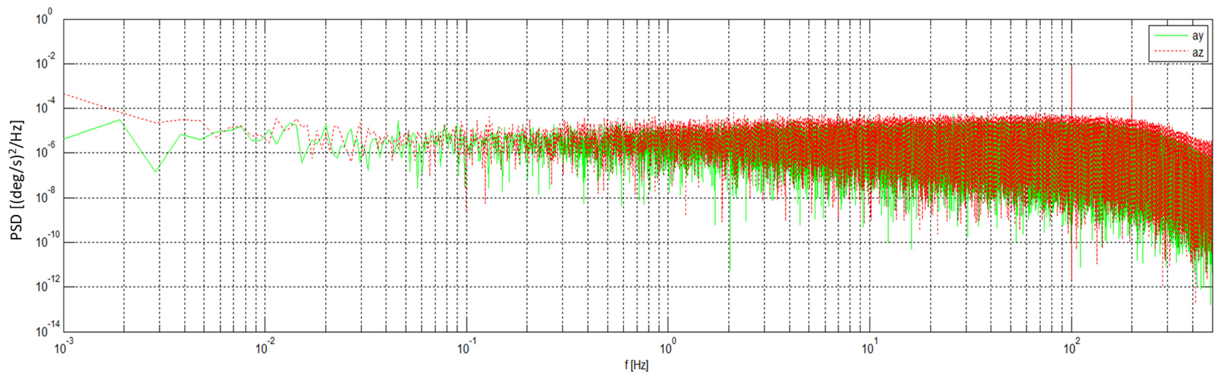
In the tested system, the cut-off frequency was set to the maximum value, which is 256 Hz. Figure 9 shows the collective PSD characteristics for the gyroscopes installed in the pitch and yaw channel, obtained on the basis of data recorded during the same experiment. These relationships are consistent with the results obtained for the angular velocity of the roll.

Figure 10 and Figure 11 show the one-sided PSD determined for the set of accelerometers of the IMU system, which is one of the measurement modules of the PRP-W2 recording system. The measurement data for accelerometers and gyroscopes are from the same measurement session (Figure 6, Figure 7, Figure 8, Figure 9, Figure 10 and Figure 11). In the case of PSD plots obtained for accelerometers, similarly to gyroscopes, the phenomenon of temperature drift in the frequency range from 10⁻³ to 10⁻¹ Hz can be observed (Figure 10). Nevertheless, the influence of the increased operating temperature of the system on the noise level in the highest frequency range has a completely different character. According to the information in the literature [45], an increase in the temperature of the sensor shifts the resonance frequency of the electromechanical vibrations of the MEMS accelerometer towards lower frequencies. However, this fact can hardly be interpreted unambiguously on the basis of the analysis of the PSD diagram obtained (Figure 10 and Figure 11). As in the case of the tested gyroscopes, the level of noise in this range has no practical importance. In the analyzed accelerometer system, the low-pass filter cut-off frequency was set to a maximum value of 260 Hz.

The range of the analysis and noise comparison of individual gyroscopes and accelerometers was limited to two intervals. The first interval was when the sensors were warming up, and the second was when sensors reached a constant operating temperature (time intervals are marked in Figure 6). The values of the determined noise coefficients are presented in

Table 1. Gyroscope noise coefficients determined by the following methods: PSD, AV, and GMWM.

Noise Coefficients of Gyroscopes	Angular Velocity P			Angular Velocity Q			Angular Velocity R
	PSD Method	AV Method	GMWM Method	PSD Method	AV Method	GMWM Method	PSD Method	AV Method	GMWM Method
Measurements for gyroscopes during IMU self-heating
N (ARW) $[\mathrm{deg}/\sqrt{\mathrm{s}}$]	0.00350	0.00305	0.00308	0.00400	0.00324	0.00328	0.00400	0.00337	0.00340
B (BI) [deg/s]	0.00200	0.00180	0.00185	0.00300	0.00212	0.00216	0.00250	0.00182	0.00182
K (RRW) $\mathrm{deg}/\left(\mathrm{s}\sqrt{\mathrm{s}}\right)$]	0.00085	-	0.0006 *	0.00005	0.00140	0.00140	0.00040	0.00107 *	0.0008 *
Measurements for gyroscopes at a fixed temperature of the IMU
N (ARW) $[\mathrm{deg}/\sqrt{\mathrm{s}}$]	0.00400	0.00311	0.00316	0.00400	0.00330	0.00332	0.00400	0.00344	0.00346
B (BI) [deg/s]	0.00100	0.00047	0.00046	0.00050	0.00091	0.00091	0.00250	0.00112	0.00112
K (RRW) $[\mathrm{deg}/\left(\mathrm{s}\sqrt{\mathrm{s}}\right)$]	0.00015 *	0.00010	0.00008	0.00030 *	0.00044 *	0.00015 *	0.00070 *	0.00022	0.00025

* Approximate values of coefficients obtained for sections whose inclination in practice did not reach the full values resulting from theoretical models.

and

Table 2. Accelerometer noise coefficients determined by the following methods: PSD, AV, and GMWM.

Accelerometer Noise Coefficients	ax			ay			az
	PSD Method	AV Method	GMWM Method	PSD Method	AV Method	GMWM Method	PSD Method	AV Method	GMWM Method
Measurements for accelerometers during IMU self-heating
N (VRW) $\left[\right(\mathrm{m}/{\mathrm{s}}^2)/\sqrt{\mathrm{s}}$]	0.00180	0.00128	0.00140	0.00160	0.00125	0.00140	0.00250	0.00169	0.00187
B (BI) [(m/s2)/s]	0.00021	0.00074	0.00029	0.00150	0.00057	0.00034	0.00500	0.00140	0.00031
K (RW) $[\left(\mathrm{m}/{\mathrm{s}}^2\right)/\left(\mathrm{s}\sqrt{\mathrm{s}}\right)$]	0.00080	0.00025	0.00025	0.00050	0.00018	0.00019	0.00490	0.00122	0.00125
Measurements for accelerometers at a fixed temperature of the IMU
N (VRW) $\left[\right(\mathrm{m}/{\mathrm{s}}^2)/\sqrt{\mathrm{s}}$]	0.00150	0.00124	0.00141	0.00150	0.00123	0.00141	0.00200	0.00170	0.00184
B (BI) [(m/s2)/s]	0.00100	0.00029	0.00029	0.00060 *	0.00017	0.00018	0.00080 *	0.00031	0.00031
K (RW) $[\left(\mathrm{m}/{\mathrm{s}}^2\right)/\left(\mathrm{s}\sqrt{\mathrm{s}}\right)$]	0.00008 *	-	0.00004 *	0.00004 *	0.00003 *	0.00002 *	0.00010 *	0.00006	0.00006

* Approximate values of coefficients obtained for sections whose inclination in practice did not reach the full values resulting from theoretical models.

and compared with the results obtained with the Allan variance method.

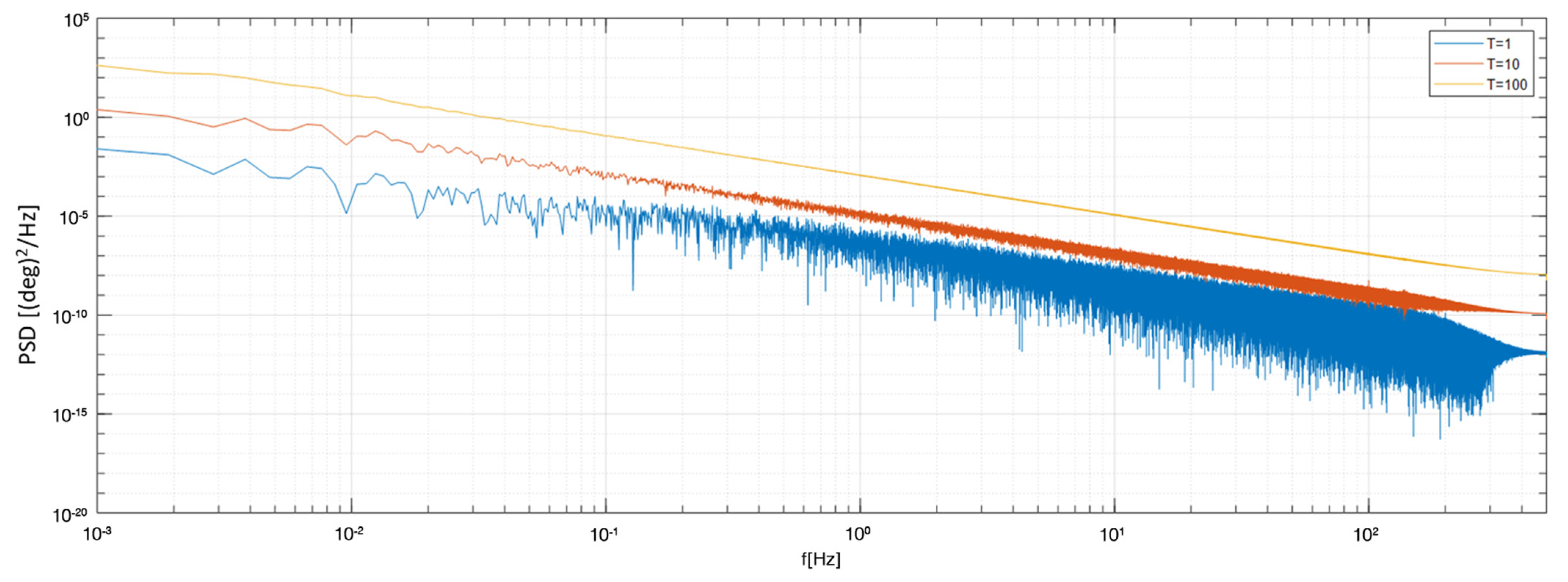
The PSD chart is useful for finding the time constant T of the complementary filter. Figure 12 and Figure 13 present the one-sided PSD of an angle calculated with the use of data from a gyroscope and an ideal measurement of the correction angle. Ideal measurement of correction angle means that only errors of rate gyros are taken into account—properties of gyroscopes are crucial for AHRS behavior. The time constants T of the complementary filter were 1, 10, 100. Temperature was not stabilized, and bias was significant.

As shown in Figure 12 and Figure 13, PSD analysis is useful for the design of an algorithm for the desired system. If the time constant is too high, significant low-frequency (semi-constant) errors of estimated values occur. With a very small time constant, the whole system exhibits high levels of noise. The properties of a whole control system do not depend exclusively on the quality of sensors but are also significantly influenced by the applied algorithm.

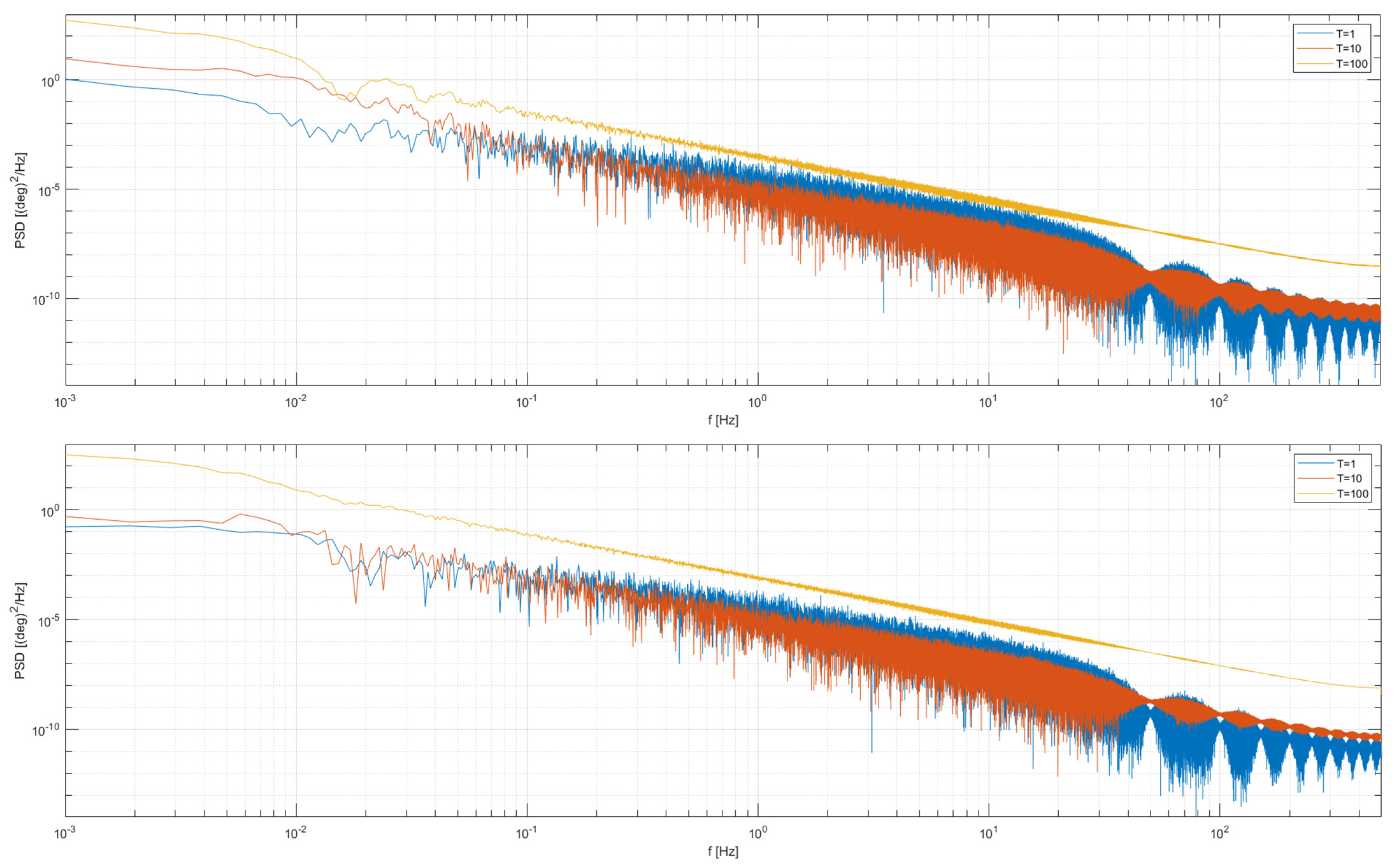
Figure 14 presents the PSD analysis for the calculated roll angle, with different time constants of the complementary filter. In contrast to Figure 12 and Figure 13, the influence of all sensors was taken into account. Similar to Figure 12 and Figure 13, the influence of gyro drift at high time constants may be noted (low frequencies). Also, noises for high frequencies are observable. Frequencies of ca. 100 Hz and higher, for the angle calculated by complementary filters with time constants T = 10 and T = 100, are significantly burdened with, e.g., process noises. In most solutions, these frequencies can be neglected and filtered. As shown in Figure 14, the best time constant within those presented is T = 10. For the complementary filter with time constant T = 1, significant noise is observed in the frequency range of 0.1 to 50 Hz (both for variable and constant operating temperature). Noises in this frequency range are much smaller for the complementary filter with T = 10. For the complementary filter with the time constant T = 100, a significant influence of the gyro drift is observed (frequencies 0.001–0.05 Hz); in comparison with the two other filters, the noise level is higher in the entire frequency range. The discussion above shows that it is possible to use the one-sided PSD method not only for a single sensor analysis but also for the synthesis of the complementary filter for AHRS.

3. Allan’s Method of Variance

Allan variance (AV) is a time-domain signal analysis method originally developed for oscillator stability studies [46,47,48]. Later, it was also adapted to analyze the stochastic drift properties of inertial sensors [23,49,50,51]. In this method, the average relative deviation of the instantaneous value $\overline{y}$ in the time interval $\tau$ is determined (10), and then the standard deviation σ(τ) is calculated in adjacent time intervals (10–13):

$${\overline{y}}_i=\frac{1}{\tau }{{\displaystyle \int }}_{t_i}^{t_{i+1}}x\left(t\right)dt\approx \frac{x_{i+1}-x_i}{\tau }$$

(10)

where $t_i=t_0+i\tau$, $x_i=x\left(t_i\right)—$measurement data, $t_0—$start time.

$$\sigma {\left(\tau \right)}^2=\frac{1}{2}\langle {\left({\overline{y}}_{i+1}-{\overline{y}}_i\right)}^2\rangle$$

(11)

where $\langle \dots \rangle —$mean value of the measurement set i = 1, 2, 3, ..., ∞.

The theory assumes a constant sampling time and an infinitely long measurement data vector. This condition is unachievable in practice and has to be approximated (12). However, taking into account the formula (11), the relation (13) is obtained, where the value N represents the length of the analyzed data sequence:

$$\sigma {\left(\tau \right)}^2\cong \frac{1}{2\left(N-1\right)}{{\displaystyle \sum }}_{i=1}^{N-1}{\left({\overline{y}}_{i+1}-{\overline{y}}_i\right)}^2$$

(12)

$$\sigma {\left(\tau \right)}^2\cong \frac{1}{2\left(N-1\right){\tau }^2}{{\displaystyle \sum }}_{i=1}^{N-2}{\left(x_{i+2}-2x_{i+1}-x_i\right)}^2$$

(13)

In the case of gyroscope studies, the Allan variance can be defined both with respect to the angular velocity $\omega \left(t\right)$ and the angle $\theta \left(t\right)$:

$$\theta \left(t\right)={{\displaystyle \int }}_0^t\omega \left(t\right)dt$$

(14)

The average angular velocity for the period between $t_i$ and $t_{i+1}$ can be expressed by:

$${\overline{\omega }}_i\left(\tau \right)=\frac{{\theta }_{i+m}-{\theta }_k}{\tau }$$

(15)

where $\tau =m{\tau }_0$, ${\tau }_0—$sampling time.

The Allan variance can be defined for the gyroscope data in the form of Relationship (16) or (17):

$$\sigma {\left(\tau \right)}^2=\frac{1}{2}\langle {\left({\overline{\omega }}_{i+m}-{\overline{\omega }}_i\right)}^2\rangle$$

(16)

$$\sigma {\left(\tau \right)}^2=\frac{1}{2{\tau }^2}\langle {\left({\theta }_{i+2m}-2{\theta }_{i+m}+{\theta }_i\right)}^2\rangle$$

(17)

$$\sigma {\left(\tau \right)}^2=\frac{1}{2\left(N-2m\right){\tau }^2}{{\displaystyle \sum }}_{i=1}^{N-2m}{\left({\theta }_{i+2m}-2{\theta }_{i+m}+{\theta }_i\right)}^2$$

(18)

where $N—$length of the measurement set, $m—$number of samples analyzed in the range $\tau$.

When analyzing accelerometer data, the quantities $\omega$ and $\theta$ are replaced by $a$ (acceleration) and $v$ (linear velocity), respectively. In practice, the AV estimation is performed by recording a set of $N$ samples. The set values are then corrected by removing the constant that occurs when the IMU device is turned on. After integrating the angular velocity $\omega$ (or the acceleration a in the case of an accelerometer), AV is determined by (18) [51].

The variance AV of the quantization noise is described by equation (19). It was determined by substituting Function (4) with Formula (20), describing the relation between AV and power spectral density. Equation (20) allows the AV estimate to be derived from the power spectral density. The interpretation of this equation shows that the Allan variance is proportional to the total noise power (in the case of gyroscope angular velocity measurements) filtered by the $\sin 4\left(\pi f\tau \right)/\left(\pi f\tau \right)$² transition function. Note that the filter pass-band depends on the average period $\tau$. This property makes it possible to separate disturbances of various natures by the appropriate selection of $\tau$.

Function (20) allows the determination of the parameters of stochastic disturbances, using the Allan variance plot directly. The value of the quantization noise coefficient is obtained by reading AV over a slope of $-1 \mathrm{dB}/\mathrm{dec}$ at $\tau =\sqrt{3}$ and substituting with Equation (19):

$${\sigma }_{QN}{\left(\tau \right)}^2=\frac{3Q^2}{{\tau }^2}$$

(19)

$$\sigma {\left(\tau \right)}^2=4\underset{0}{\overset{\infty }{{\displaystyle \int }}}{S}_{\omega }\left(f\right)\frac{{\sin }^4\left(\pi f\tau \right)}{{\left(\pi f\tau \right)}^2}df$$

(20)

The value of the coefficient N, related to ARW and VRW noise, is read from the section of the curve with a decrease of −0.5 dB/dec for τ = 1. The Allan variance of ARW and VRW noise is given by

$${\sigma }_{WN}{\left(\tau \right)}^2=\frac{N^2}{\tau }$$

(21)

where N—noise coefficient of the gyroscope.

In the case of sensor drift, the Allan variance is given by the formula

$${\sigma }_B{\left(\tau \right)}^2=\frac{2B^2}{\pi }\left[\ln \left(2\right)-\frac{{\sin }^3\left(x\right)}{2x^2}\left(\sin \left(x\right)+4x\cos \left(x\right)\right)+Ci\left(2x\right)-Ci\left(4x\right)\right]$$

(22)

• where $x=2\pi f{\tau }_0$ and $Ci\left(x\right)=-{{\displaystyle \int }}_x^{\infty }\frac{\cos \left(t\right)}{t}dt$ and
• where B—drift factor (coefficient) and Ci—integral cosine.

The drift coefficient B is interpreted as the smallest value on the Allan variance curve, as the function σ(τ) sums up over a section with a drop of −1 dB, considering both ARW/VRW noise and quantization noise [40]. Relationship (22) is often reduced to the form

$${\sigma }_B{\left(\tau \right)}^2=\frac{2B^2}{\pi }·\ln \left(2\right)$$

(23)

Allan variance for gyroscope or accelerometer noise (RRW/RW) is given by Relation (24). The value of the K factor is read from the AV curve at the point τ = 3 (on the curve with a slope of 0.5 dB/dec):

$${\sigma }_{RW}{\left(\tau \right)}^2=\frac{K^2\tau }{3}$$

(24)

The trend coefficient R is determined from a section with a slope of 1 dB/dec at the point τ = 2. The Allan variance for harmonic signals is given by

$${\sigma }_H{\left(\tau \right)}^2=A^2{\left(\frac{{\sin }^2\left(\pi f_{0\tau }\right)}{\pi f_{0\tau }}\right)}^2$$

(25)

In the examples analyzed in the following sections, devices powered only from DC power sources were used, both during laboratory tests and during practical, in-flight tests. As a consequence, the cumulative AV function for interference is given by

$$\sigma {\left(\tau \right)}^2={\sigma }_{QN}{\left(\tau \right)}^2+{\sigma }_{WN}{\left(\tau \right)}^2+{\sigma }_B{\left(\tau \right)}^2+{\sigma }_{RW}{\left(\tau \right)}^2+{\sigma }_T{\left(\tau \right)}^2$$

(26)

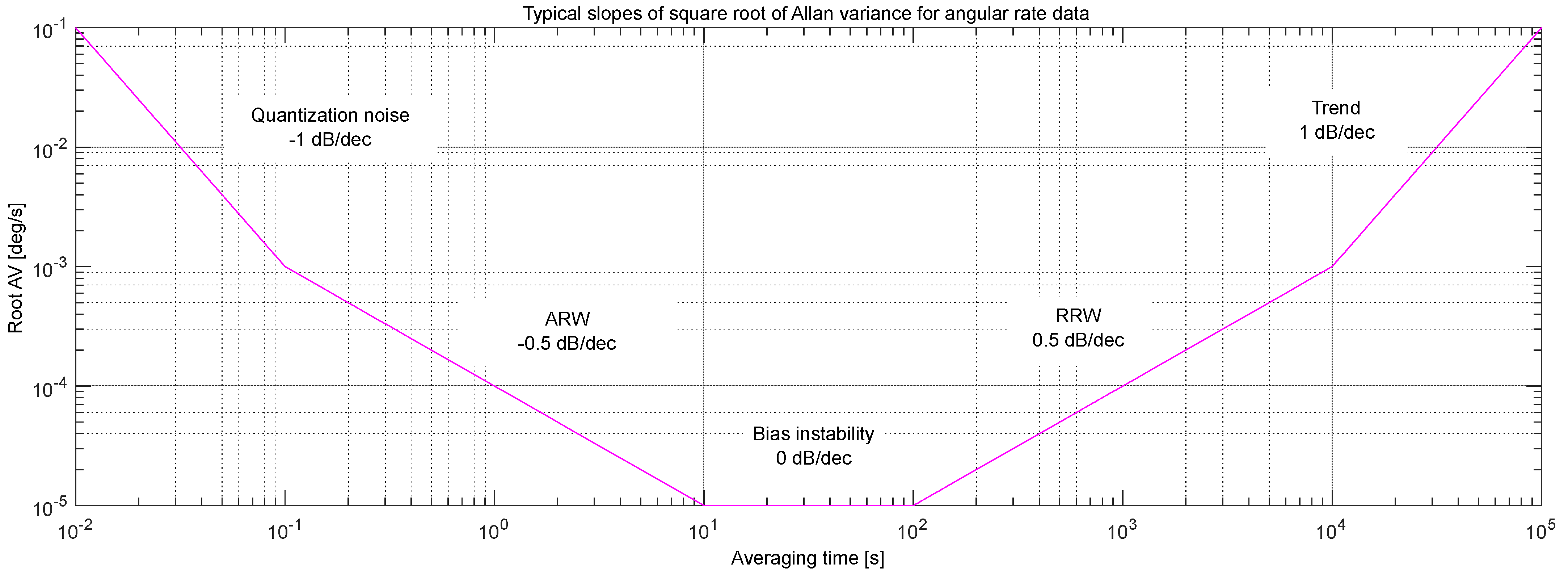
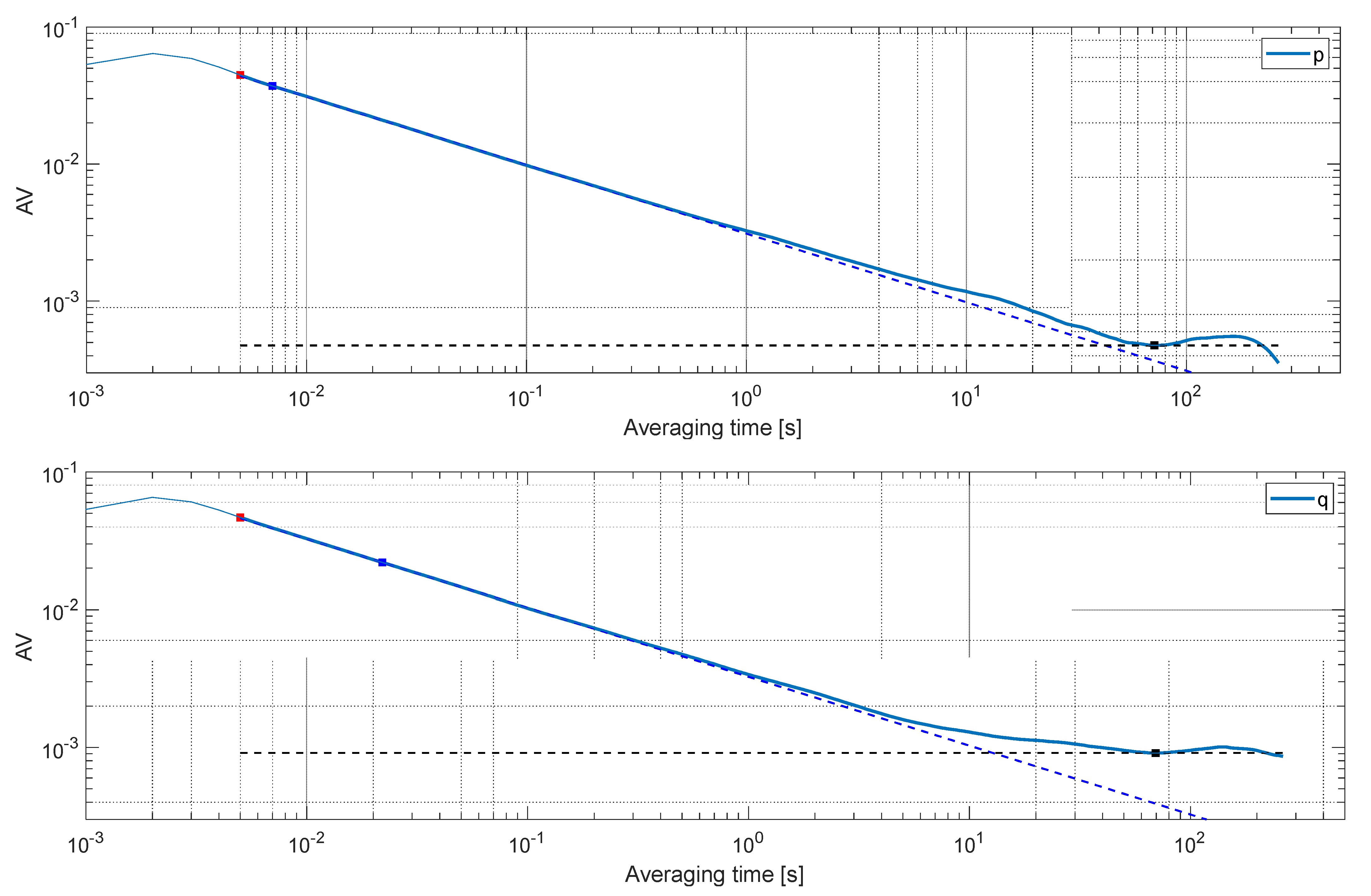
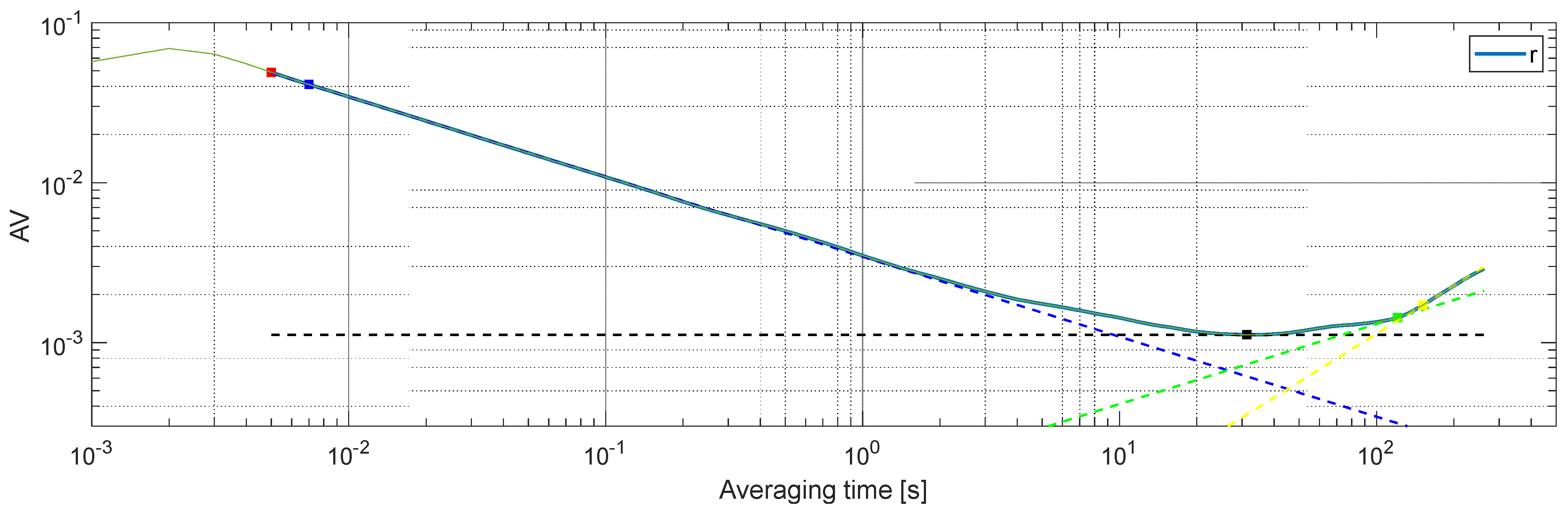
The course of Allan variance for a hypothetical inertial sensor presented in Figure 15 was drawn on the basis of the documentation normalizing the process of testing inertial sensors [23]. Examples of AV graphs obtained for the gyroscopes of the PCIM-01 IMU [42] are shown in Figure 16. AV was determined for the data recorded during the test illustrated in Figure 6. Thus, the AV graphs (Figure 16) can be compared with the PSD graphs presented in Figure 8 (roll angular velocity p) and with Figure 9 (pitch angular velocity q and yaw angular velocity r). When interpreting the graphs, one should pay attention to the fact that the average time in the AV graphs is related to the inversely proportional relationship with the frequency value in the PSD graphs. In the case of the tested sensors, both methods failed to identify the quantization noise characterized by a −1 dB/dec slope in the AV curve (on the left side of the graph) and a +2 dB/dec slope in the PSD graphs (right side of the graph). ARW noise with a decrease of −0.5 dB/dec in the Allan variance plot was identified for all angular velocities. The values of white noise coefficients N determined for gyroscopes using the PSD and AV methods are presented in Table 1 (in the case of this coefficient, the differences reach 25%). For the drift coefficient B, the differences in the results obtained, depending on the method, reach 42%. The noise coefficient of the gyroscope K could not be identified with the AV method in the case of the gyroscope measuring the angular velocity P, while when it comes to the angular velocity R, an approximate value was obtained due to the characteristic slope of less than 0.5 dB/dec in the analyzed range.

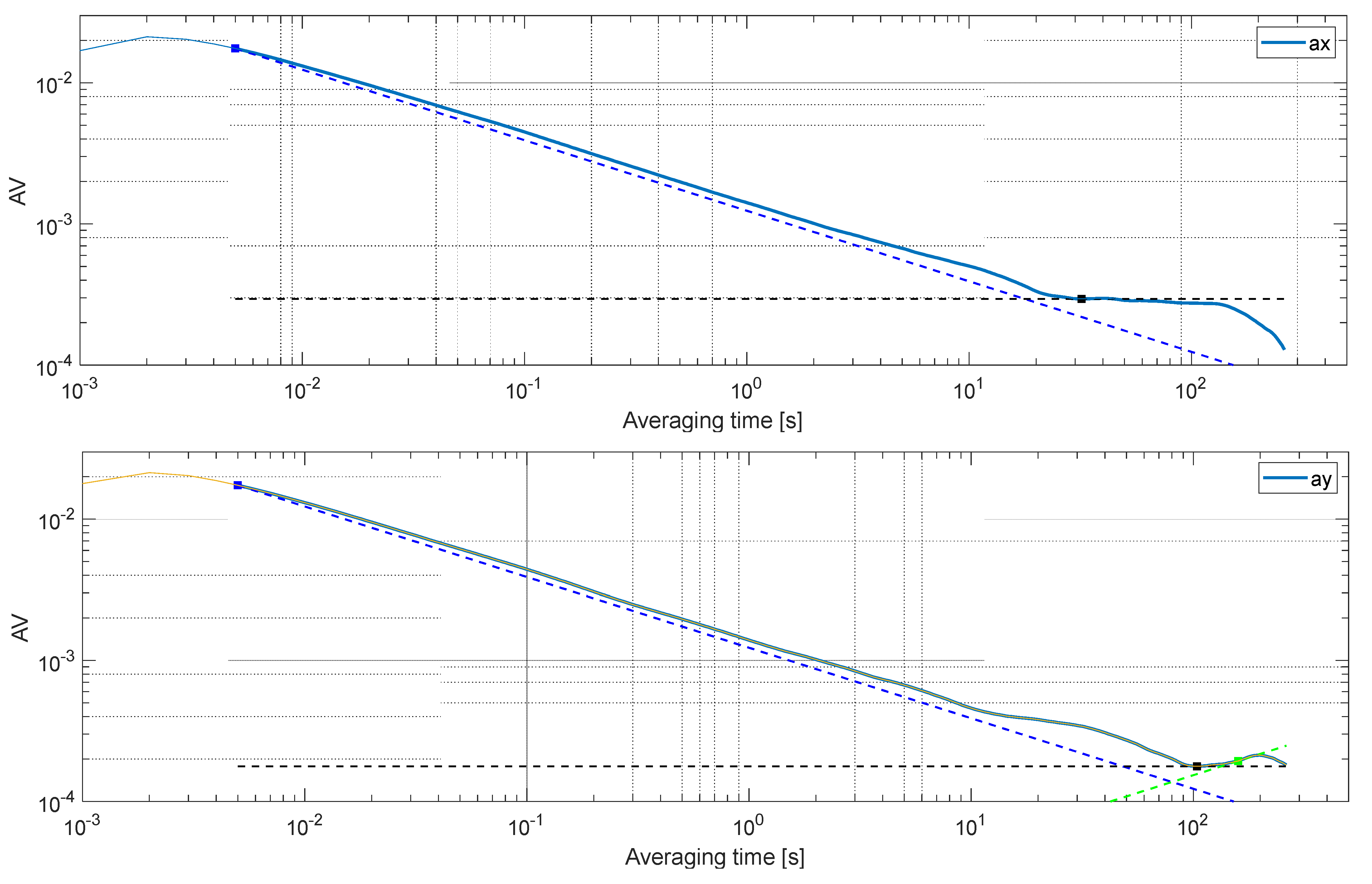
Similar tests were also carried out for the triaxial accelerometer, and the AV results obtained are presented in the graph in Figure 17. The values of the determined noise coefficients are presented in Table 2.

According to the gyroscope manufacturer’s data, the ARW value (white noise coefficient N) determined at a signal sampling frequency of 10 Hz is 0.005 $\mathrm{deg}/\sqrt{\mathrm{s}}$. In the experiment, the signal was sampled with a frequency of 1000 Hz, obtaining ARW values in the range of 0.00305–0.004 $\mathrm{deg}/\sqrt{\mathrm{s}}$ (Table 1).

The root mean square (RMS) noise value read from the catalog data for the tested gyroscope set is 0.06 deg/s for a signal with a bandwidth limited by a digital low-pass filter to 92 Hz. The experimentally determined RMS values for gyroscopes with a stabilized operating temperature, at a sampling frequency of 1000 Hz and a bandwidth limited to 256 Hz, were:

• RMS_p = 0.077 deg/s;
• RMS_q = 0.079 deg/s;
• RMS_r = 0.084 deg/s.

The RMS noise value read from the catalog data for the tested set of accelerometers in the measurement range ±2 g is 0.039 m/s² and concerns a signal with a frequency of 100 Hz. The experimentally determined RMS values for gyroscopes with a stabilized operating temperature, at a sampling frequency of 1000 Hz (bandwidth limited to 256 Hz by a digital filter at the output of the MEMS system), and the measurement range set to ±4 g, were:

• RMS_ax = 0.027 m/s²;
• RMS_ay = 0.028 m/s²;
• RMS_az = 0.040 m/s².

The power spectral density value determined by the manufacturer of the three-axis accelerometer is 0.0039 (m/s²)/Hz^−0.5 for a signal with a frequency of 10 Hz. According to Equation (26), the RMS noise value for this signal is 0.0194 m/s²:

$$RMS=1.57·PSD·\sqrt{f}$$

(27)

The RMS values obtained experimentally are comparable to the manufacturer’s data. However, it should be noted that the sampling frequency of the tested system was 1 kHz, while the catalog data refers only to sampling rates of 10 and 100 Hz. Accelerometers for flight tests were programmed to operate in the range of ±4 g, while the manufacturer, in the available documentation, referred only to the smallest measurement range (±2 g).

Gyroscope sensitivity scale factor variation over temperature according to the manufacturer’s data is ±0.04%/°C (in the range of −40 °C to +85 °C). Accelerometer sensitivity change vs. temperature is ±0.02%/°C (−40 °C to +85 °C, at range 2 g). Change over a specified temperature (component level) is ±0.75 mg/°C for the x- and y-axis and ±1.50 mg/°C for the z-axis.

4. General Method of Wavelet Moments

Allan’s graphical analysis of variance method allows estimation of the parameters of basic stochastic processes by determining linear fragments of the logarithmic AV characteristic with appropriate slopes. In the case of this method, standards and algorithms of conduct have been developed, enabling the separation of individual basic processes [41]. Although this method is widely used, in many cases it turns out to be computationally ineffective [24] and may generate incorrect results [25]. In search of better calculation algorithms and statistical analysis methods, the generalized method of wavelet moments was developed. This technique was developed in 2013 by a team of scientists dealing with the analysis and modeling of complex stochastic processes [24]. It uses a quantity called the wavelet variance (WV), which is the variance of the wavelet coefficients derived from the decomposition of the time series [26]. WV is used for time series analysis in many fields. It enables the decomposition and interpretation of time series variances for different scale values. Papers [24,41] present decomposition algorithms using the Haar wavelet, which acts as a low-pass filter. The wavelet variance is determined using the DWT or MODWT (overlap discrete wavelet transform) algorithms. The estimator of the wavelet variance determined by the MODWT method specifies the relationship

$${{\widehat{\nu }}_j}^2=\frac{1}{T-L_j+1}{\displaystyle \sum }_{t=L_j}^T{W_{j,t}}^2$$

(28)

where T—length of the signal, L_j—length of the Haar filter for the j scale, W_j,t—wavelet coefficients for the j scale, and t—time.

When the wavelet variance estimator for the F_θ, the process is available, then it can be associated with the model expressed by the power spectral density [24]:

$${{\nu }_j}^2\left(\mathit{\theta }\right)={{\displaystyle \int }}_{-1/2}^{1/2}{\left|H_j\left(f\right)\right|}^2{S}_{F_{\theta }}\left(f\right)df$$

(29)

where $\mathit{\theta }$—time series modeling the process, S_Fθ—power spectral density of the process F_θ, and H_j—spectral transfer function of the filter (wavelet) for the j scale.

Relationships (28) and (29) allow the determination of the difference between the estimated WV value and the value resulting from the adopted model. The GMWM method, described in detail in [24], is based on the inverse relationship between wavelet variance and process parameters $\mathit{\theta }\left(\widehat{\mathit{\nu }}\right)$. The estimation of the process parameters in the GMWM method is carried out according to the following formula:

$$\widehat{\mathit{\theta }}=\underset{\theta ϵ\mathsf{\Theta }}{\mathrm{argmin}}{\left(\widehat{\mathit{\nu }}-\mathit{\nu }\left(\mathit{\theta }\right)\right)}^T\mathbf{\Omega }(\widehat{\mathit{\nu }}-\mathit{\nu }\left(\mathit{\theta }\right))$$

(30)

where $\widehat{\mathit{\nu }}={\left[{\nu }_j^2\right]}_{j=1,\dots ,J}$—the vector of estimated WV, $\mathit{\nu }\left(\mathit{\theta }\right)={\left[{\nu }_j^2\left(\mathit{\theta }\right)\right]}_{j=1,\dots ,J}$—WV resulting from the model, and Ω—positively defined weighting matrix.

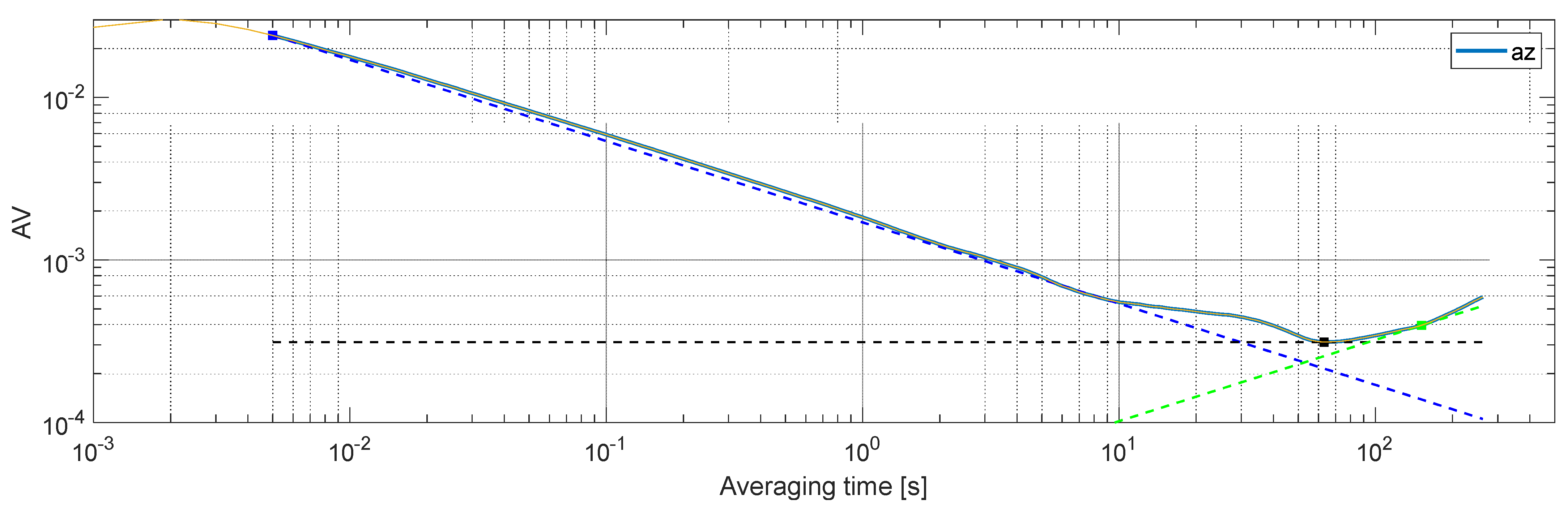
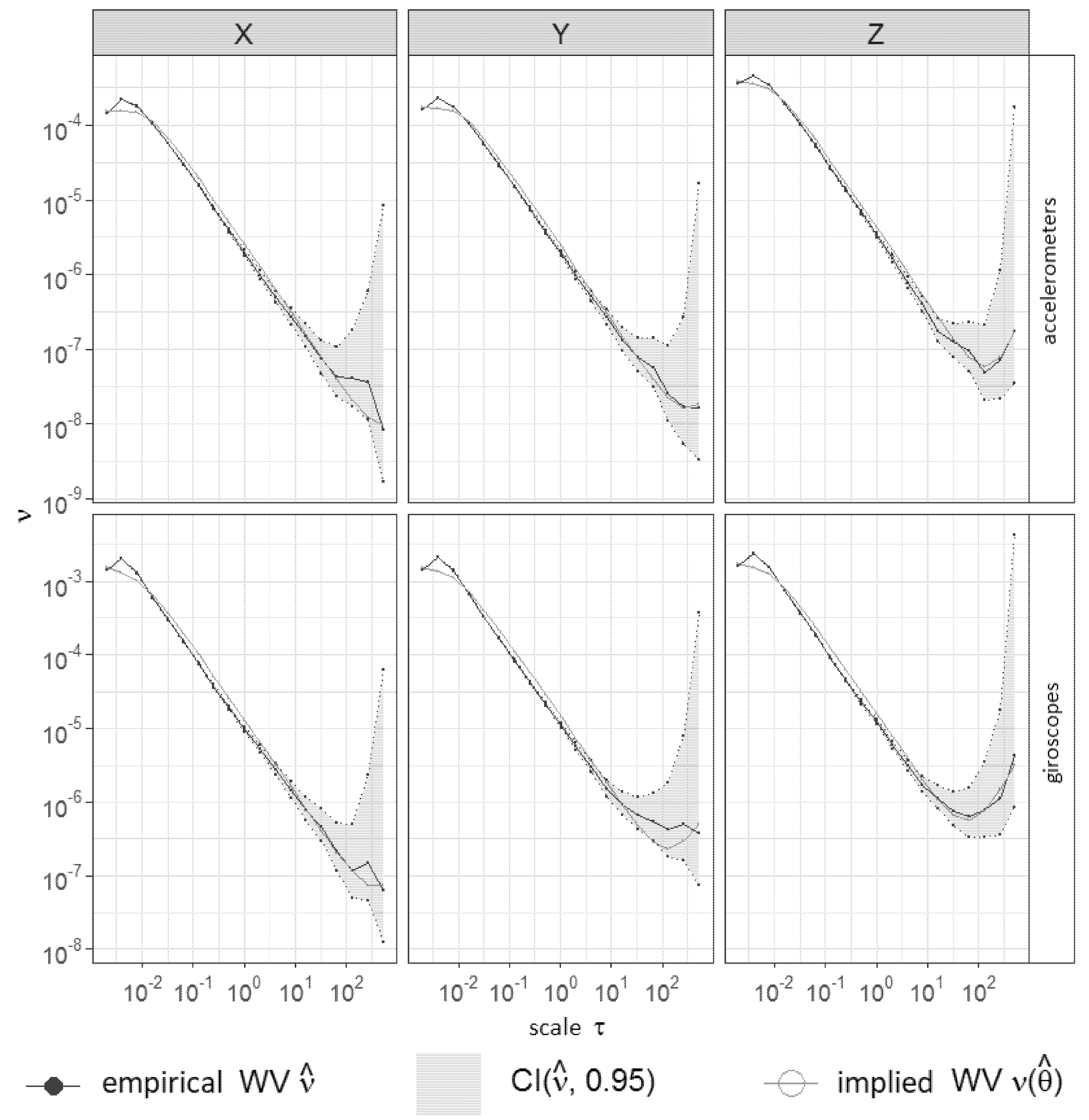
Equation (30) enables minimization of the difference between the estimated and modeled wavelet variance of the process due to the appropriate selection of the value of the weighting matrix Ω (e.g., by the least squares method). The main goal of the GMWM method, however, is to properly match the WV of the process and its model. Figure 18 shows the results of the auto.imu function (R2 environment, GMWM library [24]), which enabled the determination of WV and the automatic selection of parameters for the models of inertial sensors of the PCIM-01 IMU. The function was called with the parameter model = AR1() + WN() + RW() + DR(), indicating the modeled stochastic processes: first order autoregressive process (AR1), white noise (WN), sensor drift (DR), and noise gyroscopes/accelerometers (RW). The wavelet variance based on the Haar function becomes equivalent to the Allan variance ($\sigma =2\nu$) when its value is doubled.

Determining the value of the white noise coefficient (N) using the GMWM is carried out with the method of direct matching of the wavelet variance of the model and the real signal, taking into account the equation

$$N=\sqrt{WN·T_s}$$

(31)

where N—the white noise coefficient of the analyzed process, WN—the noise coefficient for the discrete model resulting from the GMWM, and T_s—sampling time period.

The drift coefficient (B) was determined based on the value of the local minimum from the wavelet variance for 100 s averaging times

$$B=\sqrt{2·W{V}_{min}}$$

(32)

where WV_min—minimum value of wavelet variance in the averaging interval determined by the expert method.

The values of the K coefficient were determined using the graphical method by fitting the obtained logarithmic characteristic WV and a line with a slope of 1 dB/dec. In order to compare all three discussed methods (PSD, AV, and GMWM), the values of coefficients N, B, and K determined for the set of inertial sensors of the PCIM-01 IMU of the PRP-W2 system are summarized in Table 1 and Table 2. The results obtained for GMWM are comparable to AV, but the values resulting from the use of GMWM are not affected by errors related to, for example, the graphic fitting of curves. Moreover, they result directly from the values obtained for the models (this applies in particular to the N and B coefficients).

5. Conclusions

Due to PCIM-01–inertial measurement unit module [42] construction, the tested MEMS accelerometers enable practical measurement of vibrations with frequencies ranging from tenths of a hertz to even 1 kHz. MEMS gyroscopes can be used to measure angular velocities and, indirectly, angular oscillations in similar frequency ranges [42,52]. MEMS inertial sensors, although unfortunately burdened with serious stochastic errors, are widely used not only in commonly used devices but also in such safety-critical solutions as AHRS. The aim of this article was to present the stochastic properties of sensors used in the flight parameter recording system of a light aircraft. The article discusses the issue of the influence of the stability of the sensors’ operating temperature on the obtained time characteristics and on the power spectral density of the output signals. The frequency characteristics pointed to the areas related to the temperature drift and to the electro-mechanical noise of the sensors. The stochastic properties of MEMS accelerometers and gyroscopes under stable operating temperature conditions were additionally assessed using power spectral density, Allan variance plots, and the generalized method of wavelet moments. The stochastic properties of MEMS sensors determined by the PSD, AV, and GMWM are convergent. However, only the results achieved with the GMWM method enable direct verification of the models obtained.

The white noise N parameters determined with different methods have similar values, and the maximum difference for the accelerometer in the z-axis, during the warming-up process (Table 2), was 21% of the relative standard deviation (RSD). In the majority of remaining cases, the variance was not higher than 10%. Allan’s method of variance is the easiest way to determine the drift coefficient, as the drift is determined on the basis of the lowest point on the characteristic curve. In turn, the PSD method, for which it is necessary to adjust a line with a −1 dB/dec deviation to irregular characteristics, seems to be the most problematic. The results obtained with the AV and GMWM methods are often identical. However, when all three methods for drift determination are compared, the greatest difference, i.e., 109% of RSD, was observed for the accelerometer in the z-axis under stable operating temperature conditions (Table 2). In some cases, it was impossible to determine the Brown noise because it occurred in negligible values. When the noise was higher, the AV and GMWM methods were highly effective, and the results obtained were very similar or identical (e.g., with accelerometers at stabilized operating temperature, Table 2)

The analysis of the stochastic parameters of gyroscopes and accelerometers is helpful in the selection of adequate sensors and in the process of AHRS algorithm synthesis. The results obtained with the PSD, AV, and GMWM methods are complementary, as well as being mutually verifiable, especially in the case of AV and GMWM methods. With precise information on the stochastic parameters of sensors, it is possible to determine types of phenomena that can be analyzed with the help of the results obtained. In the case of flight parameter recorders, it is also possible to determine incidents that can be detected with a certain sensor unit.