Climatology of 557.7 nm Emission Layer Parameters over South-East Siberia, Observations and Model Data

Abstract

The paper deals with long-term means of 557.7 nm atomic oxygen airglow intensity (OI) and air temperature within the mesopause over the southern regions of East Siberia. Data on temperature and emission parameters were obtained with a SABER radiometer, KEO Scientific “Arinae” Fabry–Pérot interferometer, SATI spectrometer and NRLMSIS model over the Tory Geophysical Observatory (52° N, 103° E). Annual variations of 557.7 nm emission intensity and temperature obtained in observations differ from model approximations. Potential reasons for the discrepancies revealed are discussed.

1. Introduction

Atomic oxygen is integral to the photochemistry and energy balance in the mesosphere–lower thermosphere (MLT) region. The maximum concentration of atomic oxygen is observed at altitudes of ~100 km. Emission in line 557.7 nm occurs in the recombination of atomic oxygen (is caused by the recombination of atomic oxygen), which is formed due to the photo dissociation of molecular oxygen by solar UV (ultraviolet) emission [1]. Monitoring 557.7 nm atomic oxygen emission is one of the basic ways to investigate MLT thermodynamic conditions. In the entire nighttime airglow spectrum, 557.7 nm emission was the first one revealed at the beginning of the last century [2]. Nowadays, it is the most well-understood nightglow line. However, there are a number of unsolved problems; for example, features of diurnal and seasonal variations in 557.7 nm emission intensity (I 557.7 nm) at different latitudes are not entirely explained. Low latitudes, for which long-term observations from geostationary satellites have been accumulated, are the most well-studied [3,4]. At middle and high latitudes, I 557.7 nm is mainly monitored at different ground-based stations or using limb-scanning satellites [2,5]. Long-term studies of I 557.7 nm show the existence of pronounced seasonal dependence and inter-annual variations [6,7]. The annual component of I 557.7 nm variations is the most significant mode, and its amplitude increases with latitude. The amplitude of the semiannual component of these emission variations is far weaker than the amplitude of the annual component, and it is the strongest over the equator and decreases with latitude [8]. Paper [2] shows that the amplitude of the green line annual component at 7–44° N is within 10–30%, with smaller amplitudes at low latitudes. The amplitude of semiannual variations also varies with latitude; it decreases with latitude from 37% at low latitudes to ~10% at mid-latitudes. Using 557.7 nm photometry data over Kiso for 1979–1994, the authors of [9] showed the existence of two seasonal peaks: one in June and the other one in October.

In the tropical region, semiannual variations in 557.7 nm emission were seen from WINDII satellite measurements, in measurements with ground-based photometers and in the TIME-GCM model [10]. However, for mid-latitude regions, the semiannual component was noted in [10] based on satellite data only at 96 km at 20:00 LT; it weakened overnight and almost disappeared by 02:00 LT. Based on long-term data on I 557.7 nm over the Tory Geophysical Observatory (GPO), paper [11] demonstrates the existence of three I 557.7 nm maxima during equinox periods in February–March and October, and in June, the October maximum has the greatest amplitude. The minimum of I 557.7 nm was observed in April. The following can be referred to as the potential mechanisms determining the features of seasonal variations in I 557.7 nm: variations in global atmospheric circulation at MLT heights that provide the atomic oxygen transfer in the upper atmosphere, oxygen layer vertical motions and temperature variations at the emission level.

Due to transition in the excited oxygen atom $O({}_{}{}^{1}S-{}_{}{}^{1}D)$, 557.7 nm emission occurs. The 4.2 eV excited oxygen atom $O\left({}_{}{}^{1}S\right)$ results from triple collisions with the participation of atomic oxygen (the Barth mechanism) and includes the following stages:

$$O+O+M\to O_2^{\ast }+M$$

(1)

$$O+O_2^{\ast }\to O{(}^{1}S)+O_2$$

(2)

Knowing the atomic oxygen concentration per volumetric unit, and the flow rate (1), (2), we can estimate the number of 557.7 nm photons emanating from a volumetric unit per unit time.

Moreover, the hydroxyl airglow is related to the atomic oxygen chemistry via ozone by the following reaction:

$${H+O}_3\to {OH}^{\ast }+O_2$$

(3)

In this case, ozone is generated from oxygen atoms by means of a triple collision reaction:

$${O+O}_2+M\to O_3+M$$

(4)

To determine the atomic oxygen concentration in the night using the hydroxyl airglow, Mlynczak et al. (2013) [12] assumed that the ozone production due to recombination (4) is balanced by its loss resulting from reaction with atomic hydrogen (3). Therefore, the hydroxyl emission intensity observed, e.g., with a SABER instrument, is directly proportional to its formation rate, hence, directly proportional to atomic oxygen concentration. Thus, data obtained through hydroxyl observations can be used to estimate the concentration of atomic oxygen and the synthesis of 557.7 nm airglow intensity and to further study the regional climatology of this airglow line.

In a sense, this paper continues the cycle of studies [11,13,14] carried out in previous decades in the Tory GPO, only with the use of different ground, satellite and model data. The study is purposed to investigate the features of seasonal variations in MLT temperature and 557.7 nm emission characteristics over the Tory GPO and to compare the results from data obtained with a SABER radiometer, KEO Scientific “Arinae” Fabry–Pérot interferometer, SATI spectrometer and the NRLMSIS model.

2. Data Sources

In our study, we used data from the SABER radiometer aboard the TIMED satellite (http://saber.gats-inc.com/ accessed on 18 April 2023). SABER conducts global measurements of atmospheric parameters with a 10-channel broadband infrared radiometer using the method of Earth’s limb scanning within the spectral range from 1.27 to 17 μm [15]. These measurements are employed to plot vertical profiles of kinetic temperature, pressure, geopotential height, $O_3$(ozone) mixing ratio, OH (hydroxyl) emission intensity and $O_2$(molecular oxygen) concentration. To compute the height profile of the upper atmosphere I 557.7 nm, we used the height profile of atomic oxygen concentration and filtered data over the area of a 700 km radius with the center at GPO Tory (51°48′ N 103°04′ E). More details of SABER data collection and the spatial filtration and calculation of 557.7 nm intensity are given in [16].

The KEO Scientific “Arinae” Fabry–Pérot interferometer (FPI) is in the ISTP SB RAS GPO (Institute of Solar-Terrestrial Physics Siberian Branch of Russian Academy of Sciences Geophysical Observatory) near the Tory settlement in the Republic of Buryatia, Russia. The interferometer detects temperature and wind velocity from Doppler broadening and a shift of natural nightglow spectral lines. We use data obtained using the 557.7 nm line emitted by atomic oxygen in a ~10 km thick layer at the altitude of 90–100 km above the Earth’s surface. Unlike satellite instruments, the ground-based interferometer detects the airglow of the entire layer, without separation according to altitudes. Therefore, the obtained parameters (airglow intensity, temperature, wind) represent some integral values averaged over the entire airglow layer. The technique of detecting atmospheric parameters using the FPI is presented in [17].

The SATI spectrometer is made on the basis of the ISP-51 serial spectrometer and VIDEOSKAN-285 camera. ISP-51 is a three-prism spectrometer with glass optics, which comprises two identical 60° prisms and one constant-deviation prism. The prisms are made of AR-coated flint glass and allow the use of the 360–1000 nm spectral band. Just like an interferometer, a spectrometer observes integral airglow intensity. In this paper, we use data on I 557.7 nm as received from this device.

In our study, we use model NRLMSIS 2.0 developed by a team of authors in [18] on the basis of model NRLMSISE-00. NRLMSIS 2.0 employs rocket and satellite measurements and data from incoherent scatter radars. The model calculates concentrations of He, O, $N_2$, $O_2$, Ar, H, N, total mass density and neutral temperature at heights up to 1000 km from the Earth’s surface.

The calculation of nightly averaged values within the area where the SABER data were taken was performed for tangent-point solar-zenith angles over 94 degrees. For NRLMSIS and FPI data, it was performed for nightly data between civilian twilight (solar angles over 99 from zenith).

3. Methods

For proper comparison of temperatures obtained from different data sources, they should be reduced to one parameter and synchronized. Integral airglow intensity observed with a ground-based instrument cannot be transformed to height profile; therefore, to compare airglow intensity from SABER data and simulation results with that from ground-based instruments, it should be reduced to arbitrary units—Rayleighs. Temperature profiles obtained with simulation and the satellite instrument should also be averaged with the weights equal to airglow intensity in order to obtain integral characteristic—effective temperature [16,19]—which shall be further compared with the interferometer observation results. Finally, due to the fact that observations with ground-based instruments are only possible in the night, daylight hours should be excluded from time series of satellite and model data. The resultant data series shall be brought to a common form. Gaps in data series due to inappropriate observational conditions or technical problems, data dispersion due to weather conditions and equipment noise impede comparison, e.g., of the studied parameters’ annual dynamics. Hence, we compared time series of nighttime means and monthly means of the studied parameters. The time series were preliminarily averaged over 2017–2021.

3.1. SABER

Intrinsically, atomic oxygen causes the occurrence of 557.7 nm airglow; hence, atomic oxygen concentration that can be obtained from SABER data is the basis to estimate airglow intensity from satellite data. The technique described in [12,20] allows obtaining height profiles of atomic oxygen concentration from height profiles of hydroxyl, temperature, ozone and atmospheric density. After that, one can obtain a height profile of the 557.7 nm volume emission rate (VER) based on data presented in [21], which describes the method of atomic oxygen concentration calculation from the known 557.7 nm intensity. For further comparison with data from ground-based instruments, the resultant height profile of volume emission rate must be converted to Rayleighs (${10}^{-6}photons/\mathrm{c}{\mathrm{m}}^2/\sec )$. To do this, the below expression can be used:

$$R={10}^{-6}\times \sum _i^N{I}_i\mathsf{\Delta }h\times {10}^5=I_S\mathsf{\Delta }h\times {10}^{-1}$$

(5)

where $I_i$ is the volume emission rate ($photons/\mathrm{c}{\mathrm{m}}^3/\sec )$ for each level ($i$), N is the number of levels in height profile, and h is the layer thickness in kilometers. Such transformations can be found in [22], for example. In our study, the layer thickness $h$ is 85–100 km.

In addition, using height profiles of temperature and I 557.7 nm at 85–100 km, we calculated effective temperature from SABER data. The effective temperature was calculated with the intensity profile shifted two kilometers up relative to the temperature profile, because according to previous results, seasonal variations in effective temperature show the best match with seasonal variations in temperature recorded using FPI [16]. The same paper [16] describes in detail the technique of synthesizing intensity and deriving effective temperature.

If only integral parameters are compared, it reduces the research potential of the SABER dataset, because in this case, information on vertical dynamics of the parameters in question will not be used. Therefore, in addition to integral values, it is useful to extract information about extreme values from height profiles. In this study, we shall also use data on heights of temperature minimum, maximum atomic oxygen concentration and 557.7 nm airglow intensity maximum.

3.2. Fabry–Pérot Interferometer

Figure 1 shows the comparison of variations in I 557.7 nm synthesized from SABER data and variations in integral intensity observed with FPI. Figure 1 presents day-to-day variation of I 557.7 nm average from 2017 to 2021. It should be noted that at some time points, there are similar variations of I 557.7 nm from different sources, up to interdiurnal variations, for example, from day 40 to 130 or from day 330 to 365. The results of I 557.7 nm measurements obtained with Fabry–Pérot interferometer are given in arbitrary units, because the equipment evaluating the light flux intensity was not calibrated. Arbitrary units of intensity observed with the interferometer can be converted to Rayleighs using SABER data for the periods when intensity variations show the best similarity.

Figure 2 shows the scatter diagram for I 557.7 nm series by FPI and SABER for days 0–125 and 325–365 of year (best similarity time). Despite the existing dispersion, positive correlation of the two studied series is well-defined, and the Pearson correlation coefficient of the series equals 0.471. The method of determining the intensity from interferograms assumes background subtraction [17]; therefore, for the suggested interferometer calibration, correlation of FPI and SABER intensities can be considered to be linear but without the zero shift. The linear regression line of two datasets that runs through the origin is also given in the scatter diagram. Tangent of the line inclination angle 6.322 R/arb. unit (Rayleighs/arbitrary units) will further be used to convert the interferometer arbitrary units to Rayleighs.

3.3. NRLMSIS

Within this study, we simulated I 557.7 nm airglow using data of NRLMSIS 2.0 model. Intensity is calculated using a similar technique [16], but in this case, concentrations of atomic and molecular oxygen were taken from NRLMSIS 2.0 data over the 2017–2021 period for 80–120 km altitudes with 1 km increment and time resolution of 0.25 h. From the data derived, we extracted time intervals corresponding to the FPI nighttime observations. Then, intensities were averaged over 2017–2021 for each night of year and month. We used the intensity synthesized this way to calculate it in Rayleighs using expression (1) and to define the intensity-weighted effective temperature of a layer in height profile section. In addition to calculation of the above parameters, the NRLMSIS 2.0 model was employed to obtain the dynamics of altitudes of minimum temperatures, averaged concentration of atomic oxygen and altitudes of I 557.7 nm airglow maxima.

4. Results

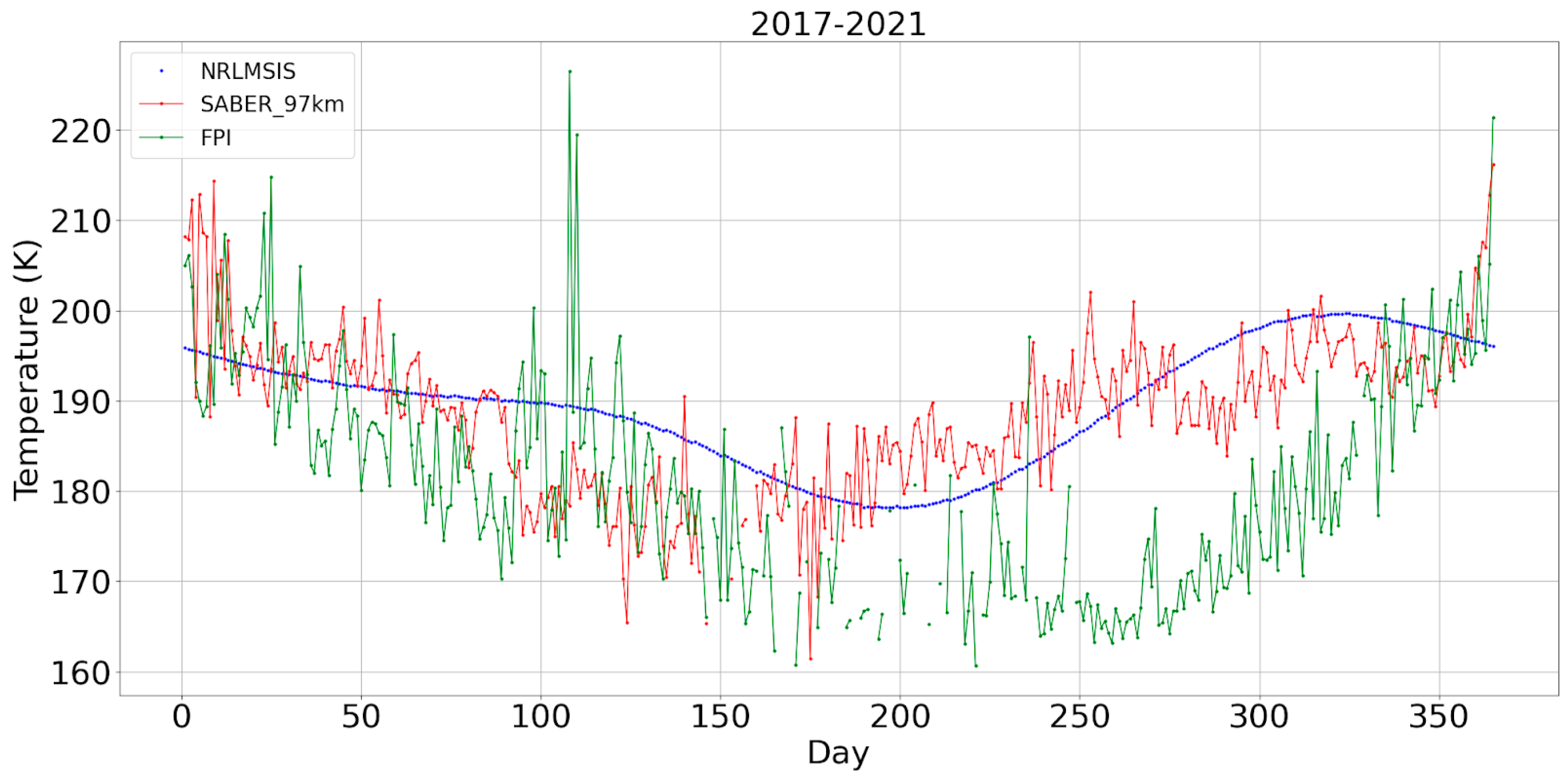
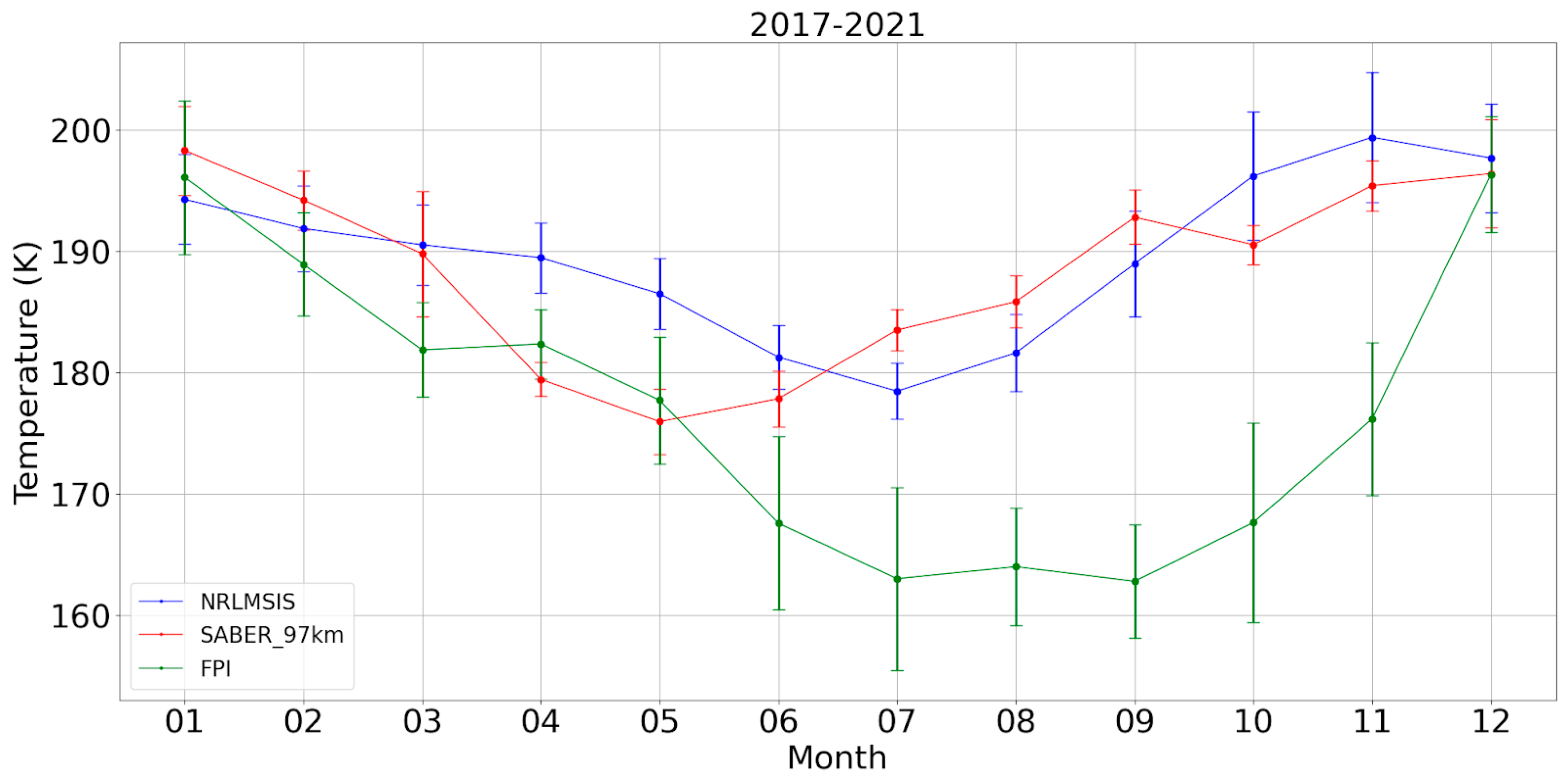
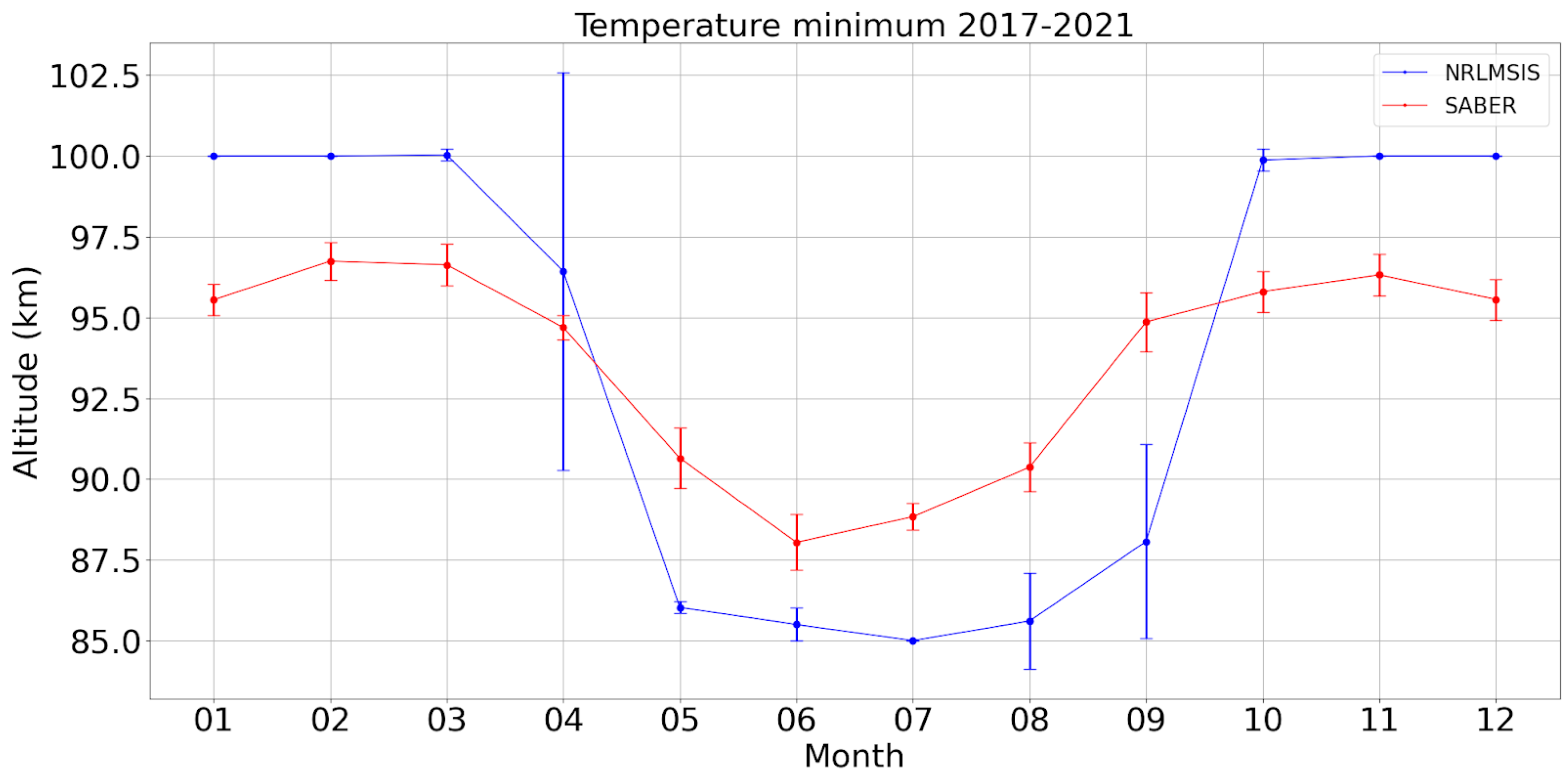
4.1. Temperature

The mesopause is colder in summer than in winter. It is related to atmospheric circulation at the mesopause altitudes causing the upwelling at the summer pole and downwelling at the winter pole. The ascending air expands adiabatically and cools down, which leads to the cold summer mesopause and vice versa—the air descent leads to air compression and temperature rise in the winter mesopause related to it [23]. In the mesosphere, annual circulation is associated with the dissipation of gravity waves driving the meridional circulation [24].

Figure 3 presents annual variations in average nighttime effective temperature in the mesopause region as obtained from the SABER, FPI and NRLMSIS model for 2017–2021 at the altitudes of 85–100 km over the south of East Siberia. Figure 4 shows annual variations in the monthly average nighttime effective temperatures in the mesopause region, the same as Figure 3.

Figure 3 and Figure 4 show that the lowest temperatures are seen in summer (~160–180 K), and the highest are seen in winter (~200 K) from empirical and model data. However, according to model data, the seasonal temperature decrease is smoother, while satellite and ground data show higher rates of temperature decrease. The temperature decrease from interferometer data near the hundredth day of the year is followed by strong variations, during which some nighttime means can exceed winter temperatures (Figure 3). These variations in the daily averaged values of I 557.7 according to the FPI lead to the fact that instead of a seasonal decrease in I 557.7 from winter to summer, it slightly increases in April. Minimal monthly average effective temperatures in the mesopause region are reached in May from SABER data (175 K) and in July from NRLMSIS data (178 K), after which the temperature begins to rise. According to FPI data, the lowest temperatures are reached in July and remain almost the same (165 K) until September (Figure 4). Due to data dispersion, these points in time are difficult to detect from Figure 3, but the difference between temperatures in the summer–autumn period is well-defined. The rates of temperature rise from model and satellite data in the summer–autumn period are approximately the same, while according to interferometer data, temperature begins to rise significantly only in autumn. The difference in temperature from different sources amounts to ~20 K and occurs in September–October. According to interferometer data, in autumn, temperature growth begins in October, the growth rate being significantly higher than in model and satellite data. As a result, the effective temperatures reach the same values for all three instruments in wintertime.

Figure 5 presents the comparison of temperature minimum altitudes from data by SABER and the NRLMSIS model (there are no interferometer data on the graph since it measures integral parameters of the atmosphere). The annual dynamics of the temperature minimum position from height profiles from the satellite instrument and model are consistent. It should be noted that according to SABER, the amplitude of variations in nighttime mesopause altitude is a little less than 10 km, and according to the model, this value change is 15 km.

Thus, the temperature dynamics and the temperature profile (temperature minimum) in general correspond to the modern concept of the mesopause temperature regime. The revealed differences are discussed below.

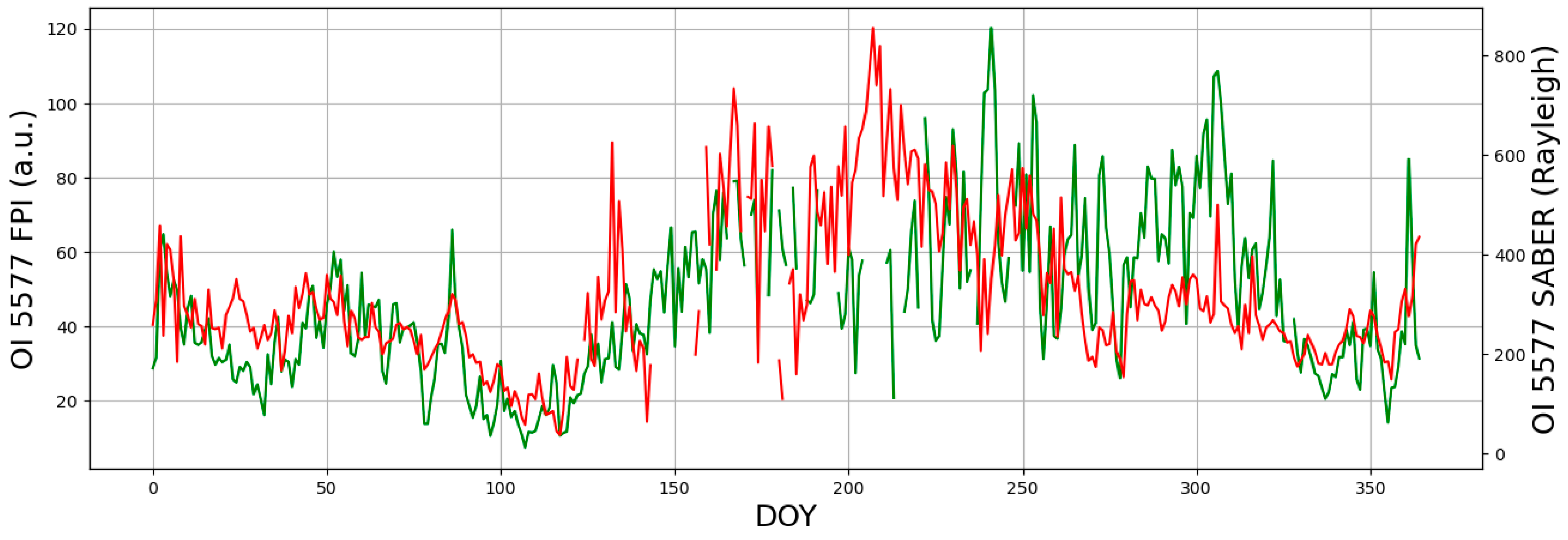
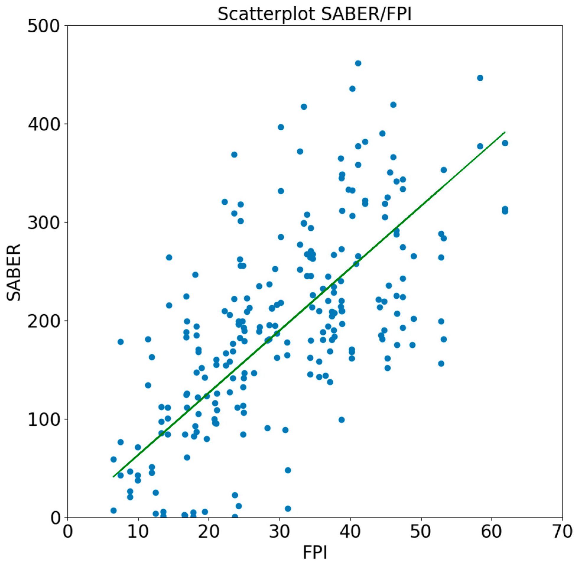
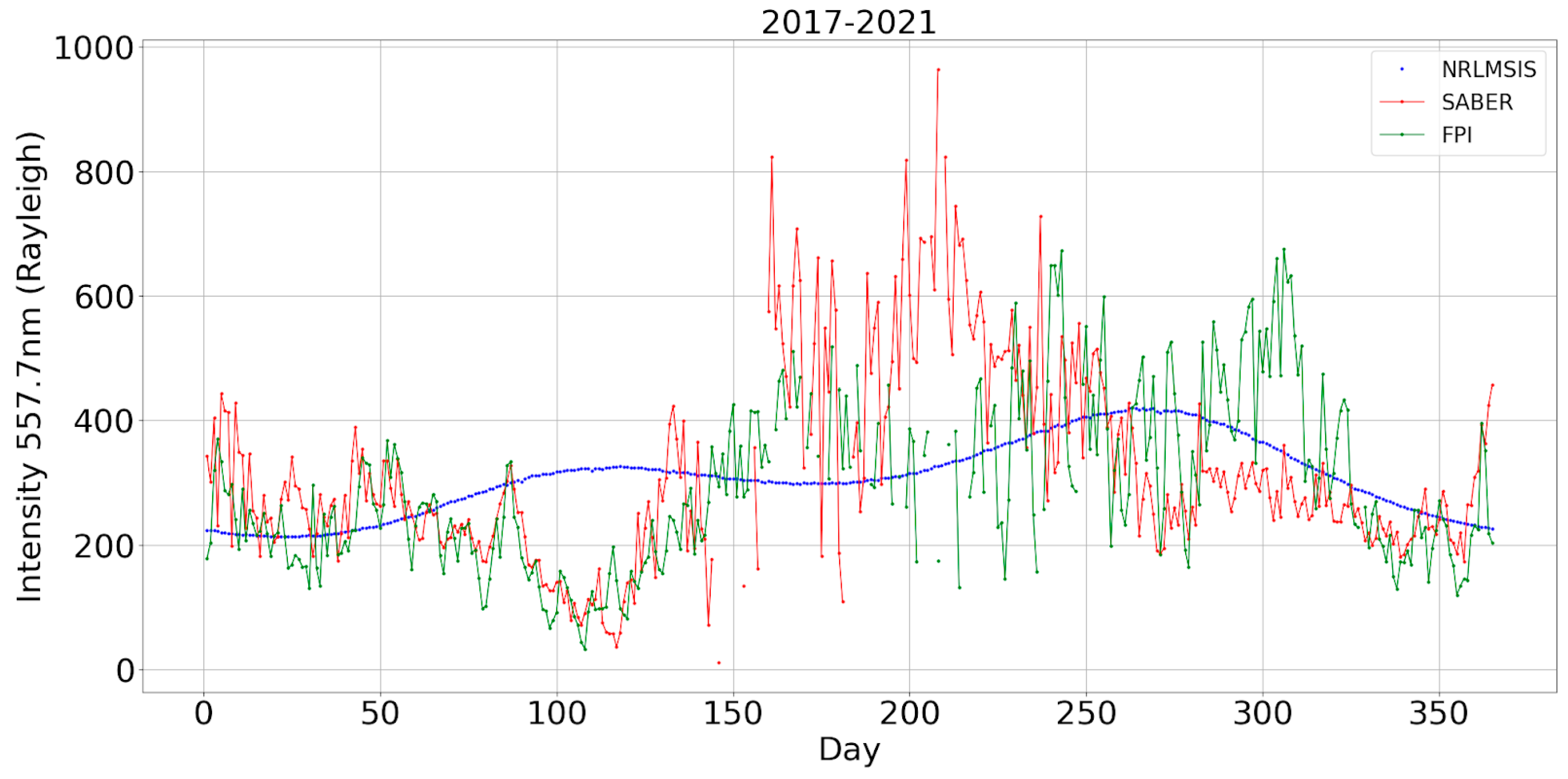
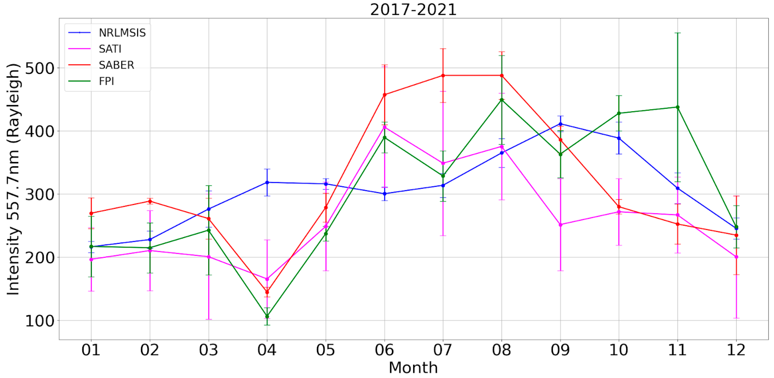
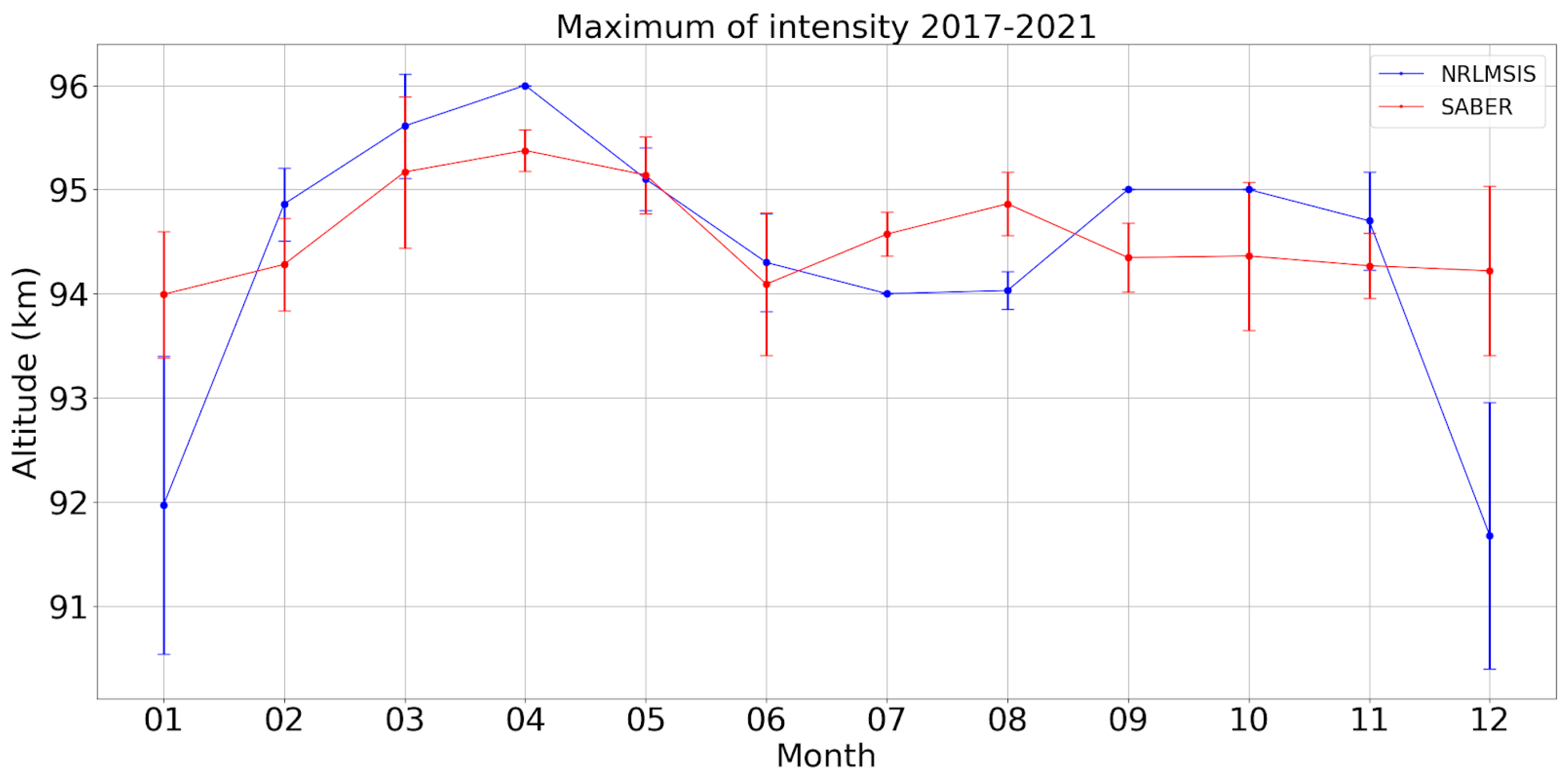
4.2. Intensity 557.7 nm

Figure 6 demonstrates annual variations in average nighttime I 557.7 nm airglow as obtained from the SABER, FPI and NRLMSIS model for 2017–2021 over the south of East Siberia. Figure 7 shows annual variations of monthly average nighttime intensities, the same as Figure 6. Minimal values of I 557.7 nm are observed in the winter–spring season, and maximal I 557.7 nm are essentially seen in summer and autumn. Seasonal variations of intensity are actually the same for different instruments from early winter to early summer and different in summer and autumn (Figure 6). Winter airglow intensities are ~200–300 R, the intensity begins to decrease as the spring season begins, and minimal values of ~100 R are reached in April. From spring to summer, we can see a sharp growth of intensity, up to 400 R in early summer, after which a convergence in data from different instruments begins. From satellite data, the intensity continues to enhance to maximal values of ~500 R in July–August, and from ground data, the intensity begins to vary within 300–450 R. According to all instruments, intensity starts to decrease in August–September, but from interferometer data, it increases again in October and November, while SATI and SABER show a decrease in the intensity. The greatest discrepancy in the observed intensity is seen in November amounting to almost 200 R. As winter sets in, I 557.7 nm from all instruments become almost the same, reaching 200–300 R. According to NRLMSIS data, intensity variations do not exceed 200 R throughout the year. It should be noted that except for the April minimum, at all other times, the model intensity is consistent with the average monthly values obtained with the interferometer. Considerable differences are seen in June and November. In addition, the intensity obtained using the model has a local maximum in spring, when we observe the global minimum of intensity according to all instruments in question.

Figure 8 shows the comparison of intensity peak positions in the height profile averaged over the month from data by SABER and NRLMSIS. One can note that from January to June, the behavior of both plots is relatively similar, the height of the airglow maximum growing from January to a maximum of 95.5–96 km in April and going down to summer minima of ~94 km in April–June. From satellite data, in the second half-year, the maximum altitude of the airglow peak of ~95 km is reached in August; according to model data, it is reached in September–October. December and January monthly average altitudes of the intensity maximum are significantly lower from model data than those from satellite data (92 and 94 km, respectively).

Another interesting result is the asymmetric behavior of intensity and temperature related to changes in the circulation pattern. During circulation restructuring in spring, we can see a significant decay of airglow intensity and considerable temperature variations. In autumn, the circulation pattern changes without critical intensity decreases and temperature variations. The shift in the altitude of the intensity maximum to August in Figure 8 should indirectly spur the researchers to further search for the reason for this asymmetry.

5. Discussion and Conclusions

5.1. Temperature

The observed temperature behavior in the winter and spring seasons distinguishes the mesopause annual temperature variations above Eastern Siberia from the normal one. It can be assumed that this behavior is driven by the influence of processes developing in the underlying atmospheric layers. Winter is characterized by a high frequency of sudden stratospheric warmings, which occur and rapidly develop over Siberia. These processes might cause significant variations in average nighttime temperatures and a related slowdown of the decrease in monthly average temperature [25].

The summer–autumn discrepancies in the observed temperature can be indirectly induced by differences in the intensity behavior during this time interval for satellite and ground-based instruments, because the effective temperature is calculated using the 557.7 nm emission height profile. In addition, we should note that the temperature from model data for this time interval matches well the results of satellite observations.

5.2. Intensity

In general, annual variations of 557.7 nm emission and mesopause temperature above the south of East Siberia is within the widely accepted understanding of how these parameters behave above mid-latitudes [26]. Variations of 557.7 nm emission from instrument data differ from those obtained from the NRLMSIS model product, which is most noticeable in April. It is probably related to the latitudinal peculiarity of 557.7 nm occurrence, which is not considered in the NRLMSIS model, or climate changes that are not considered in the model.

In addition, the minimum of I 557.7 nm coincides with the maximum of temperature (Figure 3) and the maximum height of peak intensity (Figure 8) for the entire year. Raising the airglow layer means it is moving into the lower thermosphere where the temperature is higher. In these circumstances, the rate of the triple collision reaction will slow down causing a decrease in airglow intensity, yet the effective temperature will grow, which obviously leads to slower seasonal decreases in temperature observed with the interferometer in April, according to Figure 4.

Temperature and atomic oxygen concentration are the most significant atmospheric parameters in the calculations of I 557.7 nm from SABER data [16]. Evaluation of the temperature contribution to intensity calculations is possible if other input parameters are fixed. The result can be seen in Figure 9, from which it is obvious that the intensity goes down with temperature—the higher the temperature, the lower the intensity.

The summer airglow maximum from SABER data can be explained by the fact that in the upper atmosphere during summer limb-scanning observations near the terminator, the influence of the sunlit atmosphere remains significant, which cannot be fully eliminated from the height profiles of temperature and atmospheric components using the deconvolution operation. Another possible reason for the discrepancies may be that photochemical processes have no time to come to equilibrium after dawn, and the photochemical model and initial satellite data, which are used in this paper for intensity synthesis, incorrectly represent the real condition of the mesopause airglow layer.

The presence of the autumn intensity maximum in interferometer data and the absence of it in satellite data, which is clearly seen in Figure 6, is hard to explain. Presumably, there exist the effects of some additional chemical processes in the mesopause region, which cannot be taken into account based on SABER data addressed in this paper. Yet it should be noted that the results of the simulation using the NRLMSIS model imply the existence of the autumn intensity maximum.

The observed discrepancy of intensities from data by two ground-based instruments in summer and autumn can be explained as follows. Summer and autumn are the seasons with the most frequently occurring fog and cloud cover in the observation point. When preparing time series for interferometer data, we selected time intervals without cloud cover within the region during observations. To do this, we followed the algorithm described in [27]. For the spectrometer time series, such data preparation was not carried out before averaging. As a result, variations from month to month in the summer–autumn period remained similar for the interferometer and spectrometer, but absolute values for the spectrometer got considerably lower (see Figure 7, months 7–12).

5.3. Dynamics of Extrema

The presence of half-year periodicity in the behavior of the intensity maximum (Figure 8) in contrast with strong annual variations in the absolute value of intensity (Figure 7) and in temperature (Figure 4) is assumed to be due to the seasonal behavior of atomic oxygen concentration. Figure 10 presents the annual dynamics of maximum atomic oxygen concentration. We can see that the predominant variation in concentration has an annual harmonic. Therefore, the potential reason for the observed features of airglow layer vertical dynamics might lie in the peculiarities of air circulation that form the vertical dynamics of the concentrations of chemical components capable of imposing considerable effect on the airglow intensity. The steady behavior of atomic oxygen maximum concentration from model data (Figure 10) also indicates that it is hard to adequately describe the observed process using only empirical data on atmosphere composition without taking the air dynamics into account, so further research is required.

6. Conclusions

Within this paper, we studied the nighttime atmospheric temperature and 557.7 nm line intensity over the south of East Siberia at the altitudes of 85–100 km in 2017–2021. We adapted and visualized the considered atmospheric parameters obtained with SABER, SATI and FPI instruments and NRLMSIS data.

A comparison of seasonal temperature variations within the Tory GPO region from ground, satellite and model data showed their good consistency except the summer and autumn period where the FPI temperatures turned out to be significantly lower than those from SABER and NRLMSIS. The difference in summer and autumn temperatures from satellite and ground-based instruments is presumably related to the intensity behavior as the effective temperature is calculated using the height profile of 557.7 nm emission. The model and satellite data show similarities both in temperature variations and in the monthly average altitude of minimal temperature.

According to the analysis of annual variations in 557.7 nm emission intensity from data from the satellite, ground-based instruments and model, differences are seen in April and in September–November. Intensity from the NRLMSIS data differs from the rest in April; this is presumably related to the fact that the model does not account for the latitudinal features of the occurrence of 557.7 nm emission or climate changes in this region. High values of SABER intensity in summer can be driven by the residual effect from solar airglow after dawn, due to which some photochemical processes can be missed in the model calculating the I 557.7 nm. The FPI maximum intensity in autumn is hard to explain, while the NRLMSIS model implies its presence, so further studies are required. Differences in the intensity measurements with ground-based instruments in the summer and autumn seasons are probably related to weather conditions (cloud, fog), since FPI data were selected only on clear sky days, and SATI data were not filtered; hence, the spectrometer-obtained intensity is lower during this period. One of the assumptions was that the oxygen emission at 557.7 nm, obtained with the FPI, may be partly due to the precipitation of particles due to geomagnetic activity, but the auroral oval rarely reaches our latitudes [28].

References

- Semenov, A.I.; Shefov, N.N. Airglow as an Indicator of Upper Atmospheric Structure and Dynamics; Springer Science & Business Media: Berlin/Heidelberg, Germany, 2008; 740p, ISBN 978-3-540-75833-4. [Google Scholar] [CrossRef]
- Fukuyama, K. Airglow variations and dynamics in the lower thermosphere and upper mesosphere—II. Seasonal and long-term variations. J. Atmos. Terr. Phys. 1977, 39, 1–14. [Google Scholar] [CrossRef]
- Takahashi, H.; Clemesha, B.R.; Batista, P.P. Predominant semi-annual oscillation of the upper mesospheric airglow intensities and temperatures in the equatorial region. J. Atmos. Terr. Phys. 1995, 57, 407–414. [Google Scholar] [CrossRef]
- Shepherd, M.G.; Liu, G.; Shepherd, G.G. Mesospheric semiannual oscillation in temperature and nightglow emission. J. Atmos. Sol. Terr. Phys. 2006, 68, 379–389. [Google Scholar] [CrossRef]
- Cogger, L.L.; Elphinstone, R.D.; Murphree, J.S. Temporal latitudinal 5577 Å airglow variations. Can. J. Phys. 1981, 59, 1296–1307. [Google Scholar] [CrossRef]
- Liu, G.; Shepherd, G.G.; Roble, R.G. Seasonal variations of the nighttime O(1S) and OH airglow emission rates at mid-to-high latitudes in the context of the large-scale circulation. J. Geophys. Res. Atmos. 2008, 113, A06302. [Google Scholar] [CrossRef]
- Wang, D.Y.; Ward, W.E.; Solheim, B.H.; Shepherd, G.G. Longitudinal variations of green line emission rates observed by WINDII at altitudes 90–120 km during 1991–1996. J. Atmos. Solar-Terr. Phys. 2002, 64, 1273–1286. [Google Scholar] [CrossRef]
- Deutsch, K.A.; Hernandez, G. Long-term behavior of the OI 558 nm emission in the night sky and its aeronomical implications. J. Geophys. Res. Atmos. 2003, 108, 1430. [Google Scholar] [CrossRef]
- Shiokawa, K.; Kiyama, Y. A search for the springtime transition of lower thermospheric atomic oxygen using long-term midlatitude airglow data. J. Atmos. Solar-Terr. Phys. 2000, 62, 1215–1219. [Google Scholar] [CrossRef]
- Shepherd, G.G.; Liu, G.; Roble, R.G. Large-scale circulation of atomic oxygen in the upper mesosphere and lower thermosphere. Adv. Space Res. 2005, 35, 1945–1950. [Google Scholar] [CrossRef]
- Mikhalev, A.V. Features of seasonal [OI] 557.7 nm emission variations. Opt. Atmos. Okeana 2017, 30, 296–300. [Google Scholar] [CrossRef]
- Mlynczak, M.G.; Hunt, L.A.; Mast, J.C.; Marshall, B.T.; Russell, J.M.; Smith, A.; Siskind, D.E.; Yee, J.-H.; Mertens, C.J.; Martin Torres, J.; et al. Atomic oxygen in the mesosphere lower thermosphere derived from SABER: Algorithm theoretical basis measurement uncertainty. J. Geophys. Res. Atmos. 2013, 118, 5724–5735. [Google Scholar] [CrossRef]
- Mikhalev, A.V.; Medvedeva, I.V.; Kazimirovsky, E.S.; Potapov, A.S. Seasonal variation of upper—Atmospheric emission in the atomic oxygen 555 nm line over East Siberia. Advances in Space Research. Special Issue. Long-Term Trends: Thermosphere, Mesosphere, Stratosphere, and Lower Ionosphere. Adv. Space Res. 2003, 32, 1787–1792. [Google Scholar] [CrossRef]
- Mikhalev, A.V.; Stoeva, P.; Medvedeva, I.V.; Benev, B.; Medvedev, A. Behavior of the atomic oxygen 557.7 nm atmospheric emission in the current solar cycle 23. Adv. Space Res. 2008, 41, 655–659. [Google Scholar] [CrossRef]
- Russell, J.M.; Mlynczak, M.G.; Gordley, L.L. Overview of the Sounding of the Atmosphere Using Broadband Emission Radiometry (SABER) experiment for the Thermosphere-Ionsphere-Mesosphere Energetics and Dynamics (TIMED) mission. Proc. SPIE 1994, 2266, 406–415. [Google Scholar]
- Saunkin, A.V.; Vasilyev, R.V.; Zorkaltseva, O.S. Study of Atomic Oxygen Airglow Intensities and Air Temperature near Mesopause Obtained by Ground-Based and Satellite Instruments above Baikal Natural Territory. Remote Sens. 2022, 14, 112. [Google Scholar] [CrossRef]
- Vasilyev, R.V.; Artamonov, M.F.; Beletsky, A.B.; Zherebtsov, G.A.; Medvedeva, I.V.; Mikhalev, A.V.; Syrenova, T.E. Registering upper atmosphere parameters in East Siberia with Fabry—Perot Interferometer KEO Scientific “Arinae”. Solnechno-Zemnaya Fiz. 2017, 3, 70–87. [Google Scholar] [CrossRef]
- Emmert, J.T.; Drob, D.P.; Picone, J.M.; Siskind, D.E.; Jones, M.; Mlynczak, M.G.; Bernath, P.F.; Chu, X.; Doornbos, E.; Funke, B.; et al. NRLMSIS 2.0: A whole-atmosphere empirical model of temperature and neutral species densities. Earth Space Sci. 2021, 8, e2020EA001321. [Google Scholar] [CrossRef]
- Liu, W.; Xu, J.; Smith, A.K.; Yuan, W. Comparison of rotational temperature derived from ground-based OH airglow observations with TIMED/SABER to evaluate the Einstein coefficients. J. Geophys. Res. Space Phys. 2015, 120, 10069–10082. [Google Scholar] [CrossRef]
- Panka, P.A.; Kutepov, A.A.; Rezac, L.; Kalogerakis, K.S.; Feofilov, A.G.; Marsh, D.; Janches, D.; Yiğit, E. Atomic Oxygen Retrieved from the SABER 2.0- and 1.6-µm Radiances Using New First-Principles Nighttime OH(v) Model. Geophys. Res. Lett. 2018, 45, 5798–5803. [Google Scholar] [CrossRef]
- Gao, H.; Nee, J.-B.; Xu, J. The emission of oxygen green line and density of O atom determined by using ISUAL and SABER measurements. Ann. Geophys. 2012, 30, 695–701. [Google Scholar] [CrossRef]
- Baker, D.J.; Romick, G.J. The rayleigh: Interpretation of the unit in terms of column emission rate or apparent radiance expressed in SI units. Appl. Opt. 1976, 15, 1966–1968. [Google Scholar] [CrossRef] [PubMed]
- John, T. Houghton, The Physics of Atmospheres, 2nd ed.; Cambridge University Press: Cambridge, UK, 1986; 271p. [Google Scholar]
- Björn, L.G. The cold summer mesopause. Adv. Space Res. 1984, 4, 145–151. [Google Scholar] [CrossRef]
- Zorkaltseva, O.S.; Vasilyev, R.V. Stratospheric influence on MLT over mid-latitudes in winter by Fabry-Perot interferometer data. Ann. Geophys. 2021, 39, 267–276. [Google Scholar] [CrossRef]
- Brasseur, G.; Solomon, S. Aeronomy of the Middle Atmosphere; Atmospheric and Oceanographic Sciences Library; Springer: Cham, Switzerland, 2005. [Google Scholar] [CrossRef]
- Devyatova, E.; Podlesnyi, S.; Vasilyev, R. Comparing Methods to Estimate Cloud at the Geophysical Observatory of the Institute of Solar-Terrestrial Physics SB RAS (Tory, Republic of Buryatia, Russia) in December 2020. Environ. Sci. Proc. 2022, 19, 60. [Google Scholar] [CrossRef]
- Mikhalev, A.V. Midlatitude airglows in East Siberia in 1991–2012. Solar Terr. Phys. 2013, 24, 78–83. [Google Scholar]
Disclaimer/Publisher’s Note: The statements, opinions and data contained in all publications are solely those of the individual author(s) and contributor(s) and not of MDPI and/or the editor(s). MDPI and/or the editor(s) disclaim responsibility for any injury to people or property resulting from any ideas, methods, instructions or products referred to in the content. |
© 2023 by the authors. Licensee MDPI, Basel, Switzerland. This article is an open access article distributed under the terms and conditions of the Creative Commons Attribution (CC BY) license (https://creativecommons.org/licenses/by/4.0/).
Share and Cite
Vasilyev, R.; Saunkin, A.; Zorkaltseva, O.; Artamonov, M.; Mikhalev, A. Climatology of 557.7 nm Emission Layer Parameters over South-East Siberia, Observations and Model Data. Appl. Sci. 2023, 13, 5157. https://doi.org/10.3390/app13085157
Vasilyev R, Saunkin A, Zorkaltseva O, Artamonov M, Mikhalev A. Climatology of 557.7 nm Emission Layer Parameters over South-East Siberia, Observations and Model Data. Applied Sciences. 2023; 13(8):5157. https://doi.org/10.3390/app13085157
Chicago/Turabian StyleVasilyev, Roman, Andrei Saunkin, Olga Zorkaltseva, Maksim Artamonov, and Alexander Mikhalev. 2023. "Climatology of 557.7 nm Emission Layer Parameters over South-East Siberia, Observations and Model Data" Applied Sciences 13, no. 8: 5157. https://doi.org/10.3390/app13085157
APA StyleVasilyev, R., Saunkin, A., Zorkaltseva, O., Artamonov, M., & Mikhalev, A. (2023). Climatology of 557.7 nm Emission Layer Parameters over South-East Siberia, Observations and Model Data. Applied Sciences, 13(8), 5157. https://doi.org/10.3390/app13085157