Atmospheric Electricity Measurements in the Pacific Northwest, Russia

Abstract

A complex for measuring the electrical parameters of the surface layer of the atmosphere, which has been successfully operating in Kamchatka since 1997, is described. The basic principles of organization of such measurements and methods for their implementation under specific conditions are given. The main reactions of the electric field to meteorological phenomena, as well as to seismic and space events, are shown. A feature of the observatory is that it is located at mid-latitudes with a temperate maritime climate with a very small number of thunderstorms and in a region with high seismic activity. The paper presents the main results of studies of geophysical processes obtained at an observatory with such features. The measurement results of this complex are broadcast on the Internet and are available through a shared use center.

1. Introduction

The study of the atmospheric electric field (AEF) is one of the fundamental tasks of modern geophysics. At present, AEF measurements are organized at many geophysical observatories. These measurement systems are organized into entire networks of stations, for example, the intercontinental Atmospheric Electricity Network [1] and the South American network AFINSA [2]. National networks of AEF observation stations have been created in Russia and in China (Chinese Meridian Project) [3]. Scientific communities studying AEF unite in public organizations, for example, Electronet [4] and GloCAEM (Global Coordination of Atmospheric Electricity Measurements) [5]. The requirements for the organization of such measurements are also growing. In this case, it is necessary to take into account both the general theoretical provisions of modern AEF theories and practical experience in organizing full-scale measurements of electrical parameters in the surface atmosphere.

Observatories from different regions of the world describe their experience in organizing AEF observations. The authors of [6] present the development of methods and means for recording lightning electricity in the North Caucasus, Russia. The authors of [7] describe the history of the formation and organization of AEF observations at the Nagycenk Geophysical Observatory, Hungary, Central Europe. Furthermore, in [8], the results of long-term observations of AEFs in Western Siberia, Russia are described. The experience of observing atmospheric electricity in Binchuan, China is described in [9]. In this paper, the specialization and main results of the work of the Paratunka Observatory, Russia are given.

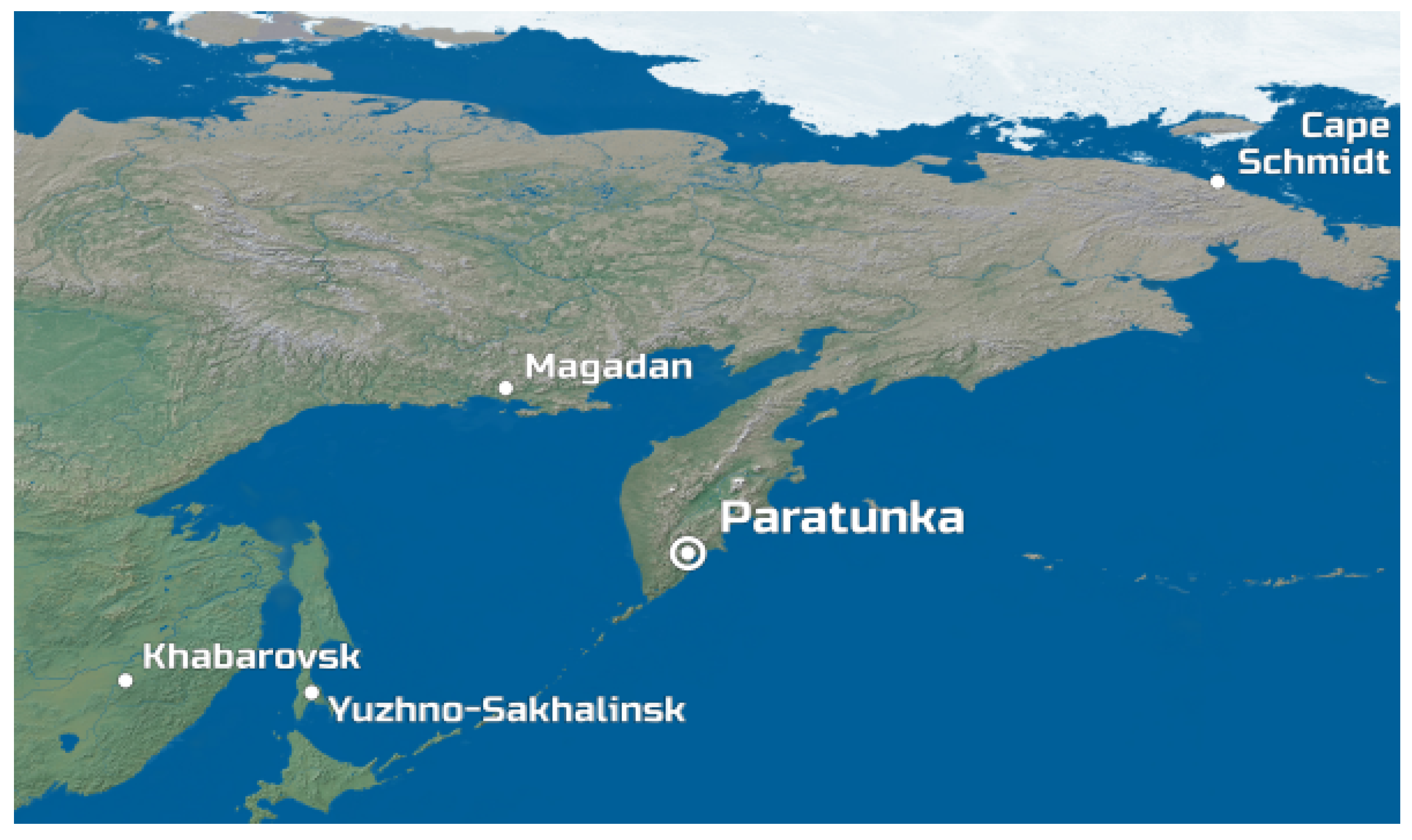
The Paratunka Observatory ($\phi =52.{97}^{\circ }$ N; $\lambda =158.{25}^{\circ }$ E) is located on the Northwest Pacific Ocean on the Kamchatka Peninsula, Russia (Figure 1). The location of the sensor is 10 km from the ocean coast on a flat area. Thunderstorms in Kamchatka are a very rare meteorological phenomenon. Forecasters attribute this phenomenon to the peculiarities of the local climate, which is highly unstable, determined by the influence of the surrounding seas, the constant movement of air masses due to atmospheric pressure drops, and the influence of cyclones coming from the Pacific Ocean. Despite the high cyclonic activity, the average number of thunderstorm days per year on the peninsula, according to Yandex.pogoda, is 10.8. The main specialization of the observatory is fair weather electricity. Continuous observatory observations of the atmospheric electric field began in 1997 and continue to the present. This paper presents the main results for this observation period.

The electric field in the atmosphere, like any electric field, can be determined at any of its points by the value of a scalar quantity called the potential $\phi$. The considered time scales are such that the electric field can be considered potential, thus:

$$\overrightarrow{E}=-\overrightarrow{▽}\phi ,$$

(1)

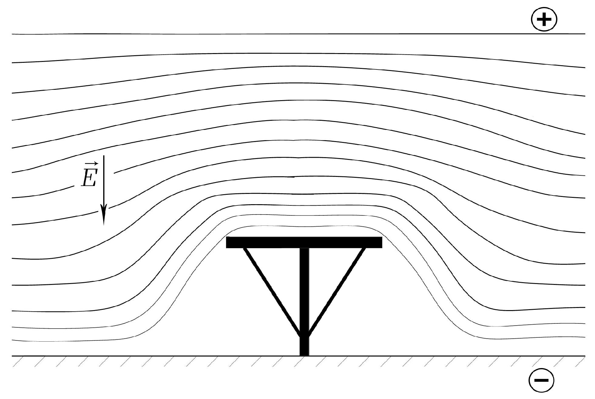
where $\overrightarrow{▽}\phi$ – is the electric field potential gradient (PG). It is known that the earth’s surface is negatively charged, while the ionosphere is positively charged. Under conditions of an undisturbed field, the potential grows with height, the lines of force are directed downward, and we take the direction from the earth’s surface as the positive direction of the normal. Figure 2 conventionally shows the positive charge of the ionosphere, the negative charge of the Earth, the design of the sensor installation, and the level surfaces of the electric field strength in the vicinity of the sensor installation.

A discharge current flows from the ionosphere to the ground. The density of this current j is determined by the formula:

$$j=\lambda E+\rho V+D_t▽\rho +\mathsf{\Sigma }{J}_s,$$

(2)

where $\lambda$ is the electrical conductivity of the atmosphere; E is the electric field strength; $\rho$ is the density of electric charges; V is the hydrodynamic velocity of the medium; $D_t$ is the turbulent diffusion coefficient; and $\mathsf{\Sigma }{J}_s$ is total current density of S sources. The first term is the conduction current in the atmosphere due to the global lightning generator. The second and third terms take into account the local currents in the exchange layer of the atmosphere caused by the convective generator. The last term includes possible sources of both local and global scale. The first of them include cloudiness, precipitation, local lightning discharges, and subsoil radioactive gases. An additional global current source is the effects of space weather.

2. A Set of Tools for Studying the Electrical Characteristics of the Surface Atmosphere

The main instrument for AEF measurements at the Paratunka Observatory is the Pole-2 sensor, developed at the Main Geophysical Observatory Russia. Pole-2 is an electrostatic fluxmeter type device. PG is converted into electric current by means of a rotary electrostatic generator, which is based on the phenomenon of electrostatic induction. The flow of electrostatic induction of the measured field induces an electric charge on the measuring plate. The shielding plate periodically shields the measuring plate in an electric field, due to which the value of the induced charge changes periodically. The charge flowing in and flowing from the plate creates a current in the load circuit. The amplitude of this current is proportional to the PG, the frequency of rotation of the modulating plate and the area of the measuring plate, and the phase is determined by the direction of the electric field at the surface of the measuring plate.

Measurement of PG in the Pole-2 sensor is carried out through two channels. The first channel has a resolution of 0.16 V/m and a dynamic range of $\pm 200$ V/m. The second channel has a resolution of 1.6 V/m and a dynamic range of $\pm 2000$ V/m. When processing the measurements, the readings of both channels were taken into account.

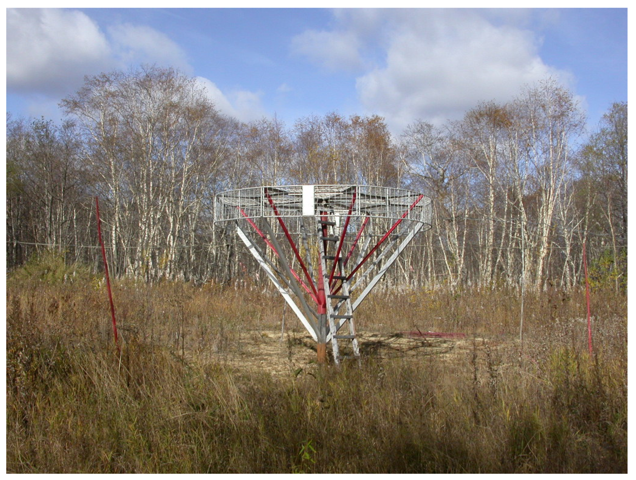
Pole-2 is installed on the site 200 m from the administrative building (Figure 3) at a height of 3 m. The area around it is cleared of trees within a radius of 12 m. The design of the sensor installation is such that the level surfaces of the electric field strength at the measurement point are parallel to the surface land (Figure 2). The lattice design allows air ions to rise freely from the ground surface to the measurement point.

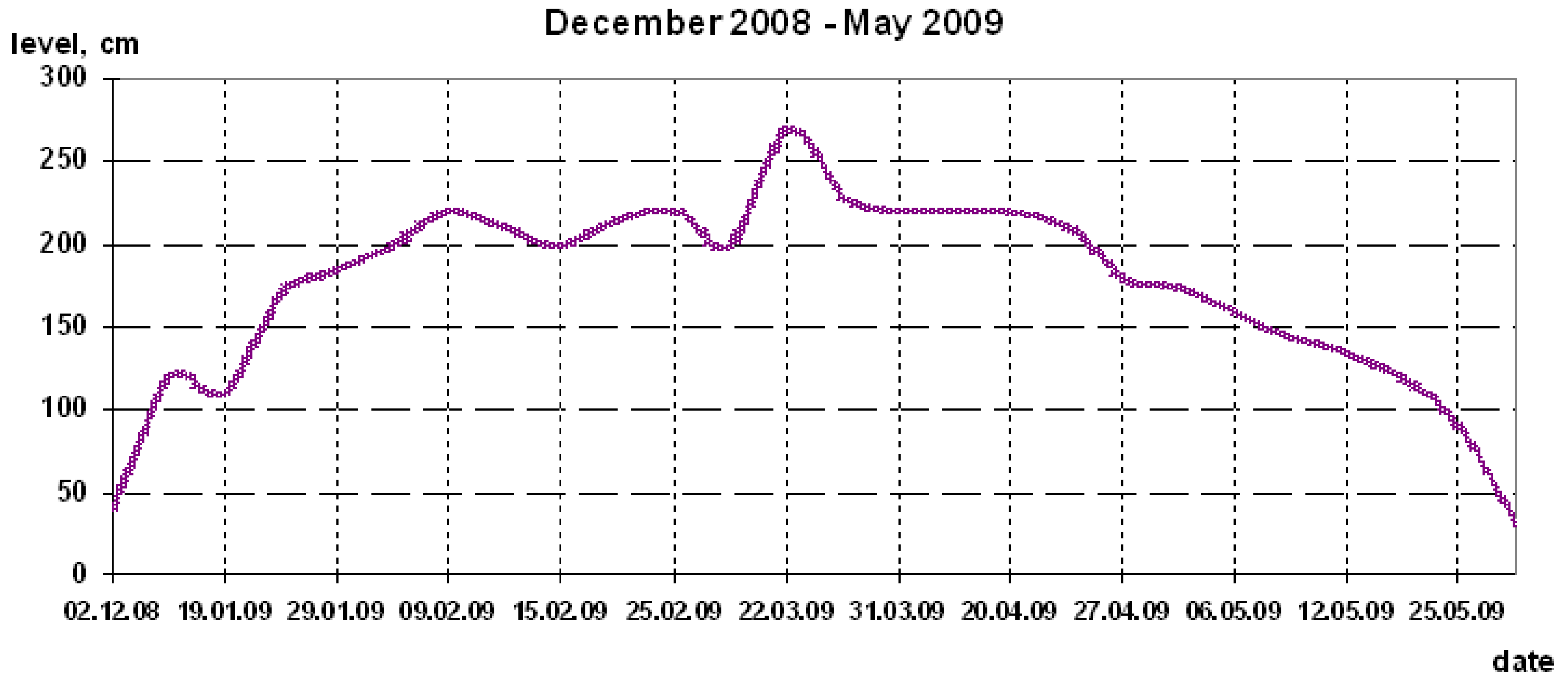
The height of the sensor installation was determined by the maximum snow level in winter. The snow level in winter in the area of electric field measurements reaches 2.7 m (Figure 4).

The next instrument for measuring the electrical characteristics of the atmosphere is “Electrical Conductivity-2”. It was also developed at the Main Geophysical Observatory Russia. The principle of its action is as follows. Air is blown through a pipe, to the walls of which a condenser is attached. Under the influence of a voltage applied between the plates of the capacitor, an electric current flows to the inner plate. The value of this current is proportional to the value of the polar electrical conductivity. Separately, the electrical conductivity of the air, caused by positive ions and separately by negative ones, is measured. The measurement interval is 1 s.

The electrical characteristics of the lower atmosphere are highly dependent on meteorological conditions. Therefore, the instruments of the Paratunka Observatory include a digital weather station. It measures the following parameters: air temperature; humidity; wind speed; direction of the wind; pressure; precipitation level; solar radiation intensity; and solar energy flux density. The measurement interval is 10 min. The researcher keeps a log of observations. Meteorological phenomena, the level of cloudiness, the level of snow in winter (Figure 4), and the phenomenon of fog are recorded there. The rain gauge can only correctly measure liquid precipitation. The phenomenon of snowfall is determined by records in the observation log and by measuring the snow cover.

The measurement results are broadcast on the Internet. At the end of the day UTC charts are built on the page http://www.ikir.ru/en/Data/electr.html (accessed on 12 February 2023). Access to the archive of measurements is provided through the Common Use Center “North-Eastern Heliogeophysical Center” [http://www.ikir.ru/en/CUC/ (accessed on 12 February 2023)].

3. Observed Effects and Main Results

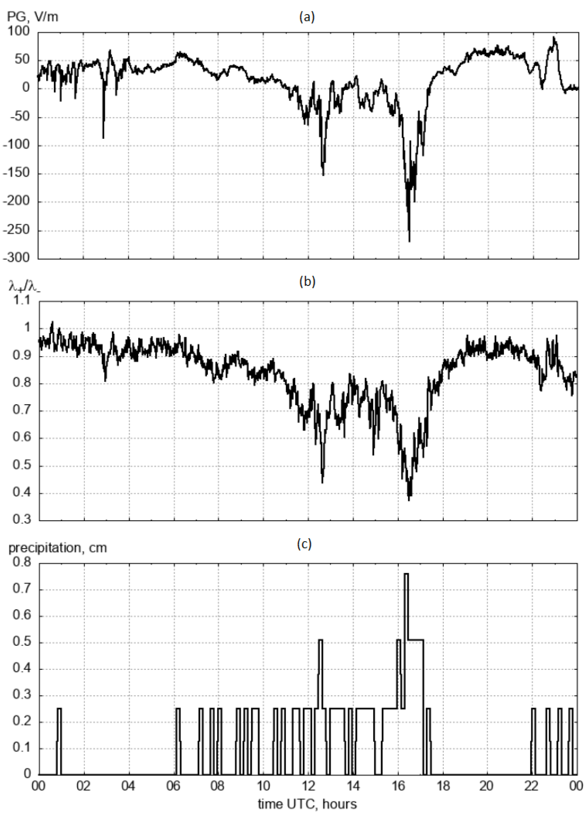
Precipitation influences the AEF measurements the most. To isolate other signals, we need to know how precipitation affects the electrical characteristics of the surface air. Figure 5 shows an example of rain for 8 August 2009. Figure 5a shows the PG curve. On Figure 5b shows the unipolarity curve: air conductivity caused by positive ions divided by air conductivity caused by negative ions. Figure 5c shows the level of precipitation. The rain effect is manifested in a large negative PG bay and unipolarity. The effect of rain from thunderclouds in PG is represented by a high-amplitude alternating signal.

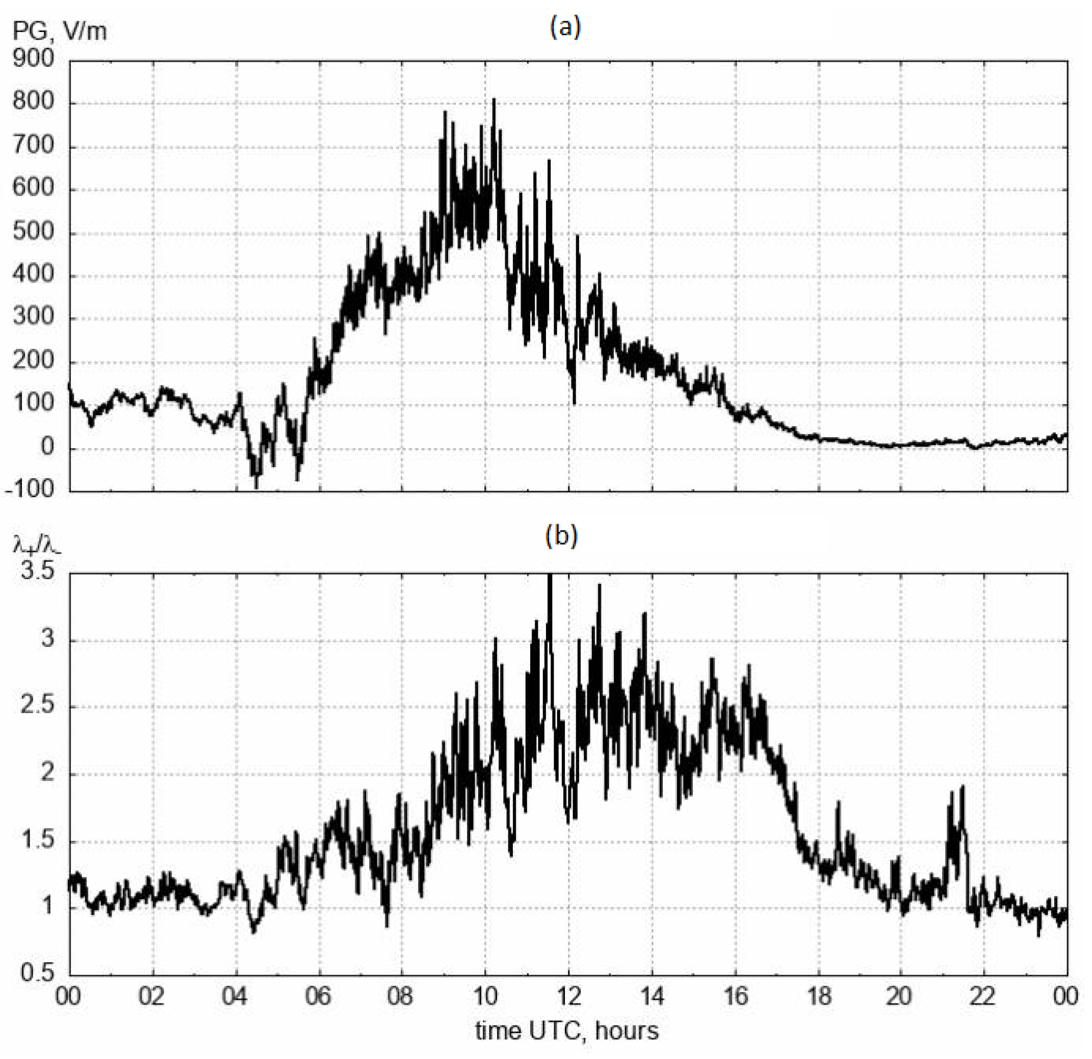
Figure 6 shows the effect of snow in the electrical characteristics of the surface air for 26 February 2010. Figure 6a shows the PG curve. Figure 6b shows the unipolarity curve. The snow effect manifests itself in a large positive bay PG and unipolar electrical conductivity. The rain gauge could not register snow correctly. Therefore, the snow phenomenon was determined from the observation log.

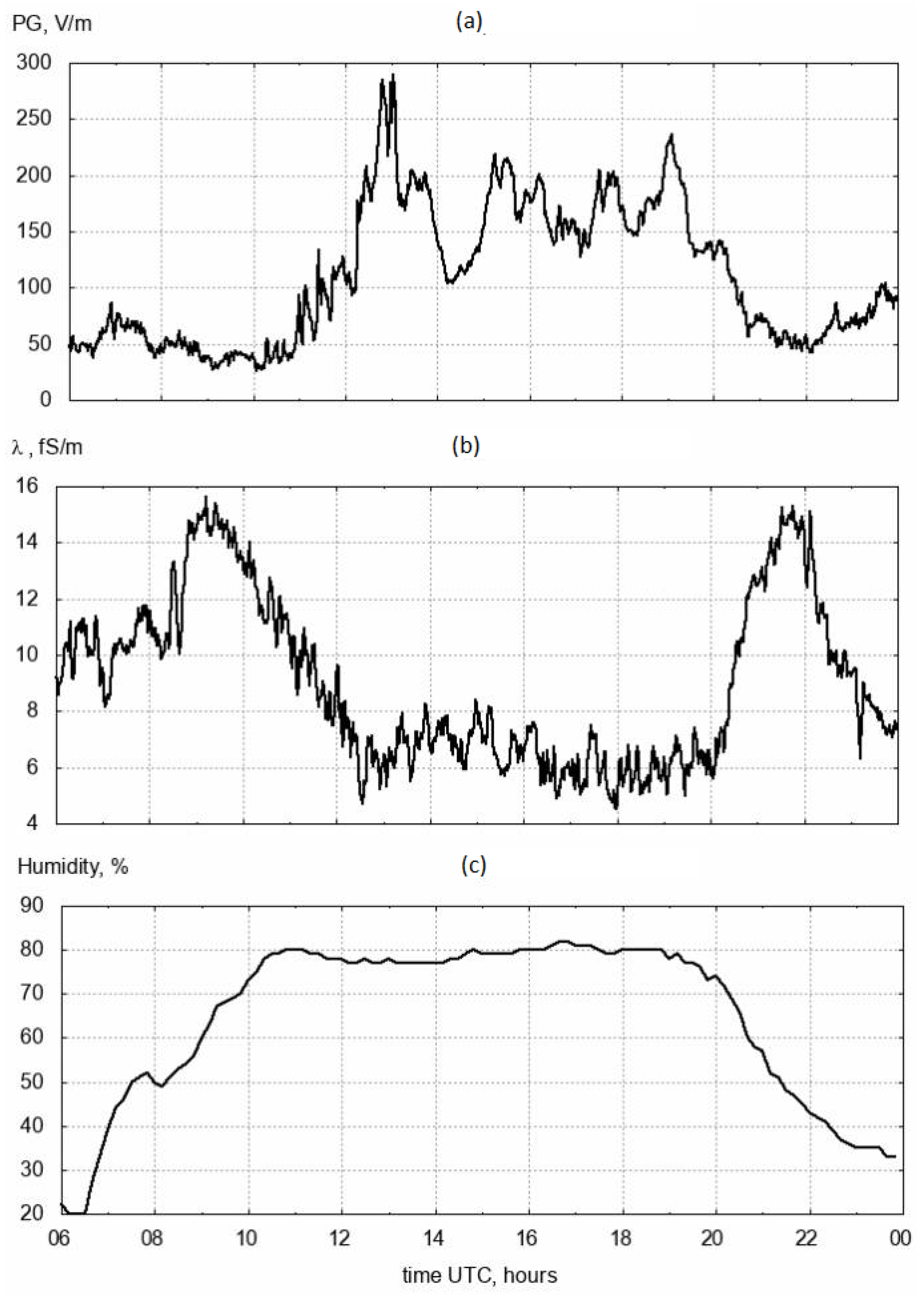
The next meteorological phenomenon that affects PG is fog (Figure 7). It was determined visually by the researcher and recorded in the observation log.

During fog, the average levels of PG (Figure 7a) and air humidity (Figure 7c) increase. The average electrical conductivity of the air decreases during fog (Figure 7b). The electrical conductivity in this case is calculated as the sum of the electrical conductivity caused by positive ions and the electrical conductivity caused by negative ions $\lambda ={\lambda }_{+}+{\lambda }_{-}$.

The explanation for this behavior of PG during fog can be as follows. The electrical conductivity depending on the mobility of ions can be represented by the formula

$$\lambda =e\mathsf{\Sigma }\left(n_i{u}_i\right),$$

(3)

where n is the concentration of particles and u is their mobility.

The mobility of ions is the speed of their movement in an electric field of intensity equal to unity. It is determined in a simplified form by the Langevin formula:

$$u_i=a\frac{e_i}{m_i}\frac{l_i}{v_i},$$

(4)

where a is a certain numerical coefficient, $e/m$ is the ratio of the charge to the mass of the ion, l is the mean free path of the ion, and v is the average speed of its random motion.

The mechanism of behavior of the electrical conductivity of air during fog is as follows. Water molecules attach to the charged ions of aerosols, which sharply reduces their mobility. A decrease in mobility leads to a decrease in electrical conductivity. With a relative constancy of the conduction current, in the case of a decrease in the electrical conductivity of the air, the value of PG increases (Figure 7a).

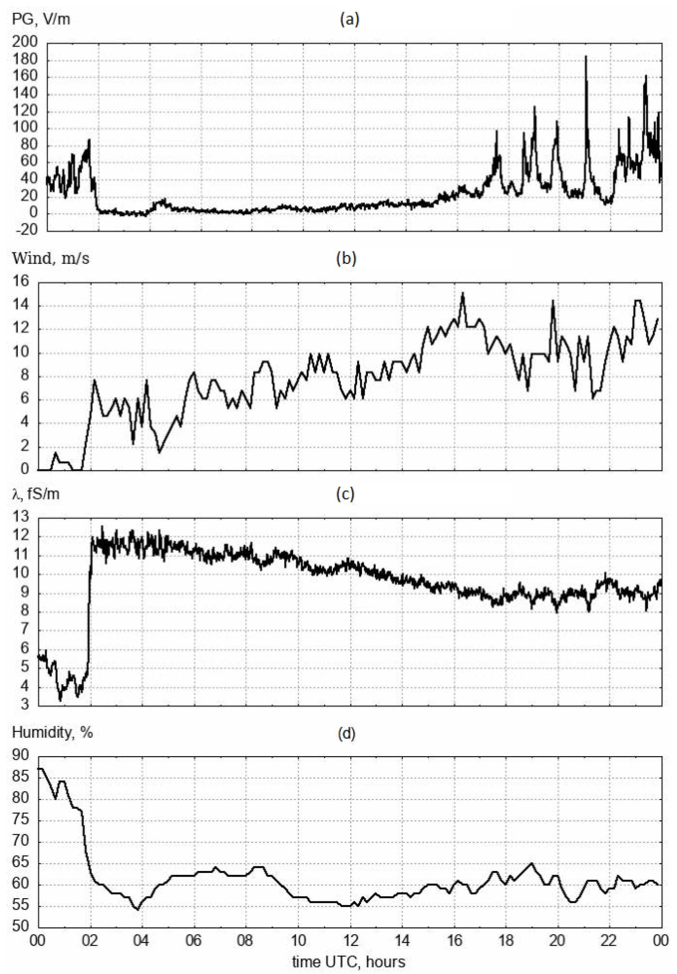
When studying the effect of wind in atmospheric electricity, one should take into account the season, the state of the earth’s surface, and cloud cover. An example of the wind effect in the AEF at the Paratunka observatory in winter for 14 December 2021 is shown in Figure 8. At 2:00 UTC, the wind speed increased (Figure 8b). The flow of dry cold air reduced the humidity of the ground air (Figure 8c). A decrease in air humidity according to Formula (3) leads to an increase in electrical conductivity. An increase in the level of electrical conductivity leads to a decrease in the PG level. After 16h UTC, the wind strength increased (Figure 8b) and the snow begins to blow. Snow particles broke off from the surface of the snow cover, charged, and created large PG fluctuations at the sensor (Figure 8a).

Extensive literature is devoted to the effect of the sunrise in an electric field. A review of early publications was given by Chalmers [10]. PG measurements performed on cloudless days [11] showed its increase by two to three times after sunrise. At the same time, the electrical conductivity of the atmosphere increased by only 20% compared with the corresponding values before sunrise. This effect is explained by the action of a convective generator [12]. In the morning, convective and turbulent processes increase, the second and third terms in Formula (2). This leads to an increase in the electrical conduction current and an increase in PG.

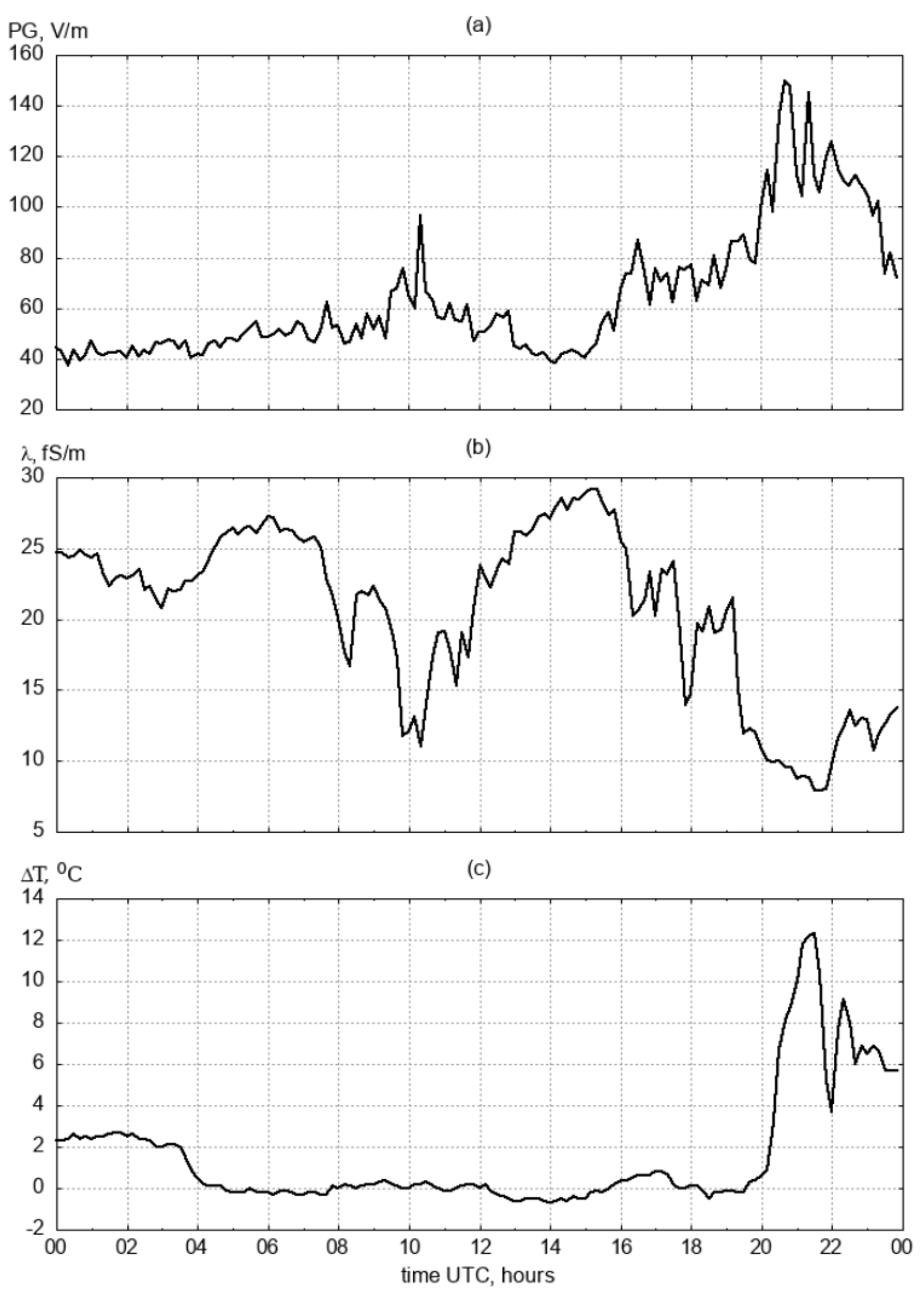
A comparison was made of the main characteristics of the sunrise effect in the diurnal PG variations obtained at Paratunka Observatory with the results of other authors. It turned out to be a good match [13]. An experiment was conducted at the observatory to directly confirm the presence of a convective generator in the global electrical circuit [14]. For this, in addition to PG observations, we used simultaneous records of the electrical conductivity of the atmosphere, as well as its temperature near the earth’s surface and at a height of 25 m (Figure 9). Local time is 12 h ahead of world time, LT = UTC+12. Sunrise began at 20:00 UTC (8:00 LT). At this time, PG increased (Figure 9a). At the same time, the air temperature difference at heights of 3 and 25 m increased (Figure 9c). An increase in the vertical temperature gradient increases convective processes. The electrical conductivity of the air decreased both in the morning and in the evening (Figure 9b). The relationship between PG variations and the temperature difference is most closely manifested at sunrise with a correlation coefficient of ∼$0.6\pm 0.1$ [14]. The appearance of the evening and morning maximum in the daily variation of PG in fair weather conditions does not correlate with meteorological phenomena: humidity, wind strength and direction, precipitation, or cloudiness.

The sunrise effect also manifests itself in the spectral characteristics of the electric field. At sunrise, in the PG power spectra in the surface atmosphere in Kamchatka, an increase in the intensity of oscillations was found in the band of periods of 2–2.5 h [15].

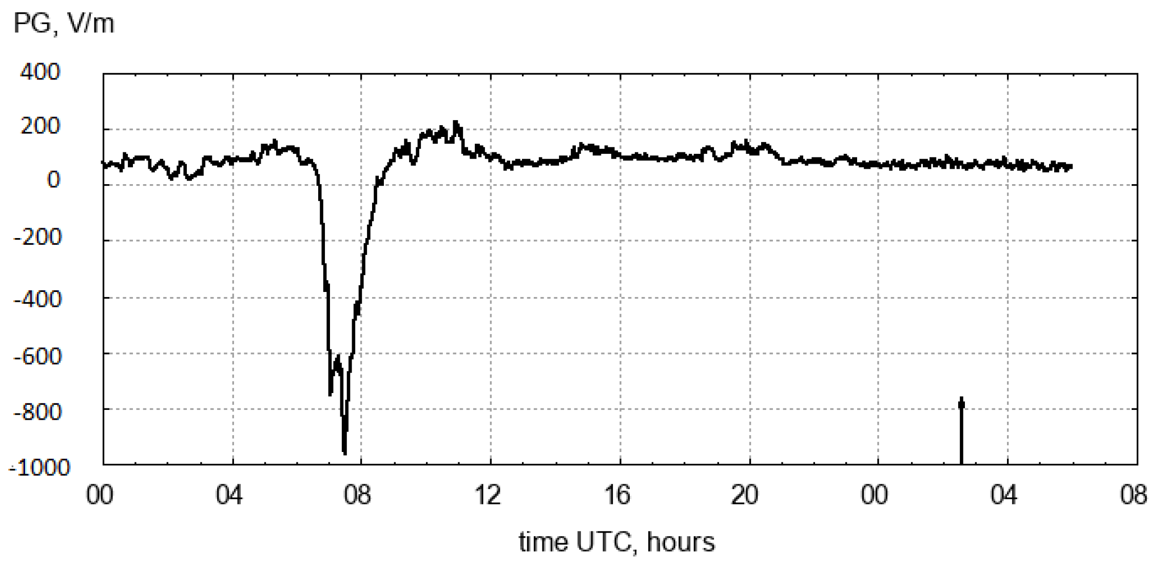
Negative PG anomalies before seismic earthquake (EQ) events are a fairly well-known precursor of earthquakes. Such anomalies began to be determined after the appearance of instruments capable of detecting signs of anomalies in PG. For example, one of the early studies of anomalies before EQ with fixation of the PG sign was done in Japan [16]. A review of publications on this issue was made in [17]. The negative anomaly in PG before the earthquake on 27 July 2022, Ms = 4.5 $\phi =53.{26}^{\circ }$ N; $\lambda =160.{73}^{\circ }$ E, distance 168.2 km is shown in Figure 10.

A statistical analysis was made of the appearance of negative anomalies before earthquakes in fair weather conditions. A seismic event was considered to be a situation when, in the time interval 24 h after the anomaly, one or several EQs of class K from 11 to 15 ($Ms\cong$ 4.7–6.7) occurred with epicenters in the area with coordinates (45–55)${}^{\circ }$ N, (155–165)${}^{\circ }$ E, including registration point PG. For the period from 1 January 1997 to 31 December 2002 (i.e., for 2189 days) 103 cases of anomalous behavior of the PG component were detected. In 37 (36%) cases, earthquakes occurred after the anomaly in 1–24 h [17]. The seismic regime in the specified area during this period was such that the number of random EQs of class higher than 11 would be 19. Thus, the excess over the random value was 37/19 = 1.9 times.

This forecasting method strongly depends on the meteorological situation at the observation point. During rain, snow, fog, strong wind, or overcast, the PG signal is many times higher than the signal from earthquake precursors. The paper evaluates the possibility of predicting earthquakes by negative anomalies of the atmospheric electric field in any weather conditions. Based on continuous observations of the electric field in Kamchatka for the period 1997–2002, the work of this precursor was evaluated. It turned out that the efficiency of this forecasting method under any weather conditions is no more than 10% [18].

Another harbinger of earthquakes is the amplification of atmospheric gravity waves (AGW). Such waves easily pass from the lithosphere to the heights of the ionosphere [19]. Recently, with the development of methods for studying the total electron density in the atmosphere, researchers of lithospheric–atmospheric–ionospheric interactions have begun to pay attention to this [20,21]. 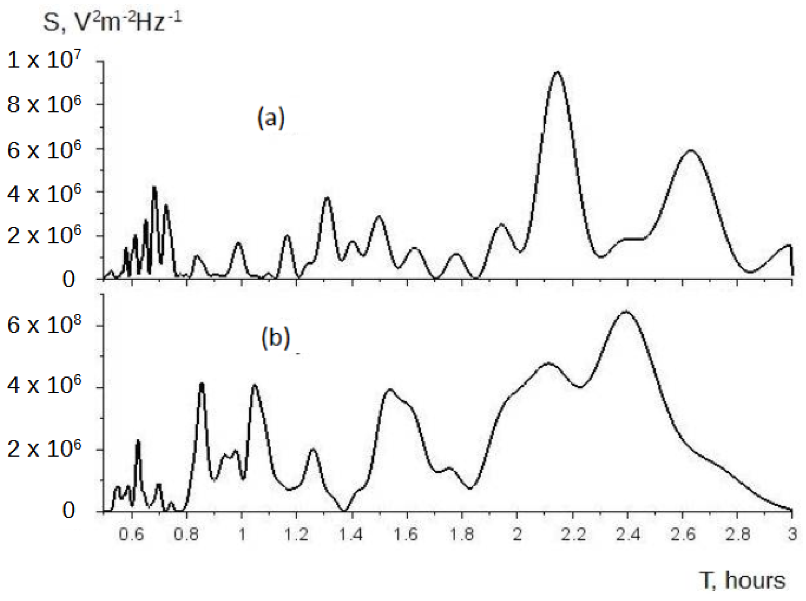Directly in electric field variations, the AGW enhancement during and on the eve of earthquakes was identified at the Paratunka observatory as early as 2004 [22]. It was shown that, on days with earthquakes, the intensity of the power spectra in the range of AGW periods under fair weather conditions increases by an order of magnitude. However, in case of bad weather, this intensity increases by an order of magnitude. A similar effect of AGW amplification in an electric field was observed in Japan [23]. The AGW amplification effect is shown in Figure 11. Under fair weather conditions on 6 November 2007, the PG power spectrum in the range of AGW periods is shown in Figure 11a. In comparison with the AEF of fair weather on 17 September 1999 on the eve of the 18 September 1999 earthquake (Ms = 6.1 $\phi =51.{21}^{\circ }$ N; $\lambda =157.{56}^{\circ }$ E, distance 201.2 km), the intensity of the power spectra increased by an order of magnitude (Figure 11b).

The response of atmospheric electricity in the surface layer of the atmosphere to magnetic storms in fair weather conditions depends on many factors. First of all, one must pay attention to where the observatory is located. The strongest magnetospheric disturbances in the electrical parameters of the surface atmosphere are manifested at high-latitude stations [24,25,26]. This is primarily due to the precipitation of solar wind particles into the atmosphere in the subpolar regions of the Earth. For mid-latitude stations, the relationship between PG and magnetic storms is not so unambiguous. The complex nature of the behavior of PG in a large amount of statistical material (15 cases) was recorded at the Mohe Observatory (China, $53.{482}^{\circ }$ N) [27]. The authors concluded: “At the onset of geomagnetic activity, such as sudden changes of IMF-Bz, the solar wind proton number density, also Ez is typically seen to undergo large changes, but the three have a nonlinear relationship” (here Ez is PG) [27].

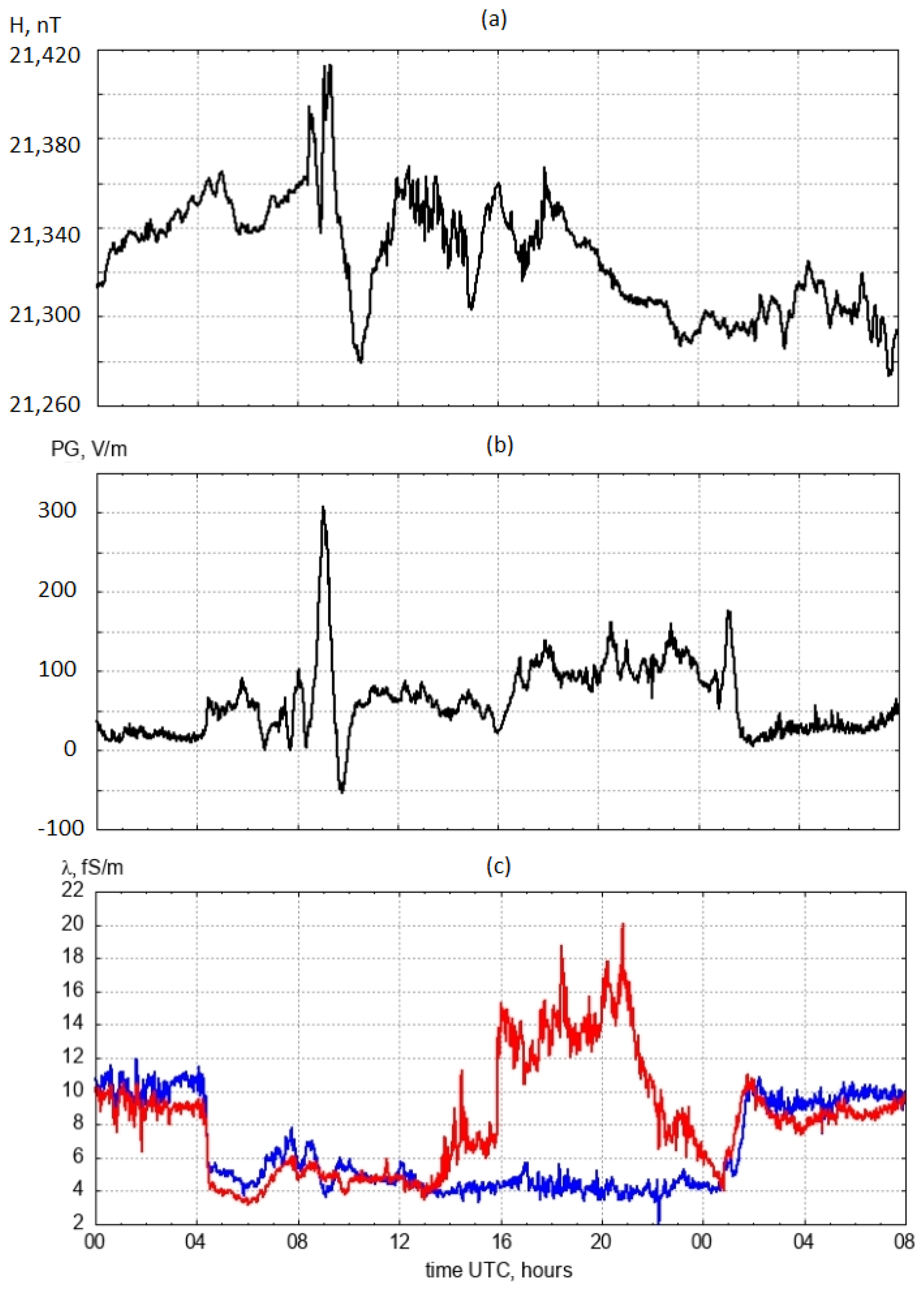
According to the Paratunka Observatory (${52}^{\circ }58.{33}^{\prime }$ N), each magnetic storm has its own character and each storm must be processed separately. The effect of the magnetic storm on 5 April 2010 is shown in Figure 12 [28]. The development of this process in time can be traced from the graph of the H-component of the magnetic field (Figure 12a).

Three effects can be traced in the development of this storm. The first is related to the decrease in the electrical conductivity of the air (Figure 12c). Such a decrease could be due to the “switching off” of one of the ionizers of air molecules. The ionizers at this level are radon and galactic cosmic rays. The seismic situation at that time was calm, which means that there were no significant deformation processes that would lead to a sharp increase in radon emanation. This means that the decrease in electrical conductivity can be associated with a decrease in the flux of galactic cosmic rays.

The second effect manifested itself in sharp changes in PG during the initial stages of the storm (Figure 12b). Apparently, it is connected with the inductive phenomena of electromagnetic processes. What exactly these processes are is not yet clear. It can be assumed that solar cosmic rays can contribute to additional ionization of the upper atmosphere and, thereby, increase the current of the global electrical circuit of the atmosphere. This would lead to a change in the electric field near the earth’s surface. Other mechanisms of this effect cannot be excluded.

The third effect showed an increase in electrical conductivity caused by positive ions (Figure 12c). It is not yet clear whether this effect is caused by meteorological or geophysical processes. This can be found out with more statistical material.

4. Conclusions

The Paratunka Observatory, located on the Kamchatka Peninsula in the Northwest Pacific Ocean, has a number of features for measuring atmospheric electricity. There is very little thunderstorm activity here, so the observatory specializes in field variations in fair weather conditions. The Kamchatka region is characterized by high seismic activity, so it is convenient to study the relationship between atmospheric electricity and earthquakes here. The possibility of predicting earthquakes by negative anomalies of atmospheric electricity in fair weather conditions is shown. This method can be supplemented by detection of the generation of atmospheric gravity waves on the eve of earthquakes. The Paratunka Observatory is a mid-latitude observatory and this must be taken into account when studying the effect of solar activity on the lower atmosphere of mid-latitudes. The observatory is open for contacts with the international scientific community.