Analysis and Visualization of Production Bottlenecks as Part of a Digital Twin in Industrial IoT

Abstract

In the area of industrial Internet of Things (IIoT), digital twins (DTs) are a powerful means for process improvement. In this paper the concept of a DT is explained and analysis possibilities throughout the life-cycle of a product and its production system are explored. The main part of this paper is focused on an approach to the analysis of manufacturing layouts and their parameters. The approach, which is based on a state of the art bottleneck detection method, allows an intelligent representation of the temporal process characteristics. The presented method is widely applicable for any type of manufacturing layout and time-span. The use of elementary heuristics leads to traceable results that can be used for further analysis or optimization. The results of this analysis method can be integrated in a DT and combined with machine learning and explainable artificial intelligence (XAI). The concept for a self-learning DT is explained and implementation possibilities are elucidated.

1. Introduction

Over the past years, the areas of more efficient production, smart manufacturing and Internet of Things (IoT) have been emerging faster and faster. The well known term IoT describes a vast array of entities with sensing and actuating capabilities that collect, analyze and share data across other entities, programs and platforms and influence the state of other entities [1]. A common definition of industrial IoT is proposed by Ben-Daya et al. [2]: “Internet of Things is a network of physical objects that are digitally connected to sense, monitor and interact within a company and between the company and its supply chain enabling agility, visibility, tracking and information sharing to facilitate timely planning, control and coordination of the supply chain processes". Integration of IoT in manufacturing is known as Industrial IoT (IIoT). In the scope of IIoT, the application of digital twins (DTs) is receiving enormous attention. Many researchers consider DTs as the most promising current trend in the scope of product development, production design and operations management [3,4]. By means of the application of DTs, engineers in product development may benefit from the vast amount of information gathered in production processes and in product operation [5]. The main elements of DTs are integrated multi-physics, multi-scale, deterministic and probabilistic simulations of a complex technical system; they use the best available analytical models in combination with continuously updated sensor readings to mirror the state of its corresponding physical twin [4]. Meanwhile, a general consensus can be observed that a DT consists of three parts: physical product or system, virtual representation and connected data that tie these products or systems together [4]. Trauer et al. [6] list three key characteristics of DTs:

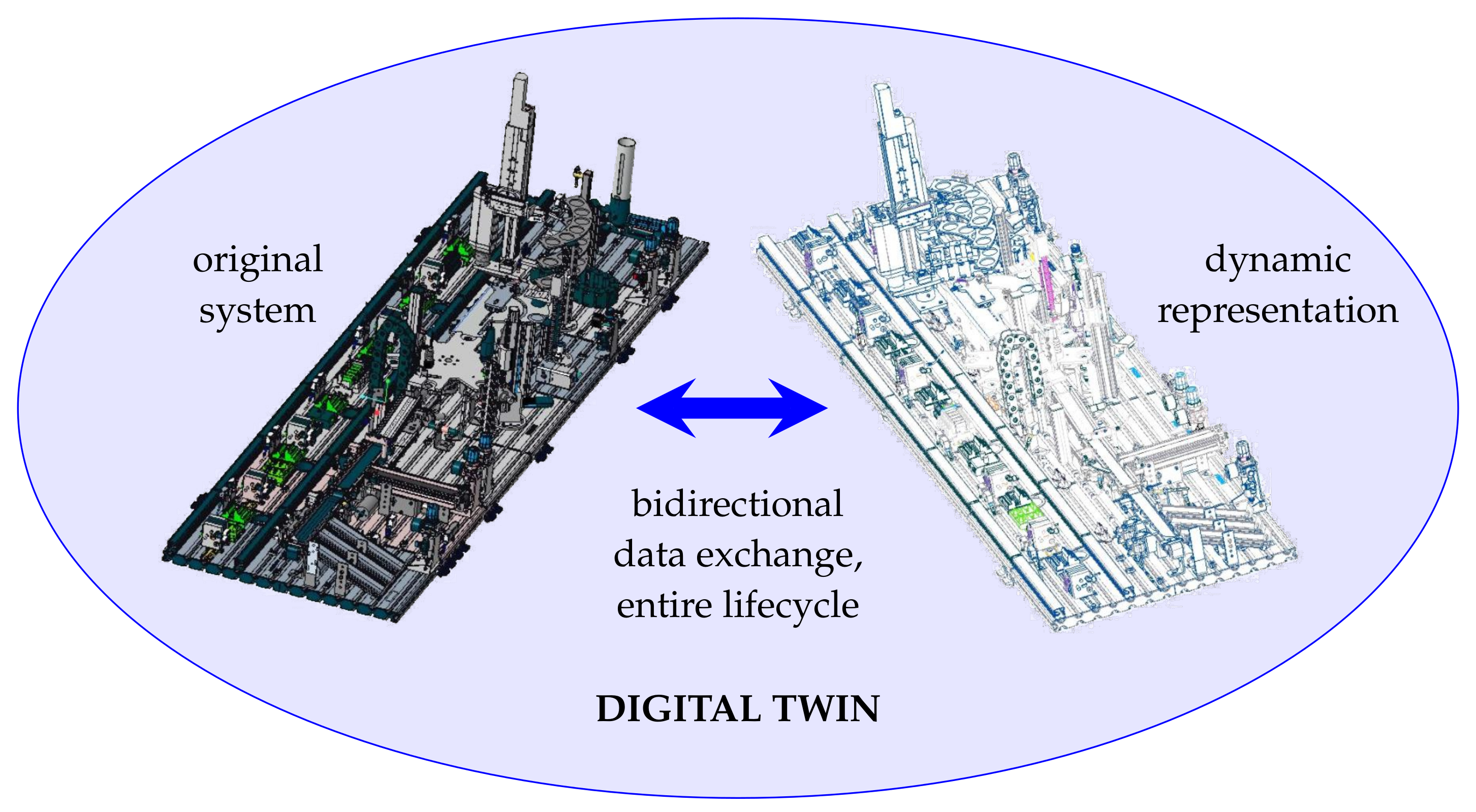
• DTs are dynamic virtual representations of real technical systems;
• DTs are connected to the real technical system over the entire life-cycle;
• Data are exchanged bidirectionally between DTs and the real technical system.

The main characteristics of DTs are summarized in Figure 1.

Whereas the first characteristic is obvious, the second requires closer examination. A life-cycle of a product and its production system is shown in Figure 2.

Both the development cycle of the product itself and of the production system are shown in form of a V-model, which is the common process description model in model-based systems engineering (MBSE) and is, for instance, proposed in the VDI guideline 2206 [7,8,9]. This process continues with the production operation and leads to product delivery, product operation and product recycling; this also highlights the potential and necessity of a circular economy. A large amount of research covers the production operation stage and international standards such as the ISO 23247 [10] are already established. Other areas of the product and production life-cycle are not as intensively researched, but they may be very important and are thus also depicted in Figure 2. It is important to note that this kind of holistic view on the product life-cycle is necessary to explore all connection possibilities between a DT and the real technical system (product and production system). It is important to note that early application possibilities of DTs already cover the development of the functional and logical architecture of a product. Engineers need to define the main functions of the new product and are required to deal with various kinds of data (e.g., customer satisfaction surveys, product sales and product competitiveness analyses, etc.) [4]. The amount of data exchanged between the real system and the DT is both huge and scattered. By means of applying a DT that integrates all kinds of data in the physical space of the product, the engineers can gain an understanding of possible product improvements [11]. This also underlines the importance of the third key characteristic: the bidirectional data exchange. The new system can be improved making use of the feedback from customers and the problems in product operation. Similarly, in later phases, the analysis and integration of data is of paramount importance in order to improve production. There are a lot of possible ways to improve production lines to produce items more intelligently and more quickly. A few examples are shop floor routing, avoidance of task delay and the optimization of setup times. Simplifying this very complex problem is one of the most important factors in terms of efficiency. A key factor in smart manufacturing is the throughput. Machines are principally responsible for throughput and are the first elements which come to mind when thinking about improving this parameter. The machine which has the biggest impact on limiting the speed of production is known as a bottleneck machine. This knowledge is of great interest for manufacturing engineers and enables one to increase throughput by improving this worst element. At the beginning of this century, Roser et al. [12] presented the idea of the Active Period Method. This method uses active and inactive time periods of production systems to determine the overall bottleneck. The goal of this paper is a combination of a deeper investigation of the Active Period Method, an investigation of real life industrial data sets, a systematic consideration of crucial aspects and a sensible application of this method to real life data. Furthermore, the objective is the development of a heatmap visualization, serving as input to the optimization of the overall production line. Finally, the presented approaches are embedded into an overall concept of a self-learning DT. Consequently, the paper is structured in the following manner. Section 2 reports the results of an in-depth literature review. Based on these results, the Active Period Method is discussed and validated in Section 3. An appropriate visualization technique for the results of this method is presented in Section 4. Based on the application to real life data, Section 5 explains the concept of a self-learning DT. The paper concludes with a summary of results and an outlook to future research activities.

2. Literature Review

In this section, past research efforts at identifying and predicting bottlenecks within an overall production system are presented (

Table 1. Literature review on existing bottleneck detection methods.

Input	Output	Bottleneck Detection Method
Time series data of active periods	Estimation of Sole and Shifting Bottleneck machines relative to observation period	Active Period Method [13]
Time series data of blockage and starvation of machines	Identification of bottlenecks through starvation of downstream machines and blockage of upstream machines	Turning Point Method [14]
Time series data of active periods	Average of active periods for each machine	Average Active Period Method [12]
Observations of process, inventory states	Ranking of bottleneck sets	Shop Floor Bottleneck Detection [15]
Arrival of Jobs	Identification of bottleneck machine pools through reinforcement learning	MINERVA: A Reinforcement Learning-based Technique [16]

).

2.1. Bottleneck Detection in Manufacturing Systems

In 2001, ref. [12] came up with a practical bottleneck detection method which uses the active periods of machines, the Average Active Period Method. The active periods of machines are all periods in which a machine is not starved or blocked by surrounding machines. Starvation means that a machine is unable to produce parts due to lacking incoming parts to be processed. A machine is blocked if it cannot start processing because the current workpiece is finished but has not been removed from the machine. A machine is in an active state even if it has broken down or is being equipped, because it could produce if the technical issues would be solved. When applied to shop-floor data, a set of active periods can be calculated. An example for transforming the series of states of a process into a set of active periods is shown in Figure 3.

The next step is to calculate the mean and standard deviation over all active periods for each machine in the set of machines

$$A_i=\{a_{i,1},a_{i,2},a_{i,3},...,a_{i,n}\}.$$

A visualization of this method can be seen in Figure 4.

The process in the graph above is active for 1.500 s on average before being interrupted by a starved or blocked process. This is by far the longest Average Active Period in the system. All other processes reach much shorter Average Active Periods in the graph, being active for only one or two process cycles before interruption.

In 2004, ref. [13] came up with a new bottleneck detection method which also uses the active periods of machines, called the Active Period Method. The idea behind this method is that the longer a process is running without interruption by starvation or blockage, the more likely it is the bottleneck. The two fundamental rules of this method are:

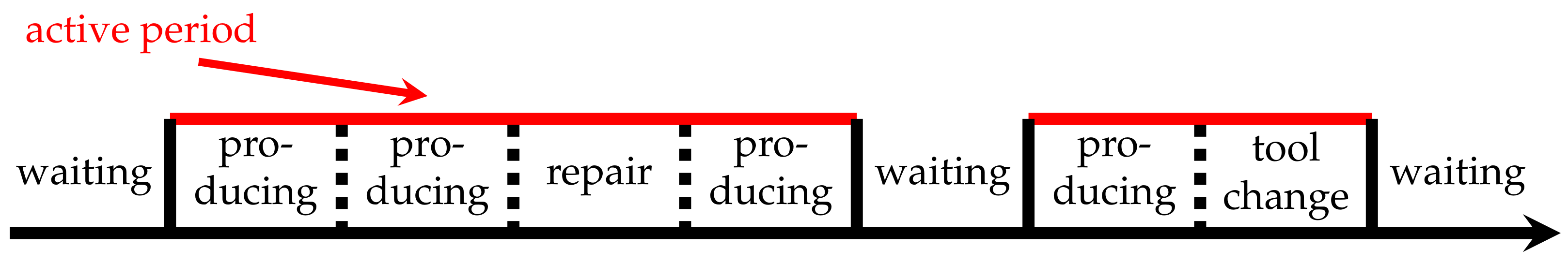
• At any given moment, the process with the longest uninterrupted active period is the bottleneck.
• During the overlap at the end of the current longest uninterrupted active period and the next one, the bottleneck shifts from one process to another.

A visualization of the method described in Algorithm 1 is shown in Figure 5. The figure displays the active/inactive periods of the machines. The upper part of the diagram shows the bottleneck scores for each machine. The bottleneck score measures the ratio between the duration of a machine being a bottleneck and the total observation time of the analysis.

Algorithm 1: Algorithm for the Active Period Method

Input: time series of active periods

Output: list of bottlenecks

1: sort list by starting times

2: for $eachstartingtime$ do

3:   if $firstrun$ then

4:     pick entry with longest duration, add to $bn\_list$

5:     update $last\_bn\_duration$, $last\_bn\_end$

6:   else

7:     pick entry with longest duration

8:     if $endofentryisafterlast\_bn\_end$ then

9:         add to $bn\_list$

10:        update $last\_bn\_duration$, $last\_bn\_end$

11:     else if $startofentryisafterlast\_bn\_end$ then

12:        add to $bn\_list$

13:        update $last\_bn\_duration$, $last\_bn\_end$

14:     end if

15:   end if

16: end for

17: return $bn\_list$

In contrast to the Active Period Method, the Turning Point Method, presented by [14], observes the shift from blockage to starvation. The duration of blockage and starvation are accumulated separately for each machine and set into relation to the observation period. If a machine is a bottleneck, the upstream machines will have a high blockage percentage and the downstream machines will have a high starvation percentage. The bottleneck machine, however, will have low values for both blockage and starvation. Thus, by analyzing the values with respect to the neighbouring machines, one can determine a bottleneck machine. Figure 6 shows an example. Here, machine M3 is the bottleneck, as it is the turning point for the ratio of blockage and starvation percentages.

Another method of determining bottleneck machines is suggested in [15], proposing a walk through the manufacturing layout. This method also uses blockage and starvation periods of machines. When there are machines which are starved, the bottleneck has to be upstream, which means it is somewhere in a process before the starved machines. If there are blocked machines, the bottleneck has to be downstream; thus, it occurs in some later processes. During a walk through the production site, all streams are marked whether the bottleneck is up- or downstream, leading to a set of one or more bottleneck machines. Ref. [16] presented Minerva is a reinforcement learning-based technique, footing on the arrival of jobs coming from the ERP program, which are assigned to machine pools. This method determines a pool of machines as bottlenecks indirectly by maximizing the throughput of the system by an optimal job scheduling. This leads to a machine pool whose capacity needs to be expanded and therefore is a bottleneck pool.

2.2. Evaluation of Bottleneck Detection Methods

In this section the advantages and disadvantages of each bottleneck detection method are discussed. An important aspect is the metric offered by the bottleneck detection algorithms. Whereas [15,16] just identify a set of machines that are bottlenecks, the other methods [12,14] offer a metric that measures how likely a machine is a bottleneck. The metric of the Average Active Period is the average duration of the active periods for each machine. The Active Period Method measures the duration of a machine being a bottleneck. This value is further split into the sole and shifting fraction and then returned as a percentage of the total operation time. The Turning Point Method measures the percentage of starvation and blockage times of each machine. The Average Active Period Method is easy to implement, but does not offer detailed information on the identified bottlenecks. In contrast, the Active Period Method as well as the Turning Point Method offer more accurate metrics with more information on identified bottlenecks.

It is important to note that over the last two decades many approaches and algorithms were proposed for the sensible application of bottleneck detection methods. A conclusive approach for bottleneck detection was proposed in 2008 by Sengupta et al. [17]. Subramaniyan et al. [18] present a data driven algorithm to predict throughput bottlenecks; Roser et al. [19] enhance an algorithm for including the detection of shifting bottlenecks; both are based on the Active Period Method. The application in a simulation software is explored by Leporis and Králová [20]; they also investigated the Active Period Method and identified several advantages.

Another aspect that should be highlighted is the availability of a quality metric, e.g., the accuracy. For the methods from [12,14], no statement on the accuracy is given, while the Minerva method provides an accuracy, e.g., an accuracy of over 90% is reached by [18]. The bottleneck detection method provided in [15] was tested in 20 different production lines and a lot of bottlenecks not considered by experts before were identified.

Although some of the above methods cannot deliver a statement on their accuracy, a big advantage is that they are real-time capable and are easily implemented. The following quality criteria were decisive when choosing the method to be applied:

• Independent of production layout;
• Requires time series data only;
• Implementable in a small prototype;
• Delivers an interpretable metric.

The Active Period Method fulfils all these requirements and is therefore chosen for the proposed bottleneck detection method.

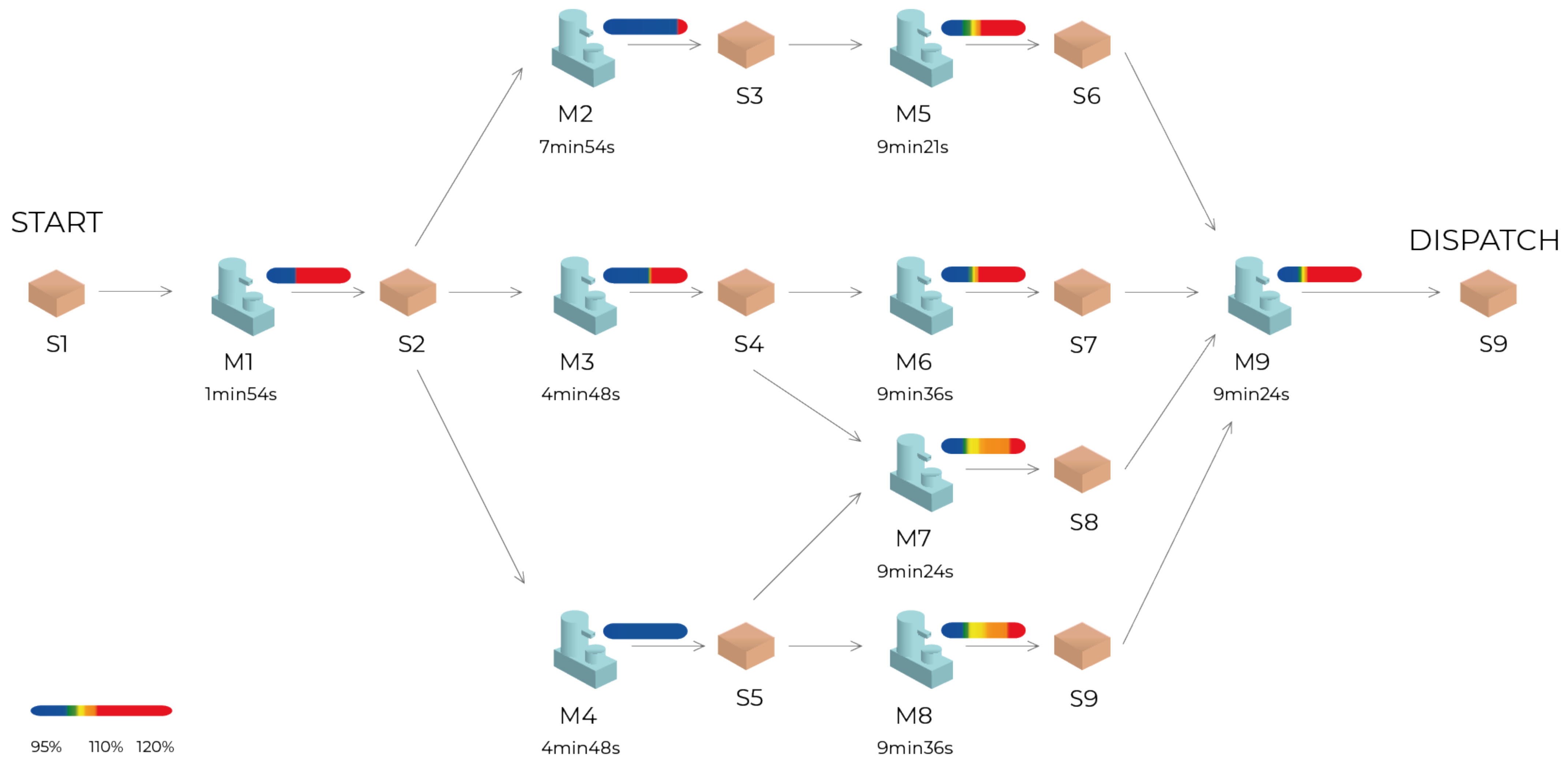
3. Bottleneck Detection Method by the Active Period Method

In this section, the Active Period Method is discussed and validated. The unique research contribution is the combination of a deep investigation of the method, an investigation of real life industrial data sets, a systematic consideration of three crucial aspects and a sensible application of this method to real life data. For this purpose, time series data for operating states from several industrial companies were acquired and analyzed. Subsequently, results were presented to shop floor experts of each company to access the acceptance and practical applicability of the method.

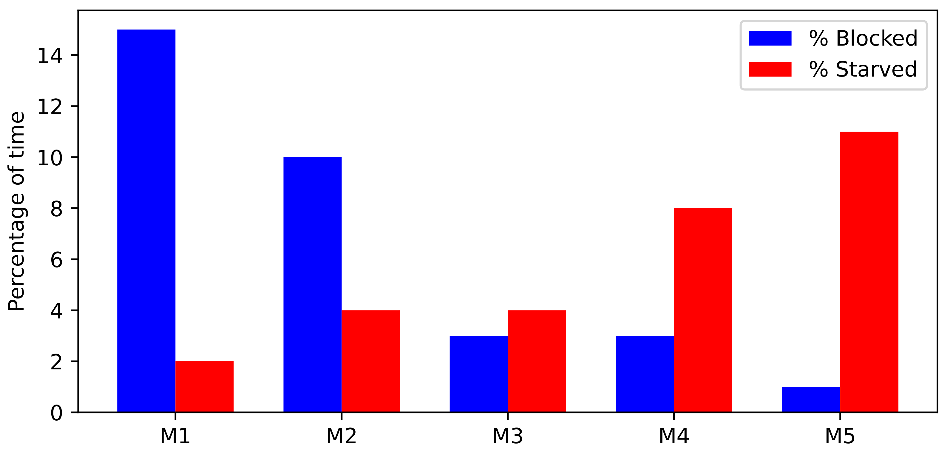
3.1. Boundaries of Active Period Method

To obtain the mandatory information for calculating the Active Period Method, the time series of operating states from the different machines of the overall production system or line is necessary. These data then have to be converted into active periods. Preprocessing the raw time series data is crucial; here, as in smart manufacturing a lot of data are gathered, but the available data are typically not ready for further processing. Assuming that most of the industrial companies use some kind of ERP or PPS software, the following aspects are important in order to apply the Active Period Method:

• Correct interpretation of the operating states. Often, operating states are not recorded correctly. As an example, concrete failure states are often not detected by the system automatically but entered manually at the end of a shift. These errors have to be corrected during preprocessing, which is a time-consuming task.
• Usage of the job schedule. In case of a task change, it is important to set the operating state to free capacity in case the next task does not start immediately. Unsubstantiated downtimes need to be investigated.
• Understanding of the production process. Without any understanding of the product profile, the production layout and structure or special features of the production process, the results of the Active Period Method can hardly be understood.

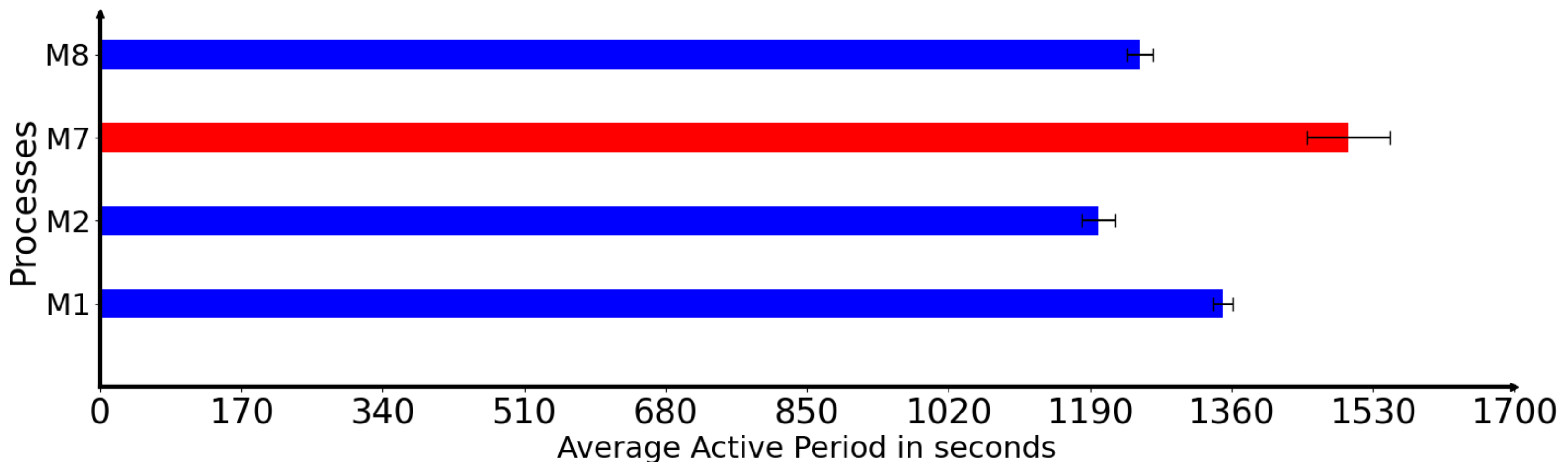
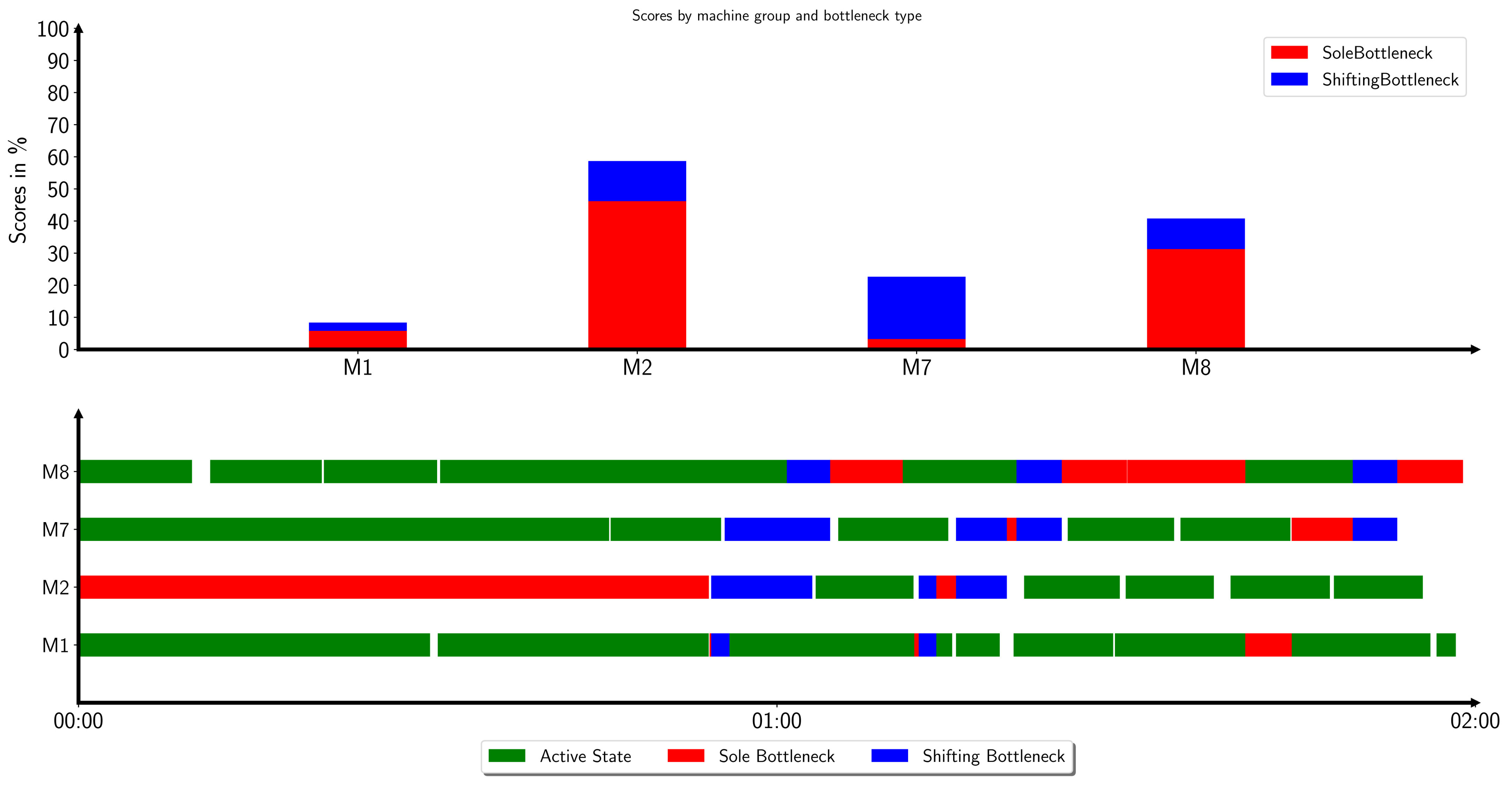
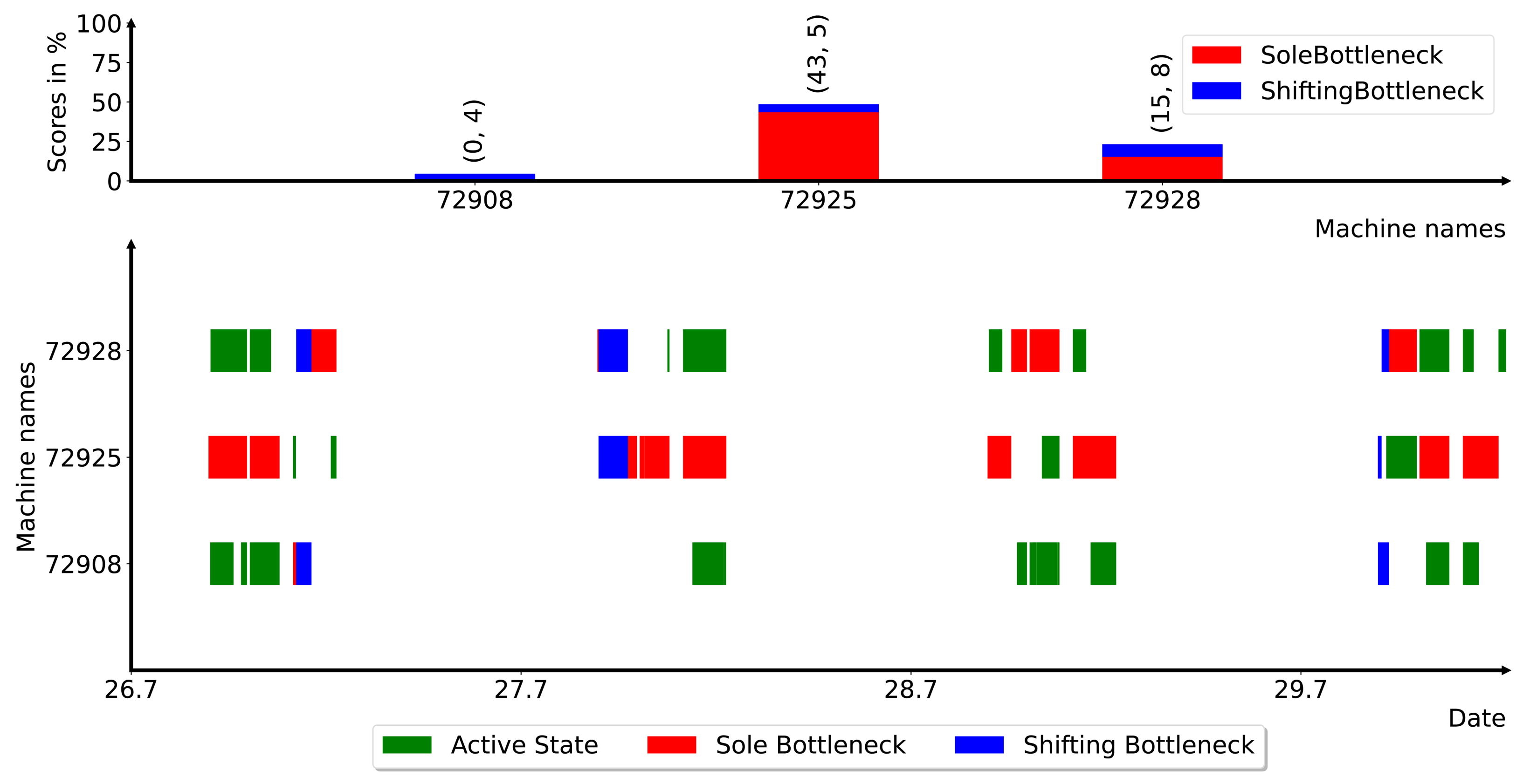
The Active Period Method works with almost any time series data, but as stated above, sufficient knowledge on the production process is important, in order to avoid the misinterpretation of results. In general, the Active Period Method tells which machines are likely to be a bottleneck, not which machines are guaranteed to cause a problem and, thus, false positive results are an issue.

3.2. Results

In Figure 7, an example of the results of the Active Period Method is shown, based on the real production data of one of the industry companies. The graphic shows the data from three different machines, 72908, 72925, 72928. These machines operated for four days. It is clearly shown that machine number 72925 has the highest bottleneck scores, both sole and shifting bottlenecks and, thus, should be examined first when trying to improve the overall efficiency of the production system.

The results were discussed with local experts familiar with the whole production system. The feedback can be summarized as follows:

• General result. The Active Period Method is an appropriate approach to supervise and measure the overall management of a production system. In addition to the sole/shifting bottleneck probabilities, the time series of active and inactive states constitutes a valuable input for production management. Together, these two results provide meaningful and expressive information to judge production quality. In general, the results mirror the experts’ personal opinion and experience on the production system.
• Expressiveness of results and visualizations. The results and presented visualizations are judged as expressive and a good foundation for discussions of potential production system improvements.
• Selection of relevant machines. It should be evaluated whether it is always the best solution to use all available machines as input to the Active Period Method, or if it is better to use an appropriately defined subset instead.
• Observation period. Different observation periods may well affect the results and the quality of the bottleneck prediction of the Active Period Method.

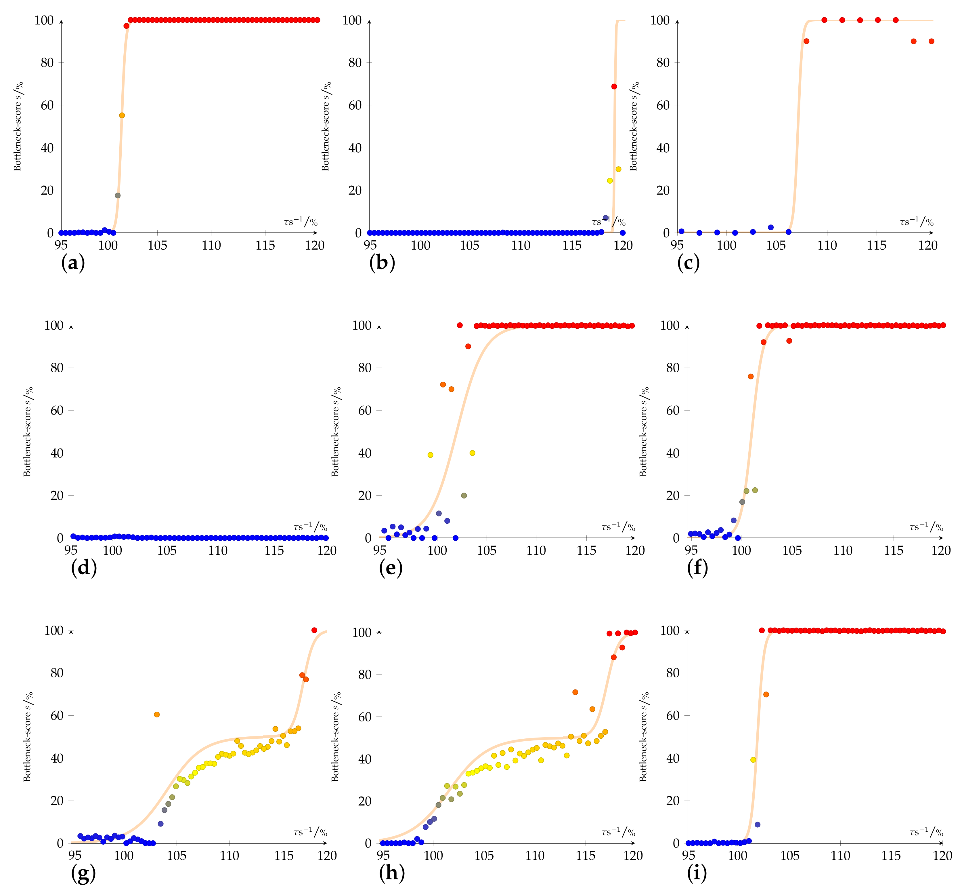
4. Process Heatmap

The Active Period Method identifies potential bottlenecks and offers a corresponding visualization for each machine. In this paper, we introduce a process heatmap as additional analysis and visualization technique, displaying the overall production process topology and the stability of the state of each machine, i.e., how likely the machine might turn into a bottleneck when adapting the overall process topology. Thus, the process heatmap will enable one to judge the health of the production system at once.

The basis for generating a process heatmap is the Active Period Method, because its metric shows a strong tendency concerning which machine is closest to becoming a bottleneck in the manufacturing line. In addition there are no boundaries in relation to physical layouts, so a lot of machine pools or manufacturing layouts can be regarded in different observation periods.

For further investigation, a tangible manufacturing layout given from a planned production line for a certain product is simulated, to demonstrate and validate the process heatmap as intelligent analysis and visualization approach. To simulate the dynamics of the overall production system, a simple model of storage and resistor components is introduced and all kinds of disturbances are modelled by a Gauss distribution. The cycle times of the machines are adopted from the planned production line.

In a first step, the simulation loops over all machines and varies the cycle time from 95 to 120 percent of the calculated mean cycle time for each machine separately as shown in Figure 8. Thus, the cycle times of all other machines are not changed. The density function of the machine cycle times—if a Gauss distribution is used it would be the standard deviation—can be estimated empirically from smart manufacturing data.

The cycle time for each machine is varied in 60 steps and for each step the bottleneck scores are calculated with the Active Period Method. The results are then plotted in a diagram as shown in Figure 8. For visualization purposes, a sigmoid function in the form of Equation (1) is plotted additionally, to show the correlation of this function with the calculated data.

$$f\left(x\right)=\frac{L}{1+e^{-k(x-x_0)}}$$

(1)

Thereby L denotes the limiting value, k is the gradient of the sigmoid and $x_0$ defines the turning point. The variable x describes the average cycle time of the machine in seconds. For a better visualization of these data, the calculated points of the scatter plot are summarised into a color bar. The color bar groups together percentage ranges of bottleneck likelihoods (

Table 2. Color bars for percentage ranges of bottleneck likelihoods.

Percentage	Color
0–20	blue
20–40	green
40–60	yellow
60–80	orange
80–00	red

), so that it is clearly visible how far a machine is from being a bottleneck. The color coding in Figure 8 is the same as described in Table 2. In this figure, it can been seen that, if a machine has wide blue and green areas, it means that decreasing the machine’s throughput, e.g., by slowing down the machine, will not increase its bottleneck score significantly. Machine M4, for example, has a Bottleneck Score of nearly zero throughout the range of $95\%$ to $120\%$, whereas machine M1 quickly changes at $101\%$. This displays that, if a machine has only small blue and green areas, the bottleneck score will increase immediately if the machine’s throughput decreases. Combining the colorbar with the production line layout leads to the results shown in Figure 9. The data displayed in Figure 8 also underly Figure 9.

If each machine of a production system has shifting bottlenecks only and these bottlenecks are evenly distributed, the observed production system is optimally balanced. Having solely shifting bottlenecks within a production system implies that there is no machine which is mainly responsible for being a bottleneck, which leads to a heatmap where the sole bottleneck score is zero at 100% mean cycle time. When trying to optimize a non-optimal production system, the approach is to improve the throughput of the worst machine until it has no sole bottleneck likelihood. When applying this approach to all machines one after the other, the system is optimally balanced and the throughput optimized.

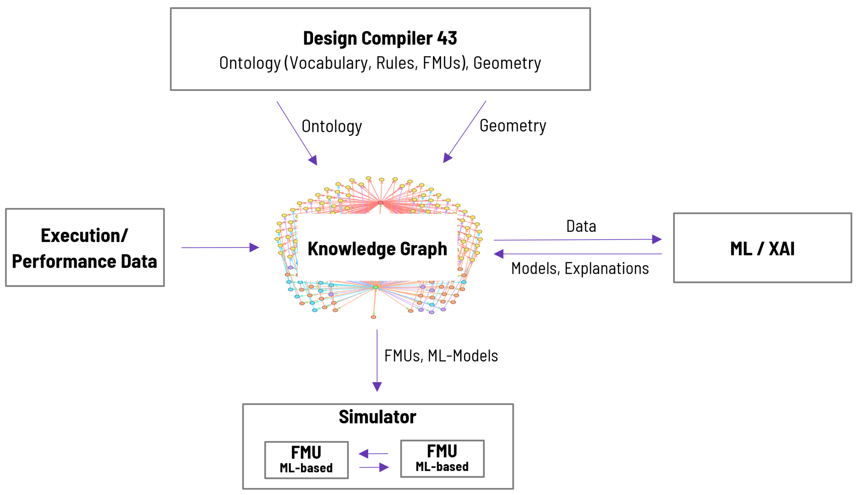
5. Integration of Analysis Results into a Digital Twin

The bottleneck analysis, presented in the last section, analyzes the criticality of each machine within an overall production system and enables the optimization of the production system layout and performance. On a wider scale, such a bottleneck analysis can now be used as part of a dynamic simulation of a production system in the form of a digital twin (DT). Hereby, the bottleneck analysis can be improved by using the DT as a much more precise system model. This way, the cycle times of machines can be considered depending on different process parameters. Compared to the bottleneck analysis approach described in the last section, the behavior of a concrete machine is now not simply defined based on pre-assumptions on its performance under certain conditions, but is deduced from real system behavior based on applying machine learning algorithms on past system execution data. As a consequence, the analysis in Figure 9 only relies on a static model. Instead, the DT can be used to perform a sensitivity analysis analogously to Figure 8, yet being more precise due to the adaptivity of the underlying AI models.

In this section, we will present the concept of an AI-based digital twin, using machine learning techniques to automatically learn and adapt to the observed behavior of the real cyber-physical production system and using the bottleneck analysis method for overall system optimization. Figure 10 shows the technical architecture of the proposed DT.

A central element of the DT architecture is a semantically rich knowledge base, represented as a knowledge graph, storing all information necessary for or generated by the AI-based DT. The starting point for this knowledge base is the Design Compiler 43 [21,22], which is the core element of the Design Cockpit 43® by IILS mbH, Trochtelfingen, Germany. This Design Cockpit enables the coding of design knowledge in design languages and the transformation of these design languages into a central model—the design graph. In the given context, this software can be understood as a specialized editor to design, amongst others, a semantic model of a product and its production system, including, e.g., the production layout and geometry. The Design Cockpit 43 produces outputs in the form of an ontology definition and product geometry, structure and behavior as well as production structure, behavior and layout. The execution and performance data represent past production runs and thus instances of the production system and product models designed in the Design Cockpit 43. The performance and execution data include information about the effectiveness of the process and process data that are collected during production. Performance data comprise, for example, cycle times, downtimes, throughput and quality metrics for the products. The execution data contain information regarding the (running) process (inputs, outputs and status information). They include, for example, sensor signals from production machines and tools, information about (raw) materials in use and workers involved. After an appropriate preprocessing and data preparation, the execution and performance data are loaded into the central knowledge graph. These data, together with the semantically rich production system and product models, serve as input to automatically learn the behavior of the real production system by machine learning approaches. Additionally to traditional machine learning techniques, explainable AI (XAI) approaches are used to describe and explain machine learning models and increase their understandability [23]. The generated machine leaning models and results are again stored within the knowledge graph. In order to enable a flexible and powerful simulation of the production system behavior, the overall production process is divided into functional mockup units (FMUs) [24]. Each FMU shows an independent dynamic behavior by simply using its input at time t to calculate the corresponding output at time $t+1$. In order to model the input–output relation of an FMU, typically a physical mockup, for example, described by a (hybrid) ordinary differential equations system (ODE), is used (e.g., [25]). However, our proposed approach relies on ML-based FMUs (cf. Figure 10) as, for example, proposed by [26,27]; thus, the dynamic behavior of the FMUs is automatically deduced from the execution and performance data by machine learning approaches. In general, the underlying machine learning models may vary from appropriate deep learning methods to more basic models like decision tree ensembles (Random Forest) (cf. [27]). The overall system behavior then results from the interplay of all FMUs connected via output–input-relationships. Finally, all relevant information, i.e., the FMU definitions and machine learning models, is passed on to the simulation system [24].

While in the DT concept described above, machine learning is used to automatically learn the behavior of single machines (i.e. FMUs), the bottleneck analysis approach can now be used to analyze and optimize the overall system behavior, i.e., the interaction between the FMUs based on its output–input-relationships. As already stated above, the bottleneck analysis is now no longer based on static system behavior, due to pre-assumptions for each machine, but on real system behavior, dynamically learned via machine learning approaches, e.g., the dynamic relationship between a machine’s cycle times and output performance based on the increase in machine failure. Consequently, besides analyzing which machine constitutes a bottleneck within the production system, we can now simulate the variance of a machine’s bottleneck score depending on changes in its input parameter, based on automatically learned system behavior.

6. Summary

The main intention of the research described in this paper is the development of a DT for a detailed analysis of manufacturing layouts and their parameters. Consequently, the paper explained the concept of the DT and described analysis possibilities throughout the life-cycle of a product and its production system. As one specific analysis approach, a bottleneck detection method was presented in more detail. More concretely, the Active Period Method was used to detect bottleneck processes in manufacturing systems. This approach proved its ability to detect bottlenecks in a robust way, independent of physical layouts and for different process sets and time frames. Despite having some boundaries in the implementation, particularly the need for well maintained shop-floor data, the tests in real world scenarios show that this method is useful and bottleneck machines become tangible. The proposed process visualization allows one to detect how stable a certain machine is in terms of becoming a bottleneck. This constitutes a meaningful input to the optimization of single machines as well as complete production processes.

The bottleneck analysis presented in this paper can cope with flexible process layouts but the behavior of each machine is described in the form of a static model. As a next research step, the DT concept will be extended into a self-learning and adaptable DT, enabling one to automatically learn the system behavior based on execution and performance data and to dynamically simulate system behavior and performance under different assumptions and conditions. It is important to note that this paper concentrated on the conceptual aspects of the self-learning DT. Further research is planned in order to enable a holistic implementation.

References

1. Koohang, A.; Sargent, C.S.; Nord, J.H.; Paliszkiewicz, J. Internet of Things (IoT): From awareness to continued use. Int. J. Inf. Manag. 2022, 62, 102442. [Google Scholar] [CrossRef]
2. Ben-Daya, M.; Hassini, E.; Bahroun, Z. Internet of things and supply chain management: A literature review. Int. J. Prod. Res. 2019, 57, 4719–4742. [Google Scholar] [CrossRef] [Green Version]
3. Trauer, J.; Mutschler, M.; Mörtl, M.; Zimmermann, M. Challenges in Implementing Digital Twins—A Survey. In Proceedings of the International Design Engineering Technical Conferences and Computers and Information in Engineering Conference, St. Louis, MI, USA, 14–17 August 2022; Volume 2. [Google Scholar] [CrossRef]
4. Tao, F.; Cheng, J.; Qi, Q.; Zhang, M.; Zhang, H.; Sui, F. Digital twin-driven product design, manufacturing and service with big data. Int. J. Adv. Manuf. Technol. 2018, 94, 3563–3576. [Google Scholar] [CrossRef]
5. Hallstedt, S.I.; Isaksson, O.; Öhrwall Rönnbäck, A. The Need for New Product Development Capabilities from Digitalization, Sustainability and Servitization Trends. Sustainability 2020, 12, 10222. [Google Scholar] [CrossRef]
6. Trauer, J.; Schweigert-Recksiek, S.; Engel, C.; Spreitzer, K.; Zimmermann, M. What is a digital twin?—definitions and insights from an industrial case study in technical product development. Proc. Des. Soc. Design Conf. 2020, 1, 757–766. [Google Scholar] [CrossRef]
7. VDI/VDE. VDI/VDE 2006: Development of Cyber-Physical Mechatronic Systems (CPMS); Beuth: Berlin, Germany, 2020. [Google Scholar]
8. Pulm, U.; Stetter, R. Systemic Mechatronic Function Development. Proc. Des. Soc. 2021, 1, 2931–2940. [Google Scholar] [CrossRef]
9. Graessler, I.; Hentze, J. The new V-Model of VDI 2206 and its validation. at-Automatisierungstechnik 2020, 68, 312–324. [Google Scholar] [CrossRef]
10. ISO 23247-1:2021; Automation Systems and Integration—Digital Twin Framework for Manufacturing. International Organization for Standardization: Brussels, Belgium, 2021.
11. Grieves, M. Digital Twin: Manufacturing Excellence through Virtual Factory Replication. White Pap. 2015, 1, 1–7. [Google Scholar]
12. Roser, C.; Nakano, M.; Tanaka, M. A practical bottleneck detection method. In Proceedings of the 2001 winter simulation conference (Cat. No. 01CH37304), Arlington, VA, USA, 9–12 December 2001; Volume 2, pp. 949–953. [Google Scholar] [CrossRef]
13. Roser, C.; Nakano, M.; Tanaka, M. Time Shifting Bottlenecks in Manufacturing. In Proceedings of the Fourth International Conference on the Advanced Mechatronics (ICAM’04), Asahikawa, Japan, 3–5 October 2004. [Google Scholar]
14. Li, L.; Chang, Q.; Ni, J.; Xiao, G.; Biller, S. Bottleneck Detection of Manufacturing Systems Using Data Driven Method. In Proceedings of the 2007 IEEE International Symposium on Assembly and Manufacturing, Ann Arbor, MI, USA, 22–25 July 2007; pp. 76–81. [Google Scholar] [CrossRef]
15. Roser, C.; Lorentzen, K.; Deuse, J. Reliable Shop Floor Bottleneck Detection for Flow Lines through Process and Inventory Observations. Procedia CIRP 2014, 19, 63–68. [Google Scholar] [CrossRef] [Green Version]
16. Thomas, T.E.; Koo, J.; Chaterji, S.; Bagchi, S. Minerva: A reinforcement learning-based technique for optimal scheduling and bottleneck detection in distributed factory operations. In Proceedings of the 2018 10th International Conference on Communication Systems & Networks (COMSNETS), Bengaluru, India, 3–7 January 2018; pp. 129–136. [Google Scholar]
17. Sengupta, S.; Das, K.; VanTil, R.P. A new method for bottleneck detection. In Proceedings of the 2008 Winter Simulation Conference, Miami, FL, USA, 7–10 December 2008; pp. 1741–1745. [Google Scholar] [CrossRef]
18. Subramaniyan, M.; Skoogh, A.; Salomonsson, H.; Bangalore, P.; Bokrantz, J. A data-driven algorithm to predict throughput bottlenecks in a production system based on active periods of the machines. Comput. Ind. Eng. 2018, 125, 533–544. [Google Scholar] [CrossRef]
19. Roser, C.; Subramaniyan, M.; Skoogh, A.; Johansson, B. An Enhanced Data-Driven Algorithm for Shifting Bottleneck Detection. In Proceedings of the Advances in Production Management Systems. Artificial Intelligence for Sustainable and Resilient Production Systems, Nantes, France, 5–9 September 2021; Dolgui, A., Bernard, A., Lemoine, D., von Cieminski, G., Romero, D., Eds.; Springer International Publishing: Cham, Switzerland, 2021; pp. 683–689. [Google Scholar]
20. Leporis, M.; Králová, Z. A simulation approach to production line bottleneck analysis. In Proceedings of the International Conference Cybernetics and Informatics, Bilbao, Spain, 1–2 September 2010; pp. 13–22. [Google Scholar]
21. Neumaier, M.; Kranemann, S.; Kazmeier, B.; Rudolph, S. Automated Piping in an Airbus A320 Landing Gear Bay Using Graph-Based Design Languages. Aerospace 2022, 9, 140. [Google Scholar] [CrossRef]
22. Zech, A.; Stetter, R.; Rudolph, S.; Till, M. Capturing the Design Rationale in Model-Based Systems Engineering of Geo-Stations. Proc. Des. Soc. 2022, 2, 2015–2024. [Google Scholar] [CrossRef]
23. Došilović, F.K.; Brčić, M.; Hlupić, N. Explainable artificial intelligence: A survey. In Proceedings of the 2018 41st International Convention on Information and Communication Technology, Electronics and Microelectronics (MIPRO), Opatija, Croatia, 21–25 May 2018; pp. 210–215. [Google Scholar]
24. Larsen, P.G.; Fitzgerald, J.; Woodcock, J.; Fritzson, P.; Brauer, J.; Kleijn, C.; Lecomte, T.; Pfeil, M.; Green, O.; Basagiannis, S.; et al. Integrated tool chain for model-based design of Cyber-Physical Systems: The INTO-CPS project. In Proceedings of the 2016 2nd International Workshop on Modelling, Analysis and Control of Complex CPS (CPS Data), Vienna, Austria, 11 April 2016; pp. 1–6. [Google Scholar]
25. Elsheikh, A.; Awais, M.U.; Widl, E.; Palensky, P. Modelica-enabled rapid prototyping of cyber-physical energy systems via the functional mockup interface. In Proceedings of the 2013 Workshop on Modeling and Simulation of Cyber-Physical Energy Systems (MSCPES), Berkeley, CA, USA, 20 May 2013; pp. 1–6. [Google Scholar]
26. Rackauckas, C.; Gwozdz, M.; Jain, A.; Ma, Y.; Martinuzzi, F.; Rajput, U.; Saba, E.; Shah, V.B.; Anantharaman, R.; Edelman, A.; et al. Composing modeling and simulation with machine learning in Julia. In Proceedings of the 2022 Annual Modeling and Simulation Conference (ANNSIM), San Diego, CA, USA, 18–20 July 2022; pp. 1–17. [Google Scholar]
27. Falay, B.; Wilfling, S.; Alfalouji, Q.; Exenberger, J.; Schranz, T.; Legaard, C.M.; Leusbrock, I.; Schweiger, G. Coupling physical and machine learning models: Case study of a single-family house. In Proceedings of the Modelica Conferences, Linköping, Sweden, 20–24 September 2021; pp. 335–341. [Google Scholar]
Figure 1. Characteristics of Digital Twins.
Applsci 13 03525 g001
Figure 2. Life-cycle of a product and its production system.
Applsci 13 03525 g002
Figure 3. An example of active periods in a schematic process timeline.
Applsci 13 03525 g003
Figure 4. An example on the Average Active Period Method. M1, M2, M7 and M8 refers to different machines in the production process. We selected this subset of machines (sub-processes), because it is appropriate for the visualization of the Active Period Method. M7 (red) is the sub-process with the longest average active period.
Applsci 13 03525 g004
Figure 5. Example of Active Period Method.
Applsci 13 03525 g005
Figure 6. Example of Turning Point Method.
Applsci 13 03525 g006
Figure 7. An example for the result of the Active Period Method (top) visualized with status time series (bottom).
Applsci 13 03525 g007
Figure 8. Variation of the cycle times from 95% to 120% for each machine. (a) Variation of machine M1. (b) Variation of machine M2. (c) Variation of machine M3. (d) Variation of machine M4. (e) Variation of machine M5. (f) Variation of machine M6. (g) Variation of machine M7. (h) Variation of machine M8. (i) Variation of machine M9.
Applsci 13 03525 g008
Figure 9. Scheme of a possible visualization of the process heatmap.
Applsci 13 03525 g009
Figure 10. Digital twin architecture.
Applsci 13 03525 g010