Energy Hub Optimal Scheduling and Management in the Day-Ahead Market Considering Renewable Energy Sources, CHP, Electric Vehicles, and Storage Systems Using Improved Fick’s Law Algorithm

Abstract

Coordinated energy scheduling and management strategies in the energy hub plan are essential to achieve optimal economic performance. In this paper, the scheduling and management framework of an energy hub (EH) is presented with the aim of energy profit maximization in partnership with electricity, natural gas, and district heating networks (EGHNs) considering the coordinated multi-energy management based on the day-ahead market. The optimum capacity of EH equipment, including photovoltaic and wind renewable energy sources, a combined heat and power system (CHP), a boiler, energy storage, and electric vehicles is determined in the day-ahead market using the improved Fick’s law algorithm (IFLA), considering the energy profit maximization and also satisfying the linear network and hub constraints. The conventional FLA is inspired by the concept of Fick’s diffusion law, and, in this study, its performance against premature convergence is improved by using Rosenbrock’s direct rotational method. The performance of the IFLA when applied to EH coordinated scheduling and management problems with the aim of profit maximization is compared with the conventional FLA, particle swarm optimization (PSO), and manta ray foraging optimization (MRFO) methods. The results show that the proposed scheduling and multi-energy management framework achieves more energy profit in the day-ahead electricity, gas, and heating markets by satisfying the operation and EH constraints compared to other methods. Furthermore, according to the findings, the increased (decreased) demand and the forced outage rate caused a decrease (increase) in the EH profit. The results show the effectiveness of the proposed framework to obtain the EH maximum energy profit in the day-ahead market.

1. Introduction

Industrial, commercial, and residential consumers are connected to energy networks, such as electricity, natural gas, and district heating or cooling [1]. Therefore, integrating these networks with each other and using the merits of each will increase the efficiency and reliability of the system, as well as optimal performance [2,3]. In recent years, a general framework has been proposed that combines various energy carriers and performs conversion and storage in them in order to provide the required load on the consumer side; it is called an EH [4,5]. The input to an EH is various types of energy, and the output is another form of energy demanded by different local or remote end-users [6]. An EH model can include CHP equipment, distributed generation, renewable energy sources, electrical and heating energy storage and boilers, and active loads. On the other hand, simultaneous and coordinated planning of all energy equipment at the point of consumption can improve network performance and system flexibility in cooperation with various types of electric, gas, and heating networks [7,8].

Various studies have been conducted in the field of EH. In [9], the EH had various sources including cogeneration units, steam boilers, renewable resources, electric chillers, and absorption chillers, as well as electric, heating, and cooling energy storage devices in order to improve the flexibility of EHs. The results showed that, unlike the balance-based methods that do not guarantee the optimality of the response, in [10], the operation of a multi-carrier local distribution system in the case of islands that were separated from the main grid due to faults or important incidents was achieved. This network consisted of three EHs, each of which, while planning to optimally meet their demand, could minimize operating costs by exchanging with other EHs. In [11], a framework for the optimal operation of interconnected EHs to reduce costs, provide the energy needed by consumers, reduce greenhouse gas emissions, and strengthen the interaction of electricity and gas networks was presented using electricity to gas converters. In [12], a decentralized energy management framework was developed based on the interaction that enables coordination between EHs. In this research, to improve the economic performance of the integrated EH system, a trading platform was created to facilitate the self-organized trade of the integrated EH system. In [13], a two-level optimization framework was created to determine the optimal strategy of interaction between EHs and the distribution company, in which the total cost of operating the distribution network was minimized according to the limitations of the network at the upper level, and the total cost of each EH connected to the distribution network was minimized at the lower level. In [14], it was also investigated that the grid-connected EH system is a key model for the optimal modeling of multi-carrier energy systems. However, the direct calculation of the operating mode of this model is very time-consuming and challenging due to its nonlinear and multidimensional functions. To solve the above problem in the proposed method of this research, methods were adopted to approximate one-dimensional and multi-dimensional linear singularities for linearizing the non-convex functions of natural gas transmission, generator costs, and compressor performance. In [15], a new framework for the optimal management of EHs was presented. On this basis, each EH manages its production resources to plan the supply of demand to reduce the cost and emission of pollutants. In [16], it was reported that residential and commercial buildings with different consumption patterns could be controlled together and the distributed generation (DG) resources available in each of these hubs could be used to cover the lack of capacity in another hub. In [17], the linear approximation method was used to simplify the model of an interconnected system, including three EHs, to mitigate the computational costs. Moreover, a group of residential houses were exploited as an interconnected EH system with the aim of reducing the daily costs and in terms of the cost function of the battery life with the particle swarm optimization (PSO) method. The study in [18] provided a two-level optimization model of optimal planning. An active distribution system that consisted of DGs and several EHs could supply its surplus electricity to the market and was used daily. In [19], the planning of an integrated energy system with the participation of electricity, gas, and several smart EHs along with the consumer was presented using the hierarchical game method. In [20], an optimal planning model based on reliability was presented in order to connect EHs employing multi-carrier energy infrastructures. In [21], the planning of energy production in a smart energy network consisting of five examples of EHs to minimize the cost of energy supply and greenhouse gas emissions was investigated, and in [22], a hierarchical energy management system for minimizing the cost and peak shaving of the upstream network was presented in the local network consisting of different residential EHs. In [23], an EH optimization method was presented in the demand response energy market. The planning model for the performance of energy sources and energy storage by satisfying the constraints of the electricity and natural gas network considering the responsive load was presented using the water wave optimization (WWO) algorithm. In [24], EH system planning using wind and photovoltaic sources with optimal interaction between different sources to supply different system loads was investigated using quantum particle swarm optimization (QPSO) to minimize the total system cost. In [25], energy planning in a storage-based residential system was presented based on a multi-criteria optimization method with the participation of the demand side for minimizing production costs and maximizing the level of consumer satisfaction using the shuffled frog leaping algorithm (SFLA). In [26], the optimization of the EH to minimize operating costs, carbon emission, and energy efficiency based on a multi-objective optimization model was presented using VlseKriterijumska Optimizacija I Kompromisno Resenje (VIKOR). In [27], EH management was developed with the participation of electricity, gas, and heating networks with the aim of minimizing the cost of operation in the presence of energy and storage resources using an ant-lion optimizer and krill herd optimization (ALO-KHO) algorithm.

The review of the literature makes the necessity of an economic approach to the planning of interconnected EHs even more clear. In addition, economic analysis and evaluation based on the market model for interconnected EHs can be very effective in maximizing their profitability in the day-ahead electricity, gas, and heating markets, which have not been well addressed in previous studies. Furthermore, considering that optimal and coordinated planning of EH equipment improves network performance and system flexibility in cooperation with various types of electric, gas, and heating networks, the importance of using a powerful solver is felt. The key model for optimal modeling of multi-carrier EH systems is very time-consuming and challenging due to its nonlinear and multi-dimensional functions. To solve the problem mentioned in the literature, methods to approximate one-dimensional and multi-dimensional linear singularities to linearize the non-convex functions of natural gas transfer, generator cost, and compressor performance have been adopted, while using meta-heuristic algorithms, the linearization is not needed. The use of intelligent meta-heuristic algorithms based on iteration with high computing and optimization power can provide the conditions for achieving the maximum benefit of the EH by accurately determining the optimal capacity of EH equipment and, as a result, optimal and coordinated planning.

The present study investigates the optimal planning of the EH to achieve the maximum benefit of energy generation in the day-ahead market in partnership with EGHNs. In this study, the size of EH equipment, including photovoltaic and solar renewable energy sources, CHP, boilers, energy storage, and electric vehicles, is determined using a new and improved Fick’s law algorithm. According to NFL theory [28], a meta-heuristic algorithm may work well in solving some optimization problems, but the same algorithm cannot achieve the optimal solution in solving other problems. On the other hand, improving the performance of meta-heuristic algorithms by using special techniques can prevent them from premature convergence and strengthen their ability to quickly reach the global optimal solution. For this reason, in this article, a new meta-heuristic algorithm is adopted to find a solution to the EH scheduling problem. The conventional FLA [29] imitates Fick’s diffusion law. Traditional FLA has problems in the form of an imbalance between exploration and exploitation, as well as being caught in premature convergence. In this study, to improve the performance of the traditional FLA against these problems, Rosenbrock’s direct rotational (RDR) method [30] is used. In this study, the performance of the suggested IFLA to solve the optimal and coordinated EH scheduling problem with the aim of profit maximization is compared with the conventional FLA, PSO, and MRFO methods. The changes in daily power and profit for different energies for electricity, heating, and gas markets, the impact of different load levels, and also the exit rate of equipment on energy profit are evaluated.

The major highlights of this paper are listed below:

• Coordinated energy scheduling and management strategy in the energy hub considering the economic optimal performance based on profit maximization.
• Investigation of the load levels and forced output rate of renewable energy resources and CHP equipment on the energy hub economic performance.
• Use of a new meta-heuristic algorithm named the improved Fick’s law algorithm (IFLA) algorithm based on Rosenbrock’s direct rotational method to solve EH scheduling.
• Evaluating the superiority of the proposed EH scheduling framework compared with conventional FLA, PSO, and MRFO.

The following presents the organization of the paper. In Section 2, the formulation of the problem including the profit function and the operation and hub constraints are presented. Section 3 describes the current meta-heuristic algorithm and how it can be used to solve the problem. Section 4 presents the simulation results and the study findings are concluded in Section 5.

2. Problem Formulation

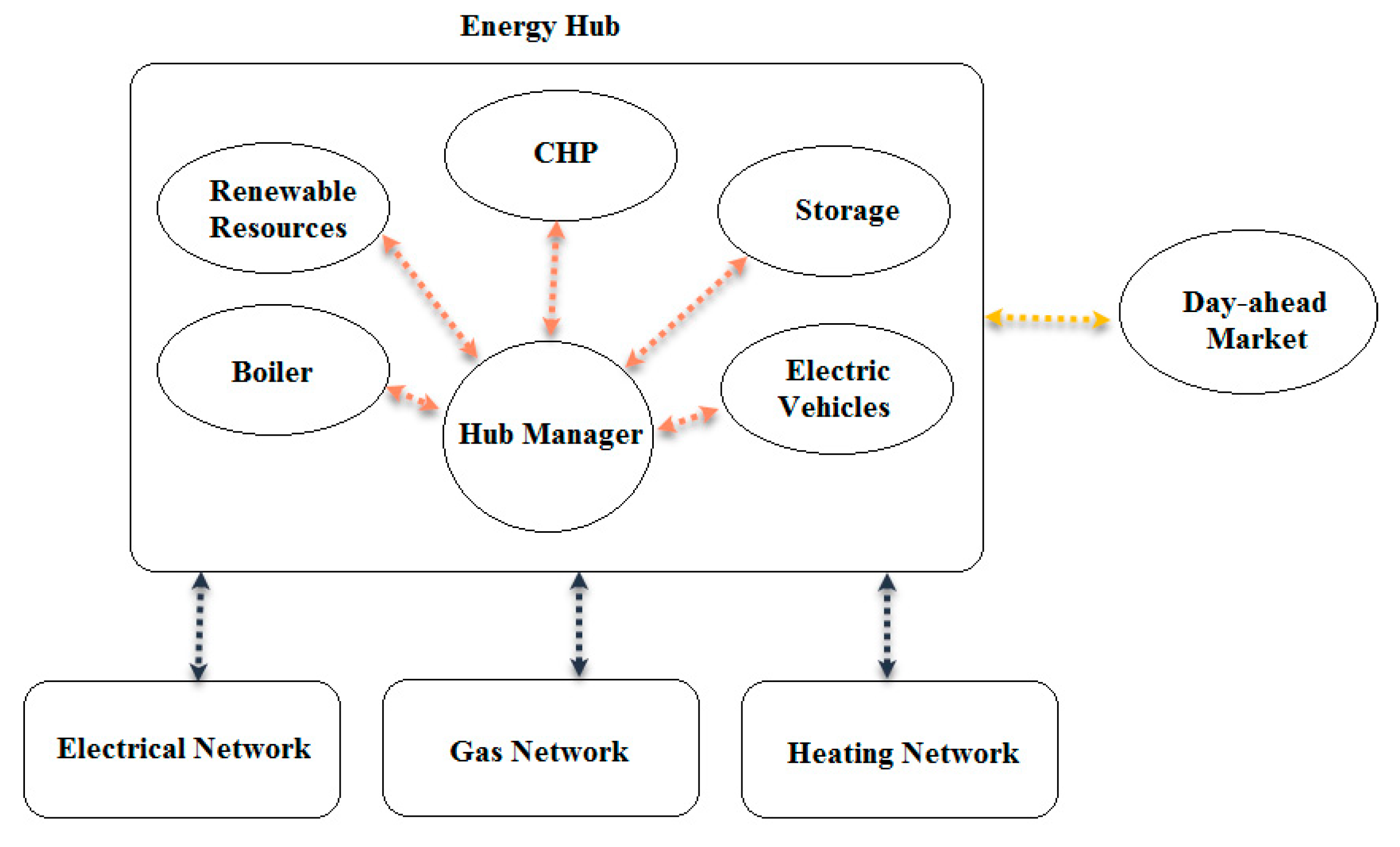
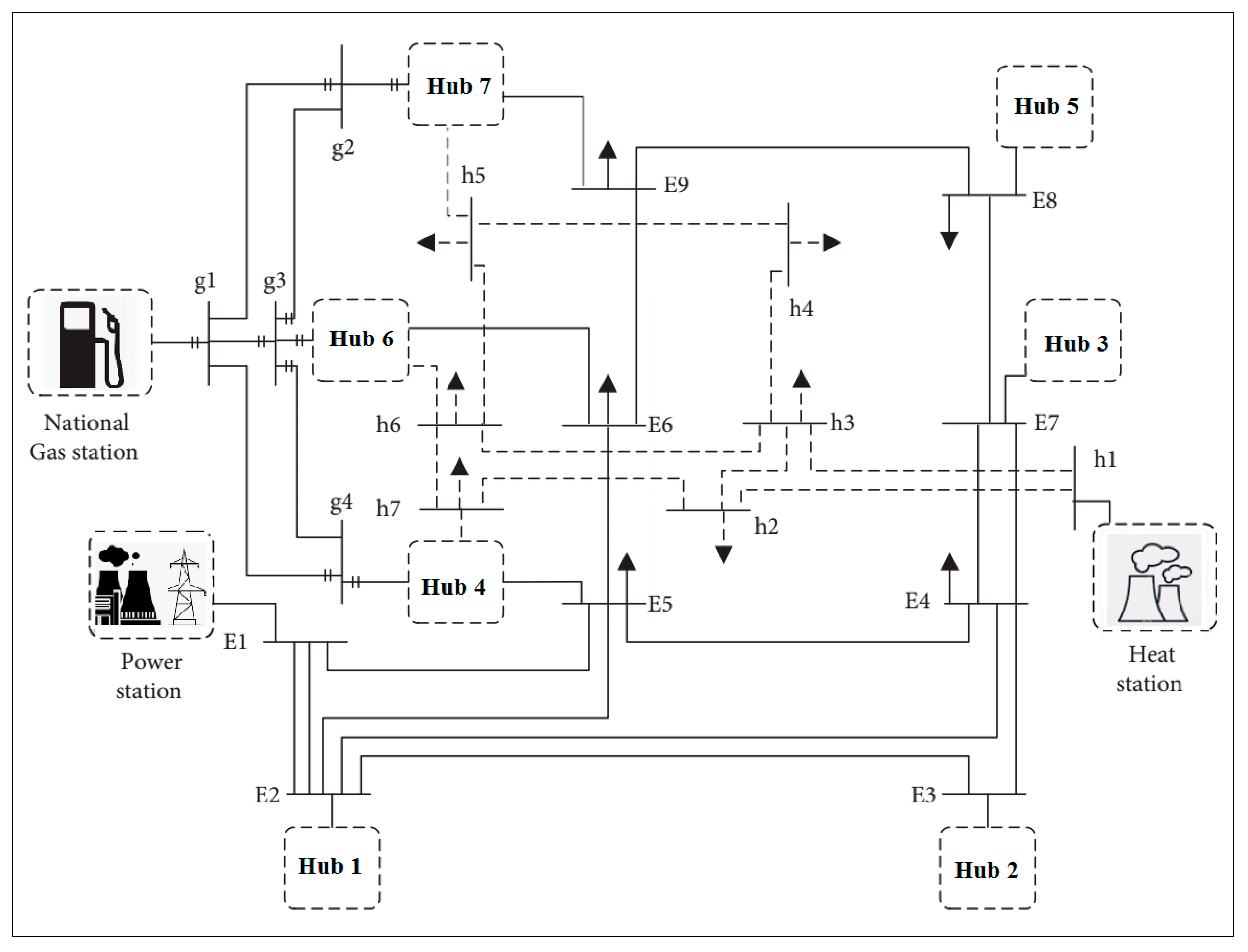
In this section, the optimal EH scheduling is presented with participation in EGHNs, taking into account the day-ahead market with the objective function of maximizing energy profit and with the constraints of network operation and hubs. In the following, the EH model and objective framework are described.

2.1. EH System

The optimal EH scheduling framework is presented in Figure 1 for EH scheduling in the electricity, gas, and heating day-ahead market. The provided EH includes photovoltaic energy sources, wind energy sources, CHP, boilers, storage elements, and electric parking lots based on electric vehicles (EVs), which work together to maximize the profit of the EH in the electricity, gas, and district heating day-ahead market. In this model, different electricity and natural gas, and district heating networks are considered. The purpose of the presented model is the optimal planning and simultaneous management of different energy hub equipment to achieve the best economic performance in the day-ahead market, and the system profit is affected by the price of electricity, natural gas, and heating energy. Therefore, all the equipment participates together under the hub energy planning and management in different networks to achieve maximum profit.

2.2. Objective Function

In this study, EH scheduling is presented in the market-facing EGHNs for profit maximization. The objective function of profit maximization of the EH includes the sale of active and reactive power in the electricity market, as well as the income of the EH in the day-ahead markets of natural gas and district heating, which is defined as follows:

$$Max Profit={\displaystyle \sum _{t={\mathrm{\Omega }}_t}{\displaystyle \sum _{m\in {\mathrm{\Omega }}_{Hub}}\left\{\left.{\lambda }_t^e(H_{m,t}^p+k_q\left|H_{m,t}^q\right|)+{\lambda }_t^g{H}_{m,t}^g+{\lambda }_t^h{H}_{m,t}^h\right\}\right.}}$$

(1)

2.3. Constraints of the Problem

In solving the optimization problem of hub energy scheduling, the objective function of the problem should be optimized under constraints. In other words, the problem is presented as a constrained optimization, taking into account various constraints, including network operation constraints and hub energy. In other words, the constraints of the problem must be satisfied in the process of solving the optimization problem in order to achieve a feasible solution. Here, the minimum and maximum capacity of each of the energy hub equipment is presented to the program, in which case the optimization program is allowed to explore to determine the optimal capacity of each equipment in the defined search space. On the other hand, other constraints include the current and voltage constraints of the power grid, which must be within the minimum and maximum allowed limits in the process of solving the optimization problem. In the optimization program, for linking constraints to the program, a penalty value is defined as a very large number for each constraint. To escape from that penalty value, the optimization program tries to maintain the capacity of the equipment and the network flow at its allowed value. In this way, the problem of scheduling is bound.

In the following, the network operation and EH constraints are presented.

2.3.1. Power Flow Constraint

The power flow constraints in EGHNs are presented below [25,26,27].

• The active and reactive power balance in different buses

$$D{S}_{e,t}^p-S_{e,t}^p+{\displaystyle \sum _{m{\in }_{Hub}}A{H}_{e,m}^e{H}_{m,t}^p}={\displaystyle \sum _{j\in {\mathrm{\Omega }}_e}{A}_{e,j}^e{F}_{e,j,t}^p} \forall e,t$$

(2)

$$D{S}_{e,t}^q-S_{e,t}^q+{\displaystyle \sum _{m{\in }_{Hub}}A{H}_{e,m}^e{H}_{m,t}^q}={\displaystyle \sum _{j\in {\mathrm{\Omega }}_e}{A}_{e,j}^e{F}_{e,j,t}^q} \forall e,t$$

(3)

• Active and reactive power flow of lines

$$F_{e,j,t}^p=G_{e,j}{(V_{e,t})}^2-V_{e,t}{V}_{j,t}\left\{\left.G_{e,j}\cos ({\delta }_{e,t}-{\delta }_{j,t})+B_{e,j}\sin ({\delta }_{e,t}-{\delta }_{j,t})\right\}\right. \forall e,t$$

(4)

$$F_{e,j,t}^q=-B_{e,j}{(V_{e,t})}^2+V_{e,t}{V}_{j,t}\left\{\left.B_{e,j}\cos ({\delta }_{e,t}-{\delta }_{j,t})-G_{e,j}\sin ({\delta }_{e,t}-{\delta }_{j,t})\right\}\right. \forall e,t$$

(5)

• Voltage angle in the base bus

The voltage angle in the base bus should follow the ${\delta }_{e,t}=0_{ \forall e=Slack bus,t}$.

• Balance of gas power and flow

The balance of gas power in different buses and gas flow through the pipeline at hour t is as follows:

$$G{S}_{g,t}-L_{g,t}^g+{\displaystyle \sum _{m{\in }_{Hub}}A{H}_{g,m}^g{H}_{m,t}^g}={\displaystyle \sum _{j\in {\mathrm{\Omega }}_g}{A}_{g,j}^g{F}_{g,j,t}^g \forall g,t}$$

(6)

$$F_{g,j,t}^g={\kappa }_{g,j}\mathrm{si}gn({\pi }_{g,t},{\pi }_{j,t})\sqrt{sign({\pi }_{g,t},{\pi }_{j,t})({\pi }_{g,t}^2,{\pi }_{j,t}^2)} \forall g,j,t$$

(7)

• The heating power balance in buses

$$H{S}_{h,t}-L_{h,t}^h+{\displaystyle \sum _{m{\in }_{Hub}}A{H}_{h,m}^h{H}_{m,t}^h}={\displaystyle \sum _{j\in {\mathrm{\Omega }}_g}{A}_{h,j}^h{F}_{h,j,t}^h} \forall h,t$$

(8)

• Heat power flow

Heat power flow through a pipeline at time t is as follows:

$$F_{h,j,t}^h=c_{h,j}{\dot{m}}_{h,j}(T_{h,t}-T_{j,t}) \forall h,j,t$$

(9)

2.3.2. Network Operation Constraints

In this section, operation constraints in EGHNs are presented. These constraints are defined in Equations (10)–(18).

• Voltage range of buses

$$V_e^{\min }\le V_{e,t}\le V_e^{\max } \forall e,t$$

(10)

• Allowed capacity of lines and stations

$$\sqrt{{(F_{e,j,t}^p)}^2+{(F_{e,j,t}^q)}^2}\le F_{e,j}^{e,\max } \forall e,j,t$$

(11)

$$\sqrt{{(D{S}_{e,t}^p)}^2+{(D{S}_{e,t}^q)}^2}\le D{S}_e^{\max } \forall e,t$$

(12)

• Bus pressure limit

$${\pi }_g^{\min }\le {\pi }_{g,t}\le {\pi }_g^{\max } \forall g,t$$

(13)

• The capacity of gas pipes and station

$$-F_{g,j}^{g,\max }\le F_{g,j,t}^g\le F_{g,j}^{g,\max } \forall g,j,t$$

(14)

$$-G{S}_g^{\max }\le G{S}_{g,t}\le G{S}_g^{\max } \forall g,t$$

(15)

• The thermal limit of buses

$$T_h^{\min }\le T_{h,t}\le T_h^{\max } \forall h,t$$

(16)

• The capacity of the station and heating pipeline

$$-F_{h,j}^{h,\max }\le F_{h,j,t}^h\le F_{h,j}^{h,\max } \forall h,j,t$$

(17)

$$-H{S}_h^{\max }\le H{S}_{h,t}\le H{S}_h^{\max } \forall h,t$$

(18)

2.3.3. EH Constraints

In this study, the presented EH includes photovoltaic and wind renewable energy sources, storage, electric parking, CHP, and boilers, and is connected to the electricity, gas, and regional heating network for the ability to deliver/receive energies. The active powers of gas output and heating of the hub are calculated based on Equations (19)–(22).

$$H_{m,t}^p=CH{P}_{m,t}^p+RE{S}_{m,t}+(S{T}_{m,t}^{p,dch}-S{T}_{m,t}^{p,ch})+(E{V}_{m,t}^{p,dch}-E{V}_{m,t}^{p,ch})-H{D}_{m,t}^p \forall m,t$$

(19)

$$H_{m,t}^q=CH{P}_{m,t}^q+S{T}_{m,t}^q+E{V}_{m,t}^q-H{D}_{m,t}^q \forall m,t$$

(20)

$$H_{m,t}^g=-CH{P}_{m,t}^g+B{O}_{m,t}^g-H{D}_{m,t}^g \forall m,t$$

(21)

$$H_{m,t}^h=CH{P}_{m,t}^h+B{O}_{m,t}^h-H{D}_{m,t}^h \forall m,t$$

(22)

The power balance equation of the CHP is presented in Equation (23) concerning the CHP power boundaries in the gas network (Equation (24)), in the electricity network (Equation (25)), and the heating network (Equation (26)).

$$CH{P}_{m,t}^g=\frac{(CH{P}_{m,t}^g+CH{P}_{m,t}^h)}{{\eta }^{CHP}} \forall m,t$$

(23)

$$0\le CH{P}_{m,t}^h\le CH{P}_m^{h,\max } \forall m,t$$

(24)

$$\sqrt{{(CH{P}_{m,t}^p)}^2+{(CH{P}_{m,t}^q)}^2}\le CH{P}_m^{e,\max } \forall m,t$$

(25)

$$0\le CH{P}_{m,t}^h\le CH{P}_{m,t}^{h,\max } \forall m,t$$

(26)

The constraints related to the storage system are presented based on Equations (27)–(32). These constraints are based on the stored energy (Equation (25)), charge and discharge range (Equations (28) and (29)), primary energy range (Equation (30)), stored energy range (Equation (31)), as the limit of the charger (Equation (32)).

$$E_{m,t+1}^{ST}=E_{m,t}^{ST}+{\eta }^{ST,ch}S{T}_{m,t}^{p,ch}-\frac{1}{{\eta }^{ST,dch}}S{T}_{m,t}^{p,dch} \forall m,t$$

(27)

$$0\le S{T}_{m,t}^{p,ch}\le C{R}_m^{ST}s{t}_{m,t} \forall e,t$$

(28)

$$0\le S{T}_{m,t}^{p,dch}\le D{R}_m^{ST}(1-s{t}_{m,t}) \forall m,t$$

(29)

$$E_{m,t}^{ST}=E_m^{ini} \forall m,t=1$$

(30)

$$E_m^{\min }\le E_{m,t}^{ST}\le E_m^{\max } \forall m,t$$

(31)

$$\sqrt{{(S{T}_{m,t}^{p,dch}-S{T}_{m,t}^{p,ch})}^2+{(S{T}_{m,t}^q)}^2}\le S{T}_m^{\max } \forall m,t$$

(32)

The constraints related to the parking of EVs are presented as Equations (33)–(38) [25,26,27,28]. The energy stored in the battery of EVs is calculated using Equation (33). The charging and discharging capacity of EVs are defined in Equations (34) and (35). The specification of the battery banks when EVs enter and exit the parking lot can be provided by Equations (36) and (37) and the specification of the EV charger capacity is presented in (38).

$$E_{m,t+1}^{EV}=E_{m,t}^{EV}+{\eta }^{EV,ch}{E}_{m,t}^{p,ch}-\frac{E_{m,t}^{p,dch}}{{\eta }^{EV,dch}} \forall m,t$$

(33)

$$0\le E_{m,t}^{EV,p,ch}\le C{R}_{m,t}^{EV}e{v}_{m,t} \forall m,t$$

(34)

$$0\le E_{m,t}^{EV,p,dch}\le D{R}_{m,t}^{EV}(1-e{v}_{m,t}) \forall m,t$$

(35)

$$E_{m,t}^{EV}=E_{m,t}^{arr} \forall m,t=Arrival time$$

(36)

$$E_{m,t}^{EV}=E_{m,t}^{dep} \forall m,t=Departure time$$

(37)

$$\sqrt{{(E{V}_{m,t}^{p,dch}-E{V}_{m,t}^{p,ch})}^2+{(E{V}_{m,t}^q)}^2}\le E{V}_{m,t}^{\max } \forall m,t$$

(38)

In addition, the power balance equation of the boiler and size limits can be defined based on Equations (39)–(40) [18].

$$B{O}_{m,t}^g=\frac{B{O}_{m,t}^h}{{\eta }^{BO}} \forall m,t$$

(39)

$$0\le B{O}_{m,t}^g\le B{O}_m^{\max } \forall m,t$$

(40)

$E{V}^{\max }$ is equivalent to ${{\displaystyle \sum }}_{i=1}^{N_{1t}}C{C}_i^{ev}$, which indicates $C{C}^{ev}$ is the charging capacity of the EVs. $E^{arr}/E^{dep}$ is equivalent to ${{\displaystyle \sum }}_{i=1}^{N_{2t}}SO{C}_{i}B{C}_i/{{\displaystyle \sum }}_{i=1}^{N_{3t}}B{C}_i$, in which SOC expresses the state of charge and $BC$ is the battery capacity of any EVs. $N_{2t}$ and $N_{3t}$ also refer to the arrival and departure times of EVs.

3. Proposed Optimization Method

3.1. Overview of the FLA

The Fick diffusion law has been adopted in structuring a new optimization tool and is employed in the present research for optimal scheduling of the EH. The FLA includes diffusion, equilibrium, and steady-state phases. The FLA is a powerful optimization method that can fairly perform exploration and exploitation processes by balancing these phases [31].

3.1.1. Inspiration

The motion of particles between different concentrated points in the space follows the Fick diffusion equations. It states that “diffusion speed is directly related to surface area and concentration difference and has a reverse relationship with the membrane thickness”. Diffusion based on the rules of Fick is called normal propagation or Fick. In the FLA algorithm, Fick’s law is simulated so that stable positions of molecules are found. In this algorithm, three motion operators including (1) a diffusion operator (DO), (2) an equilibrium operator (EO), and (3) a steady-state operator (SSO) are provided. In the DO phase, it is assumed that there are two regions at the beginning of the experiment with considerable concentration differences, which forces the particles to move and replace other particles’ positions. In the EO phase, the two concentrations are approximately the same and the particles attempt to find an equilibrium. The SSO phase happens when particles change their positions region based on the most desirable location.

3.1.2. Formulation of FLA

The FLA algorithm is mathematically presented as described below.

• Step 1: Initialization. In the FLA, optimization starts based on several preferred solutions, shown by X, according to Equation (41). The generation of solutions is random and in each iteration, the best solution is selected as the best current almost optimal solution [29].

  $$\mathrm{X}=\left[\begin{array}{cccc}{x}_{1,1}& x_{1,\mathrm{j}}& \cdots & \cdots \\ x_{2,1}& x_{2,\mathrm{j}}& \cdots & \cdots \\ ⋮& ⋮& ⋮& ⋮\\ \begin{array}{c}⋮\\ x_{\mathrm{N},1}\end{array}& \begin{array}{c}⋮\\ x_{\mathrm{N},\mathrm{j}}\end{array}& \begin{array}{c}⋮\\ \cdots \end{array}& \begin{array}{c}⋮\\ x_{\mathrm{N},\mathrm{D}}{}_{-1}\end{array}\end{array}\begin{array}{c}{x}_{1,\mathrm{D}}\\ x_{1,\mathrm{D}}\\ ⋮\\ \begin{array}{c}⋮\\ x_{\mathrm{N},\mathrm{D}}\end{array}\end{array}\right]$$

  (41)

  where N represents the number of solutions (population size), D represents the dimension of the problem (number of variables), and j refers to the jth decision variable.
• Step 2: Clustering. In this step, the population of the algorithm is divided into two equal groups, N1 and N2.
• Step 3: Transfer function (TF). The efficiency of any algorithm is highly dependent on the transition from discovery to exploitation, and vice versa. In the FLA, a nonlinear transfer function (TF) is provided for this problem. TF function is defined as Equation (42) [29].

  $$T{F}^t=\sinh {(t/T)}^{c1}$$

  (42)

Here, t and T show the number of iterations and the maximum number of iterations, and C1 is considered 0.5.

• Step 4: Update the molecule position: In this step, three phases based on transfer operators, namely DO, EO, and SSO, are presented. The transition process between the three phases is based on the following equation [31]:

  $$X_i^t=\left\{\begin{array}{l}DO T{F}^t<0.9\\ EO T{F}^t\le 1\\ SSO T{F}^t>1\end{array}\right.$$

  (43)

3.1.3. DO Operator (Discovery Phase)

If there is a high concentration difference between two regions, molecules change their position according to the region concentration. $T_{DO}^t$ is defined as follows [29].

$$T_{DO}^t=C_5\times T{F}^t-r, C_5=2$$

(44)

The flow direction is determined according to the value of $T_{DO}^t$ as follows [29]:

$$X_{p,i}^t=\left\{\begin{array}{l}from i to j region T_{D0}^t< rand\\ from j to i region otherwise\end{array}\right.$$

(45)

If the concentration of region i is higher than that of region j, some molecules will migrate from region i to region j, and other remaining molecules in region i are influenced by this movement. The number of molecules transferred ($N{T}_{ij}$) and the number of remaining molecules within molecular group i ($N{R}_{ij}$) can be defined as follows [31]:

$$N{T}_{ij}\approx N_i\times r_1\times (C_4-C_3)+N_i\times C_3, N{R}_{ij}\approx N_i-N{T}_{ij}$$

(46)

NT_ij means transferred molecules then move to another region and their position is mainly updated concerning the most favorable equilibrium molecule in area j as follows [29]:

$$X_{p,i}^{t+1}=X_{EO,j}^t+D{F}_{p,j}^t\times DOF\times r_2\times (J_{i,j}^t\times X_{EO,j}^t-X_{p,j}^{t+1})$$

(47)

Furthermore, DOF indicates the time-varying flow direction, which is defined as Equation (48) [29].

$$DOF=\exp (-C_2(T{F}^t-r_1)), C_2=2$$

(48)

J^t_i,j refers to the diffusion flux considering effective diffusion constant (D) and concentration gradient (concentration gradient), which is presented as follows [29]:

$$J_{i,j}^t=-D\frac{d{c}_{i,j}^t}{d{x}_{i,j}^t}$$

(49)

$d{c}_{i,j}^t$ and $d{x}_{i,j}^t$ are obtained considering the average position of the molecule in regions i and j (X^t_m,j and X^t_m,i) as follows [29]:

$$d{c}_{i,j}^t=X_{m,j}^t-X_{m,i}^t$$

(50)

$$d{x}_{i,j}^t=\sqrt{{(x_{EO,j}^t)}^2-{(x_{p,i}^t)}^2+eps}$$

(51)

The position of remaining molecules in the ith group in region i is updated based on the movement between distinct stages (equilibrium positions in regions i and j and problem boundary and no change in the positions). This strategy can be described by Equation (52) [29] considering the equilibrium point in area i (X^t_EO,i) and upper (U) and lower (L) limits of the problem:

$$X_{p,j}^{t+1}=\left\{\begin{array}{l}{X}_{EO,i}^t rand<0.8\\ X_{EO,i}^t+DOF\times (r_3\times (U-L)+L rand<0.9\\ X_{p,i}^{t+1} otherwise\end{array}\right.$$

(52)

Molecules in region j modify their position in the same region due to their higher concentration without traveling; that is, their position is updated relative to the equilibrium point. The problem boundary is defined by Equation (53) [29]:

$$X_{p,j}^{t+1}=X_{EO,j}^t+DOF\times (r_4\times (U-L)+L$$

(53)

3.1.4. EO Operator (Transition Stage from Exploration to Exploitation)

In this step, the exploration phase is transferred to exploitation. The position of molecules is updated considering the location of particle p in the group (X^t_p,g) and the equilibrium position in group g (X^t_EO,g), based on Equation (54) [29].

$$X_{p,g}^{t+1}=X_{EO,p}^t+Q_{EO,g}^t\times X_{p,g}^t+Q_{EO,g}^t\times (M{S}_{p,EO}^t\times X_{EO,g}^t-X_{p,g}^t)$$

(54)

The relative quantity of the region in group g (Q^t_EO,g) and the diffusion rate coefficient in group (DRF^t_EO,g), as in Equations (55) and (60) [29], are defined as follows:

$$Q_{EO,g}^t=R_1^t\times D{F}_g^t\times DR{F}_{EO,g}^t$$

(55)

$$DR{F}_{EO,g}^t=\exp (-\frac{J_{p,EO}^t}{T{F}^t})$$

(56)

$$J_{p,EO}^t=-D\frac{d{c}_{g,EO}^t}{d{x}_{p,EO}^t}$$

(57)

dc^t_g,EO and dx^t_p,EO are determined as follows [29]:

$$d{c}_{g,EO}^t=x_{g,EO}^t-X_{m,g}^t$$

(58)

$$d{x}_{p,EO}^t=\sqrt{{(x_{g,EO}^t)}^2-{(x_{p,g}^t)}^2+eps}$$

(59)

$$D{F}_g^t=\pm 1 direction factor$$

(60)

$$M{S}_{p,EO}^t=\exp (-\frac{F{S}_{g,EO}^t}{F{S}_{p,g}^t+eps}) motion step$$

(61)

$$R_1^t=rand{[0,1]}_d d=1 : \dim ension$$

(62)

3.1.5. Steady State Operator (SSO) (Exploitation Phase)

The exploitation phase is the final step in the optimization problem. In this step, the position of the molecules will be updated considering the location of the steady state (X^t_SS) and the position of the p particle (X^t_p,g) based on the following equation [29]:

$$X_{p,g}^{t+1}=X_{ss}^t+Q_g^t\times X_{p,g}^t+Q_g^t\times (M{S}_{p,g}^t\times X_{ss}^t-X_{p,g}^t)$$

(63)

Q^t_g and MS^t_p,EO express the relative quantity of area g and refer to the transition phase, which is determined by [29]

$$Q_g^t=R_1^t\times D{F}_g^t\times DR{F}_g^t$$

(64)

In Equation (64), DF^t_p represents the direction factor equal to ±1, R^t₁ randomly varies between [0, 1] and DRF^t_p expresses the signal diffusion speed factor, which is obtained as follows [29]:

$$DR{F}_g^t=\exp (-\frac{J_{p,ss}^t}{T{F}^t})$$

(65)

$$M{S}_{p,g}^t=\exp (-\frac{F{S}_{ss}^t}{F{S}_{p,g}^t+eps})$$

(66)

J^t_p,ss is determined as follows [29]:

$$J_{p,ss}^t=-\frac{d{c}_{g,ss}^t}{d{x}_{p,ss}^t}$$

(67)

dc^t_g,ss and dx^t_p,ss are calculated based on the following equations [29]:

$$\begin{array}{l}d{c}_{g,ss}^t=x_{m,g}^t-X_{ss}^t\\ d{x}_{p,ss}^t=\sqrt{{(x_{ss}^t)}^2-{(x_{p,g}^t)}^2+eps}\end{array}$$

(68)

3.1.6. Balancing the Exploration and Exploitation Phases

Establishing a balance between the exploration and exploitation phases is essential when dealing with optimization algorithms. The FLA consists of diffusion, equilibrium, and steady-state steps. Exploration is based on a simulated diffusion phase, by which molecules discover the entire search domain. Then, the transition between exploration and exploitation can be implemented based on the equilibrium stage. Finally, following the steady state stage, the exploitation of molecules from promising areas is established.

3.1.7. FLA Pseudo Code

Algorithm 1 shows the step-by-step process of the FLA.

Algorithm 1. Steps of implementation of the FLA

1: Initialization;

2: Insert parameters  of D, C1, C2, C3, C4, C5;

3: Initiate the population Xi (i = 1, 2, … N) as random;

4: Clustering: Dividing the population into two groups N1, and N2;

5: for s = 1:2 do

6: Calculate the fitness of each group molecule Ns;

7: Determining the best molecule is the best fitness value;

8: end for

9: while FES ≤ MAXFES do

10: if If TF is greater than 0.9 then: (SSO)

11: for op = 1: nop do

12: Compute the rate of diffusion via Equation (65)

13: Compute the step of motion factor via Equation (66)

14: Update the position of the population via Equation (63)

15: end for

16: else if TF is fewer than rand then (EO)

17: for op = 1: nop do

18: Compute rate of diffusion via Equation (56)

19: Compute quantity of group relative via Equation (55)

20: Update position of the population via Equation (54)

21: end for

22: else (EO)

23: Compute flow direction via Equation (48)

24: calculate molecules number tending to move to region via Equation (46)

25: Update position of the population via Equation (47)

26: Update remained molecules in the region i via Equation (52)

27: Update the region j molecules via Equation (53)

28: Update FES ← FES + NP

29: end while

30: Return best solution.

3.2. Overview of the IFLA

The traditional FLA algorithm has problems in the form of an imbalance between exploration and exploitation, as well as getting caught in premature convergence. In this study, to improve the performance of the traditional FLA algorithm against these problems, Rosenbrock’s direct rotational (RDR) method [30] is used. In this method, the coordinate axes are the initial search path in the RDR local search method, which rotates along these directions before moving to a new set point where effective steps are generated until at least one effective process and one unsuccessful step in any search direction.

In this case, the current phase is finished and the identification basis is checked to calculate the cumulative effect of all successful phases in all dimensions [30]. The orthonormal basis is updated as follows [30]:

$$x^{k+1}-x^{k+}={\displaystyle \sum _{i=1}^n{\lambda }_i.d_i}$$

(69)

In the equation below, a set of instructions is provided. Where λ_i represents the total number of successful variables, and $x^{k+1}-x^{k+}$ represents the point with the most useful search direction. Therefore, it is placed in the corrected search direction [30].

$$pi=\left\{\begin{array}{l}{d}_i, {\lambda }_i=0\\ {\displaystyle \sum _{j=0}^n{\lambda }_j.d_j {\lambda }_i\ne 0}\end{array}\right.$$

(70)

Next, the search results based on the Gram-Schmidt normalization process are updated as the following equation [30].

$$qi=\left\{\begin{array}{l}{p}_i, i=1\\ p_i-{\displaystyle \sum _{j=1}^{i-1}\frac{q_j^T.p_i}{q_j^T.q_j} i\ge 2}\end{array}\right.$$

(71)

The modified and normalized search guidelines are defined as follows [30].

$$d_i=\frac{q_i}{‖q_i‖}, i=1,2,3,\dots ,n.$$

(72)

After updating the local search, this method performs the search operation until the convergence condition of the algorithm is met in the new opposite direction.

4. Simulation Results and Discussion

Here, the results obtained from EH scheduling and management in different networks in the day-ahead markets facing EGHNs are presented. The EH scheduling problem is presented as an optimization problem with the aim of maximizing the profit of hubs. In this study, the IFLA algorithm has been employed to optimize the problem under study, and a comparison is made between the suggested algorithm and conventional FLA, PSO, and MRFO. Population size, maximum iteration, and independent executions of each algorithm are selected as 100, 200, and 25, respectively.

Table 1. Control parameters of different algorithms.

Algorithm	Parameter	Value
FLA [29]	C	0.1
PSO [32]	C1	2
	C2	2
	Inertia weight	Linearly reduction from 0.9 to 0.1
MRFO [33]	S	2

lists the control parameters of the algorithms. It should be noted that the control parameters of different methods are the values provided by their authors in reference papers. In this study, the parameters of the conventional FLA algorithm are considered the same as the parameters set by its authors. Although the authors have checked the setting of these parameters and found that the parameters set by the authors of the algorithm provide the best results for base simulation with the FLA.

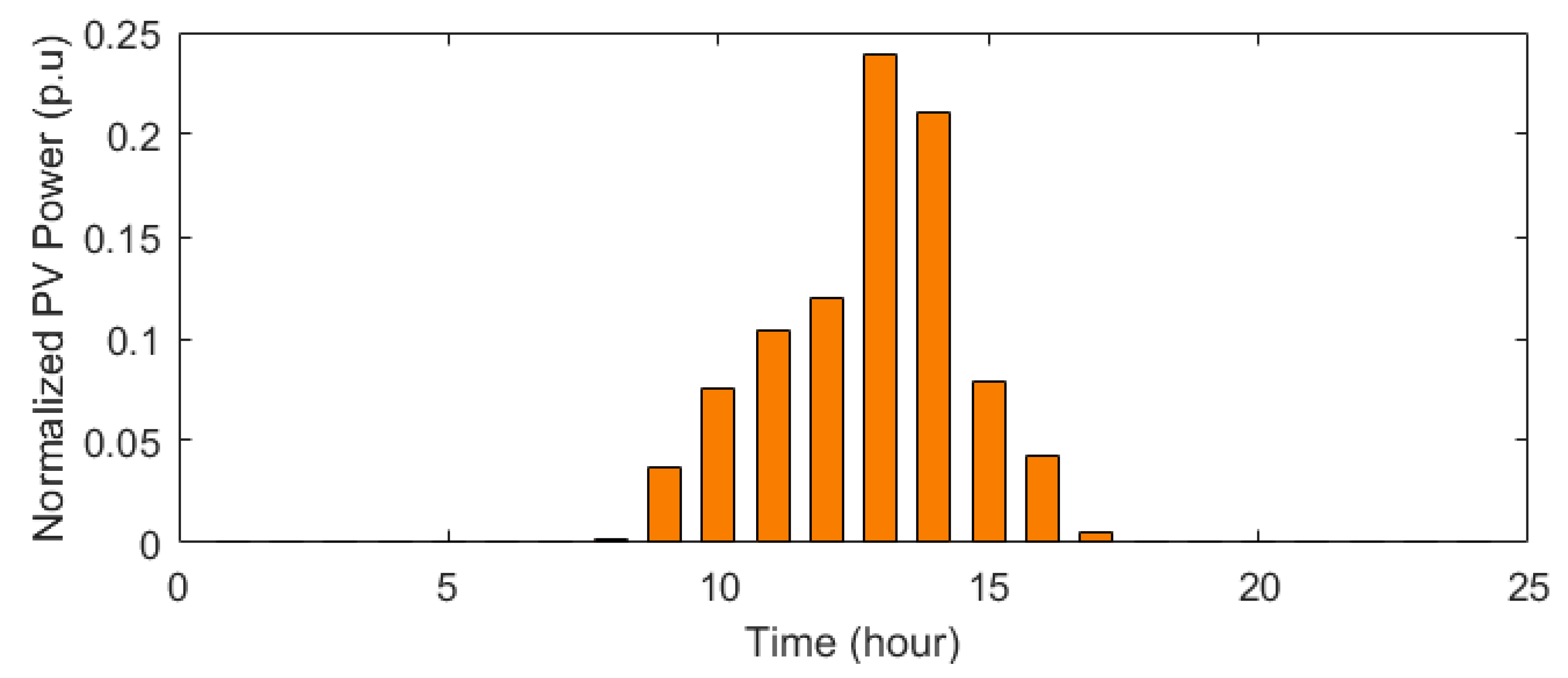
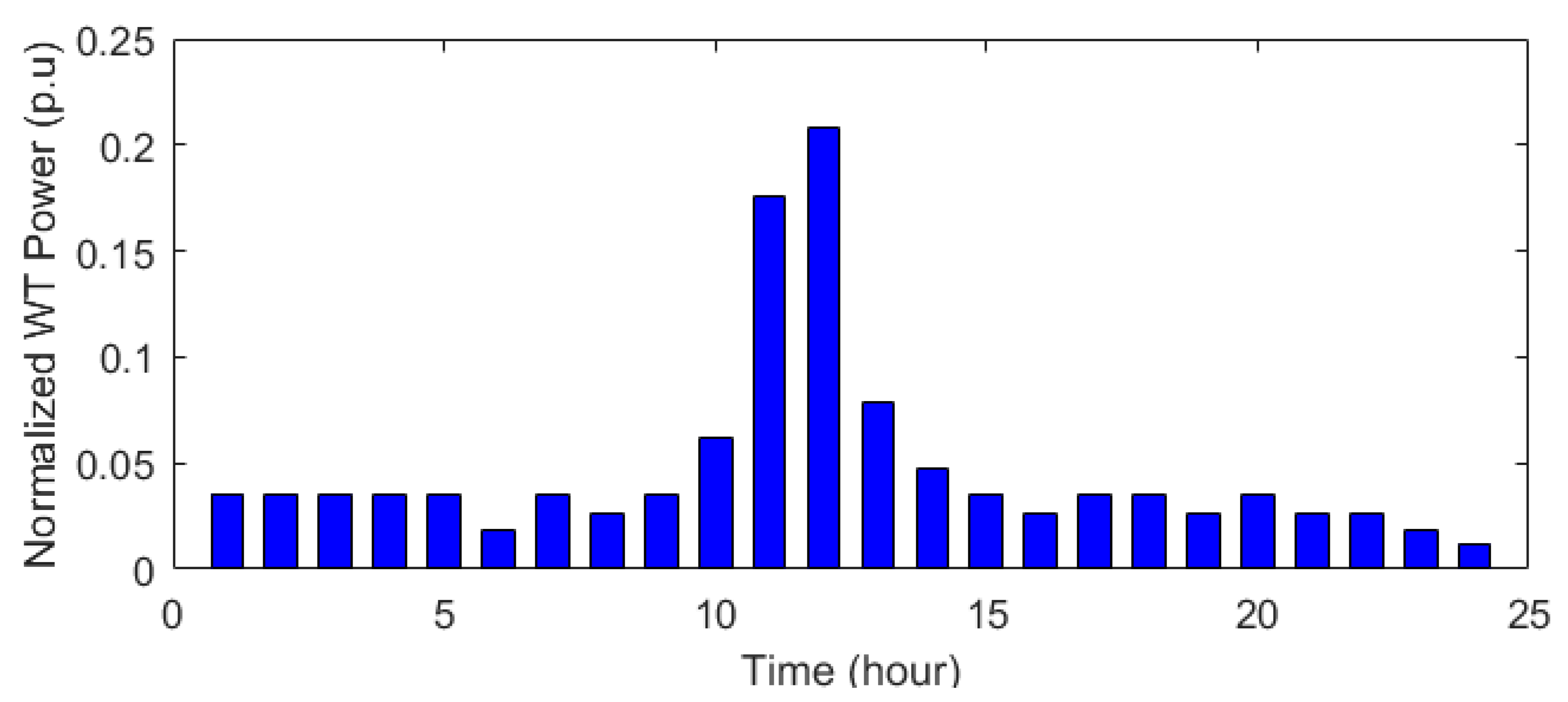
4.1. System under Study and Data

The studied system is a nine-bus electrical network, the number of lines of which is twelve, and it has four buses and five pipelines in the gas network and the urban heating network has nine buses and also has nine pipelines (Figure 2). Line/pipeline data, by assuming 1 MW as base power, a 1 kV base voltage, a 10-bar base pressure, and a 100 °C base temperature, are presented in

Table 2. Data of transmission lines, gas, and heating pipelines (p.u).

Electrical Network				Natural Gas Network				District Heating Network
Line	R	X	Fe,max	Pipeline	$\kappa$	sign	Fg,max	Pipeline	$c\times \dot{m}$	Fh,max
1-2	0.02	0.06	0.90	1-2	3	1	1.1	1-2	15	1.00
1-5	0.05	0.12	0.50	1-3	3.5	1	3.0	1-3	18.5	1.30
2-3	0.05	0.12	0.65	1-4	4	1	1.2	2-3	17.5	0.20
2-4	0.06	0.08	0.75	2-3	4.5	-1	0.6	2-7	18.5	0.50
2-5	0.06	0.11	0.80	3-4	4.5	1	0.8	3-4	19.5	0.65
3-4	0.07	0.11	1.20					3-6	19	0.20
4-5	0.01	0.04	0.65					4-5	15	0.35
4-7	0.01	0.03	0.90					5-6	19	0.10
5-6	0.02	0.05	1.10					6-7	19.5	0.20
6-9	0.10	0.09	0.30
7-8	0.02	0.07	1.30
8-9	0.08	0.12	0.35

[31]. Furthermore, the amplitude of voltage, pressure, and temperature can vary between 0.9 and 1.1 p.u. Moreover, the data of the system load in the electric load peak hour [31] is considered. These data include active and reactive load power (p.u) and heating load power (p.u). In the rest of the hours, the load percentage value is multiplied by the load value at 20:00.

The load curve (the share of peak load) of electric and heating networks is shown in Figure 3. Furthermore, Figure 4 illustrates the daily energy price curve in the day-ahead market for electricity, gas, and district heating energy. The size of electricity, gas, and heating stations is assumed to be 7, 11, and 3 p.u. The system under study consists of seven hubs, the location and characteristics of which can be found in Figure 2 and

Table 3. Hub specifications.

System		Location *		RES	Storage	EVs	CHP	Boiler			Load + (p.u)
	E	G	h						HD P	HD q	HD h	HD g
Hub 1	2	-	-	√	√	√			0.8	0.4	0	0
Hub 2	3	-	-	√	√	√			0.5	0.3	0	0
Hub 3	7	-	-	√	√	√			0.6	0.4	0	0
Hub 4	5	4	7				√	√	0.2	0.1	0.3	0
Hub 5	8	-	-	√	√	√			0.4	0.2	0	0
Hub 6	6	3	6	√	√	√	√	√	0.4	0.2	0.2	0
Hub 7	9	2	5	√	√	√	√	√	0.4	0.2	0.2	0

* E: Electrical, G: gas, h: district heating. ⁺ HD and HD are the active and reactive demand power in the hub (p.u), HD and HD are the gas and heating demand power in the hub (p.u).

, respectively.

Hubs’ renewable energy sources include photovoltaic and wind sources, the predicted power of which is presented in Figure 5 and Figure 6, respectively [31]. These figures show the forecasted changes in photovoltaic and wind power for the day-ahead. In addition, the number of EVs for hubs 1, 2, 3, 5, 6, and 7 is considered to be 60. The data of battery SOC, BC, charge/discharge rate and EV efficiency, and penetration rate are considered every hour [28,34]. For an electric storage system in which the charger size is 0.5 p.u, minimum and maximum sizes of 0.5 and 2 p.u, charge/discharge rate, and efficiency are considered to be 0.3 and 0.88, respectively. Furthermore, the size of the CHP in EGHNs is 2.5, 1, 1 with an overall efficiency of 80% [32]. The size and efficiency of the boiler system are 1 and 0.8 p.u.

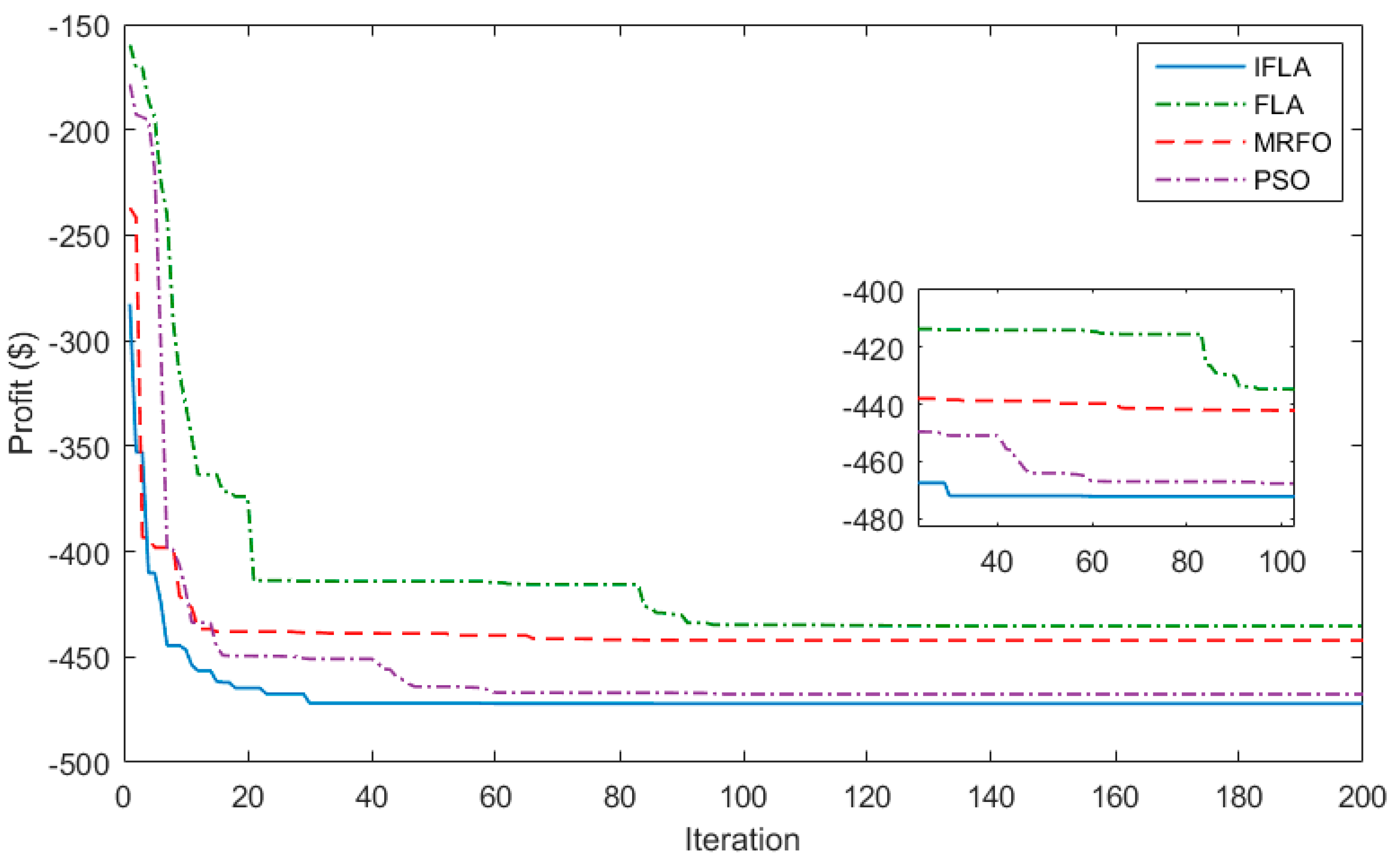
4.2. Superior Optimization Method

In this section, optimal energy scheduling and management of EH with the aim of maximizing profit are presented in the day-ahead markets in EGHNs by satisfying network operation constraints and hub constraints using IFLA’s new meta-heuristic algorithm. The performance of the proposed algorithm has been compared with conventional FLA, PSO, and MRFO. The convergence curve obtained from solving the problem by different algorithms is shown in Figure 7. Here, the value of the objective function represents the profit of the EH. According to the minimization in Matlab software and the objective of profit maximization, a negative sign is included in the objective function. As can be seen, the proposed method based on IFLA has obtained the optimal global solution with a higher profit value, higher convergence speed, and lower convergence tolerance in fewer convergence iterations compared to other methods. The numerical results of EH scheduling based on the proposed methodology are given in

Table 4. The numerical results obtained for various approaches to scheduling the EH.

Algorithm/Item	Convergence Iteration	Profit ($)	Algorithm Status	CPU Time (S)
IFLA	30	472.13	Globally optimal	155
FLA	91	435.34	Locally optimal	186
MRFO	66	442.17	Locally optimal	178
PSO	59	467.62	Locally optimal	167

. As is noted, the suggested approach based on IFLA achieved a profit of $472.13 in the 30th iteration, while other methods are stuck in the local optimum and are not able to achieve the global optimum. It can also be seen that the performance improvement of the conventional FLA method based on Rosenbrock’s direct rotational (RDR) method prevents the premature convergence of its improved version, while the traditional FLA method with a profit value of $435.34 has experienced premature convergence. Furthermore, in a statistical analysis of the performance of different algorithms according to

Table 5. The statistical analysis results of different methods in scheduling the EH.

Algorithm/Index	Best ($)	Worst ($)	Mean ($)	Std ($)
IFLA	472.13	461.78	469.24	46.37
FLA	435.34	419.65	428.03	94.46
MRFO	442.17	425.22	432.93	76.21
PSO	467.62	458.50	462.74	63.54

, the superior capability of the proposed algorithm has been confirmed in terms of achieving better statistical indices. The difference in the IFLA results compared to other methods is to achieve more profit of hub energy in the day-ahead electricity market. The proposed method has been able to get more profit from energy exchange with more accurate planning between energy resources and storage sources of the energy hub. The results showed that the proposed scheduling framework based on the IFLA based on a meta-heuristic algorithm has the ability to create a favorable balance between the phases of exploration and exploitation and is less able to determine the optimal solution in the convergence iteration. The results show that the use of a powerful optimization method can guarantee the optimal economic operation of the EH by satisfying the many constraints of the operation and the EH.

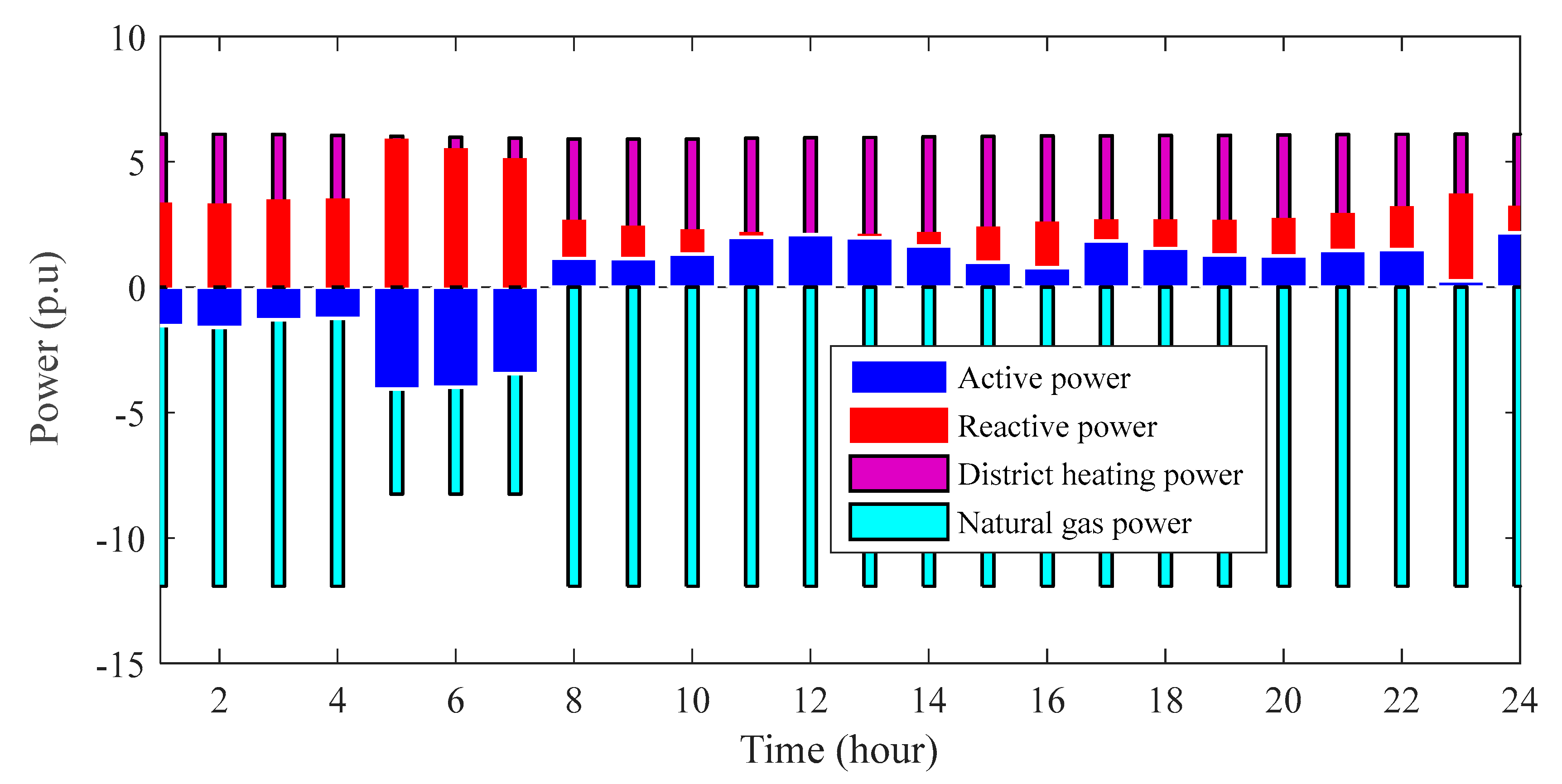
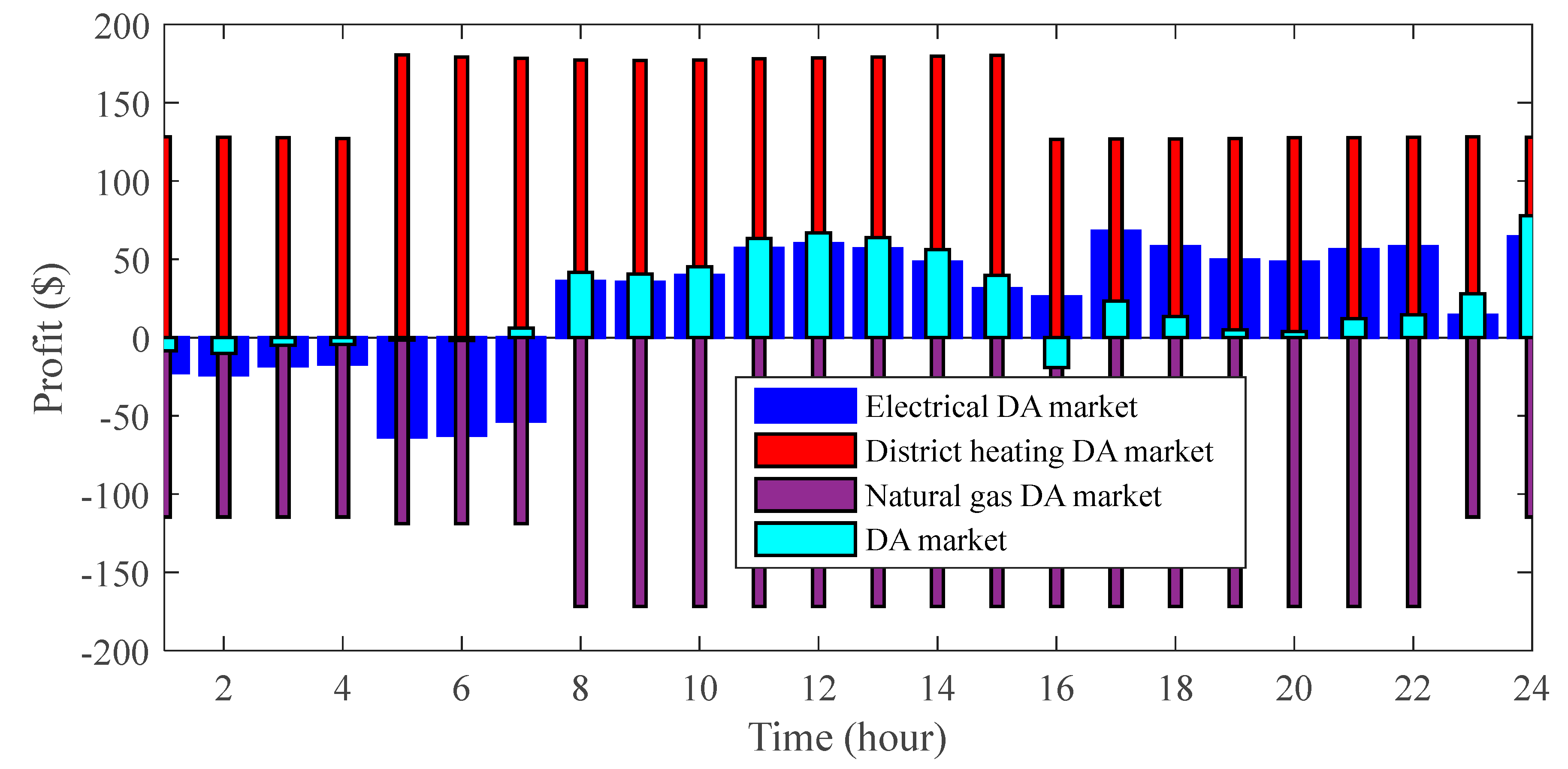
4.2.1. System Power and Profit

Figure 8 and Figure 9 show the power curve and daily profit for different energies, respectively. The optimal scheduling of the EH has been carried out by satisfying the operation and hub constraints using the IFLA algorithm. According to Figure 8, the active power of all EH equipment is not positive during the early hours of the program; i.e., 1:00 to 7:00. These conditions have been created because EVs are charging and energy is stored due to the low price of electricity in this period. On the other hand, the demand for hub equipment has been answered by CHP due to the low price of gas in the hours of 1:00 to 4:00. On the other hand, Figure 8 shows that due to the high price of electricity during the hours of 8:00 to 24:00, the electricity required by the networks is supplied by CHP equipment, renewable energy sources, storage systems, and electric vehicles during these hours. On the other hand, due to the higher price of heating energy compared to gas, the maximum allowed heating power has been delivered to the heating network during the full day. Therefore, from 1:00 to 4:00, power received in the hub equipment from the upstream network exceeds that of CHP, photovoltaic, and wind energy sources, and the power of the hub equipment is negative during these hours. Furthermore, in the hours of 8:00 to 24:00, the power of the hub equipment is positive. Therefore, according to the mentioned cases, energy management has been carried out to maximize the profit of the system.

The daily changes in the profit hub are presented in Figure 9. The results show that the profit of the system in the day-ahead market of different networks is affected by the price of energy. According to Figure 9, the benefit from heating is variable due to the variable price of heating energy in different periods. On the other hand, based on Figure 9, it is observed that the profit of the electricity market is negative in the hours 1:00 to 7:00 due to energy storage by the EVs, and it is positive in the rest of the hours. Furthermore, the profit earned in the gas market is not positive because of receiving gas energy from CHP and steam boilers, as well as the higher profit in the heating market compared to the gas market at all hours. The profit from the forward market includes the set of profits of all hubs in different forward markets in such a way that the negative profit means the positive cost.

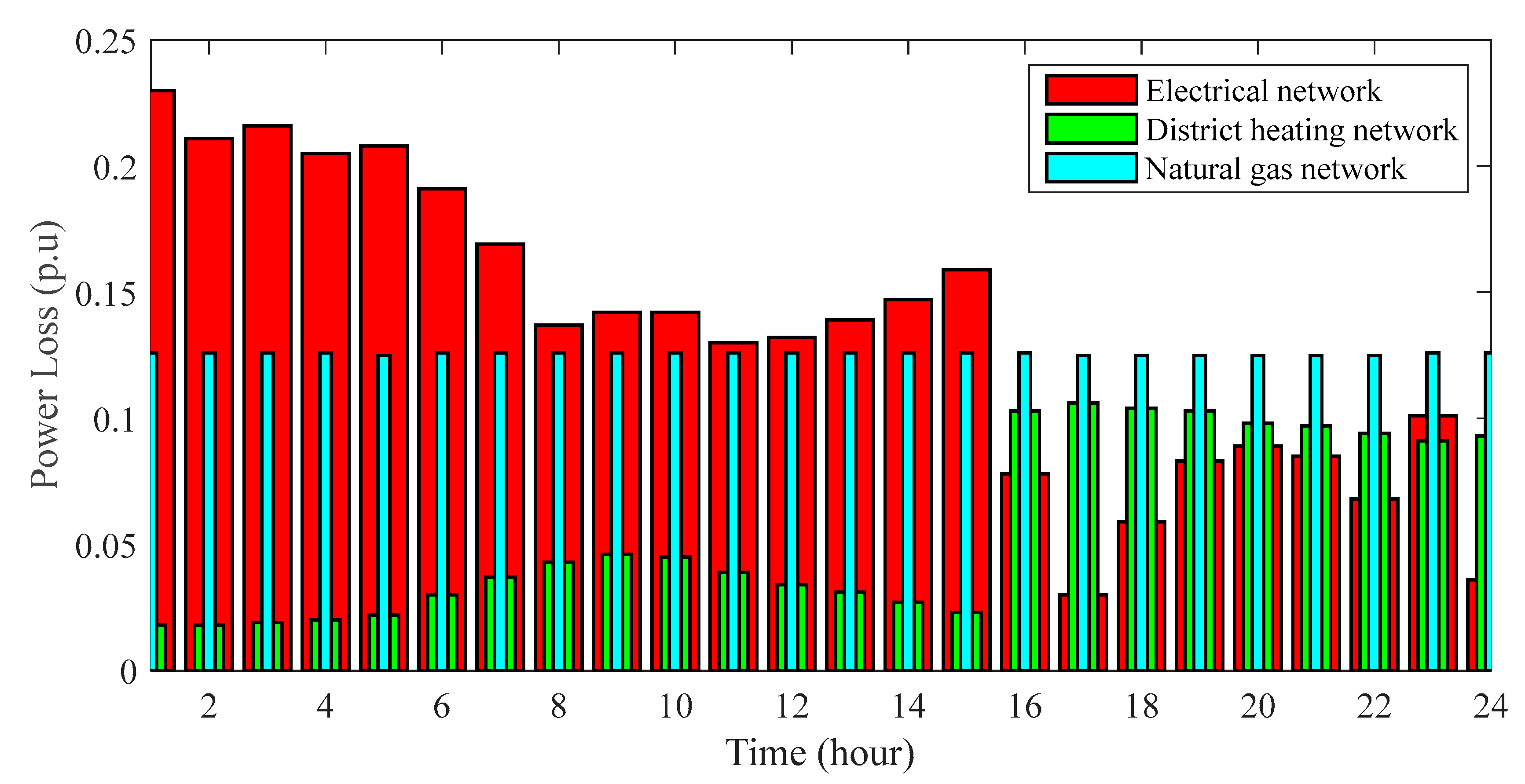
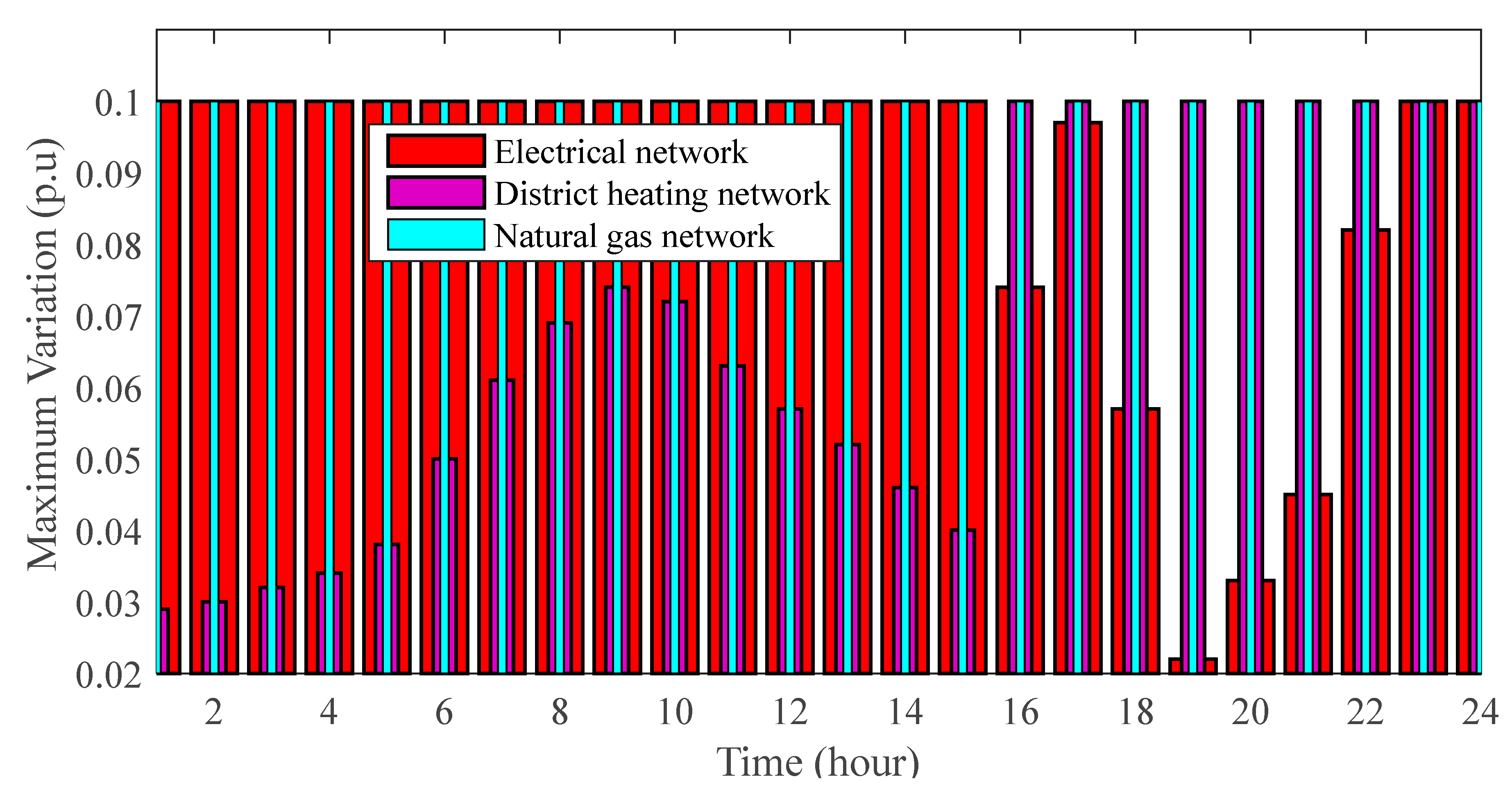
4.2.2. Network Loss and Deviations

Figure 10 shows the power loss changes in the electricity, heating, and gas markets. Due to the constant gas power in the hub and gas station, gas power losses are constant. According to Figure 10, the heating power loss from 1:00 to 15:00, which is low, has an increasing behavior over time, from 16:00 to 24:00. It can also be seen that the electric power loss is high between 1:00 and 7:00, which is due to the high demand of the EH during these hours.

In Figure 11, the daily changes in voltage deviation, pressure, and temperature in EGHNs are presented. For the gas network, the rate of change of 0.1 p.u for 24 h is reported because of the high gas demand in the EH. The temperature difference is also low for the hours from 1:00 to 15:00 and for the hours from 16:00 to 24:00, which is 0.1 p.u. In addition, the maximum voltage deviation occurred due to the demand of the EH and the power system in the time period 1:00 to 15:00 and 23:00 to 24:00, and the lowest voltage deviation occurred in the hours of 16:00 to 22:00, because of the delivery of active and reactive power above the hub into the power grid has been achieved.

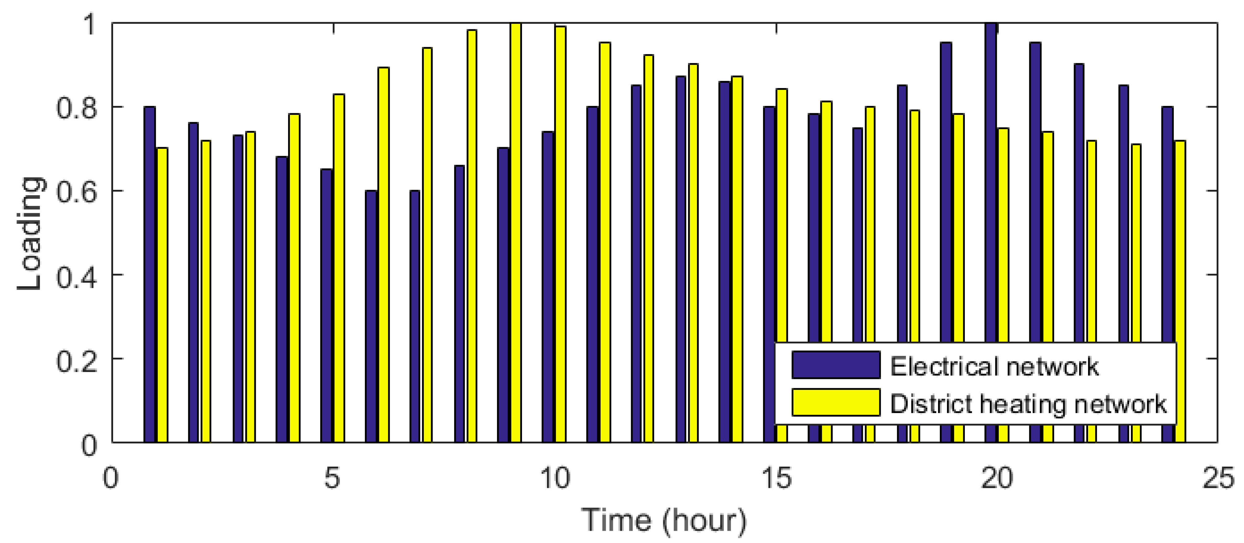
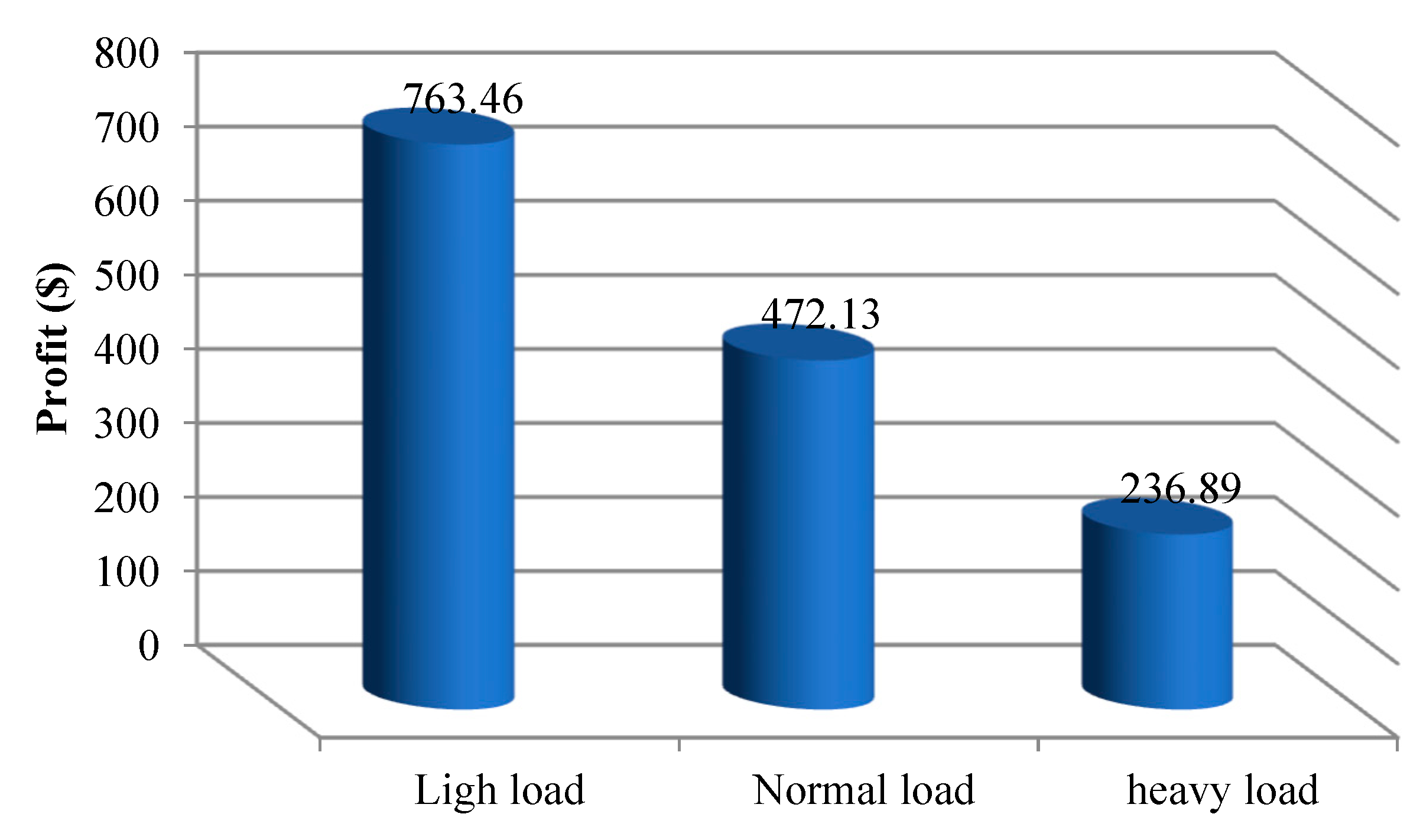
4.2.3. Impact of Different Loading Conditions

In this section, the energy profit has been evaluated by considering different load levels; i.e., low load, normal load, and high load, equivalent to 80%, 100%, and 120% of peak load, respectively. The results of the profit evaluation of EH considering different load levels are presented in Figure 12. As can be seen, with a 20% increase in the demand compared to the base state, the profit has decreased from $472.13 to $236.89, and with a 20% decrease in load demand, it has increased to $763.46. Therefore, the increase (decrease) in the load demand causes a decrease (increase) in the profit of the EH.

4.2.4. Impact of Forced Outage Rate

In this section, the energy profit is examined by considering the effect of the equipment-forced outage rate (FOR). The results of evaluating the profit of EH, taking into account the FOR of renewable energy sources and CHP equipment, are presented in

Table 6. Energy profit considering the FOR changes.

FOR	Profit ($)
0%	472.13
1%	445.43
2%	428.92
3%	412.43
4%	395.94
5%	379.46
6%	362.98
7%	346.51
8%	330.03
9%	313.56
10%	297.09

. As we know, the production capacity of resources depends on their availability and probability of functioning in healthy working conditions. Anticipated or anticipated failure of equipment for any reason reduces its availability in the system. In the previous simulations and for the base case, the FOR of renewable energy resources and CHP equipment was considered to be zero, or the probability of their operation was considered 100%. In this section, the energy profit of the system is calculated for FOR from 0% to 10% according to Table 6. It can be seen that with the increase (decrease) in the FOR of renewable energy sources and CHP, the profit of the hub has decreased (increased). For example, the profit of the system in the base state (FOR = 0%) has decreased from $472.13 to $379.46 for FOR = 5%, and has also declined to $297.09 for FOR = 10%.

5. Conclusions

The present paper addresses the optimal scheduling and management of EHs in day-ahead energy markets for participation with EGHNs to maximize energy profit using the new IFLA algorithm and satisfying the operating and hub constraints. The research findings are listed below:

• The results showed that the IFLA, FLA, PSO, and MRFO methods obtained energy profits of $472.13, $435.34, $442.17, and $467.62, respectively, in the day-ahead market, which indicates the better performance of the proposed framework based on IFLA in achieving more energy profit.
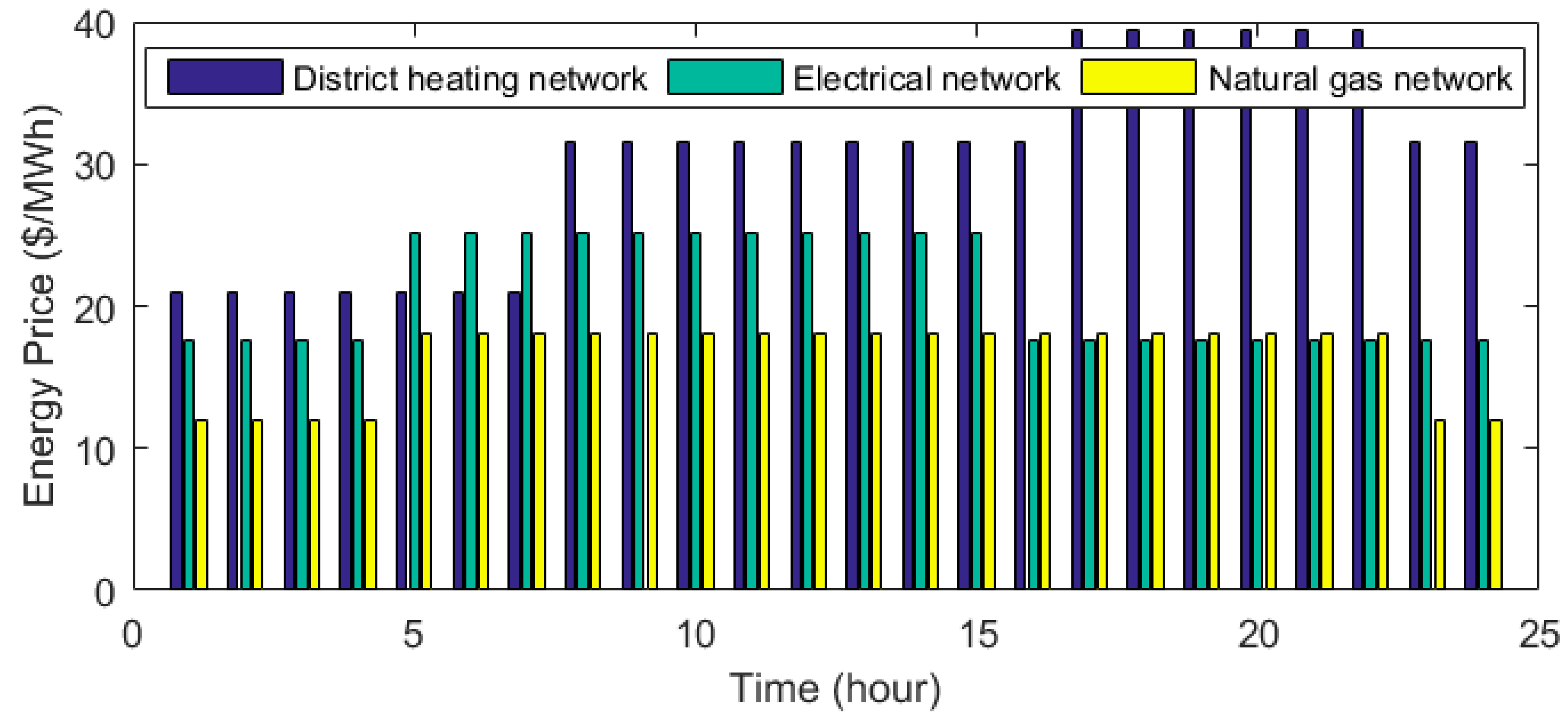
• The system’s profit is significantly affected by the price of electricity, natural gas, and heating energy. The profit of the heating market of the day-ahead is negative in the hours of electric energy storage and positive in the rest of the hours. Furthermore, the profit of the day-ahead gas market in the day-ahead heating market is negative compared to the day-ahead gas.
• With a 20% increase in load demand compared to the base state, the profit decreases from $472.13 to $236.89, and with a 20% decrease in load demand, it increases to $763.46. Therefore, the increase (decrease) in load demand causes a decrease (increase) in the profitability of the EH.
• With the increase (decrease) in the FOR of renewable energy sources and CHP, the system profit decreases (increases). The system profit in the base state (FOR = 0%) decreases from $472.13 to $379.46 for FOR = 5%, and also declines to $297.09 for FOR = 10%.

References

1. Mohammadi, M.; Noorollahi, Y.; Mohammadi-Ivatloo, B.; Yousefi, H. Energy hub: From a model to a concept–A review. Renew. Sustain. Energy Rev. 2017, 80, 1512–1527. [Google Scholar] [CrossRef]
2. Naderipour, A.; Kamyab, H.; Klemeš, J.J.; Ebrahimi, R.; Chelliapan, S.; Nowdeh, S.A.; Abdullah, A.; Marzbali, M.H. Optimal design of hybrid grid-connected photovoltaic/wind/battery sustainable energy system improving reliability, cost and emission. Energy 2022, 257, 124679. [Google Scholar] [CrossRef]
3. Davatgaran, V.; Saniei, M.; Mortazavi, S.S. Optimal bidding strategy for an energy hub in energy market. Energy 2018, 148, 482–493. [Google Scholar] [CrossRef]
4. Zhang, G.; Ge, Y.; Ye, Z.; Al-Bahrani, M. Multi-objective planning of energy hub on economic aspects and resources with heat and power sources, energizable, electric vehicle and hydrogen storage system due to uncertainties and demand response. J. Energy Storage. 2023, 57, 106160. [Google Scholar] [CrossRef]
5. Naderipour, A.; Abdul-Malek, Z.; Arabi Nowdeh, S.; Gandoman, F.H.; Hadidian Moghaddam, M.J. A multi-objective optimization problem for optimal site selection of wind turbines for reduce losses and improve voltage profile of distribution grids. Energies 2019, 12, 2621. [Google Scholar] [CrossRef] [Green Version]
6. Lu, X.; Li, H.; Zhou, K.; Yang, S. Optimal load dispatch of energy hub considering uncertainties of renewable energy and demand response. Energy 2023, 262, 125564. [Google Scholar] [CrossRef]
7. Naderipour, A.; Abdul-Malek, Z.; Nowdeh, S.A.; Ramachandaramurthy, V.K.; Kalam, A.; Guerrero, J.M. Optimal allocation for combined heat and power system with respect to maximum allowable capacity for reduced losses and improved voltage profile and reliability of microgrids considering loading condition. Energy 2020, 196, 117124. [Google Scholar] [CrossRef]
8. Wen, P.; Xie, Y.; Huo, L.; Tohidi, A. Optimal and stochastic performance of an energy hub-based microgrid consisting of a solar-powered compressed-air energy storage system and cooling storage system by modified grasshopper optimization algorithm. Int. J. Hydrog. Energy 2022, 47, 13351–13370. [Google Scholar] [CrossRef]
9. Bahmani, R.; Karimi, H.; Jadid, S. Cooperative energy management of multi-energy hub systems considering demand response programs and ice storage. Int. J. Electr. Power Energy Syst. 2021, 130, 106904. [Google Scholar] [CrossRef]
10. Rahmatian, M.R.; Shamim, A.G.; Bahramara, S. Optimal operation of the energy hubs in the islanded multi-carrier energy system using Cournot model. Appl. Therm. Eng. 2021, 191, 116837. [Google Scholar] [CrossRef]
11. Ghanbari, A.; Karimi, H.; Jadid, S. Optimal planning and operation of multi-carrier networked microgrids considering multi-energy hubs in distribution networks. Energy 2020, 204, 117936. [Google Scholar] [CrossRef]
12. Wang, X.; Liu, Y.; Liu, C.; Liu, J. Coordinating energy management for multiple energy hubs: From a transaction perspective. Int. J. Electr. Power Energy Syst. 2020, 121, 106060. [Google Scholar] [CrossRef]
13. Mirzapour-Kamanaj, A.; Majidi, M.; Zare, K.; Kazemzadeh, R. Optimal strategic coordination of distribution networks and interconnected energy hubs: A linear multi-follower bi-level optimization model. Int. J. Electr. Power Energy Syst. 2020, 119, 105925. [Google Scholar] [CrossRef]
14. Liu, T.; Zhang, D.; Wu, T. Standardised modelling and optimisation of a system of interconnected energy hubs considering multiple energies—Electricity, gas, heating, and cooling. Energy Convers. Manag. 2020, 205, 112410. [Google Scholar] [CrossRef]
15. Khorasany, M.; Najafi-Ghalelou, A.; Razzaghi, R.; Mohammadi-Ivatloo, B. Transactive energy framework for optimal energy management of multi-carrier energy hubs under local electrical, thermal, and cooling market constraints. Int. J. Electr. Power Energy Syst. 2021, 129, 106803. [Google Scholar] [CrossRef]
16. Mohammadi, M.; Noorollahi, Y.; Mohammadi-ivatloo, B.; Hosseinzadeh, M.; Yousefi, H.; Khorasani, S.T. Optimal management of energy hubs and smart energy hubs—A review. Renew. Sustain. Energy Rev. 2018, 89, 33–50. [Google Scholar] [CrossRef]
17. Huo, D.; Le Blond, S.; Gu, C.; Wei, W.; Yu, D. Optimal operation of interconnected energy hubs by using decomposed hybrid particle swarm and interior-point approach. Int. J. Electr. Power Energy Syst. 2018, 95, 36–46. [Google Scholar] [CrossRef]
18. Bostan, A.; Nazar, M.S.; Shafie-Khah, M.; Catalão, J.P. Optimal scheduling of distribution systems considering multiple downward energy hubs and demand response programs. Energy 2020, 190, 116349. [Google Scholar] [CrossRef]
19. Luo, X.; Liu, Y.; Liu, J.; Liu, X. Energy scheduling for a three-level integrated energy system based on energy hub models: A hierarchical Stackelberg game approach. Sustain. Cities Soc. 2020, 52, 101814. [Google Scholar] [CrossRef]
20. Zhang, X.; Che, L.; Shahidehpour, M.; Alabdulwahab, A.S.; Abusorrah, A. Reliability-based optimal planning of electricity and natural gas interconnections for multiple energy hubs. IEEE Trans. Smart Grid 2015, 8, 1658–1667. [Google Scholar] [CrossRef]
21. Ghorab, M. Energy hubs optimization for smart energy network system to minimize economic and environmental impact at Canadian community. Appl. Therm. Eng. 2019, 151, 214–230. [Google Scholar] [CrossRef]
22. Gholinejad, H.R.; Loni, A.; Adabi, J.; Marzband, M. A hierarchical energy management system for multiple home energy hubs in neighborhood grids. J. Build. Eng. 2020, 28, 101028. [Google Scholar] [CrossRef]
23. Jiang, W.; Wang, X.; Huang, H.; Zhang, D.; Ghadimi, N. Optimal economic scheduling of microgrids considering renewable energy sources based on energy hub model using demand response and improved water wave optimization algorithm. J. Energy Storage 2022, 55, 105311. [Google Scholar] [CrossRef]
24. Shahrabi, E.; Hakimi, S.M.; Hasankhani, A.; Derakhshan, G.; Abdi, B. Developing optimal energy management of energy hub in the presence of stochastic renewable energy resources. Sustain. Energy Grids Netw. 2021, 26, 100428. [Google Scholar] [CrossRef]
25. Enayati, M.; Derakhshan, G.; mehdi Hakimi, S. Optimal energy scheduling of storage-based residential energy hub considering smart participation of demand side. J. Energy Storage 2022, 49, 104062. [Google Scholar] [CrossRef]
26. Lu, Q.; Zeng, W.; Guo, Q.; Lü, S. Optimal operation scheduling of household energy hub: A multi-objective optimization model considering integrated demand response. Energy Rep. 2022, 8, 15173–15188. [Google Scholar] [CrossRef]
27. AkbaiZadeh, M.; Niknam, T.; Kavousi-Fard, A. Adaptive robust optimization for the energy management of the grid-connected energy hubs based on hybrid meta-heuristic algorithm. Energy 2021, 235, 121171. [Google Scholar] [CrossRef]
28. Wolpert, D.H.; Macready, W.G. No free lunch theorems for optimization. IEEE Trans. Evol. Comput. 1997, 1, 67–82. [Google Scholar] [CrossRef] [Green Version]
29. Hashim, F.A.; Mostafa, R.R.; Hussien, A.G.; Mirjalili, S.; Sallam, K.M. Fick’s Law Algorithm: A physical law-based algorithm for numerical optimization. Knowl.-Based Syst. 2023, 260, 110146. [Google Scholar] [CrossRef]
30. Abualigah, L.; Diabat, A.; Zitar, R.A. Orthogonal Learning Rosenbrock’s Direct Rotation with the Gazelle Optimization Algorithm for Global Optimization. Mathematics 2022, 10, 4509. [Google Scholar] [CrossRef]
31. Shabanpour-Haghighi, A.; Seifi, A.R. Simultaneous integrated optimal energy flow of electricity, gas, and heat. Energy Convers. Manag. 2015, 101, 579–591. [Google Scholar] [CrossRef]
32. Kennedy, J.; Eberhart, R. Particle swarm optimization. In Proceedings of the Name of ICNN’95-International Conference on Neural Networks, Perth, WA, Australia, 27 November–1 December 1995; Volume 4, pp. 1942–1948. [Google Scholar]
33. Zhao, W.; Zhang, Z.; Wang, L. Manta ray foraging optimization: An effective bio-inspired optimizer for engineering applications. Eng. Appl. Artif. Intell. 2020, 87, 103300. [Google Scholar] [CrossRef]
34. Kohansal, O.; Zadehbagheri, M.; Kiani, M.J.; Nejatian, S. Participation of Grid-Connected Energy Hubs and Energy Distribution Companies in the Day-Ahead Energy Wholesale and Retail Markets Constrained to Network Operation Indices. Int. Trans. Electr. Energy Syst. 2022, 2022, 2463003. [Google Scholar] [CrossRef]
Figure 1. The presented framework of optimal energy scheduling of the EH.
Applsci 13 03526 g001
Figure 2. Schematic of the studied system.
Applsci 13 03526 g002
Figure 3. The daily curve of network load percentage [31].
Applsci 13 03526 g003
Figure 4. The daily curve of energy prices in the DA market [31,34].
Applsci 13 03526 g004
Figure 5. The daily curve of irradiance.
Applsci 13 03526 g005
Figure 6. The daily curve of wind speed.
Applsci 13 03526 g006
Figure 7. Convergence behavior of various algorithms when applied to solve the problem.
Applsci 13 03526 g007
Figure 8. Daily changes of hub power for different energy equipment.
Applsci 13 03526 g008
Figure 9. Daily changes in the profit hub.
Applsci 13 03526 g009
Figure 10. Daily power loss curve in EGHNs.
Applsci 13 03526 g010
Figure 11. Maximum daily variations in voltage, pressure, and temperature curves.
Applsci 13 03526 g011
Figure 12. Energy profit considering different load levels.
Applsci 13 03526 g012