Abstract
Back focal plane (BFP) ellipsometry, which acquires the ellipsometric parameters of reflected light at different incident and azimuthal angles through a high-NA objective lens, has recently shown great potential in industrial film measurement. In on-line metrology cases for film manufacturing, the film vibration, which is caused by equipment vibrations or environmental disturbances, results in defocus blur and distortion of the received BFP images. Thus, subsequently extracted ellipsometric spectra and film parameters significantly deviate from the ground truth values. This paper proposes a cost-effective method for correcting vibration-induced BFP ellipsometric spectral errors. The method relies on an initial incident angle calibration of BFP radii at different defocus positions. Then, corresponding ellipsometric spectral errors are corrected by inserting a calibrated Jones compensation matrix into a system model. During measurement, the defocus position of the vibrational film is first determined. Then, BFP ellipsometric spectral errors, including incident angle mapping distortion and ellipsometric parameter variations, are corrected for a bias-free film analysis using the previous calibration results. Experimental results showed that this method significantly improved measurement accuracy without vibrational defocus compensation, from over 30 nm down to less than 1 nm.
1. Introduction
Thin films play an essential role in manufacturing semiconductors and display electronics. The thicknesses and refractive indices of thin films should be well controlled and measured for production efficiency improvement and yield control [1,2]. Among the various thin-film sensing technologies [3,4,5,6], ellipsometry is widely used due to its ability to carry out rapid, nondestructive, and high-precision measurement [7,8,9,10,11]. In recent times, ellipsometry has also been widely used in surface and interface measurement and characterization of nanostructures and optoelectronic materials [12,13,14]. Ellipsometric measurements depend on a mechanical system called a goniometer. Any vibration results in signal distortion problems in the ellipsometric measurements and consequent variation in the optical parameters of the investigated film [15,16,17]. The signal distortion problems resulting from the vibration are especially significant in on-line inspection cases using rotating compensator ellipsometry. Specifically, the signals of an ellipsometer captured at different times may have different errors or distortions due to the varying defocus distances caused by vibrations, making it difficult to characterize errors of subsequent thin-film parameter calculation. Therefore, a method to overcome vibration-induced measurement distortion in on-line inspection of thin films is urgently needed.
Back focal plane ellipsometry (also known as angle-resolved ellipsometry or microellipsometry) [18,19,20,21] has advantages in overcoming the challenges of conventional ellipsometry in defocused measurements under vertical vibrations (vertical vibration defocus is simply referred to as defocus from hereon) due to its fast measurement characteristics based on a single-frame BFP imaging and equivalent sensitivity to conventional ellipsometry. This method can obtain single-frame BFP reflectance and ellipsometric information of different incident and azimuth angles through a high-NA (numerical aperture) objective lens without using mechanical moving parts to realize angular or spectral scanning. Moreover, single-frame BFP images can also easily process defocus effects in real time. Compared to the inclined structure of conventional ellipsometry, the coaxial structure of BFP ellipsometry is spatially compact for on-line measurements and suffers from a smaller influence of defocused structures [22]. Different methods of improvement have been developed for single-frame BFP ellipsometry, e.g., modeling using the Mueller matrix [23], introducing compensator modulations [24,25], capturing through a color camera [20], and applying on-line measurement of oil film gaps [26,27]. However, in BFP ellipsometric measurement, when vibrational defocus occurs, the captured BFP images may suffer from blur and distortion, resulting in the distortion of incident angles and incorrect ellipsometric responses. This issue has not been analyzed and solved. Suppose an incident angle distortion and the corresponding ellipsometric error are calibrated at each defocus position. In that case, the BFP accuracy could be improved by compensating the errors related to the defocus effect in the single-frame measurement model [28,29,30].
This work proposes an effective calibration and compensation method for sample vibration-induced defocus effect in BFP ellipsometry. The method begins by calibrating defocus-induced incident angle distortion using the Brewster angle of a standard material. Then, the ellipsometric errors are corrected by inserting a calibrated compensation matrix into a system model using a Jones matrix. During actual measurement, the defocus position is determined by analyzing the frequency domain and energy characteristics of a BFP image. Then, the previous calibration results compensate for incident angle distortion and ellipsometric errors. Several thin-film validation experiments were carried out, which verified that the method significantly improved the film thickness measurement accuracy of BFP ellipsometry.
2. Method
2.1. Hardware Configuration
Figure 1a shows the layout and configuration of the BFP ellipsometry measurement system, which includes four parts: an illumination light source, a measurement probe, a detection unit, and a motorized positioning unit. The white light generated by a halogen lamp is collimated, then passes through a band-pass filter and becomes monochromatic (@632.8 nm). A diaphragm is used to control the beam radius. The monochromatic light becomes linearly polarized after passing through a polarizer and is reflected by a beam splitter before becoming incident on the sample through a high-NA objective lens at different incident angles. Then, the reflected light is recollected by the objective and focused on the BFP. After passing through the beam splitter and an analyzer, the BFP image is captured by a CMOS, as shown in Figure 1d. The motorized positioning unit uses a motorized translation stage to hold the sample and simulates the defocus of the sample generated by vertical vibration at different positions.

Figure 1.
The measurement principle of BFP ellipsometry: (a) hardware configuration; (b) polarization change of incident and reflected beams denoted in blue and red, respectively; (c) the relationship between the BFP radius R and incident angle θ; (d) the BFP image of a SiO2 film.
2.2. BFP Ellipsometry Principle
In a BFP ellipsometry system, the state of polarization of the incident light changes with the azimuthal angle on a BFP due to the high-NA objective lens. This incident plane rotating effect plays the role of a rotating polarizer, just like a typical rotating polarizer ellipsometer. Therefore, the annular intensity for any radius of the back focal plane is a function of the azimuthal angle. The ellipsometric parameters of the measured sample can thus be calculated by fitting the measured annular intensity to the optical model.
As shown in Figure 1b,c, every radius of the BFP R is mapped to a unique incident angle θ. The angular range is determined by the NA of the objective lens, from to . The measurement system can be modeled by the Jones matrix method, e.g.,
where Ein and Eout are the input and output complex electric fields, respectively; ,, and are the Jones matrices of the sample, analyzer, and polarizer, respectively; and R is the coordinate rotation matrix. JM is the reflection matrix redirected to the reference X-axis, and φ is the azimuth angle. P and A represent the angle of the transmittance axis of the polarizer and analyzer concerning the X-axis. By setting the polarizer and analyzer at 0 and 45 degrees, respectively, the received intensity of the captured BFP image can be expressed as follows:
where the three coefficients are the zero-, second-, and fourth-order Fourier coefficients of (φ), respectively, and are the intermediate important quantities for solving subsequent parameters. For these three important intermediate Fourier coefficients, they can be easily extracted using the traditional Fourier transform. Further, the angle-resolved ellipsometric parameters (Ψ(θ) and Δ(θ)) can be calculated from the three coefficients using Equations (3) and (4):
Subsequently, the film parameters can be determined by fitting the measured angle-resolved spectra to the theoretical model with nonlinear multivariate regression using the Levenberg–Marquardt (LM) algorithm [31]. The merit function is as follows:
where the subscripts “exp” and “the” represent the measured and theoretical values, respectively.
3. Defocus Effect Calibration and Compensation
3.1. Defocused BFP Incident Angle Calibration
In the proposed method, the relationship between BFP image radius R and incident angle θ must be accurately calibrated at each defocus position. According to Abbe’s sine condition [32], the relationship between θ and R can be expressed as . Choi [20] built the relationship assisted by the NA of the objective lens and Rmax of the BFP image. However, Rmax varies with the defocus position for blur and distortion, as shown in Figure 2. Therefore, the angle distortion happens at defocus positions where Rmax no longer corresponds to NA, and the mapping relationship is distorted.
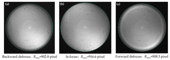
Figure 2.
Maximum BFP image radii of a 44.34 nm SiO2 film at different defocus positions and its blurring and distortion: (a) a backward-defocused BFP image near the objective lens; (b) an in-focus BFP image; (c) a forward-defocused BFP image far from the objective lens.
A full-field Brewster angle method is proposed to deal with the defocused calibration problem. The method stems from the fact that the position of minimum p-polarized reflectance corresponds to the Brewster angle. In our previous study [21], the ellipsometric amplitude ratio Ψ(θ) was demonstrated to be more robust in searching for the position of the Brewster angles than the reflectance intensities. We begin by calculating the angle-resolved ellipsometric parameter Ψ(θ) at the BFP of a boundary reflection and then searching for the Brewster angle θB corresponded BFP radius RB. Here, a local quadratic polynomial fitting determines the pixel radius RB of Ψ(θ)min. Thus, the relationship between θ and R is built using Equation (6):
where is the refractive index of air, is the refractive index of the standard sample, and f’ is a mapping coefficient in the Brewster angle calibration.
In order to obtain the boundary reflection for searching θB, the light transmitted into the medium needs to be completely absorbed or filtered away. For this purpose, a thick transparent plate is normally used, where large-angle light of reflection from the backside can be spatially eliminated. Considering the limitation of NA (0.9) of the objective lens, θB of a selected standard sample should be within the limited range of the objective lens. Therefore, a thick K9 glass plate was chosen as the standard sample to calibrate the incident angle distortion due to the limited focal depth and because the NA of the used objective lens and the reflected light from the backside of a thick film reflects away from the detection unit. During the calibration process, the angle-resolved Ψ of each defocused BFP image was first calculated with Equation (3). Then, the pixel radius RB corresponding to the Brewster angle at different defocus positions was fitted. Further, the calibration coefficient f’ was calculated at different defocus positions with Equation (6). From a set of Brewster angle mapping coefficients calibrated at different defocus positions, an R–θ mapping function could then be built at a specific defocus position. Using this, a defocused BFP ellipsometric spectrum can be turned to be distortion-free in an incident angle domain.
3.2. Defocused BFP Ellipsometric Error Calibration
Vibrational defocus causes BFP images to blur and distort and results in abnormal optical ellipsometric responses, e.g., Ψ and Δ. As shown in Figure 3, the errors of Ψ and Δ increase as the defocus distance increases regularly. Obviously, it is crucially important to correct this error once a sample is defocused. The ellipsometric parameter errors have been investigated by Linke et al. [22,33], following which a Jones matrix of was used to model the ellipsometric parameter errors resulting from the defocus from an objective lens in this study. In the coaxial path system, the objective polarization errors are considered twice, corresponding to emission and reflection through the objective lens. Thus, a complete error model from a measured sample can be described as , where and are the ellipsometric compensation’s amplitude and phase parameters, respectively. The calibration of and can be achieved using some reference materials through Equation (7) based on the least square error fitting:

Figure 3.
Comparison of the standard 44.34 nm SiO2 film measured ellipsometric parameters at different defocus positions: (a) Ψ and (b) Δ; the black dashed lines represent the ellipsometric parameter of the theory.
The method of calibration has no special requirement for the standard thin film sample except isotropy. Any isotropic standard thin film samples can be used in the calibration.
By observing a reference material at different defocus positions and fitting through Equation (7), a two-dimensional compensation look-up table of Ψ and Δ could be made on a – domain. In the actual measurement, the ellipsometric compensations and are found from the look-up table by determining the defocus position. Film parameters can then be calculated through LM fitting using the merit function in Equation (7).
3.3. Defocus Position Determination and Defocus Effect Compensation
As mentioned above, both the incident angle calibration and ellipsometric parameter compensation rely on the accurate determination of defocus distance of a film. A defocus determination method based on actual BFP image characterization is introduced. The frequency domain analysis method, generally applied in autofocusing [34,35], stems from the imaging resolution varying with defocus. The high-frequency signal in the image spectrum will be lost due to blurring when defocus occurs. In other words, the high-frequency components of a BFP image reduce when defocusing. This fact can establish the relationship between the frequency domain evaluation function of a defocused BFP image and its defocus position . The method begins with a discrete Fourier transform (DFT), and the formula of DFT for M × N digital image is shown in Equation (8):
where k and l are frequency domain pixel coordinates, and μ and ν are image pixel coordinates. The spectrum function Ps denoting the pixel intensity of the image is shown in Equation (9) below:
Thus, the frequency domain transform evaluation function F based on DFT is obtained as shown in Equation (10):
The relationship between the evaluation function F and defocus position is shown in Figure 4a. The negative values of indicate a defocus direction away from the objective lens, while the positive values indicate towards the objective lens. The determination criterion from the F curve shows high resolution and sensitivity in the defocus position around [–35,45] μm (bold solid red line), which is very suitable for calculating the defocus position of the defocus sample near the focal point. However, the resolution and sensitivity of the far focus position are significantly reduced, as shown by the dotted line in Figure 4a. Moreover, the curve is convex and cannot tell the defocus direction.
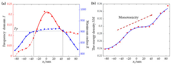
Figure 4.
Three different evaluation function were sampled from an experiment regarding defocus positions (curves represent a polynomial fit): (a) the frequency domain method using normalized DFT and the maximum radius method (the dashed lines corresponding to high sensitivity is used as the criteria for defocus determination); (b) the energy density method.
Therefore, considering that the size of the imaging spot on the BFP changes with the defocus position, the maximum radius method and energy density method are introduced to overcome the limitation of the frequency domain method in calculating the defocus position . The maximum radius method extracts the Rmax of the BFP image through edge detection, and the obtained Rmax- curve shows high resolution and sensitivity in the far-end focus positions (less than −35 μm and more than 45 μm), as shown by the blue line in Figure 4a, where Fp is a threshold used to distinguish the high resolution and sensitivity of the defocus position curve from the low resolution and sensitivity. Further, a combination of the maximum radius method and frequency domain method shows significant improvement in calculating the defocus amount accurately, but the defocus direction remains to be determined. To address this problem, we introduced an energy density method. This method calculates the energy density within the Rmax of a BFP image using , where Smax is the pixel area of the circle with a radius of Rmax, and is the sum of intensity values of image pixels within Rmax. An experimental variation curve of the energy density regarding defocus positions is shown in Figure 4b. It shows favorable monotonicity in defocusing direction determination.
To sum up, a high-sensitivity determination algorithm combined using the above three defocus evaluation indicators is proposed. The working process of the proposed algorithm is as follows. Firstly, the frequency domain evaluation values F, maximum radii R, and energy density NM are calculated from a BFP image. Since the F– curve is divided into a high-sensitivity part and a less-sensitive part by the threshold value Fp. When F is less than Fp, the maximum radius method is used to calculate the defocus position based on the Rmax curve; otherwise, the frequency domain method is adopted. Two solutions exist: and . The nonmonotonicity is then determined by comparing NM1 and NM2. The algorithm flow chart is shown in Figure 5. The threshold Fp used to determine the defocus position calculation can be determined according to the position where the gradient of the frequency standard curve drops sharply, as shown in Figure 4a. Determining the position of the defocus BFP image according to the above process provides a key link for the defocus BPF image compensation and a basis for subsequent defocus measurement.

Figure 5.
Flow chart of the proposed defocus position determination algorithm.
A complete BFP image undistortion and ellipsometric error compensation example is shown in Figure 6a using the proposed method. Firstly, the original biased ellipsometric parameters corresponding to each pixel radius were calculated, as shown in Figure 6b, using Equations (3) and (4). Then, based on a calculated defocus position, the incident angle calibration coefficient f’ and the ellipsometric compensation amounts and were determined from the previous calibration results, using which the R–θ correction and ellipsometric parameter compensation were completed, as shown in Figure 6c. Finally, the film thickness was further calculated using LM fitting.
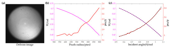
Figure 6.
A defocus-effect correction example of the proposed BFP ellipsometry: (a) a defocus BFP image of SiO2 film; (b) directly obtained ellipsometric parameters; (c) theoretical and measured value after incident angle calibration and compensation of the ellipsometric parameters; black lines represent the theoretical values and colorful lines represent the measured values after correction.
4. Experiment and Results
4.1. Experimental Setup
By comparing with some existing optical measurement systems, this system’s light source was a broadband halogen lamp (OSL2 from Thorlabs), and a laser line filter (FL632.8-1, Thorlabs) created quasi-monochromatic light with a central wavelength of 632.8 nm. The collimating and the imaging lens used were achromatic. The polarizer and analyzer were Glan–Taylor polarizers (PGT6315, Joint Optics), and the objective lens of NA 0.9 from Olympus (semidecolorizer, 100×) were used. As for the detector, an MER-500 CMOS camera was used. The sample was clamped on an electric displacement table (model Zolix-CXP15-40) with a minimum step distance of 5 μm.
4.2. Calibration and Compensation Results
The following steps were carried out: incident angle distortion calibration, ellipsometric compensation amount calibration, and defocus position curve calibration.
Firstly, the defocused incident angle distortion was calibrated based on the Brewster angle calibration method described in Section 3.1. A thick K9 glass plate sample with a refractive index of 1.1515 (with a Brewster angle of θB = 56.57°) was selected as the calibration material. We used an electric positioning stage to obtain defocused BFP images with a 10 μm interval at different defocus positions . The corresponding pixel radii of the Brewster angle RB at different defocus positions were then extracted. After that, the mapping function of the Brewster angle radii of defocus positions was obtained using a polynomial fitting, as shown in Figure 7b. With the calibrated Brewster angle radius curve, defocus-resulted incident angle distortion could be corrected using Equation (6).
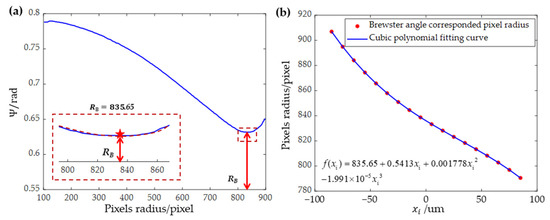
Figure 7.
Incident angle calibration experiment with a standard thick K9 glass plate: (a) the calculated angle-resolved Ψ and Ψmin corresponding to pixel radius RB; (b) the relationship between Brewster angle corresponding to pixel radius RB of defocus position .
Secondly, the defocused ellipsometric parameter errors, including and , were calibrated. A SiO2 film sample with a thickness of 45 nm (nominal thickness) grown on a Si substrate was used for the calibration. An electric stage was used to simulate the defocus behaviors for BFP image acquisition within a ± 85 μm defocus range with an interval of 5 μm (the range in the actual film manufacturing process was within ±50 μm near a roller). After calculating the experimental angular ellipsometric spectra at a defocus position using Equations (3) and (4), the ellipsometric compensation amount of and at each incident angle was estimated through Equation (7). Repeating the compensation calibration at each defocus position resulted in a two-dimensional compensation map on a domain of –, which was finally interpolated for subsequent compensation measurement. Figure 8 shows the interpolated compensation maps of the ellipsometric parameters.
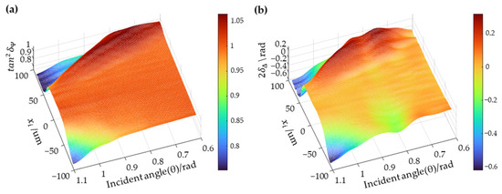
Figure 8.
Calibrated ellipsometric maps of compensation (a) and (b) from a SiO2 film.
Finally, the maximum radius R, the frequency domain function value F, and the energy density NM of the 37 defocused BFP images were calculated for real-time defocus position determination, as shown in Figure 4.
4.3. Experimental Results
In the verification experiments, three SiO2 films (Si substrate) with different thicknesses (25, 45, and 100 nm) were measured by acquiring BFP images at 20 defocus positions using a positioning stage with an interval of 10 μm. Multiple images were collected at the same defocus position for repeatability analysis. The ellipsometric parameters and of the defocus image were calculated according to an estimated defocus position using the method shown in Section 3.3. Then, the ellipsometric compensation amounts and were obtained by referring to the compensation maps at the corresponding defocus position. Film thickness was finally calculated by fitting using the LM algorithm. Simultaneously, film thickness was also calculated from the original BFP images without vibrational compensation. All the obtained film thickness results are presented in Figure 9.

Figure 9.
SiO2 film thickness measurement experiments using the proposed method: (a) results of a film with nominal thickness of 25 nm; (b) results of a nominal thickness of 45 nm; (c) results of a nominal thickness of 100 nm; and (d) absolute thickness errors of the three thin films.
The experimental results showed that the measurement accuracy was significantly improved by correcting the defocused BFP images using the proposed method. Compared to the case without vibration defocus compensation, this method significantly improved the measurement accuracy of thin film, from more than 30 nm to less than 1 nm.
5. Conclusions
This paper proposes a cost-effective method for correcting vibration-induced BFP ellipsometric spectral errors. The method first calibrates the defocused incident angle distortion using the Brewster angle of reference material. Then, an ellipsometric compensation amount is inserted into the system model as a Jones matrix to correct the error of the ellipsometric parameters at different defocus positions. Moreover, the defocus position of an actual BFP image is determined by analyzing its frequency domain and energy characteristics. Once the defocus position of a BFP image is calculated, the corresponding incident angle distortion can be corrected, and the ellipsometric errors can be compensated using the previous calibration results. Our experiments showed that the absolute error of the measurement reduced from over 30 nm down to less than 1 nm, within a defocused range of ±85 μm. As the compensation completes every single frame of the BFP image, the method is expected to be applied for on-line BFP ellipsometry under vibration conditions.
In the future, the defocus measurement method can be improved from three aspects. Firstly, the method needs to be demonstrated in real-time vibrational environments. Secondly, a monotonic defocus position determination method with better resolution and sensitivity needs to be developed. Third, antivibrational methods for general spectral ellipsometry, such as wavelength scanning BFP ellipsometry, need to be developed.
Author Contributions
Conceptualization, methods, comments, verification, J.W., L.P. and D.T.; investigation and issuing letters of credit, F.G., R.C. and L.Z.; writing—first draft preparation, J.Y. and J.W. All authors have read and agreed to the published version of the manuscript.
Funding
This research was supported by the National Natural Science Foundation of China (No. 52075206, 51835005) and the Key R&D Program of Hubei Province (2021BAA056).
Institutional Review Board Statement
Not applicable.
Informed Consent Statement
Not applicable.
Data Availability Statement
Data underlying the results presented in this paper are not publicly available at this time but may be obtained from the authors upon reasonable request.
Conflicts of Interest
The authors declare no conflict of interest.
References
- Lee, S.W.; Choi, G.; Lee, S.Y.; Cho, Y.; Pahk, H.J. Coaxial Spectroscopic Imaging Ellipsometry for Volumetric Thickness Measurement. Appl. Opt. 2021, 60, 67–74. [Google Scholar] [CrossRef] [PubMed]
- Lee, S.W.; Lee, S.Y.; Choi, G.; Pahk, H.J. Co-Axial Spectroscopic Snap-Shot Ellipsometry for Real-Time Thickness Measurements with a Small Spot Size. Opt. Express 2020, 28, 25879–25893. [Google Scholar] [CrossRef] [PubMed]
- Ghim, Y.S.; Rhee, H.G. Instantaneous Thickness Measurement of Multilayer Films by Single-Shot Angle-Resolved Spectral Reflectometry. Opt. Lett. 2019, 44, 5418–5421. [Google Scholar] [CrossRef] [PubMed]
- Guo, T.; Yuan, L.; Tang, D.; Chen, Z.; Gao, F.; Jiang, X. Analysis of the Synchronous Phase-Shifting Method in a White-Light Spectral Interferometer. Appl. Opt. 2020, 59, 2983–2991. [Google Scholar] [CrossRef]
- Miao, Z.; Tang, Y.; Wei, K.; Zhang, Y. Optimization of Stepping Mueller Matrix Ellipsometer Configuration Based on Weighed Factor. Opt. Eng. 2022, 61, 044102. [Google Scholar] [CrossRef]
- Jiang, H.; Ma, Z.; Gu, H.; Chen, X.; Liu, S. Characterization of Volume Gratings Based on Distributed Dielectric Constant Model Using Mueller Matrix Ellipsometry. Appl. Sci. 2019, 9, 698. [Google Scholar] [CrossRef]
- Fujiwara, H. Spectroscopic Ellipsometry: Principles and Applications; John Wiley & Sons: Hoboken, NJ, USA, 2007. [Google Scholar]
- Finlayson, C.E.; Rosetta, G.; Tomes, J.J. Spectroscopic Ellipsometry and Optical Modelling of Structurally Colored Opaline Thin-Films. Appl. Sci. 2022, 12, 4888. [Google Scholar] [CrossRef]
- Liu, S.; Du, W.; Chen, X.; Jiang, H.; Zhang, C. Mueller Matrix Imaging Ellipsometry for Nanostructure Metrology. Opt. Express 2015, 23, 17316–17329. [Google Scholar] [CrossRef]
- Ohlídal, I.; Vohánka, J.; Buršíková, V.; Franta, D.; Čermák, M. Spectroscopic Ellipsometry of Inhomogeneous Thin Films Exhibiting Thickness Non-Uniformity and Transition Layers. Opt. Express 2019, 28, 160–174. [Google Scholar] [CrossRef]
- Stenzel, O.; Ohlídal, M. Optical Characterization of Thin Solid Films; Springer Series in Surface Sciences; Springer: Berlin/Heidelberg, Germany, 2018. [Google Scholar]
- Chen, C.; Chen, X.; Xia, Z.; Shi, J.; Sheng, S.; Qiao, W.; Liu, S. Characterization of Pixelated Nanogratings in 3D Holographic Display by an Imaging Mueller Matrix Ellipsometry. Opt. Lett. 2022, 47, 3580–3583. [Google Scholar] [CrossRef]
- Chen, X.; Gu, H.; Liu, J.; Chen, C.; Liu, S. Advanced Mueller Matrix Ellipsometry: Instrumentation and Emerging Applications. Sci. China Technol. Sci. 2022, 65, 2007–2030. [Google Scholar] [CrossRef]
- Fang, M.; Gu, H.; Guo, Z.; Liu, J.; Huang, L.; Liu, S. Temperature and Thickness Dependent Dielectric Functions of Mote2 Thin Films Investigated by Spectroscopic Ellipsometry. Appl. Surf. Sci. 2022, 605, 154813. [Google Scholar] [CrossRef]
- Aspnes, D.E. Spectroscopic Ellipsometry—Past, Present, and Future. Thin Solid Film. 2014, 571, 334–344. [Google Scholar] [CrossRef]
- Losurdo, M.; Bergmair, M.; Bruno, G.; Cattelan, D.; Cobet, C.; de Martino, A.; Fleischer, K.; Dohcevic-Mitrovic, Z.; Esser, N.; Galliet, M.; et al. Spectroscopic Ellipsometry and Polarimetry for Materials and Systems Analysis at the Nanometer Scale: State-of-the-Art, Potential, and Perspectives. J. Nanopart Res. 2009, 11, 1521–1554. [Google Scholar] [CrossRef] [PubMed]
- Likhachev, D.V. Efficient Thin-Film Stack Characterization Using Parametric Sensitivity Analysis for Spectroscopic Ellipsometry in Semiconductor Device Fabrication. Thin Solid Film. 2015, 589, 258–263. [Google Scholar] [CrossRef]
- Zhan, Q.; Leger, J. R Microellipsometer with Radial Symmetry. Appl. Opt. 2002, 41, 4630–4637. [Google Scholar] [CrossRef]
- Zhan, Q.; Leger, J.R. High-Resolution Imaging Ellipsometer. Appl. Opt. 2002, 41, 4443–4450. [Google Scholar] [CrossRef]
- Choi, G.; Lee, S.W.; Lee, S.Y.; Pahk, H.J. Single-Shot Multispectral Angle-Resolved Ellipsometry. Appl. Opt. 2020, 59, 6296–6303. [Google Scholar] [CrossRef] [PubMed]
- Peng, L.; Tang, D.; Wang, J.; Chen, R.; Gao, F.; Zhou, L. Robust Incident Angle Calibration of Angle-Resolved Ellipsometry for Thin Film Measurement. Appl. Opt. 2021, 60, 3971–3976. [Google Scholar] [CrossRef] [PubMed]
- Ye, S.H.; Kim, S.H.; Kwak, Y.K.; Cho, H.M.; Cho, Y.J.; Chegal, W. Angle-Resolved Annular Data Acquisition Method for Microellipsometry. Appl. Opt. 2007, 15, 56–65. [Google Scholar] [CrossRef] [PubMed]
- Fallet, C. Overlay Measurements by Mueller Polarimetry in Back Focal Plane. J. Micro Nanolithography MEMS MOEMS 2011, 10, 033017. [Google Scholar] [CrossRef]
- Otsuki, S.; Murase, N.; Kano, H. Back Focal Plane Microscopic Ellipsometer with Internal Reflection Geometry. Opt. Commun. 2013, 294, 24–28. [Google Scholar] [CrossRef]
- Otsuki, S.; Murase, N.; Kano, H. Mueller Matrix Microscopic Ellipsometer. Opt. Commun. 2013, 305, 194–200. [Google Scholar] [CrossRef]
- Namba, K.; Fukuzawa, K.; Itoh, S.; Zhang, H.; Azuma, N. Extension of Measurement Range of Lubrication Gap Shape Using Vertical-Objective-Type Ellipsometric Microscopy with Two Compensator Angles. Tribol. Int. 2020, 142, 105980. [Google Scholar] [CrossRef]
- Song, Y.; Fukuzawa, K.; Itoh, S.; Zhang, H.; Azuma, N. In-Situ Measurement of Temporal Changes in Thickness of Polymer Adsorbed Films from Lubricant Oil by Vertical-Objective-Based Ellipsometric Microscopy. Tribol. Int. 2022, 165, 107341. [Google Scholar] [CrossRef]
- Chen, L.; Wang, J.; Xu, M. Analysis and Calibration of Defocus Detection System based on Astigmatic Method. Laser Optoelectron. Prog. 2016, 53, 051205. [Google Scholar] [CrossRef]
- Zhao, X.; Suzuki, T.; Sasaki, O. Photothermal Phase-Modulating Laser Diode Interferometer with High-Speed Feedback Control. Opt. Rev. 2002, 9, 13–17. [Google Scholar] [CrossRef]
- Mao, J.; Xu, P.; Yang, J.; Cao, Y. A Vibration Compensation Nethod Based on White-Light Wavelength Scanning Interferometry. China Mechanical Engineering 2015, 26, 1301. [Google Scholar]
- Quinten, M. Appendix D: Downhill Simplex Algorithm. In A Practical Guide to Optical Metrology for Thin Films; Wiley-VCH Verlag GmbH: Weinheim, Germany, 2012; pp. 199–200. [Google Scholar]
- Born, M.; Wolf, E. Principles of Optics: Electromagnetic Theory of Propagation, Interference and Diffraction of Light; Cambridge University Press: Cambridge, UK, 1999. [Google Scholar]
- Linke, F.; Merkel, R. Quantitative Ellipsometric Microscopy at the Silicon–Air Interface. Rev. Sci. Instrum. 2005, 76, 063701. [Google Scholar] [CrossRef]
- Choi, K.S.; Lee, J.S.; Ko, S.J. New Autofocusing Technique Using the Frequency Selective Weighted Median Filter for Video Cameras. IEEE Trans. Consum. Electron. 1999, 45, 820–827. [Google Scholar] [CrossRef]
- Chiang, C.S.; Huang, K.N.; Li, Y.C.; Luo, C.H. Design of a Hand-Held Automatic Focus Digital Microscope by Using Cmos Image Sensor. Measurement 2015, 70, 88–99. [Google Scholar] [CrossRef]


Disclaimer/Publisher’s Note: The statements, opinions and data contained in all publications are solely those of the individual author(s) and contributor(s) and not of MDPI and/or the editor(s). MDPI and/or the editor(s) disclaim responsibility for any injury to people or property resulting from any ideas, methods, instructions or products referred to in the content. |
© 2023 by the authors. Licensee MDPI, Basel, Switzerland. This article is an open access article distributed under the terms and conditions of the Creative Commons Attribution (CC BY) license (https://creativecommons.org/licenses/by/4.0/).