
Accuracy Assessment of Mesh Types in Tectonic Modeling to Reveal Seismic Potential Using the Finite Element Method: A Case Study at the Main Marmara Fault


Abstract
:1. Introduction
2. Materials and Methods
3. Results
4. Discussion
5. Conclusions
Author Contributions
Funding
Institutional Review Board Statement
Informed Consent Statement
Data Availability Statement
Conflicts of Interest
References
- Bird, P. An updated digital model of plate boundaries. Geochem. Geophys. Geosystems 2003, 4, 1–52. [Google Scholar] [CrossRef]
- McKenzie, D. Active tectonics of the Mediterranean region. Geophys. J. Int. 1972, 30, 109–185. [Google Scholar] [CrossRef]
- Okay, A.İ.; Kaşlılar-Özcan, A.; İmren, C.; Boztepe-Güney, A.; Demirbağ, E.; Kuşçu, İ. Active faults and evolving strike-slip basins in the Marmara Sea, northwest Turkey: A multichannel seismic reflection study. Tectonophysics 2000, 321, 189–218. [Google Scholar] [CrossRef]
- Şengör, A.; Tüysüz, O.; Imren, C.; Sakınç, M.; Eyidoğan, H.; Görür, N.; Le Pichon, X.; Rangin, C. The North Anatolian fault: A new look. Annu. Rev. Earth Planet. Sci. 2005, 33, 37–112. [Google Scholar] [CrossRef]
- Ambraseys, N. The seismic activity of the Marmara Sea region over the last 2000 years. Bull. Seismol. Soc. Am. 2002, 92, 1–18. [Google Scholar] [CrossRef]
- Stein, R.S.; Barka, A.A.; Dieterich, J.H. Progressive failure on the North Anatolian fault since 1939 by earthquake stress triggering. Geophys. J. Int. 1997, 128, 594–604. [Google Scholar] [CrossRef]
- Tiryakioğlu, İ.; Aktuğ, B.; Yiğit, C.; Yavaşoğlu, H.; Sözbilir, H.; Özkaymak, Ç.; Poyraz, F.; Taneli, E.; Bulut, F.; Doğru, A. Slip distribution and source parameters of the 20 July 2017 Bodrum-Kos earthquake (Mw6. 6) from GPS observations. Geodinamica acta 2018, 30, 1–14. [Google Scholar] [CrossRef]
- Özarpacı, S.; Doğan, U.; Ergintav, S.; Çakır, Z.; Özdemir, A.; Floyd, M.; Reilinger, R. Present GPS velocity field along 1999 Izmit rupture zone: Evidence for continuing afterslip 20 yr after the earthquake. Geophys. J. Int. 2020, 224, 2016–2027. [Google Scholar] [CrossRef]
- Straub, C.; Kahle, H.-G. Global Positioning System (GPS) estimates of crustal deformation in the Marmara Sea region, Northwestern Anatolia. Earth Planet. Sci. Lett. 1994, 121, 495–502. [Google Scholar] [CrossRef]
- Straub, C.; Kahle, H.G.; Schindler, C. GPS and geologic estimates of the tectonic activity in the Marmara Sea region, NW Anatolia. J. Geophys. Res. Solid Earth 1997, 102, 27587–27601. [Google Scholar] [CrossRef]
- Tiryakioğlu, İ.; Floyd, M.; Erdoğan, S.; Gülal, E.; Ergintav, S.; McClusky, S.; Reilinger, R. GPS constraints on active deformation in the Isparta Angle region of SW Turkey. Geophys. J. Int. 2013, 195, 1455–1463. [Google Scholar] [CrossRef]
- Yavasoglu, H.; Tiryakioglu, I.; Karabulut, M.; Eyubagil, E.; Ozkan, A.; Masson, F.; Klein, E.; Gulal, V.; Alkan, R.; Alkan, M. New geodetic constraints to reveal seismic potential of central Marmara region, Turkey. Boll. Geofis. Teor. Appl. 2021, 62, 513–526. [Google Scholar]
- Barka, A.; Akyuz, H.; Altunel, E.; Sunal, G.; Cakir, Z.; Dikbas, A.; Yerli, B.; Armijo, R.; Meyer, B.; De Chabalier, J. The surface rupture and slip distribution of the 17 August 1999 Izmit earthquake (M 7.4), North Anatolian fault. Bull. Seismol. Soc. Am. 2002, 92, 43–60. [Google Scholar] [CrossRef]
- Toksöz, M.; Shakal, A.; Michael, A. Space-time migration of earthquakes along the North Anatolian fault zone and seismic gaps. Pure Appl. Geophys. 1979, 117, 1258–1270. [Google Scholar] [CrossRef]
- Bohnhoff, M.; Bulut, F.; Dresen, G.; Malin, P.E.; Eken, T.; Aktar, M. An earthquake gap south of Istanbul. Nat. Commun. 2013, 4, 1999. [Google Scholar] [CrossRef] [PubMed]
- Ergintav, S.; Reilinger, R.; Çakmak, R.; Floyd, M.; Cakir, Z.; Doğan, U.; King, R.; McClusky, S.; Özener, H. Istanbul’s earthquake hot spots: Geodetic constraints on strain accumulation along faults in the Marmara seismic gap. Geophys. Res. Lett. 2014, 41, 5783–5788. [Google Scholar] [CrossRef]
- Hubert-Ferrari, A.; Barka, A.; Jacques, E.; Nalbant, S.S.; Meyer, B.; Armijo, R.; Tapponnier, P.; King, G.C. Seismic hazard in the Marmara Sea region following the 17 August 1999 Izmit earthquake. Nature 2000, 404, 269–273. [Google Scholar] [CrossRef]
- Klein, E.; Duputel, Z.; Masson, F.; Yavasoglu, H.; Agram, P. Aseismic slip and seismogenic coupling in the Marmara Sea: What can we learn from onland geodesy? Geophys. Res. Lett. 2017, 44, 3100–3108. [Google Scholar] [CrossRef]
- Schmittbuhl, J.; Karabulut, H.; Lengliné, O.; Bouchon, M. Seismicity distribution and locking depth along the M ain M armara F ault, T urkey. Geochem. Geophys. Geosystems 2016, 17, 954–965. [Google Scholar] [CrossRef]
- Bower, A.F. Applied Mechanics of Solids; CRC Press: Boca Raton, CA, USA, 2009. [Google Scholar]
- Okada, Y. Surface deformation due to shear and tensile faults in a half-space. Bull. Seismol. Soc. Am. 1985, 75, 1135–1154. [Google Scholar] [CrossRef]
- Okada, Y. Internal deformation due to shear and tensile faults in a half-space. Bull. Seismol. Soc. Am. 1992, 82, 1018–1040. [Google Scholar] [CrossRef]
- Pasupuleti, V.D.K. Non-Linear Numerical Modeling of Tectonic Plate for Understanding Crustal Deformation and Stress Accumulation at Plate Junctions. Ph.D. Thesis, International Institute of Information Technology, Hyderabad, India, 2016. [Google Scholar]
- Masterlark, T. Finite element model predictions of static deformation from dislocation sources in a subduction zone: Sensitivities to homogeneous, isotropic, Poisson-solid, and half-space assumptions. J. Geophys. Res. Solid Earth 2003, 108. [Google Scholar] [CrossRef]
- Belytschko, T.; Fish, J. A First Course in Finite Elements; John Wiley & Sons Ltd.: Chichester, UK, 2007. [Google Scholar]
- Le Pichon, X.; Şengör, A.; Demirbağ, E.; Rangin, C.; Imren, C.; Armijo, R.; Görür, N.; Çağatay, N.; De Lepinay, B.M.; Meyer, B. The active main Marmara fault. Earth Planet. Sci. Lett. 2001, 192, 595–616. [Google Scholar] [CrossRef]
- Armijo, R.; Meyer, B.; Navarro, S.; King, G.; Barka, A. Asymmetric slip partitioning in the Sea of Marmara pull-apart: A clue to propagation processes of the North Anatolian fault? Terra Nova 2002, 14, 80–86. [Google Scholar] [CrossRef]
- Wells, D.L.; Coppersmith, K.J. New empirical relationships among magnitude, rupture length, rupture width, rupture area, and surface displacement. Bull. Seismol. Soc. Am. 1994, 84, 974–1002. [Google Scholar] [CrossRef]
- Turner, M.J.; Clough, R.W.; Martin, H.C.; Topp, L. Stiffness and deflection analysis of complex structures. J. Aeronaut. Sci. 1956, 23, 805–823. [Google Scholar] [CrossRef]
- Diao, F.; Wang, R.; Aochi, H.; Walter, T.R.; Zhang, Y.; Zheng, Y.; Xiong, X. Rapid kinematic finite-fault inversion for an M w 7+ scenario earthquake in the Marmara Sea: An uncertainty study. Geophys. J. Int. 2016, 204, 813–824. [Google Scholar] [CrossRef]
- Heidbach, O.; Drewes, H. 3D Finite element model of major tectonic processes in the Eastern Mediterranean. Geol. Soc. Lond. Spec. Publ. 2003, 212, 261–274. [Google Scholar] [CrossRef]
- Hergert, T.; Heidbach, O.; Bécel, A.; Laigle, M. Geomechanical model of the Marmara Sea region—I. 3-D contemporary kinematics. Geophys. J. Int. 2011, 185, 1073–1089. [Google Scholar] [CrossRef]
- Liu, M.; Yang, Y.; Li, Q.; Zhang, H. Parallel computing of multi-scale continental deformation in the Western United States: Preliminary results. Phys. Earth Planet. Inter. 2007, 163, 35–51. [Google Scholar] [CrossRef]
- Oglesby, D.D.; Mai, P.M. Fault geometry, rupture dynamics and ground motion from potential earthquakes on the North Anatolian Fault under the Sea of Marmara. Geophys. J. Int. 2012, 188, 1071–1087. [Google Scholar] [CrossRef]
- Parsons, T. Recalculated probability of M ≥ 7 earthquakes beneath the Sea of Marmara, Turkey. J. Geophys. Res. Solid Earth 2004, 109, 1–21. [Google Scholar] [CrossRef]
- Madenci, E.; Guven, I. The Finite Element Method and Applications in Engineering Using ANSYS®; Springer: Berlin, Germany, 2015. [Google Scholar]
- Ramsay, J.G.; Huber, M.I.; Lisle, R.J. The Techniques of Modern Structural Geology: Applications of Continuum Mechanics in Structural Geology; Elsevier: Amsterdam, The Netherlands, 2000; Volume 3. [Google Scholar]
- Stephansson, O.; Berner, H. The finite element method in tectonic processes. Phys. Earth Planet. Inter. 1971, 4, 301–321. [Google Scholar] [CrossRef]
- Reilinger, R.; McClusky, S.; Vernant, P.; Lawrence, S.; Ergintav, S.; Cakmak, R.; Ozener, H.; Kadirov, F.; Guliev, I.; Stepanyan, R. GPS constraints on continental deformation in the Africa—Arabia—Eurasia continental collision zone and implications for the dynamics of plate interactions. J. Geophys. Res. Solid Earth 2006, 111, 1–26. [Google Scholar] [CrossRef]
- Amante, C.; Eakins, B.W. ETOPO1 Arc-Minute Global Relief Model: Procedures, Data Sources and Analysis. 2009. Available online: https://repository.library.noaa.gov/view/noaa/1163 (accessed on 5 July 2021).
- Pasyanos, M.E.; Masters, T.G.; Laske, G.; Ma, Z. LITHO1. 0: An updated crust and lithospheric model of the Earth. J. Geophys. Res. Solid Earth 2014, 119, 2153–2173. [Google Scholar] [CrossRef]
- Kurt, A.İ.; Öbakır, A.D.; Cingöz, A.; Eergintav, S.; Doğan, U.; Özarpacı, S. Contemporary velocity field for Turkey inferred from combination of a dense network of long term GNSS observations. Turk. J. Earth Sci. 2023, 32, 275–293. [Google Scholar] [CrossRef]
- Goodway, B.; Chen, T.; Downton, J. Improved AVO fluid detection and lithology discrimination using Lamé petrophysical parameters;“λρ”, “μρ”, & “λ/μ fluid stack”, from P and S inversions. In SEG Technical Program Expanded Abstracts 1997; Society of Exploration Geophysicists: Houston, TX, USA, 1997; pp. 183–186. [Google Scholar]
- Mavko, G.; Mukerji, T.; Dvorkin, J. The Rock Physics Handbook; Cambridge University Press: Cambridge, UK, 2020. [Google Scholar]
- Feng, K.; Shi, Z.-C. Mathematical Theory of Elastic Structures; Springer Science & Business Media: Berlin, Germany, 2013. [Google Scholar]
- Salençon, J. Handbook of Continuum Mechanics: General Concepts Thermoelasticity; Springer Science & Business Media: Berlin, Germany, 2012. [Google Scholar]
- Jiménez-Munt, I.; Sabadini, R. The block-like behavior of Anatolia envisaged in the modeled and geodetic strain rates. Geophys. Res. Lett. 2002, 29, 39-1–39-4. [Google Scholar] [CrossRef]
- Provost, A.-S.; Chéry, J.; Hassani, R. 3D mechanical modeling of the GPS velocity field along the North Anatolian fault. Earth Planet. Sci. Lett. 2003, 209, 361–377. [Google Scholar] [CrossRef]
- Vernant, P.; Chery, J. Low fault friction in Iran implies localized deformation for the Arabia–Eurasia collision zone. Earth Planet. Sci. Lett. 2006, 246, 197–206. [Google Scholar] [CrossRef]
- Ambraseys, N.; Finkel, C. Long-term seismicity of Istanbul and of the Marmara Sea region. Terra Nova 1991, 3, 527–539. [Google Scholar] [CrossRef]
- Ambraseys, N.N.; Jackson, J. Seismicity of the Sea of Marmara (Turkey) since 1500. Geophys. J. Int. 2000, 141, F1–F6. [Google Scholar] [CrossRef]
- Bulut, F.; Aktuğ, B.; Yaltırak, C.; Doğru, A.; Özener, H. Magnitudes of future large earthquakes near Istanbul quantified from 1500 years of historical earthquakes, present-day microseismicity and GPS slip rates. Tectonophysics 2019, 764, 77–87. [Google Scholar] [CrossRef]
- Yaltırak, C. Marmara Denizi ve Çevresinde Tarihsel Depremlerin Yerleri ve Anlamı. İTÜ Vakfı Dergisi 2015, 67, 51–58. [Google Scholar]
- Earthquake Hazards Program, U. Earthquake Magnitude, Energy Release, and Shaking Intensity. Available online: https://www.usgs.gov/programs/earthquake-hazards/earthquake-magnitude-energy-release-and-shaking-intensity (accessed on 14 November 2023).


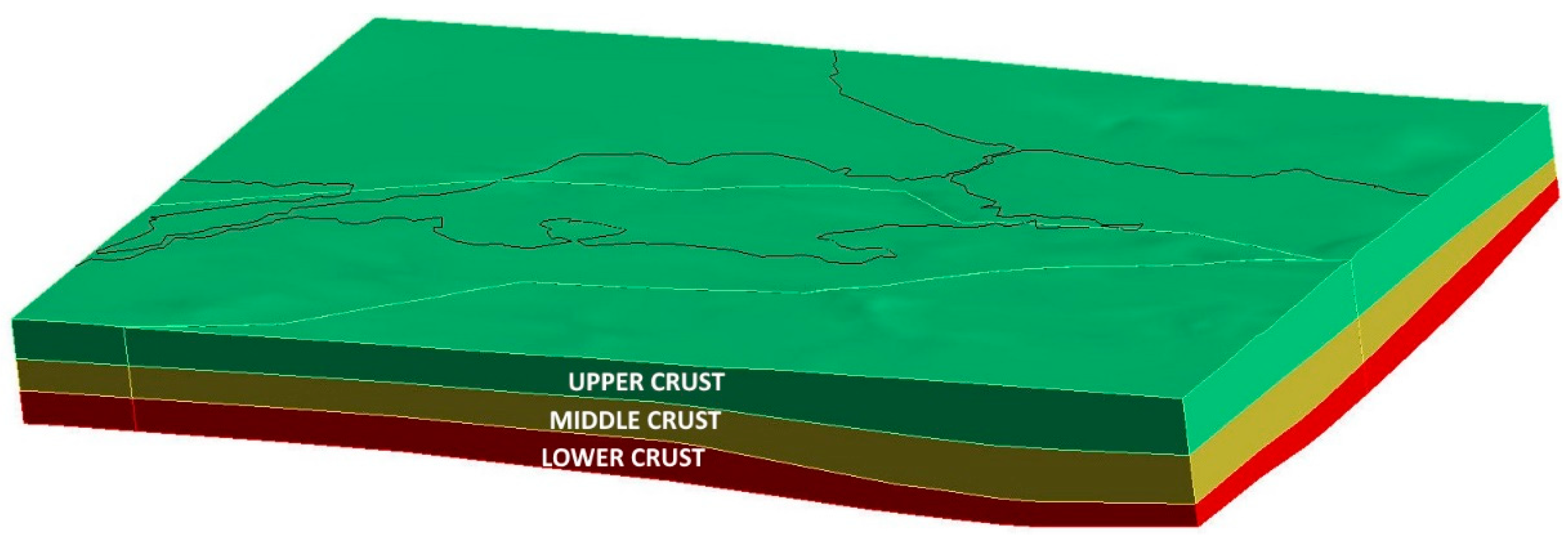
| Mean Depth (m) | Density (kg/m3) | (m/s) | (m/s) | E (GPa) | ν | |
|---|---|---|---|---|---|---|
| Upper Crust | ||||||
| Northern Part | 14,884 | 2783.202 | 6171.798 | 3595.387 | 89.452 | 0.243 |
| Middle Part | 2755.755 | 6130.727 | 3568.524 | 87.296 | 0.244 | |
| Southern Part | 2673.685 | 5951.101 | 3463.532 | 79.792 | 0.244 | |
| Middle Crust | ||||||
| Northern Part | 25,783 | 2870.239 | 6560.122 | 3789.549 | 103.013 | 0.250 |
| Middle Part | 2806.795 | 6374.402 | 3690.362 | 95.405 | 0.248 | |
| Southern Part | 2737.393 | 6239.372 | 3607.668 | 88.990 | 0.249 | |
| Lower Crust | ||||||
| Northern Part | 35,581 | 2991.605 | 7000.578 | 3899.408 | 116.004 | 0.275 |
| Middle Part | 2894.723 | 6703.498 | 3676.326 | 100.542 | 0.285 | |
| Southern Part | 2833.714 | 6626.517 | 3692.061 | 98.492 | 0.275 | |
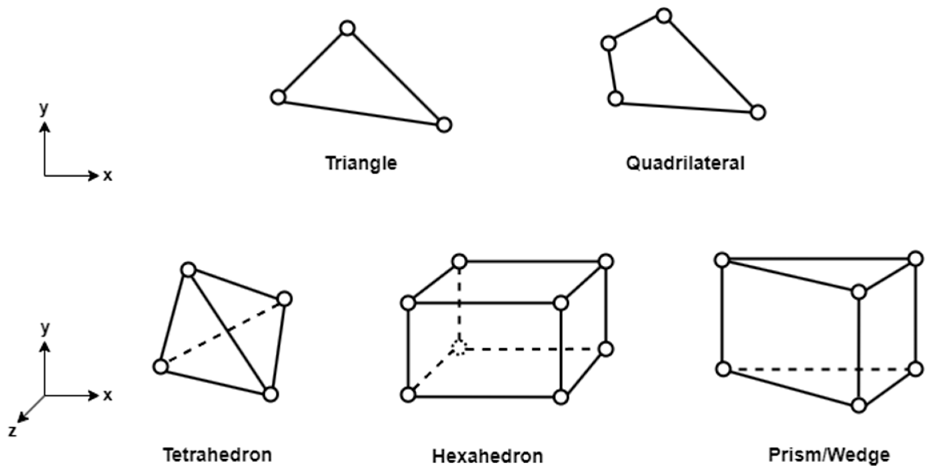
| Mesh Type | Face Mesh Type | Mapped Mesh Type | Number of Nodes | East RMSE (mm) | North RMSE (mm) |
|---|---|---|---|---|---|
| Tetrahedron | - | - | 487,279 | 1.53 | 1.09 |
| Sweep | Quad/Tri | - | 407,106 | 1.61 | 1.11 |
| Sweep | All Tri | - | 516,457 | 1.57 | 1.11 |
| Multizone | - | Hexa/Prism | 452,636 | 1.60 | 1.14 |
| Multizone | - | Hexa | 457,776 | 1.61 | 1.13 |
| Multizone | - | Prism | 614,995 | 1.65 | 1.12 |
Disclaimer/Publisher’s Note: The statements, opinions and data contained in all publications are solely those of the individual author(s) and contributor(s) and not of MDPI and/or the editor(s). MDPI and/or the editor(s) disclaim responsibility for any injury to people or property resulting from any ideas, methods, instructions or products referred to in the content. |
© 2023 by the authors. Licensee MDPI, Basel, Switzerland. This article is an open access article distributed under the terms and conditions of the Creative Commons Attribution (CC BY) license (https://creativecommons.org/licenses/by/4.0/).
Share and Cite
Karabulut, M.F.; Gülal, V.E. Accuracy Assessment of Mesh Types in Tectonic Modeling to Reveal Seismic Potential Using the Finite Element Method: A Case Study at the Main Marmara Fault. Appl. Sci. 2023, 13, 13297. https://doi.org/10.3390/app132413297
Karabulut MF, Gülal VE. Accuracy Assessment of Mesh Types in Tectonic Modeling to Reveal Seismic Potential Using the Finite Element Method: A Case Study at the Main Marmara Fault. Applied Sciences. 2023; 13(24):13297. https://doi.org/10.3390/app132413297
Chicago/Turabian StyleKarabulut, Mustafa Fahri, and Vahap Engin Gülal. 2023. "Accuracy Assessment of Mesh Types in Tectonic Modeling to Reveal Seismic Potential Using the Finite Element Method: A Case Study at the Main Marmara Fault" Applied Sciences 13, no. 24: 13297. https://doi.org/10.3390/app132413297
APA StyleKarabulut, M. F., & Gülal, V. E. (2023). Accuracy Assessment of Mesh Types in Tectonic Modeling to Reveal Seismic Potential Using the Finite Element Method: A Case Study at the Main Marmara Fault. Applied Sciences, 13(24), 13297. https://doi.org/10.3390/app132413297