

Stability Analysis of GNSS Stations Affected by Samos Earthquake

Abstract
1. Introduction
2. Materials and Methods
2.1. S-Transformation
2.2. Data and Process
3. Results and Discussion
4. Conclusions
Funding
Institutional Review Board Statement
Informed Consent Statement
Data Availability Statement
Acknowledgments
Conflicts of Interest
References
- Hekimoglu, S.; Erdogan, B.; Butterworth, S. Increasing the Efficacy of the Conventional Deformation Analysis Methods: Alternative Strategy. J. Surv. Eng. 2010, 136, 53–62. [Google Scholar] [CrossRef]
- Amiri-Simkooei, A.R.; Alaei-Tabatabaei, S.M.; Zangeneh-Nejad, F.; Voosoghi, B. Stability Analysis of Deformation-Monitoring Network Points Using Simultaneous Observation Adjustment of Two Epochs. J. Surv. Eng. 2017, 143, 04016020. [Google Scholar] [CrossRef]
- Aydin, C. Effects of Displaced Reference Points on Deformation Analysis. J. Surv. Eng. 2017, 143, 04017001. [Google Scholar] [CrossRef]
- Akpınar, B. Positioning Performance of GNSS-PPP and PPP-AR Methods for Determining the Vertical Displacements. Surv. Rev. 2021, 55, 68–74. [Google Scholar] [CrossRef]
- Even-Tzur, G. Extended S-Transformation as a Tool for Deformation Analysis. Surv. Rev. 2012, 44, 315–318. [Google Scholar] [CrossRef]
- Chen, Y.Q.; Chrzanowski, A.; Secord, J.M. A Strategy for the Analysis of the Stability of Reference Points in Deformation Surveys. CISM J. 1990, 44, 141–149. [Google Scholar] [CrossRef]
- Caspary, W.; Borutta, H. Robust estimation in deformation models. Surv. Rev. 1987, 29, 29–45. [Google Scholar] [CrossRef]
- Caspary, W. Concepts of Network and Deformation Analysis; University of New South Wales: Sydney, Australia, 2000. [Google Scholar]
- Wiśniewski, Z. Estimation of Parameters in a Split Functional Model of Geodetic Observations (M Split Estimation). J. Geod. 2009, 82, 105–120. [Google Scholar] [CrossRef]
- Wiśniewski, Z. M Split(q) Estimation: Estimation of Parameters in a Multi Split Functional Model of Geodetic Observations. J. Geod. 2010, 84, 355–372. [Google Scholar] [CrossRef]
- Zienkiewicz, M.H. Application of MSplit Estimation to Determine Control Points Displacements in Networks with Unstable Reference System. Surv. Rev. 2015, 47, 174–180. [Google Scholar] [CrossRef]
- Aydin, C. Power of Global Test in Deformation Analysis. J. Surv. Eng. 2012, 138, 51–56. [Google Scholar] [CrossRef]
- Jafari, M. Bayesian Approach in Stability Analysis of Monitoring Networks of Structures. Appl. Geomat. 2022, 14, 287–297. [Google Scholar] [CrossRef]
- Zienkiewicz, M.H. Identification of Unstable Reference Points and Estimation of Displacements Using Squared Msplit Estimation. Measurement 2022, 195, 111029. [Google Scholar] [CrossRef]
- Lim, M.C.; Setan, H.; Othman, R.; Chong, A.K. Deformation Detection for ISKANDARnet. Surv. Rev. 2012, 44, 198–207. [Google Scholar] [CrossRef]
- Guo, J.; Zhou, M.; Wang, C.; Mei, L. The Application of the Model of Coordinate S-Transformation for Stability Analysis of Datum Points in High-Precision GPS Deformation Monitoring Networks. J. Appl. Geod. 2012, 6, 143–148. [Google Scholar] [CrossRef]
- Even-Tzur, G. GPS Vector Configuration Design for Monitoring Deformation Networks. J. Geod. 2002, 76, 455–461. [Google Scholar] [CrossRef]
- Reilinger, R.E.; Ergintav, S.; Bürgmann, R.; McClusky, S.; Lenk, O.; Barka, A.; Gurkan, O.; Hearn, L.; Feigl, K.L.; Cakmak, R.; et al. Coseismic and Postseismic Fault Slip for the 17 August 1999, M = 7.5, Izmit, Turkey Earthquake. Science 2000, 289, 1519–1524. [Google Scholar] [CrossRef]
- Ergintav, S.; McClusky, S.; Hearn, E.; Reilinger, R.; Cakmak, R.; Herring, T.; Ozener, H.; Lenk, O.; Tari, E. Seven Years of Postseismic Deformation Following the 1999, M = 7.4 and M = 7.2, Izmit-Düzce, Turkey Earthquake Sequence. J. Geophys. Res. Solid Earth 2009, 114. [Google Scholar] [CrossRef]
- McClusky, S.; Balassanian, S.; Barka, A.; Demir, C.; Ergintav, S.; Georgiev, I.; Gurkan, O.; Hamburger, M.; Hurst, K.; Kahle, H.; et al. Global Positioning System Constraints on Plate Kinematics and Dynamics in the Eastern Mediterranean and Caucasus. J. Geophys. Res. 2000, 105, 5695–5719. [Google Scholar] [CrossRef]
- Chousianitis, K.; Konca, A.O. Rupture Process of the 2020 Mw7.0 Samos Earthquake and Its Effect on Surrounding Active Faults. Geophys. Res. Lett. 2021, 48, e2021GL094162. [Google Scholar] [CrossRef]
- Meng, J.; Sinoplu, O.; Zhou, Z.; Tokay, B.; Kusky, T.; Bozkurt, E.; Wang, L. Greece and Turkey Shaken by African Tectonic Retreat. Sci. Rep. 2021, 11, 6486. [Google Scholar] [CrossRef]
- Kiratzi, A.; Papazachos, C.; Özacar, A.; Pinar, A.; Kkallas, C.; Sopaci, E. Characteristics of the 2020 Samos Earthquake (Aegean Sea) Using Seismic Data. Bull. Earthq. Eng. 2021, 20, 7713–7735. [Google Scholar] [CrossRef]
- Taymaz, T.; Yolsal-Çevikbilen, S.; Irmak, T.S.; Vera, F.; Liu, C.; Eken, T.; Zhang, Z.; Erman, C.; Keleş, D. Kinematics of the 30 October 2020 Mw 7.0 Néon Karlovásion (Samos) Earthquake in the Eastern Aegean Sea: Implications on Source Characteristics and Dynamic Rupture Simulations. Tectonophysics 2022, 826, 229223. [Google Scholar] [CrossRef]
- Sakkas, V. Ground Deformation Modelling of the 2020 Mw6.9 Samos Earthquake (Greece) Based on InSAR and GNSS Data. Remote Sens. 2021, 13, 1665. [Google Scholar] [CrossRef]
- Foumelis, M.; Papazachos, C.; Papadimitriou, E.; Karakostas, V.; Ampatzidis, D.; Moschopoulos, G.; Kostoglou, A.; Ilieva, M.; Minos-Minopoulos, D.; Mouratidis, A.; et al. On Rapid Multidisciplinary Response Aspects for Samos 2020 M7.0 Earthquake. Acta Geophys. 2021, 69, 1025–1048. [Google Scholar] [CrossRef]
- Sboras, S.; Lazos, I.; Bitharis, S.; Pikridas, C.; Galanakis, D.; Fotiou, A.; Chatzipetros, A.; Pavlides, S. Source modelling and stress transfer scenarios of the 30 October 2020 Samos earthquake: Seismotectonic implications. Turk. J. Earth Sci. 2021, 30, 699–717. [Google Scholar] [CrossRef]
- Ganas, A.; Elias, P.; Briole, P.; Valkaniotis, S.; Escartin, J.; Tsironi, V.; Karasante, I.; Kosma, C. Co-Seismic and Post-Seismic Deformation, Field Observations and Fault Model of the 30 October 2020 Mw = 7.0 Samos Earthquake, Aegean Sea. Acta Geophys. 2021, 69, 999–1024. [Google Scholar] [CrossRef]
- Bulut, F.; Doğru, A.; Yaltirak, C.; Yalvac, S.; Elge, M. Anatomy of 30 October 2020, Samos (Sisam)-Kuşadası earthquake (MW 6.92) and its influence on Aegean earthquake hazard. Turk. J. Earth Sci. 2021, 30, 425–435. [Google Scholar] [CrossRef]
- Aktuğ, B.; Tiryakioğlu, İ.; Sözbilir, H.; Özener, H.; Özkaymak, Ç.; Yiğit, C.Ö.; Solak, H.İ.; Eyübagil, E.E.; Gelin, B.; Tatar, O.; et al. GPS Derived Finite Source Mechanism of the 30 October 2020 Samos Earthquake, Mw = 6.9, in the Aegean Extensional Region. Turk. J. Earth Sci. 2021, 30, 718–737. [Google Scholar] [CrossRef]
- Koch, K.-R. Parameter Estimation and Hypothesis Testing in Linear Models; Springer: Berlin/Heidelberg, Germany, 1999. [Google Scholar]
- Herring, T.A.; King, R.W.; Floyd, M.A.; McClusky, S.C. Introduction to Gamit/Globk, Release 10.7; Massachusetts Institute of Technology: Cambridge, MA, USA, 2018. [Google Scholar]
- Özarpacı, S.; Doğan, U.; Ergintav, S.; Çakır, Z.; Özdemir, A.; Floyd, M.; Reilinger, R. Present GPS Velocity Field along 1999 Izmit Rupture Zone: Evidence for Continuing Afterslip 20 Yr after the Earthquake. Geophys. J. Int. 2020, 224, 2016–2027. [Google Scholar] [CrossRef]
- Emre, Ö.; Duman, T.Y.; Özalp, S.; Elmacı, H.; Olgun, Ş.; ¸Şaroglu, F. Açıklamalı Türkiye Diri Fay Haritası. Ölçek 1:1.250.000; Maden Tetkik ve Arama Genel Müdürlüğü, Özel Yayın Serisi-30: Ankara, Turkey, 2013. [Google Scholar]
- Wessel, P.; Smith, W.H.F.; Scharroo, R.; Luis, J.; Wobbe, F. Generic Mapping Tools: Improved Version Released. Eos Trans. Am. Geophys. Union 2013, 94, 409–410. [Google Scholar] [CrossRef]


| Agency | ||||||||||
|---|---|---|---|---|---|---|---|---|---|---|
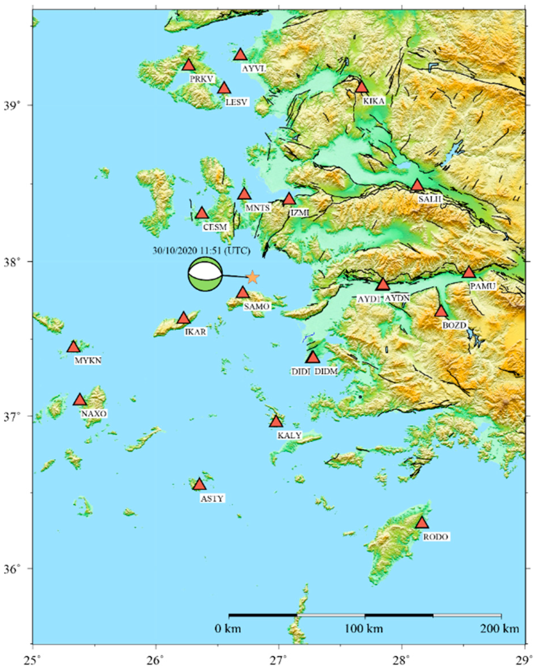
| AFAD | 26.794 | 37.902 | Mw6.9 | 17 km | 95 | 43 | −87 | 270 | 46 | −91 |
| USGS | 26.79 | 37.918 | Mw7.0 | 21 km | 93 | 61 | −91 | 276 | 29 | −88 |
| Station Name | (mm) | (mm) | (mm) | (mm) | (mm) | (mm) |
|---|---|---|---|---|---|---|
| ASTY | −2.43 | −6.82 | −8.84 | 13.04 | 7.09 | 9.71 |
| AYD1 | −1.91 | −3.05 | 3.14 | 12.23 | 7.30 | 9.65 |
| AYDN | −10.11 | −7.58 | −4.17 | 10.37 | 6.24 | 8.25 |
| AYVL | −1.03 | −2.37 | 6.06 | 8.61 | 4.86 | 7.09 |
| BOZD | −7.10 | −6.33 | −0.43 | 10.62 | 6.65 | 8.42 |
| CESM | −21.87 | −26.18 | 42.38 | 10.37 | 5.79 | 8.19 |
| DIDI | 0.69 | −2.63 | −6.40 | 10.70 | 6.25 | 8.18 |
| DIDM | −11.65 | −5.50 | −17.56 | 12.21 | 7.08 | 9.55 |
| IKAR | 23.70 | −4.45 | −22.85 | 11.77 | 6.67 | 9.52 |
| IZMI | −24.42 | 2.06 | 28.47 | 9.74 | 5.64 | 7.75 |
| KALY | 0.41 | 0.86 | −12.33 | 12.07 | 6.77 | 9.07 |
| KIKA | −2.83 | 0.03 | 4.24 | 9.36 | 5.84 | 7.88 |
| LESV | −6.94 | −4.53 | 6.66 | 12.38 | 6.78 | 9.99 |
| MNTS | −31.72 | −11.77 | 35.76 | 9.26 | 5.27 | 7.32 |
| MYKN | 0.25 | −2.00 | −2.07 | 10.42 | 5.35 | 7.76 |
| NAXO | −2.06 | −6.09 | −4.14 | 11.04 | 5.74 | 8.15 |
| PAMU | −15.35 | −9.92 | −10.72 | 11.88 | 7.59 | 9.86 |
| PRKV | −4.30 | −3.69 | 3.45 | 8.99 | 4.98 | 7.35 |
| RODO | 1.44 | −6.55 | −0.03 | 13.54 | 8.46 | 10.18 |
| SALH | −6.01 | −3.89 | −0.97 | 10.72 | 6.21 | 8.41 |
| SAMO | 290.44 | 75.35 | −236.92 | 13.79 | 8.03 | 11.05 |
| Station Name | Long. E° | Lat. N° | (mm) | (mm) | (mm) | (mm) | (mm) | (mm) |
|---|---|---|---|---|---|---|---|---|
| ASTY | 26.35332 | 36.54513 | −5.02 | −4.02 | 3.37 | 3.87 | −9.45 | 16.98 |
| AYD1 | 27.83788 | 37.84073 | −1.79 | 4.41 | 3.80 | 4.03 | −0.53 | 16.29 |
| AYDN | 27.84614 | 37.84700 | −1.97 | 4.37 | 3.09 | 3.24 | −12.42 | 13.95 |
| AYVL | 26.68618 | 39.31144 | −1.66 | 5.96 | 2.40 | 2.63 | 2.30 | 11.63 |
| BOZD | 28.31762 | 37.67294 | −2.20 | 5.33 | 3.21 | 3.33 | −7.58 | 14.37 |
| CESM | 26.37257 | 38.30381 | −13.73 | 52.76 | 3.25 | 3.41 | 1.77 | 14.41 |
| DIDI | 27.26866 | 37.37213 | −2.65 | −4.74 | 3.10 | 3.49 | −4.36 | 14.10 |
| DIDM | 27.27740 | 37.37335 | 0.45 | −6.16 | 3.74 | 3.93 | −20.89 | 16.15 |
| IKAR | 26.22423 | 37.62820 | −14.45 | −29.97 | 3.61 | 3.97 | 1.32 | 16.38 |
| IZMI | 27.08182 | 38.39481 | 12.93 | 35.33 | 2.81 | 3.09 | 1.38 | 13.01 |
| KALY | 26.97615 | 36.95580 | 0.58 | −10.34 | 3.73 | 4.51 | −6.81 | 15.73 |
| KIKA | 27.67220 | 39.10599 | 1.34 | 4.88 | 2.70 | 2.89 | 0.74 | 12.97 |
| LESV | 26.55379 | 39.10008 | −0.94 | 10.39 | 3.64 | 4.02 | −2.19 | 16.42 |
| MNTS | 26.71743 | 38.42658 | 3.75 | 49.06 | 2.60 | 2.87 | −4.12 | 12.33 |
| MYKN | 25.32907 | 37.44164 | −1.92 | −1.27 | 2.79 | 3.11 | −1.75 | 13.41 |
| NAXO | 25.38117 | 37.09819 | −4.62 | −0.60 | 3.03 | 3.42 | −6.06 | 14.15 |
| PAMU | 28.54335 | 37.92378 | −1.38 | 2.76 | 3.70 | 3.90 | −20.96 | 16.33 |
| PRKV | 26.26500 | 39.24570 | −1.40 | 6.16 | 2.46 | 2.68 | −2.07 | 12.11 |
| RODO | 28.16166 | 36.29260 | −6.45 | 1.05 | 3.95 | 4.57 | −1.49 | 17.94 |
| SALH | 28.12354 | 38.48309 | −0.60 | 3.70 | 3.06 | 3.37 | −6.19 | 14.27 |
| SAMO | 26.70533 | 37.79277 | −63.13 | −368.04 | 4.21 | 4.76 | 86.61 | 18.34 |
Disclaimer/Publisher’s Note: The statements, opinions and data contained in all publications are solely those of the individual author(s) and contributor(s) and not of MDPI and/or the editor(s). MDPI and/or the editor(s) disclaim responsibility for any injury to people or property resulting from any ideas, methods, instructions or products referred to in the content. |
© 2024 by the author. Licensee MDPI, Basel, Switzerland. This article is an open access article distributed under the terms and conditions of the Creative Commons Attribution (CC BY) license (https://creativecommons.org/licenses/by/4.0/).
Share and Cite
Özarpacı, S. Stability Analysis of GNSS Stations Affected by Samos Earthquake. Appl. Sci. 2024, 14, 2301. https://doi.org/10.3390/app14062301
Özarpacı S. Stability Analysis of GNSS Stations Affected by Samos Earthquake. Applied Sciences. 2024; 14(6):2301. https://doi.org/10.3390/app14062301
Chicago/Turabian StyleÖzarpacı, Seda. 2024. "Stability Analysis of GNSS Stations Affected by Samos Earthquake" Applied Sciences 14, no. 6: 2301. https://doi.org/10.3390/app14062301
APA StyleÖzarpacı, S. (2024). Stability Analysis of GNSS Stations Affected by Samos Earthquake. Applied Sciences, 14(6), 2301. https://doi.org/10.3390/app14062301