Multiple Watermarking Algorithms for Vector Geographic Data Based on Multiple Quantization Index Modulation

Featured Application

With the widespread application of digital watermarking technology, the number of users is rapidly increasing, creating new requirements. At the same time, in the era of big data, with sharing as the central theme, problems are arising related to multi-copyright protection and multilevel user tracking in the process of data production and the distribution and circulation of vector geographic data. This multiple digital watermarking algorithm can provide an effective solution to the above problems and was applied in software under test conditions.

Abstract

Multiple digital watermarking is an important and challenging task in geographic information science and data security. Vector geographic data are a basic data format for digital geographic data storage, and the security protection of these data involves copyright protection and tracking. As part of the solution, existing digital watermarking algorithms have made contributions to vector geographic data protection. However, when vector geographic data flow through multiple units, they need to be marked to ensure that the original data are not destroyed during data processing. Existing single or multiple data watermarking algorithms often fail in the presence of data processing because the new watermarks overlay the old ones. Consequently, a multiple digital watermarking algorithm based on multiple QIM (quantization index modulation) is proposed. First, based on traditional quantization index modulation (QIM), a multiple QIM is proposed. Unlike traditional QIM, in multiple QIM, the process of quantization is executed multiple times depending on the number of watermarks. Then, the vertices are quantized into different quantization intervals according to the multiple QIM. Finally, multiple watermarks are embedded into different quantization intervals to reduce the interference among multiple watermarks, and the original watermarks are not needed in the process of watermark detection. We then conducted experiments to test the multiple watermark method’s robustness and capacity, with an emphasis on datasets with a lower data volume. The experimental results show that the proposed algorithm achieves good performance in terms of its robustness against common issues, such as vertices addition, data simplification, data cropping, and feature deletion; this holds true for both normal and small amounts of data. Additionally, it has a high multiple watermark capacity.

1. Introduction

Vector geographic data represent the fundamental outcome of national infrastructure construction and play a pivotal role in driving social and economic development. Nowadays, computer technology and networking are highly developed. As a digital media product, vector geographic data are becoming ever more convenient in terms of acquisition, replication, dissemination, and application. The question of how to effectively protect and track the copyright of vector geographic data has become an important technical problem to be solved in the field of information security. The application prospects of digital watermarking technology in securing vector geographic data are highly significant. Numerous scholars have extensively investigated digital watermarking technology for vector geographic data, yielding a plethora of valuable research findings [1,2,3,4,5,6,7,8,9,10,11]. The current research on digital watermarking technology for vector geographic data primarily focuses on robust and fragile watermarking techniques, which are predominantly employed to address issues related to data copyright protection, single-user usage tracking, and content authentication.

With the continuous advancement of data management and distribution technology, the transmission of vector geographic data has become increasingly convenient. During the transmission process, vector geographic data may undergo multiple transformations and be accessed by various entities. The security protection of vector geographic data based on digital watermarking technology entails novel challenges. For example, different distributors are allowed to embed multiple different watermarks in the same cover data, either in heterogeneous time and space or not. The original watermarks can still be effectively detected when the cover data containing the watermarks are embedded in another watermark. The question therefore remains as to how to effectively implement the whole process of multi-user tracking; this issue cannot be solved using a single watermarking algorithm. Multiple watermarking technology represents a good method for solving the above problems. The term “multiple watermarking technology” refers to the embedding of multiple distinct watermarks within the same cover data. This technology serves the purpose of safeguarding copyright and facilitating the tracking of “multi-user” usage during data distribution and transmission processes. However, the existing multiple watermarking technology places more focus on the algorithms for digital images that have the following three main types. The first is the combination of different types of watermarking, such as robust watermarking, fragile watermarking, zero watermarking, or reversible watermarking [12,13]. The second is embedding watermarks in different locations that constitute spatial and frequency domains [14,15,16,17,18,19,20], as well as different blocks of the spatial domain [21,22,23,24]. The last involves consolidating the multiple watermarks into a single watermark, which is subsequently embedded into the cover data using a normal single watermarking algorithm [25,26,27].

Vector geographic data are different from digital images because they are organized by coordinate vertices. Therefore, the above methods cannot be directly applied to the multiple watermarking algorithm for vector geographic data. For vector geographic data, adding, deleting, and randomly changing coordinate vertices are common operations; meanwhile, embedding sufficient watermarks is a challenge for vector geographic data containing fewer vertices. However, the concepts used to solve the problem for digital images can be used as a reference. To the best of our knowledge, limited research has been conducted on vector geographic data, and the algorithms that are used to embed multiple watermarks learn from those intended for digital images. For instance, in [28], robust watermarks and fragile watermarks were embedded into the feature and non-feature vertices of cover data. In [29], combined with the Arnold algorithm, a zero watermark was constructed according to feature vertices’ information, and a non-destructive fragile watermark was used to authenticate the data content via spatial sorting and zero-bit dynamic expansion. In [30], two types of watermarks, namely, a zero watermark and a reversible watermark, were employed. The density center vertices were selected to embed the zero watermark, while the feature vertices located within a relative distance to the density center were utilized to embed the reversible watermark. The above three algorithms all combine general watermarking and zero watermarking or reversible watermarking to embed two watermarks, and the watermark capacity is limited. In [31,32], two watermarks were embedded in the spatial domain and the frequency domain. In [33], four kinds of multiple watermarking algorithms were designed. One embedded two watermarks in the DFT (Discrete Fourier Transform) and DCT (Discrete Cosine Transformation) domains, while another embedded three watermarks in the low-, intermediate-, and high-frequency domains. The number of embedding watermarks in the above studies is limited by the type of watermarking algorithm. These algorithms embed two watermarks into different frequency domains. The number of frequency domains is limited, which limits the number of embedded watermarks. Consequently, as frequency domain watermarking algorithms, they have weaknesses in terms of resisting addition and deletion attacks. In [34,35,36], the cover data were divided into many blocks or vertices sets, in which multiple different watermarks were embedded. Enough coordinate vertices need to be provided so that multiple watermarks are not overwritten. In [37], dual watermarks were formed by combining a copyright watermark, which utilized copyright information, with another watermark composed of features selected via fuzzy c-means clustering from the vector geographic data. Subsequently, these newly composed watermarks were embedded into the cover data using a single watermarking algorithm. The watermarks, designed based on QR codes (Quick Response Codes), were embedded into the polar coordinates of the vector geographic vertices in [38]. Prior to embedding all of the watermarks, the locations for embedding should be reserved according to the number of watermarks intended for insertion.

In order to ensure the preservation of all watermarks in the watermarked data, even after common adding and deleting attacks, and when embedding sufficient watermarks in vector geographic data containing fewer coordinate vertices, we proposed a novel multiple watermarking algorithm based on multiple QIM for vector geographic data.

The subsequent sections of this paper are structured as follows: Section 2 presents the proposed method, multiple quantization index modulation. Subsequently, Section 3 provides a detailed introduction to the multiple watermarking algorithm for vector geographic data. The experimental results and performance evaluations are presented in Section 4. Finally, concluding remarks and the study’s identified limitations are discussed in Section 5.

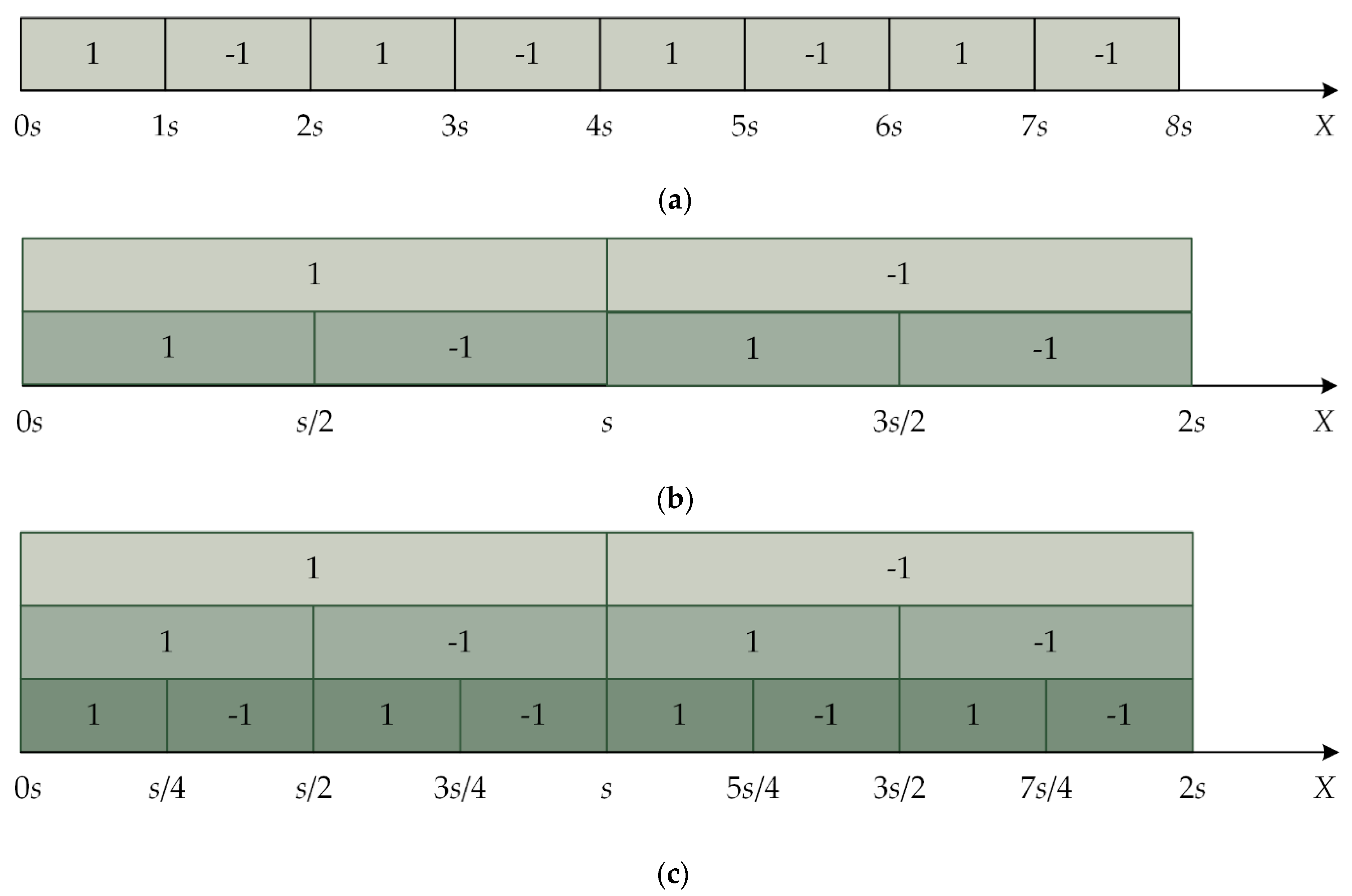
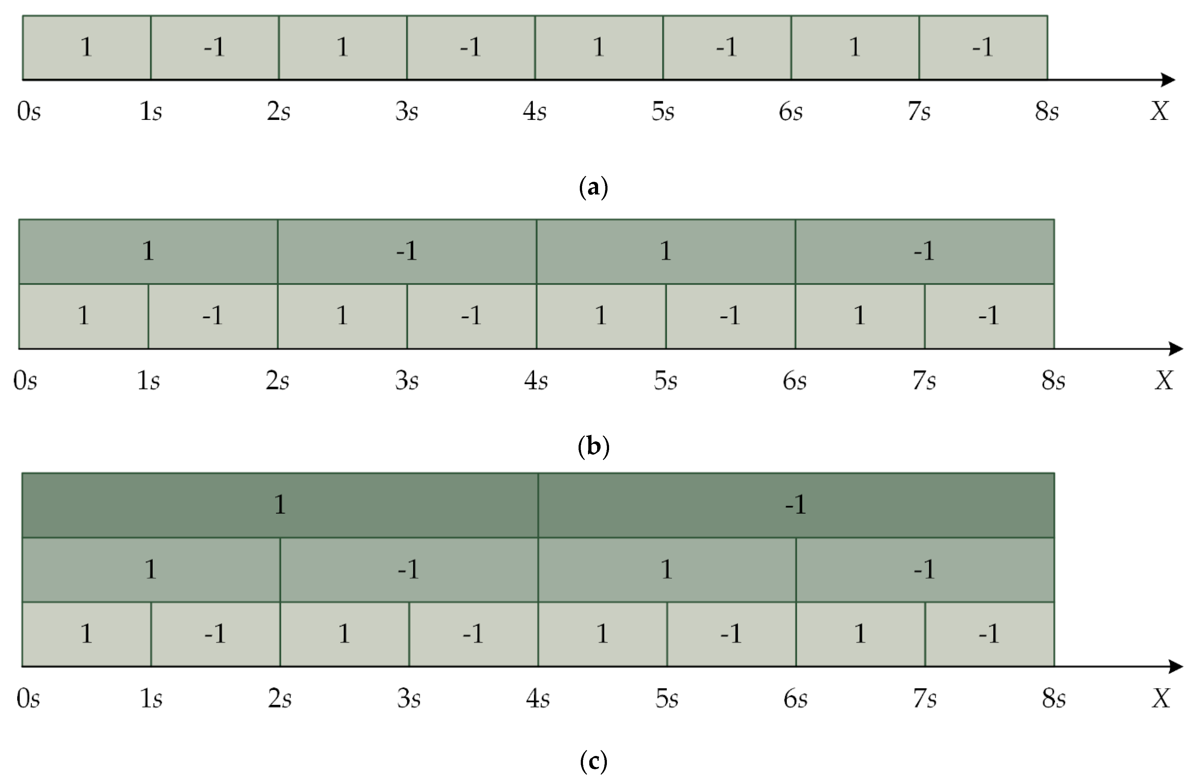
2. QIM and Multiple QIM

Watermark algorithms generally involve three steps: watermark generation, watermark embedding, and watermark detection. The robustness of the algorithm is usually used to evaluate the quality of watermark algorithms. Robustness pertains to the capacity of the embedded watermarks to retain their attributes in the cover data following data processing. In order to ensure the robustness of a watermarking algorithm, as discussed in Section 1, scholars often focus on designing special mechanisms during the embedding stage, while the proposed algorithm employs a novel embedding approach during this stage.

Quantization index modulation (QIM), achieved by modulating the host data with the embedded information, has become a popular watermark-embedding algorithm because it is a method that rejects host interference and has provably good performance in terms of rate distortion robustness [39]. The vector geographic data comprise the fundamental units of points, polylines, and polygons, represented by coordinate vertices. These vertices are utilized to embed watermark bits for implementing the watermarking algorithm. The QIM technique modulates an index with the watermarks and subsequently quantizes the coordinate vertices of the vector geographic data into different quantization intervals based on the associated quantizer. The watermarks are divided into meaningful and meaningless watermarks. In the proposed algorithm, the meaningless watermarks, pseudorandom binary sequences comprising 1 and −1, which distribute randomly, were used to embed more watermarks. The random 1 or −1 is called the watermark bit. The vertices coordinates of the cover vector geographic data are divided into several intervals according to the change in the watermark bits, which is referred to as QIM. Figure 1 shows the rule of QIM. The $X$ values of the vertices are quantized into −1 and 1 intervals, where $s$ represents the quantization step size.

The vertices coordinates of the cover data are denoted as $vc$, in accordance with the watermark embedding rule:

$$\left\{\begin{array}{c}vc=vc+s if (((vc\%(2\ast s))<s)\&\&(wb==1))\\ vc=vc-s if (((vc\%(2\ast s))\ge s)\&\&(wb==-1))\end{array}\right.,$$

(1)

where wb is the embedding watermark bit. Similarly, the watermark extraction rule is followed:

$$\left\{\begin{array}{c}wb==-1 if (vc\%(2\ast s))<s)\\ wb==1 if (vc\%(2\ast s))\ge s)\end{array}\right..$$

(2)

The above represents the QIM technique for a single watermark algorithm. By adhering to the rules of the single quantization index, it becomes possible to repeatedly embed one watermark within the cover data, thereby enhancing its robustness. Considering the characteristics of the single quantization index, the intervals can be quantized many times based on the original quantization index rule to embed multiple watermarks. The multiple quantization index includes the up–down and down–up quantization indexes, according to different quantization orders.

In the up–down quantization, half of the quantization step size is used as the next one. In Figure 2a, $0~2s$ is the interval to be quantized, and the first step size is $s$. The second quantization step size is $s/2$, as shown in Figure 2b. The third quantization step size is $s/4$, as shown in Figure 2c. In this way, this process goes on until multiple watermarks are embedded. The rules of watermark extraction are shown in

Table 1. Rules of watermark extraction corresponding to the up–down MQIM.

Watermarks	Intervals of Cover Coordinate Vertices	Watermark Bits
First watermark	$vc\%(2\ast s)<s$	−1
	$vc\%(2\ast s)\ge s$	1
Second watermark	$vc\%s<s/2$	−1
	$vc\%s\ge s/2$	1
Third watermark	$vc\%(s/2)<s/4$	−1
	$vc\%(s/2)\ge s/4$	1

, corresponding to the up–down multiple quantization mechanism.

The next quantization step size is twice the original quantization step size in the down–up quantization mechanism, as shown in Figure 3. In Figure 3a, $0~8s$ is the interval to be quantized, and the first step size is $s$. The second quantization step size is $2s$, as shown in Figure 3b. The third quantization step size is $4s$, as shown in Figure 3c. The process continues in this way until multiple watermarks are embedded. The rules of watermark extraction are shown in

Table 2. Rules of watermark extraction corresponding to the down–up MQIM.

Watermarks	Intervals of Cover Coordinate Vertices	Watermark Bits
First watermark	$vc\%(2\ast s)<s$	−1
	$vc\%(2\ast s)\ge s$	1
Second watermark	$vc\%(4\ast s)<2\ast s$	−1
	$vc\%(4\ast s)\ge 2\ast s$	1
Third watermark	$vc\%(8\ast s)<4\ast s$	−1
	$vc\%(8\ast s)\ge 4\ast s$	1

.

Figure 2 and Figure 3 show that more than one watermark bit can be embedded in a single coordinate based on the multi-quantization mechanism, and, at the same time, different watermark information bits will not interfere with each other. In the up–down quantization mechanism, the quantization step size becomes smaller with an increase in quantization time, whereas, in the down–up quantization mechanism, the quantization step size becomes bigger. Considering that the number of watermarks to be embedded is unknown, the up–down quantization mechanism is better for controlling embedding errors. This mechanism is adopted in Section 3.

3. Proposed Multiple Watermarking Algorithm

With the aim of incorporating multiple watermarks and ensuring resilience against common attacks, a novel algorithm for multiple watermarking is proposed. Figure 4 shows the proposed embedding procedure based on MQIM. First, the coordinate vertices of the cover vector geographic data are quantized into non-overlapping quantization intervals using up–down MQIM. Each embedding watermark is embedded into the corresponding quantization interval to avoid them disturbing each other. Then, during the processing of watermark detection, all watermarks are extracted, and correlation detection is undertaken to detect multiple watermarks.

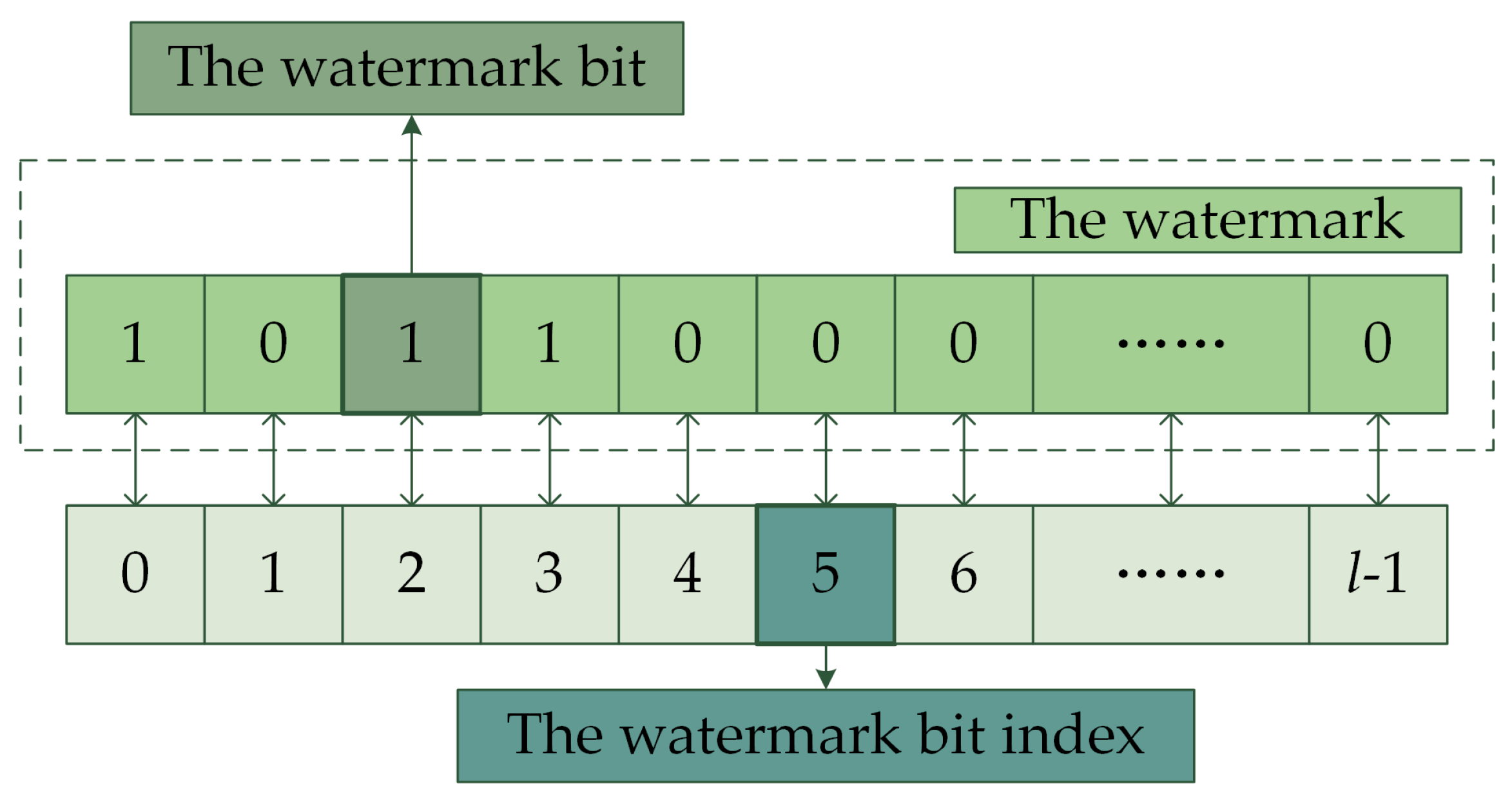
3.1. Watermark Generation

Meaningless watermarks are adopted in the proposed algorithm. The length of the meaningless watermark is shorter than that of the meaningful watermark, and there is a small amount of vector geographic data. To embed more watermarks, a pseudo-random binary sequence, one kind of meaningless watermark, is adopted in the paper.

A pseudo-random binary sequence generator is used to generate different meaningless watermark information. Let the watermark be $W_m$. It is presented in the expression below:

$$W_m=\left\{w_m\left[i\right], 0\le i<l\right\}$$

(3)

where the watermark bit is denoted as $w_m\left[i\right]$, $w_m\left[i\right]\in \left\{0,1\right\}$, the number of the watermark is denoted as $m$, the watermark bit index is denoted as $i$, and the length of the watermark is denoted as $l$. The statistical characteristics of $w_m\left[i\right]$ are given by $P\left(w_m\left[i\right]=0\right)=1/2$ and $P\left(w_m\left[i\right]=1\right)=1/2$, indicating that the probability of being equal to either 0 or 1 is equally likely for each bit in the watermark. Considering that the volume of some vector geographic data is small, $l$ is 200 in the following sections.

In the subsequent section, the terms watermark, watermark bit, and watermark bit index are frequently referenced. The interrelationships between these concepts are illustrated in Figure 5.

3.2. Watermark Embedding

Spatial domain watermarking is when the watermarks are directly embedded in the coordinates of the vector graphic data. Generally, to increase robustness against common attacks, especially data cropping and the deletion of vertices, the same watermarks are usually repeatedly embedded into vector geographic data. That is, the same watermark bit may be embedded into different coordinates, generating robustness against vertex deletion attacks. Generally, common attacks include data addition and deletion. Data addition attacks involve randomly adding vertices to the watermarked data, while data deletion attacks remove vertices from the cover data. There are four types of data deletion attacks: deleting vertices (depicted in Figure 6), deleting features (illustrated in Figure 7), data cropping (illustrated in Figure 8), and data compression attacks. Deleting vertices involves randomly removing vertices from the watermarked data; deleting features means randomly deleting points, polylines, or polygons from the watermarked data; data cropping attacks involve selectively cropping regions of the watermarked data; and data compression attacks involve compressing the vector map with the watermark the Douglas–Peucker algorithm [40]. For vector geographic data organized as points, deleting vertices is the same as deleting features. The attack intensity corresponds to the number of vertices being processed divided by the number of original data.

The proposed algorithm is based on the fundamental concept that watermark bits are repeatedly embedded in different coordinates using a “one-to-many” mapping between watermark bit indexes and coordinates. In other words, each watermark bit is embedded multiple times in various coordinates. Consequently, a single watermark bit index may correspond to several coordinates, enhancing robustness against vertex deletion attacks. Figure 9 illustrates the “one-to-many” relationship, while Equation (4) presents the embedding model.

In Figure 9, there are four watermarks, watermarks 1, 2, 3, and 4, and the cover data that are composed of coordinate vertices. The watermark bits corresponding to the same index are embedded into a single coordinate:

$$VC\oplus W=\left\{x_j\oplus w_i\left[f\left(x_j,y_j\right)\right]\right\},$$

(4)

where $VC$ refers to the cover data, $W$ is a watermark, $\left(x_j,y_j\right)$ are the coordinates of the $i$th vertices, and $f(·)$ is the mapping relationship between the coordinate vertices and the watermark bit indexes. Moreover, in Equation (4), $0\le f(·)<l$, where $l$ is the length of the watermarks. $\oplus$ is the method of watermark embedding, that is, the proposed multiple watermarking method using MQIM. The watermarks are embedded in the $X$ coordinates. The whole flow for embedding the four watermarks is shown in Figure 10, and the specific embedding steps are followed.

(1)

Let the first quantization step size be $s$, and the number of embedding watermarks be $m$. The watermark index is initialized as $0$, i.e., $i=0$.

(2)

The index of the watermark bit is $i=f\left(x_j,y_j\right)$ for the vertices $\left(x_j,y_j\right)$. The index of the embedding watermark bit $wb$ is $w_k\left[i\right]$.

(3)

According to step $s$ and the watermark index $k$, the rules of the watermark bit $wb$ embedding into the vertices are given in Equation (5):

$$\left\{\begin{array}{c}{x^{\prime }}_j=x_j+\frac{s}{2^k}if \left(\left(\left(x_j\%\frac{s}{2^{k-1}}\right)\right)<\frac{s}{2^k}\right)|\left(wb==1\right)\\ {x^{\prime }}_j=x_j-\frac{s}{2^k}if \left(\left(\left(x_j\%\frac{s}{2^{k-1}}\right)\right)\ge \frac{s}{2^k}\right)|\left(wb==-1\right)\end{array}\right.,$$

(5)

where $\left({x^{\prime }}_j,{y^{\prime }}_j\right)$ is the coordinate of the $j$th vertex embedded in the watermark corresponding to $\left(x_j,y_j\right)$.

(4)

Steps (2) and (3) are not repeated until the watermark, $W_k$, is embedded in the cover data.

(5)

If $k=m$, the embedding of the watermark is finished; let $k=k+1$ and skip to Step (2).

An erroneous change in coordinates can occur, whereby several watermark bits are embedded in the same vertices coordinate in the process of watermark embedding; this issue needs to be addressed. Let the $X$ value of the vertex’s coordinate be ${x^{\prime }}_j$ after embedding $M$ watermark bits. The upper limited of absolute error for coordinate variation is shown in Equation (6):

$${\delta }_j={x^{\prime }}_j-x_j\le {\displaystyle \sum _{k=0}^M\frac{s}{2^k}},$$

(6)

where ${\delta }_j$ is the upper limit of the absolute error for the $j$th vertex’s coordinate. When $M\to \infty$, $\underset{M\to \infty }{\lim }{\displaystyle \sum _{k=0}^M\frac{s}{2^k}}=2s$. Therefore, when the quantization step is $s$, the upper limit of the error variation of a single coordinate caused by multiple watermark embedding is $2s$. In other words, when multiple watermarks are embedded via up–down multiple quantization, the change in the coordinate error is controllable. The initial quantization step can be appropriately selected based on the accuracy requirements of the data in order to control the range of coordinate variation caused by multiple watermarks being effectively embedded.

3.3. Watermark Extraction and Detection

The extraction of watermark bits is achieved using the inverse of the process used for embedding watermarks. The procedure for extracting and detecting watermark bits can be summarized as follows:

(1)

Let the initialized quantization step size be $s$, and the value in the embedding process $s$. Let the index of the extracting watermark be $k^{\prime }$, and $k^{\prime }=0$.

(2)

Initialize the watermark bits’ storage array, $W^{\prime }=\left\{w^{\prime }\left[i\right], 0\le i<N\right\}$, and let $w^{\prime }\left[i\right]=0$.

(3)

For the vertices coordinates $\left(x_j,y_j\right)$, the index of the watermark bit is calculated: $index=f\left(x_j,y_j\right)$.

(4)

The potential watermark bits in the vertices, $w{b}^{\prime }$, are extracted according to the following Equation (7):

$$\left\{\begin{array}{c}w{b}^{\prime }=-1 if(d\%(\frac{s}{2^{k-1}}))<\frac{s}{2^k}\\ w{b}^{\prime }=1 if(d\%(\frac{s}{2^{k-1}}))\ge \frac{s}{2^k}\end{array}\right..$$

(7)

(5)

Save the extracted watermark bits in $W^{\prime }$, and $w^{\prime }\left[f\left(x_j,y_j\right)\right]=w^{\prime }\left[f\left(x_j,y_j\right)\right]+wb$.

(6)

For all coordinate vertices, steps (2) to (5) are repeated to extract all watermark sets, $W^{\prime }$.

(7)

The relationship between the watermark bits and coordinate vertices is “many to one”, therefore, let $w^{\prime }\left[i\right]=1$ if $w^{\prime }\left[i\right]>0$. Let $w^{\prime }\left[i\right]=-1$ if $w^{\prime }\left[i\right]<0$, and $w^{\prime }\left[i\right]=1$ or $w^{\prime }\left[i\right]=-1$ randomly, if $w^{\prime }\left[i\right]=0$.

(8)

The original watermarks are correlated with the extracted watermarks in order to assess whether they are the original watermarks or not. These watermarks are stored if the extracted watermark is the embedded one; otherwise, let $k^{\prime }=k^{\prime }+1$ and skip to Step (2). The detection is not complete until $k^{\prime }=k$.

4. Experiments and Results

The proposed multiple watermarking algorithm was implemented to validate its performance, utilizing ShapeFile format data for the experiments. Specifically, an in-depth analysis was conducted to assess the robustness of the algorithm against random noise attacks and its capacity to handle multiple watermarks.

4.1. Algorithm Robustness

Robustness refers to the ability of multiple watermarking techniques to detect watermarks in the cover data, even after being subjected to various attacks. For vector geographic data, the most common attacks are randomly deleting vertices, cropping, compression, or randomly adding vertices. The proposed multiple watermarking algorithm was evaluated for its robustness via experiments conducted on diverse digital vector geographic maps in the ShapeFile format. Figure 11 shows three example maps of experimental data, which (a) are organized as points, (b) are organized as polylines and (c) are organized as polygons.

The same experimental procedures were repeated for different vector geographic datasets, numbered from 1 to 30. Nos. 1 to 10 are organized as points, 11 to 20 are organized as polylines, and 21 to 30 are organized as polygons, sorted in ascending order based on the number of coordinate vertices in the cover data. A multiple watermarking algorithm with good robustness against data addition and deletion attacks is presented in [35]; therefore, it is chosen for the comparative experiments. In [35], the vector geographic data are divided into logic domains according to the number of watermarks, and then the watermarks are embedded into the cover data. This algorithm exhibits good performance in terms of robustness against the deletion of vertices and cropping attacks.

The specific steps of the experiment were followed meticulously. Four watermarks were randomly generated. The experimental cover data successively embed Watermark 1, Watermark 2, Watermark 3, and Watermark 4 using both the proposed algorithm in Section 3 and the algorithm proposed in [35]. Then, the random deletion of vertices, cropping, compression, and the random addition of vertices are carried out. Finally, all watermarks are detected in the cover data being attacked. The detection process does not involve the original vector map or the original watermark, i.e., the blind watermarking algorithm. We conducted 30 experiments to repeat the above experimental procedure. The corresponding experimental results for the experimental maps are presented in

Table 3. Experimental results for maps 1–10 for the random addition and deletion of vertices.

Attacks	Attacks Intensity	Detected Results
		Watermark 1		Watermark 2		Watermark 3		Watermark 4
		Proposed Algorithm	Reference [35] Algorithm	Proposed Algorithm	Reference [35] Algorithm	Proposed Algorithm	Reference [35] Algorithm	Proposed Algorithm	Reference [35] Algorithm
No attacks	0%	√ (No. 1–10)	√ (No. 1–10)	√ (No. 1–10)	√ (No. 1–10)	√ (No. 1–10)	√ (No. 1–10)	√ (No. 1–10)	√ (No. 1–10)
Deleting features	30%	√ (No. 1–10)	√ (No. 1–10)	√ (No. 1–10)	√ (No. 1–10)	√ (No. 1–10)	√ (No. 1–10)	√ (No. 1–10)	√ (No. 1–10)
	50%	√ (No. 1–10)	√ (No. 1–10)	√ (No. 1–10)	√ (No. 1–10)	√ (No. 1–10)	√ (No. 1–10)	√ (No. 1–10)	√ (No. 1–10)
	70%	√ (No. 1–10)	√ (No. 1–10)	√ (No. 1–10)	√ (No. 1–10)	√ (No. 1–10)	√ (No. 1–10)	√ (No. 1–10)	√ (No. 1–10)
	90%	√ (No. 1–10)	√ (No. 1–10)	√ (No. 1–10)	√ (No. 1–10)	√ (No. 1–10)	√ (No.9–10)	√ (No. 1–10)	√ (No. 10)
Cropping	10–20%	√ (No. 1–10)	√ (No. 1–10)	√ (No. 1–10)	√ (No. 1–10)	√ (No. 1–10)	√ (No. 1–10)	√ (No. 1–10)	√ (No. 1–10)
	40–50%	√ (No. 1–10)	√ (No. 1–10)	√ (No. 1–10)	√ (No. 1–10)	√ (No. 1–10)	√ (No. 1–10)	√ (No. 1–10)	√ (No. 1–10)
	70–80%	√ (No. 1–10)	√ (No. 1–10)	√ (No. 1–10)	√ (No. 1–10)	√ (No. 1–10)	√ (No. 1–10)	√ (No. 1–10)	√ (No. 1–10)
	80–90%	√ (No. 1–10)	√ (No. 1–10)	√ (No. 1–10)	√ (No. 1–10)	√ (No. 1–10)	√ (No.9–10)	√ (No. 1–10)	√ (No. 10)
Adding vertices	30%	√ (No. 1–10)	√ (No. 1–10)	√ (No. 1–10)	√ (No. 1–10)	√ (No. 1–10)	√ (No. 1–10)	√ (No. 1–10)	√ (No. 1–10)
	50%	√ (No. 1–10)	√ (No. 1–10)	√ (No. 1–10)	√ (No. 1–10)	√ (No. 1–10)	√ (No. 1–10)	√ (No. 1–10)	√ (No. 1–10)
	70%	√ (No. 1–10)	√ (No. 1–10)	√ (No. 1–10)	√ (No. 1–10)	√ (No. 1–10)	√ (No. 1–10)	√ (No. 1–10)	√ (No. 1–10)
	90%	√ (No. 1–10)	√ (No. 1–10)	√ (No. 1–10)	√ (No. 1–10)	√ (No. 1–10)	√ (No. 1–10)	√ (No. 1–10)	√ (No. 1–10)

,

Table 4. Experimental results for maps 11–20 for the random addition and deletion of vertices.

Attacks	Attacks Intensity	Detected Results
		Watermark 1		Watermark 2		Watermark 3		Watermark 4
		Proposed Algorithm	Reference [35] Algorithm	Proposed Algorithm	Reference [35] Algorithm	Proposed Algorithm	Reference [35] Algorithm	Proposed Algorithm	Reference [35] Algorithm
No attacks	0%	√ (No. 11–20)	√ (No. 11–20)	√ (No. 11–20)	√ (No. 11–20)	√ (No. 11–20)	√ (No. 11–20)	√ (No. 11–20)	√ (No. 11–20)
Deleting vertices	30%	√ (No. 11–20)	√ (No. 11–20)	√ (No. 11–20)	√ (No. 11–20)	√ (No. 11–20)	√ (No. 11–20)	√ (No. 11–20)	√ (No. 11–20)
	50%	√ (No. 11–20)	√ (No. 11–20)	√ (No. 11–20)	√ (No. 11–20)	√ (No. 11–20)	√ (No. 11–20)	√ (No. 11–20)	√ (No. 11–20)
	70%	√ (No. 11–20)	√ (No. 11–20)	√ (No. 11–20)	√ (No. 11–20)	√ (No. 11–20)	√ (No. 11–20)	√ (No. 11–20)	√ (No. 11–20)
	90%	√ (No. 11–20)	√ (No. 11–20)	√ (No. 11–20)	√ (No. 11–20)	√ (No. 11–20)	√ (No. 11–20)	√ (No. 11–20)	√ (No. 18–20)
Deleting features	30%	√ (No. 11–20)	√ (No. 11–20)	√ (No. 11–20)	√ (No. 11–20)	√ (No. 11–20)	√ (No. 11–20)	√ (No. 11–20)	√ (No. 11–20)
	50%	√ (No. 11–20)	√ (No. 11–20)	√ (No. 11–20)	√ (No. 11–20)	√ (No. 11–20)	√ (No. 11–20)	√ (No. 11–20)	√ (No. 11–20)
	70%	√ (No. 11–20)	√ (No. 11–20)	√ (No. 11–20)	√ (No. 11–20)	√ (No. 11–20)	√ (No. 11–20)	√ (No. 11–20)	√ (No. 11–20)
	90%	√ (No. 11–20)	√ (No. 11–20)	√ (No. 11–20)	√ (No. 11–20)	√ (No. 11–20)	√ (No. 11–20)	√ (No. 11–20)	√ (No. 18–20)
Cropping	10–20%	√ (No. 11–20)	√ (No. 11–20)	√ (No. 11–20)	√ (No. 11–20)	√ (No. 11–20)	√ (No. 11–20)	√ (No. 11–20)	√ (No. 11–20)
	40–50%	√ (No. 11–20)	√ (No. 11–20)	√ (No. 11–20)	√ (No. 11–20)	√ (No. 11–20)	√ (No. 11–20)	√ (No. 11–20)	√ (No. 11–20)
	70–80%	√ (No. 11–20)	√ (No. 11–20)	√ (No. 11–20)	√ (No. 11–20)	√ (No. 11–20)	√ (No. 11–20)	√ (No. 11–20)	√ (No. 11–20)
	80–90%	√ (No. 11–20)	√ (No. 11–20)	√ (No. 11–20)	√ (No. 11–20)	√ (No. 11–20)	√ (No. 11–20)	√ (No. 11–20)	√ (No. 19–20)
Compression	10–20%	√ (No. 11–20)	√ (No. 11–20)	√ (No. 11–20)	√ (No. 11–20)	√ (No. 11–20)	√ (No. 11–20)	√ (No. 11–20)	√ (No. 11–20)
	20–30%	√ (No. 11–20)	√ (No. 11–20)	√ (No. 11–20)	√ (No. 11–20)	√ (No. 11–20)	√ (No. 11–20)	√ (No. 11–20)	√ (No. 11–20)
	30–40%	√ (No. 11–20)	√ (No. 11–20)	√ (No. 11–20)	√ (No. 11–20)	√ (No. 11–20)	√ (No. 11–20)	√ (No. 11–20)	√ (No. 11–20)
	40–50%	√ (No. 11–20)	√ (No. 11–20)	√ (No. 11–20)	√ (No. 11–20)	√ (No. 11–20)	√ (No. 16–20)	√ (No. 11–20)	√ (No. 17–20)
Adding vertices	30%	√ (No. 11–20)	√ (No. 11–20)	√ (No. 11–20)	√ (No. 11–20)	√ (No. 11–20)	√ (No. 11–20)	√ (No. 11–20)	√ (No. 11–20)
	50%	√ (No. 11–20)	√ (No. 11–20)	√ (No. 11–20)	√ (No. 11–20)	√ (No. 11–20)	√ (No. 11–20)	√ (No. 11–20)	√ (No. 11–20)
	70%	√ (No. 11–20)	√ (No. 11–20)	√ (No. 11–20)	√ (No. 11–20)	√ (No. 11–20)	√ (No. 11–20)	√ (No. 11–20)	√ (No. 11–20)
	90%	√ (No. 11–20)	√ (No. 11–20)	√ (No. 11–20)	√ (No. 11–20)	√ (No. 11–20)	√ (No. 11–20)	√ (No. 11–20)	√ (No. 11–20)

and

Table 5. Experimental results for maps 21–30 for the random addition and deletion of vertices.

Attacks	Attacks Intensity	Detected Results
		Watermark 1		Watermark 2		Watermark 3		Watermark 4
		Proposed Algorithm	Reference [35] Algorithm	Proposed Algorithm	Reference [35] Algorithm	Proposed Algorithm	Reference [35] Algorithm	Proposed Algorithm	Reference [35] Algorithm
No attacks	0%	√ (No. 21–30)	√ (No. 21–30)	√ (No. 21–30)	√ (No. 21–30)	√ (No. 21–30)	√ (No. 21–30)	√ (No. 21–30)	√ (No. 21–30)
Deleting vertices	30%	√ (No. 21–30)	√ (No. 21–30)	√ (No. 21–30)	√ (No. 21–30)	√ (No. 21–30)	√ (No. 21–30)	√ (No. 21–30)	√ (No. 21–30)
	50%	√ (No. 21–30)	√ (No. 21–30)	√ (No. 21–30)	√ (No. 21–30)	√ (No. 21–30)	√ (No. 21–30)	√ (No. 21–30)	√ (No. 21–30)
	70%	√ (No. 21–30)	√ (No. 21–30)	√ (No. 21–30)	√ (No. 21–30)	√ (No. 21–30)	√ (No. 21–30)	√ (No. 21–30)	√ (No. 21–30)
	90%	√ (No. 21–30)	√ (No. 21–30)	√ (No. 21–30)	√ (No. 21–30)	√ (No. 21–30)	√ (No. 21–30)	√ (No. 21–30)	√ (No. 29–30)
Deleting features	30%	√ (No. 21–30)	√ (No. 21–30)	√ (No. 21–30)	√ (No. 21–30)	√ (No. 21–30)	√ (No. 21–30)	√ (No. 21–30)	√ (No. 21–30)
	50%	√ (No. 21–30)	√ (No. 21–30)	√ (No. 21–30)	√ (No. 21–30)	√ (No. 21–30)	√ (No. 21–30)	√ (No. 21–30)	√ (No. 21–30)
	70%	√ (No. 21–30)	√ (No. 21–30)	√ (No. 21–30)	√ (No. 21–30)	√ (No. 21–30)	√ (No. 21–30)	√ (No. 21–30)	√ (No. 21–30)
	90%	√ (No. 21–30)	√ (No. 21–30)	√ (No. 21–30)	√ (No. 21–30)	√ (No. 21–30)	√ (No. 28–30)	√ (No. 21–30)	√ (No. 29–30)
Cropping	10–20%	√ (No. 21–30)	√ (No. 21–30)	√ (No. 21–30)	√ (No. 21–30)	√ (No. 21–30)	√ (No. 21–30)	√ (No. 21–30)	√ (No. 21–30)
	40–50%	√ (No. 21–30)	√ (No. 21–30)	√ (No. 21–30)	√ (No. 21–30)	√ (No. 21–30)	√ (No. 21–30)	√ (No. 21–30)	√ (No. 21–30)
	70–80%	√ (No. 21–30)	√ (No. 21–30)	√ (No. 21–30)	√ (No. 21–30)	√ (No. 21–30)	√ (No. 21–30)	√ (No. 21–30)	√ (No. 21–30)
	80–90%	√ (No. 21–30)	√ (No. 21–30)	√ (No. 21–30)	√ (No. 21–30)	√ (No. 21–30)	√ (No. 21–30)	√ (No. 21–30)	√ (No. 30)
Compression	10–20%	√ (No. 21–30)	√ (No. 21–30)	√ (No. 21–30)	√ (No. 21–30)	√ (No. 21–30)	√ (No. 21–30)	√ (No. 21–30)	√ (No. 21–30)
	20–30%	√ (No. 21–30)	√ (No. 21–30)	√ (No. 21–30)	√ (No. 21–30)	√ (No. 21–30)	√ (No. 21–30)	√ (No. 21–30)	√ (No. 21–30)
	30–40%	√ (No. 21–30)	√ (No. 21–30)	√ (No. 21–30)	√ (No. 21–30)	√ (No. 21–30)	√ (No. 21–30)	√ (No. 21–30)	√ (No. 30)
	40–50%	√ (No. 21–30)	√ (No. 21–30)	√ (No. 21–30)	√ (No. 21–30)	√ (No. 21–30)	√ (No. 21–30)	√ (No. 21–30)	×
Adding vertices	30%	√ (No. 21–30)	√ (No. 21–30)	√ (No. 21–30)	√ (No. 21–30)	√ (No. 21–30)	√ (No. 21–30)	√ (No. 21–30)	√ (No. 21–30)
	50%	√ (No. 21–30)	√ (No. 21–30)	√ (No. 21–30)	√ (No. 21–30)	√ (No. 21–30)	√ (No. 21–30)	√ (No. 21–30)	√ (No. 21–30)
	70%	√ (No. 21–30)	√ (No. 21–30)	√ (No. 21–30)	√ (No. 21–30)	√ (No. 21–30)	√ (No. 21–30)	√ (No. 21–30)	√ (No. 21–30)
	90%	√ (No. 21–30)	√ (No. 21–30)	√ (No. 21–30)	√ (No. 21–30)	√ (No. 21–30)	√ (No. 21–30)	√ (No. 21–30)	√ (No. 21–30)

.

In the above tables, √ denotes the presence of a watermark in the data after an attack, while × indicates its absence. The content in parentheses represents the number of experimental maps that can detect a specific watermark. The experimental results demonstrate that the proposed algorithm exhibits robustness against common attacks such as vertex deletion, feature deletion, cropping, data compression attacks, and vertex addition attacks. The algorithm’s robustness remains effective even without reliance on the original watermark. In terms of determining whether a watermark exists in detected data using our proposed algorithm, there is no requirement for the presence of the original watermark when dealing with maps containing numerous vertices. Since the numbering of all experimental data increases with the increase in the data size, the number of remaining coordinate vertices in experimental maps with higher numbers is larger than the maps with lower numbers when the attack intensity increases. Therefore, data in large volumes demonstrate better robustness in experiments. The algorithm detailed in [35] has strong robustness against cropping and deletion attacks, but the proposed algorithm is better in this respect. The algorithm in [35] adopts a block-based approach, where the experimental data are first divided into blocks, and multiple watermarks are then embedded into the different blocks. By adopting a logical domain approach, the robustness of the watermark algorithm against the addition and deletion of vertices is enhanced. However, when the intensity of the addition or deletion increases, it is possible that the blocks containing a certain watermark may be deleted, resulting in an undetectable watermark. The proposed algorithm differs from this approach. Building upon MQIM, it breaks away from embedding different watermarks in different regions. As a result, it improves the resilience of the watermark algorithm’s robustness against adding and deleting attacks.

Random changes in coordinate vertices are made during the processing of vector geographic data; these are considered a common kind of attack. In order to further verify the robustness of the algorithm, random noise attacks are used to simulate these random changes. Four watermarks, Watermark 1, Watermark 2, Watermark 3, and Watermark 4, were embedded in turn in the experimental data using different quantification steps. Then, the random noise attacks were inflicted on the experimental data, which were embedded with watermarks. The noise, which follows a uniform distribution within the range [a, b], was randomly generated and added to the coordinate vertices in the watermarked maps to introduce interference in watermark detection. Subsequently, the watermarks were extracted from the attacked experimental data, and their correlation coefficients with the original watermarks were calculated to assess robustness against random noise attacks. As described above, this experimental process was repeated using 30 sets of experimental data. The results obtained from the experimental maps are presented in

Table 6. Experimental results for map 1–10 for random noise attacks.

Uniform Noise Attacks		Detected Results
		Watermark 1		Watermark 2		Watermark 3		Watermark 4
		Proposed Algorithm	Reference [35] Algorithm	Proposed Algorithm	Reference [35] Algorithm	Proposed Algorithm	Reference [35] Algorithm	Proposed Algorithm	Reference [35] Algorithm
a = −1.0	b = 1.0	√ (No. 1–10)	√ (No. 1–10)	√ (No. 1–10)	√ (No. 1–10)	√ (No. 1–10)	√ (No. 1–10)	√ (No. 1–10)	√ (No. 1–10)
a = −2.0	b = 2.0	√ (No. 1–10)	√ (No. 1–10)	√ (No. 1–10)	√ (No. 1–10)	√ (No. 1–10)	√ (No. 1–10)	√ (No. 1–10)	√ (No. 1–10)
a = −3.0	b = 3.0	√ (No. 1–10)	√ (No. 1–10)	√ (No. 1–10)	√ (No. 1–10)	√ (No. 1–10)	×	√ (No. 1–10)	×
a = −4.0	b = 4.0	√ (No. 1–10)	√ (No. 1–10)	√ (No. 1–10)	√ (No. 1–10)	×	×	×	×
a = −5.0	b = 5.0	√ (No. 1–10)	√ (No. 1–10)	√ (No. 1–10)	√ (No. 1–10)	×	×	×	×

,

Table 7. Experimental results for map 11–20 for random noise attacks.

Uniform Noise Attacks		Detected Results
		Watermark 1		Watermark 2		Watermark 3		Watermark 4
		Proposed Algorithm	Reference [35] Algorithm	Proposed Algorithm	Reference [35] Algorithm	Proposed Algorithm	Reference [35] Algorithm	Proposed Algorithm	Reference [35] Algorithm
a = −1.0	b = 1.0	√ (No. 11–20)	√ (No. 11–20)	√ (No. 11–20)	√ (No. 11–20)	√ (No. 11–20)	√ (No. 11–20)	√ (No. 11–20)	√ (No. 11–20)
a = −2.0	b = 2.0	√ (No. 11–20)	√ (No. 11–20)	√ (No. 11–20)	√ (No. 11–20)	√ (No. 11–20)	√ (No. 11–20)	√ (No. 11–20)	√ (No. 11–20)
a = −3.0	b = 3.0	√ (No. 11–20)	√ (No. 11–20)	√ (No. 11–20)	√ (No. 11–20)	√ (No. 11–20)	√ (No. 19–20)	√ (No. 11–20)	√ (No. 19–20)
a = −4.0	b = 4.0	√ (No. 11–20)	√ (No. 11–20)	√ (No. 11–20)	√ (No. 11–20)	√ (No. 11–20)	×	×	×
a = −5.0	b = 5.0	√ (No. 11–20)	√ (No. 11–20)	√ (No. 11–20)	√ (No. 11–20)	×	×	×	×

and

Table 8. Experimental results for map 21–30 for random noise attacks.

Uniform Noise Attacks		Detected Results
		Watermark 1		Watermark 2		Watermark 3		Watermark 4
		Proposed Algorithm	Reference [35] Algorithm	Proposed Algorithm	Reference [35] Algorithm	Proposed Algorithm	Reference [35] Algorithm	Proposed Algorithm	Reference [35] Algorithm
a = −1.0	b = 1.0	√ (No. 21–30)	√ (No. 21–30)	√ (No. 21–30)	√ (No. 21–30)	√ (No. 21–30)	√ (No. 21–30)	√ (No. 21–30)	√ (No. 21–30)
a = −2.0	b = 2.0	√ (No. 21–30)	√ (No. 21–30)	√ (No. 21–30)	√ (No. 21–30)	√ (No. 21–30)	√ (No. 21–30)	√ (No. 21–30)	√ (No. 21–30)
a = −3.0	b = 3.0	√ (No. 21–30)	√ (No. 21–30)	√ (No. 21–30)	√ (No. 21–30)	√ (No. 21–30)	√ (No. 18–30)	√ (No. 21–30)	√ (No. 30)
a = −4.0	b = 4.0	√ (No. 21–30)	√ (No. 21–30)	√ (No. 21–30)	√ (No. 21–30)	√ (No. 21–30)	×	×	×
a = −5.0	b = 5.0	√ (No. 21–30)	√ (No. 21–30)	√ (No. 21–30)	√ (No. 21–30)	×	×	×	×

.

As shown in Table 6, Table 7 and Table 8, uniform noise attacks were conducted with mean noise in the range [a, b], and the detected results comprise correlation coefficients between the original watermarks and the extracted watermarks. A coefficient greater than 0.5 indicates the presence of a watermark in the data after an attack, while a coefficient smaller than 0.5 indicates otherwise. The experimental results presented in Table 6, Table 7 and Table 8 demonstrate that our proposed watermarking algorithm can effectively resist random noise attacks to some extent; however, as the noise intensity increases, each watermark’s correlation detection value gradually decreases. Furthermore, compared to the algorithm described in [35], our proposed algorithm exhibits stronger robustness against random noise attacks.

Generally, the ability to resist noise attacks follows the order of Watermark 1 > Watermark 2 > Watermark 3 > Watermark 4. The main reason for this is that the top-down quantization method is adopted. The initial quantization step is 3.2, and the corresponding quantization step of each watermark is 3.2 (Watermark 1), 1.6 (Watermark 2), 0.8 (Watermark 3), and 0.4 (Watermark 4). The difference in quantization step size is the main reason for the difference in anti-noise ability.

4.2. Algorithm Robustness for Data Containing Fewer Coordinate Vertices

The vector geographic data that were adopted in the above experiments contain large-sized data coordinate vertices, which have a high watermark capacity. This observation indicates that the proposed algorithm exhibits strong adaptability to large volumes of data. To further assess the algorithm’s adaptability, particularly concerning vector geographic data with fewer coordinate vertices, 20 vector geographic maps containing a smaller number of coordinate vertices were employed to validate the watermark capacity of the proposed algorithm. All of the experimental maps feature a scale of 1:1,000,000 and unit measurements in meters (m).

Table 9. List of experimental maps.

No.	Data Type	Data Size	No.	Data Type	Data Size	No.	Data Type	Data Size	No.	Data Type	Data Size
1	Point	437	6	Point	1191	11	Polyline	2486	16	Polygon	2108
2	Point	511	7	Point	2797	12	Polyline	3541	17	Polygon	2301
3	Point	756	8	Point	3568	13	Polyline	4653	18	Polygon	3246
4	Point	1158	9	Point	4972	14	Polyline	4977	19	Polygon	4983
5	Point	1514	10	Point	5657	15	Polyline	5321	20	Polygon	5269

lists the types of experimental vector geographic data and the number of coordinate vertices included in the maps, which are denoted as numbers 1 to 20.

The experiments comprise two parts: robustness against addition and deletion attacks, and robustness against random noise attacks. This is the same as the experiments conducted for the data containing more coordinate vertices, as described in Section 4.1 and Section 4.2. The specific experimental steps also align with those for the data containing a large number of vertices. The robustness against addition and deletion attacks for the experimental maps is presented in

Table 10. Results for experimental maps subjected to addition and deletion attacks.

Attacks	Attacks Intensity	Detected Results
		Watermark 1		Watermark 2		Watermark 3		Watermark 4
		Proposed Algorithm	Reference [35] Algorithm	Proposed Algorithm	Reference [35] Algorithm	Proposed Algorithm	Reference [35] Algorithm	Proposed Algorithm	Reference [35] Algorithm
No attacks	0	√ (No. 1–20)	√ (No. 1–20)	√ (No. 1–20)	√ (No. 1–20)	√ (No. 1–20)	√ (No. 1–20)	√ (No. 1–20)	√ (No. 1–20)
Deleting vertices	15%	√ (No. 1–20)	√ (No. 1–20)	√ (No. 1–20)	√ (No. 1–20)	√ (No. 1–20)	√ (No. 1–20)	√ (No. 1–20)	√ (No. 1–20)
	30%	√ (No. 1–20)	√ (No. 1–20)	√ (No. 1–20)	√ (No. 1–20)	√ (No. 1–20)	√ (No. 1–20)	√ (No. 1–20)	√ (No. 1–20)
	45%	√ (No. 1–20)	√ (No. 1–20)	√ (No. 1–20)	√ (No. 1–20)	√ (No. 1–20)	√ (No. 9, 10, 13, 14, 15, 19, 20)	√ (No. 1–20)	√ (No. 9, 10, 14, 15, 19, 20)
	60%	√ (No. 1–20)	√ (No. 1–20)	√ (No. 1–20)	×	√ (No. 1–20)	×	√ (No. 1–20)	×
Cropping	10–20%	√ (No. 1–20)	√ (No. 1–20)	√ (No. 1–20)	√ (No. 1–20)	√ (No. 1–20)	√ (No. 1–20)	√ (No. 1–20)	√ (No. 1–20)
	20–30%	√ (No. 1–20)	√ (No. 1–20)	√ (No. 1–20)	√ (No. 1–20)	√ (No. 1–20)	√ (No. 1–20)	√ (No. 1–20)	√ (No. 1–20)
	30–40%	√ (No. 1–20)	√ (No. 1–20)	√ (No. 1–20)	√ (No. 1–20)	√ (No. 1–20)	×	√ (No. 1–20)	√ (No. 9, 10, 14, 15, 19, 20)
	40–50%	√ (No. 1–20)	√ (No. 1–20)	√ (No. 1–20)	×	√ (No. 1–20)	×	√ (No. 1–20)	×
Adding vertices	30%	√ (No. 1–20)	√ (No. 1–20)	√ (No. 1–20)	√ (No. 1–20)	√ (No. 1–20)	√ (No. 1–20)	√ (No. 1–20)	√ (No. 1–20)
	60%	√ (No. 1–20)	√ (No. 1–20)	√ (No. 1–20)	√ (No. 1–20)	√ (No. 1–20)	√ (No. 1–20)	√ (No. 1–20)	√ (No. 1–20)
	100%	√ (No. 1–20)	√ (No. 1–20)	√ (No. 1–20)	√ (No. 1–20)	√ (No. 1–20)	√ (No. 1–20)	√ (No. 1–20)	√ (No. 1–20)
	200%	√ (No. 1–20)	√ (No. 1–20)	√ (No. 1–20)	√ (No. 1–20)	√ (No. 1–20)	√ (No. 1–20)	√ (No. 1–20)	√ (No. 1–20)

, while the robustness against random noise attacks for the experimental maps is shown in

Table 11. Results for experimental maps subjected to random noise attacks.

Uniform Noise Attacks		Detected Results
		Watermark 1		Watermark 2		Watermark 3		Watermark 4
		Proposed Algorithm	Reference [35] Algorithm	Proposed Algorithm	Reference [35] Algorithm	Proposed Algorithm	Reference [35] Algorithm	Proposed Algorithm	Reference [35] Algorithm
a = −1.0	b = 1.0	√ (No. 1–20)	√ (No. 1–20)	√ (No. 1–20)	√ (No. 1–20)	√ (No. 1–20)	√ (No. 1–20)	√ (No. 1–20)	√ (No. 1–20)
a = −2.0	b = 2.0	√ (No. 1–20)	√ (No. 1–20)	√ (No. 1–20)	×	√ (No. 1–20)	×	√ (No. 1–20)	×
a = −3.0	b = 3.0	×	×	×	×	×	×	×	×
a = −4.0	b = 4.0	×	×	×	×	×	×	×	×
a = −5.0	b = 5.0	×	×	×	×	×	×	×	×

.

According to the previous experiments, Table 9 demonstrates that the algorithm effectively enables the embedding of multiple watermarks for datasets with a small number of coordinate vertices. Additionally, it exhibits robustness against deletion attacks. However, with the increase in the number of deletion attacks, the correlation detection value decreases continuously, and the correlation detection value is not equal to 1.0 under the condition of no attacks. A comprehensive analysis shows that this is mainly because some watermark information bits cannot be mapped to coordinate points in the process of mapping between coordinate vertices and watermark information bits, because the experimental data have a small number of coordinate vertices, which leads to a decline in the watermark detection values. The increase in the number of deleted vertices in the deletion attacks results in an increasing mismatch between the original watermark information bits and the extracted watermark information bits, consequently leading to a decline in the relevant detection values.

The experimental results presented in Table 11 demonstrate that the algorithm exhibits a certain level of resilience against random noise attacks. However, it should be noted that this robustness is comparatively weak when compared to datasets containing a greater number of coordinate vertices. This is mainly because the statistical characteristics of small datasets are not as obvious as those of large datasets, which is also the reason why the robustness of small datasets against random noise attacks is weaker than that of large datasets, as shown in Table 7 and Table 8.

4.3. Multiple Watermark Capacity

The multiple watermark capacity, which indicates the number of watermarks embedded in the cover data, serves as a crucial indicator for evaluating the effectiveness of a multiple watermark algorithm. The authors of [36] present a multiple watermarking algorithm that exhibits good performance in terms of robustness for small datasets. Therefore, this algorithm is chosen for the comparative experiments detailed in this section. In [36], the watermarks are embedded into non-repetitive sets of the cover data, and one watermark bit is embedded into many vertices. This algorithm shows good performance in terms of watermark capacity.

To maximize watermark embedding while ensuring algorithm robustness, it is essential to analyze the multiple watermark capacity of the proposed algorithm via specific experimental steps. In this study, we employed the proposed algorithm to embed watermarks into 10 vector geographic datasets containing numerous coordinate vertices. The maximum number of watermarks that can theoretically be embedded was calculated based on the size of each experimental dataset. The watermarks were embedded in the same 10 experimental maps using the program described in [36]. The embedding process continued until no additional watermarks could be inserted into the cover maps, and the number of embedded watermarks was simultaneously recorded. Subsequently, watermark extraction and detection were performed on the experimental data. The results of these experiments are presented in

Table 12. Multiple watermark capacity of experimental data with different types and sizes.

No.	Data Type	Data Size	Multiple Watermark Capacity
			Proposed Algorithm	Reference [36] Algorithm
1	Point	437	≥16	1
2	Point	511	≥16	1
3	Point	756	≥16	2
4	Point	1158	≥16	3
5	Point	1514	≥16	4
6	Point	1911	≥16	5
7	Polygon	2108	≥16	5
8	Polygon	2301	≥16	6
9	Point	2797	≥16	7
10	Polygon	3246	≥16	8

. Furthermore, the same program was repeated on 10 experimental vector geographic datasets containing a small number of coordinate vertices.

Table 12 demonstrates that the proposed algorithm exhibits superior watermark capacity, which remains consistently high regardless of the data type or experimental volume. In contrast, the watermark capacity of the algorithm presented in [36] is significantly impacted by the data quantity. The watermark capacity increases with the increase in data size. The algorithm in [36] needs to randomly divide the coordinate vertices into non-overlapping datasets before embedding watermarks, so the number of embedded watermarks still depends on the total number of coordinate vertices. The number of watermarks that can be embedded simultaneously also escalates with the increase in the count of coordinate vertices. The proposed algorithm performs multiple quantization on a limited number of coordinate vertices, thus ensuring that the embedded watermark count remains unaffected by the number of coordinate vertices.

5. Conclusions

The algorithm employs multiple watermarking bits that are embedded into distinct quantization intervals. A multiple watermarking scheme for vector geographic data based on multiple QIM is devised and implemented, exhibiting superior robustness, a high capacity for multiple watermarking, and adjustable precision. The theoretical and experimental results demonstrate that: (1) the proposed algorithm enables the embedding of multiple watermarks into the same coordinate vertices, with a large capacity (theoretically unlimited). Notably, it resolves the challenge of embedding multiple watermarks in datasets containing a substantial number of coordinate vertices. (2) The algorithm exhibits robustness against common deletion attacks in vector geographic data processing and demonstrates resilience against data addition attacks. However, the adoption of multiple quantization index modulation results in an unequal quantization step for various watermarks. Consequently, these watermarks exhibit inconsistent robustness. This characteristic is particularly prominent in the event of random noise attacks. In addition, due to the need for multiple quantization based on the number of watermarks before embedding multiple watermarks, although this algorithm is a blind detection algorithm, it requires knowledge of how many watermarks will be embedded. In our future research, we aim to address these challenges by integrating statistical-analysis-based watermark detection techniques to complete the embedding of multiple watermarks in carrier data that already contain watermark information.

References

1. Neyman, S.N.; Pradnyana, I.N.P.; Sitohang, B. A new copyright protection for vector map using FFT-based watermarking. Telecommun. Comput. Electron. Control 2014, 12, 367–378. [Google Scholar]
2. Urvoy, M.; Goudia, D.; Autrusseau, F. Perceptual DFT watermarking with improved detection and robustness to geometrical distortions. IEEE Trans. Inf. Forensics Sec. 2014, 9, 1108–1119. [Google Scholar] [CrossRef]
3. Lee, S.-H.; Huo, X.-J.; Kwon, K.-R. Vector watermarking method for digital map protection using arc length distribution. IEICE Trans. Inf. Syst. 2014, 97, 34–42. [Google Scholar] [CrossRef]
4. Peng, Z.; Yue, M.; Wu, X.; Peng, Y. Blind watermarking scheme for polylines in vector geo-spatial data. Multimed. Tools Appl. 2015, 74, 11721–11739. [Google Scholar] [CrossRef]
5. Wang, N.N.; Zhao, X.J. 2D vector map data hiding with directional relations preservation between points. AEU-Int. J. Electron. Commun. 2017, 71, 118–124. [Google Scholar] [CrossRef]
6. Tong, D.; Ren, N.; Shi, W.; Zhu, C. A computational model of watermark algorithmic robustness capable of resisting image cropping for remote sensing images. Sensors 2018, 18, 2096. [Google Scholar] [CrossRef]
7. Zhou, Q.; Ren, N.; Zhu, C.; Tong, D. Storage feature-based watermarking algorithm with coordinate values preservation for vector line data. KSII T Internet Inf. 2018, 12, 3475–3496. [Google Scholar]
8. Wang, S.; Zhang, L.; Zhang, Q.; Li, Y. A zero-watermarking algorithm for vector geographic data based on feature invariants. Earth Sci Inf. 2023, 16, 1073–1089. [Google Scholar] [CrossRef]
9. Ren, N.; Tong, D.; Cui, H.; Zhu, C.; Zhou, Q. Congruence and geometric feature-based commutative encryption-watermarking method for vector maps. Comput. Geosci. 2022, 159, 105009. [Google Scholar] [CrossRef]
10. Guo, X.; Jiang, W.; Zhang, Q.; Wang, K. Digital protection technology of cultural heritage based on ARCGIS geographic information technology algorithm. Secur. Commun. Netw. 2022, 2022, 3844626. [Google Scholar] [CrossRef]
11. Qu, C.Y.; Xi, X.; Du, J.L.; Wu, T. Robust Watermarking Scheme for Vector Geographic Data Based on the Ratio Invariance of DWT-CSVD Coefficients. ISPRS Int. J. Geo-Inf. 2022, 11, 583. [Google Scholar] [CrossRef]
12. Xi, X.; Zhang, X.; Liang, W.; Xin, Q.; Zhang, P. Dual zero-watermarking scheme for two-dimensional vector map based on delaunay triangle mesh and singular value decomposition. Appl. Sci. 2019, 9, 642. [Google Scholar] [CrossRef]
13. Wang, B.; Jiawei, S.; Wang, W.; Zhao, P. Image copyright protection based on blockchain and zero-watermark. IEEE Trans. Netw. Sci. Eng. 2022, 9, 2188–2199. [Google Scholar] [CrossRef]
14. Chen, T.H.; Hung, T.H.; Horng, G.; Chang, C.M. Multiple watermarking based on visual secret sharing. INT J. Innov. Comput. I 2008, 4, 3005–3026. [Google Scholar]
15. Cai, L.J.; Li, R.; Yi, Y.Q. A multiple watermarks algorithm for image content authentication. J. Cent. South Univ. 2012, 19, 2866–2874. [Google Scholar] [CrossRef]
16. Bhatnagar, G.; Wu, Q.M.J. A new robust and efficient multiple watermarking scheme. Multimed. Tools Appl. 2015, 74, 8421–8444. [Google Scholar] [CrossRef]
17. Liu, J.; Li, J.; Ma, J.; Sadiq, N.; Bhatti, U.A.; Ai, Y. A robust multi-watermarking algorithm for medical images based on DTCWT-DCT and Henon map. Appl. Sci. 2019, 9, 700. [Google Scholar] [CrossRef]
18. Wang, K.; Gao, T.; You, D.; Wu, X.; Kan, H. A secure dual-color image watermarking scheme based 2D DWT, SVD and Chaotic map. Multimed. Tools Appl. 2022, 81, 6159–6190. [Google Scholar] [CrossRef]
19. Zeng, F.; Bai, H.; Xiao, K. Blind watermarking algorithm combining NSCT, DWT, SVD, and HVS. Secur. Priv. 2022, 5, e223. [Google Scholar] [CrossRef]
20. Yuan, X.C.; Li, M. Local multi-watermarking method based on robust and adaptive feature extraction. Signal Process. 2018, 149, 103–117. [Google Scholar] [CrossRef]
21. Darwish, S.M.; Hassan, O.F. A new colour image copyright protection approach using evolution-based dual watermarking. J. Exp. Theor. Artif. 2021, 33, 945–967. [Google Scholar] [CrossRef]
22. Xiong, L.; Xu, Z.; Xu, Y. A multiple watermarking scheme based on orthogonal decomposition. Multimed. Tools Appl. 2016, 75, 5377–5395. [Google Scholar] [CrossRef]
23. Wang, X.; Yuan, X.; Li, M.; Sun, Y.; Tian, J.; Guo, H.; Li, J. Parallel multiple watermarking using adaptive Inter-Block correlation. Expert Syst. Appl. 2023, 213, 119011. [Google Scholar] [CrossRef]
24. Zuo, M.J.; Cheng, S.; Gong, L.H. Secure and robust watermarking scheme based on the hybrid optical bi-stable model in the multi-transform domain. Multimed. Tools Appl. 2022, 81, 17033–17056. [Google Scholar] [CrossRef]
25. Li, Q.; Min, L.Q.; He, Z.H.; Yang, Y.Q. A solution research on multiple watermark embedding. Sci. Surv. Mapp. 2011, 36, 119–120. [Google Scholar]
26. Zhao, X.; Li, L. A multiple watermarking of multi-media for relational databases. Microelectron. Comput. 2013, 30, 122–125. [Google Scholar]
27. Zhou, L.M.N.; Wu, H.Z. Multi-party watermark embedding with frequency-hopping sequences. Cryptogr. Commun. 2022, 14, 307–318. [Google Scholar] [CrossRef]
28. Peng, Y.W.; Lan, H.; Yue, M.L.; Xue, Y. Multipurpose watermarking for vector map protection and authentication. Multimed. Tools Appl. 2018, 77, 7239–7259. [Google Scholar] [CrossRef]
29. Liang, W.; Zhang, X.; Xi, X.; Zhang, P. A multiple watermarking algorithm for vector geographic data based on zero-watermarking and fragile watermarking. Acta Sci. Naturaum Univ. Sunyatseni 2018, 57, 7–14. [Google Scholar]
30. Cao, Y.; Xiao, J.; Zhang, W. A multiple watermarking algorithm for vector map based on zero watermark and reversible watermark. J. South China Norm. Univ. (Nat. Sci. Ed.) 2016, 48, 69–74. [Google Scholar]
31. Wei, C. A Multiple Watermarking Algorithm for GIS Vector Data. Master’s Thesis, Lanzhou Jiaotong University, Lanzhou, China, 2014. [Google Scholar]
32. Zhang, L.M.; Yan, H.W.; Zhu, R.; Du, P. Combinational spatial and frequency domains watermarking for 2D vector maps. Multimed. Tools Appl. 2020, 79, 31375–31387. [Google Scholar] [CrossRef]
33. Cao, J.H.; Li, A.B.; Lv, G.N. Study on multiple watermarking scheme for GIS vector data. In Proceedings of the 18th International Conference on Geo-Informatics, Beijing, China, 1 July 2010. [Google Scholar]
34. Cui, H.C. Research on the Sharing Security of Vector Geography Data. Ph.D. Thesis, Nanjing Normal University, Nanjing, China, 2013. [Google Scholar]
35. Wang, Y.; Yang, C.; Zhu, C. A multiple watermarking algorithm for vector geographic data based on coordinate mapping and domain subdivision. Multimed. Tools Appl. 2018, 77, 19261–19279. [Google Scholar] [CrossRef]
36. Wang, Y.; Yang, C.; Zhu, C.; Ding, K. An efficient robust multiple watermarking algorithm for vector geographic data. Information 2018, 9, 296. [Google Scholar] [CrossRef]
37. Sun, J.G.; Men, C.G.; Zhang, G.Y. Static dual watermarking of vector maps to anti-interpretation attacks. J. Harbin Eng. Univ. 2010, 31, 488–495. [Google Scholar]
38. Qiu, Y.; Duan, H. A novel multi-stage watermarking scheme of vector maps. Multimed. Tools Appl. 2021, 80, 877–897. [Google Scholar] [CrossRef]
39. Chen, B.; Wornell, G.W. Quantization index modulation: A class of provably good methods for digital watermarking and information embedding. IEEE Trans. Inf. Theory 2001, 47, 1423–1442. [Google Scholar] [CrossRef]
40. Douglas, D.H.; Peucker, T.K. Algorithms for the reduction of the number of points required to represent a digitized line or its caricature. Can. Cart. 1973, 10, 112–122. [Google Scholar] [CrossRef]
Figure 1. An example of the rule of quantization index modulation (QIM).
Applsci 13 12390 g001
Figure 2. An example of the rule of up–down multiple quantization index modulation (MQIM); (a) shows the first-class quantization interval, (b) shows the first and the second quantization intervals, and (c) shows the first, second, and third quantization intervals.
Applsci 13 12390 g002
Figure 3. An example of the rule of down–up multiple quantization index modulation (MQIM). (a) First-class quantization interval, (b) first and second quantization intervals, and (c) first, second, and third quantization intervals.
Applsci 13 12390 g003
Figure 4. Flowchart of the proposed multiple watermarking algorithm using MQIM.
Applsci 13 12390 g004
Figure 5. Relationships between the watermark, the watermark bit, and the watermark bit index.
Applsci 13 12390 g005
Figure 6. Vertex deletion attacks. (a) Watermarked map and (b) watermarked map after the deletion of vertices.
Applsci 13 12390 g006
Figure 7. Feature deletion attacks. (a) Watermarked map and (b) watermarked map after features are deleted.
Applsci 13 12390 g007
Figure 8. Cropping attacks. (a) Watermarked map and (b) watermarked map after being cropped.
Applsci 13 12390 g008
Figure 9. The “one-to-many” relationship between coordinates and watermark bits.
Applsci 13 12390 g009
Figure 10. Flow chart of embedding the watermark W k , where k 1 , 2 , 3 , 4 in this figure. (a) Flow chart of embedding the watermark W 1 . (b) Flow chart of embedding the watermark W 2 . (c) Flow chart of embedding the watermark W 3 . (d) Flow chart of embedding the watermark W 4 .
Applsci 13 12390 g010
Figure 11. Examples of experimental data. (a) Points in vector geographic data. (b) Polylines in vector geographic data. (c) Polygons in vector geographic data.
Applsci 13 12390 g011