Abstract
Enhanced oil recovery (EOR) is a complex process which has high investment cost and involves multiple disciplines including reservoir engineering, chemical engineering, geological engineering, etc. Finding the most suitable EOR technique for the candidate reservoir is time consuming and critical for reservoir engineers. The objective of this research is to propose a new methodology to assist engineers to make fast and scientific decisions on the EOR selection process by implementing machine learning algorithms to worldwide EOR projects. First, worldwide EOR project information were collected from oil companies, the extensive literature, and reports. Then, exploratory data analysis methods were employed to reveal the distribution and relationships among different reservoir/fluid parameters. Random forest, artificial neural networks, naïve Bayes, support vector machines, and decision trees were applied to the dataset to establish classification models, and five-fold cross-validation was performed to fully apply the dataset and ensure the performance of the model. Utilizing random search, we optimized the model’s hyper parameters to achieve optimal classification results. The results show that the random forest classification model has the highest accuracy and the accuracy of the test set increased from 88.54% to 91.15% without or with the optimization process, achieving an accuracy improvement of 2.61%. The prediction accuracy in the three categories of thermal flooding, gas injection, and chemical flooding were 100%, 96.51%, and 88.46%, respectively. The results also show that the established RF classification model has good capability to make recommendations of the EOR technique for a new candidate oil reservoir.
Keywords:
enhanced oil recovery; EOR screening; machine learning; random forest; ANNs; naïve Bayes; SVM; decision trees 1. Introduction
Oil is a dominant energy fuel to many industries and maximizing oil production is crucial to meet the growing energy demands [1]. It is estimated that about two-thirds of the crude oil remain in the reservoir after primary and secondary recovery during oil production [2], and enhanced oil recovery (EOR) techniques offer the prospect of producing 30% to 60% or more of a reservoir’s original oil [3]. Therefore, EOR techniques are important to ensure oil production and meet the global energy demand.
Currently, more than 20 different EOR techniques have been successfully implemented in oilfields [4], where finding the most suitable EOR technique for a new candidate reservoir has become a big challenge for reservoir engineers because this decision requires extensive knowledge on geological engineering, reservoir engineering, economics, etc. Researchers have conducted a lot of analysis and discussion in the screening process of the EOR technique, and the directions of the discussion can be roughly classified into Conventional EOR Screening (CEORS) and Advanced EOR Screening (AEORS) [5].
The CEORS is a method of finding a suitable EOR technique based on the corresponding range of reservoir and fluid parameters via statistical analysis methods combined with Taber tables, etc. In 1997, Taber et al. proposed screening criteria by analyzing the previous EOR projects. These criteria are expressed in the form of an acceptable range of certain reservoir/fluid properties to select the appropriate EOR technique based on the oilfield reservoir/fluid properties [6]. In 2011, Al Adasani et al. updated the screening criteria proposed by Taber et al. based on EOR projects after 1998 [7]. Statistical tools such as histograms, scatter plots, and box plots are of great use in analyzing parameter ranges in the data from polymer projects and steam flooding projects [8,9,10]. The CEORS has the capability to provide valuable and detailed field guidelines for the candidate reservoirs, but considering the limited number of real projects and the different formulations of standards, the results obtained via the conventional method does not has discriminative power because the results could suggest multiple EOR schemes at the same time for a new EOR candidate reservoir [11]. In consideration of efficiency and economy in the field of oil production, the AEORS provides a new way of thinking for field personnel.
The AEORS is a method of using machine learning (ML) technology to learn the hidden patterns or relationships in the collected dataset and to predict the suitable EOR technique for candidate reservoirs. In the past ten years, with the development of computer technology, machine learning technology has been widely used in the EOR screening decision-making process. Researchers have used machine learning methods such as neural networks, adaptive fuzzy inference systems, support vector machines, random forest, and gradient enhancement to screen for EOR techniques.
In 2002, Alvarado et al. proposed a method of using a machine learning algorithm to draw screening criteria for EOR [12] and analyzed six cluster analysis results according to the dataset to judge the items in each cluster category. This is the earlier application of machine learning in EOR screening. Siena et al. used the principal component analysis method to reduce the dimension of parameters and established a Bayesian EOR selection model based on reservoir/fluid properties to obtain the target technology for further research to establish a hierarchical clustering model [13,14]. Zhang et al. used a hierarchical clustering algorithm combined with principal component analysis to analyze global steam-flooding EOR projects [15]. The physicochemical characteristics of the injected reservoir fluid were further correlated with rock characteristics, porosity, and reservoir-specific information, and a Bayesian classifier was used to build the model, achieving 100% accuracy in the validation set [16]. The cluster analysis of EOR projects provides a new idea of machine learning for EOR screening.
Fuzzy decision tree and artificial neural networks (ANNs) algorithms are widely used in reservoir EOR technique screening and research on enhanced oil recovery, which is a further application of machine learning. Khazali et al. used the fuzzy decision tree method to sort and classify the EOR techniques, considering the fluid viscosity, oil specific gravity, depth, and saturation rate parameters, and designed an expert system that automatically genera [17]. The neural networks model was used to predict oil field production [18]. Based on more than 1000 successful EOR projects, Cheraghi et al. developed models, such as decision trees and neural networks to predict the category of suitable EOR methods for reservoirs, and verified them in actual reservoirs, demonstrating the reliability of EOR screening results using machine learning techniques [5,19]. For polymer flooding projects, Keil et al. built a proxy model based on the adaptive training process of neural networks to efficiently obtain suitable polymer flooding methods [20]. Prudencio et al. developed a tool to determine the EOR method with the highest probability of successful implementation using an artificial evolutionary neural network-based approach based on seven reservoir fluid parameters such as porosity and permeability [21]. Koray et al. used an artificial neural network to predict oil production and applied it to reservoir production optimization [22]. Combining the experience of polymer flooding, Abdullah used the artificial neural network model to establish a predictive overall rheology model, which can accurately predict the viscosity of polymers for researchers [23]. The application of neural network algorithms improves the accuracy and efficiency of classification due to its fast characteristics.
The random forest (RF) algorithm and the support vector machines (SVM) algorithm have been tried by researchers in EOR screening decision making, where it enhanced oil recovery and achieved good results. Sinha et al. [24] and Mahdaviara et al. [25] used reservoir information as input parameters to establish regression or classification models, and the random forest model provided a basis for decision making. In studying the relationship between oil recovery and geological characteristics, researchers established a random forest prediction model to provide a basis for oil reservoir exploitation [26,27]. Yao et al. established and compared several machine learning models in the study of the relationship between surfactant concentration, porosity, and permeability, and the random forest model achieves better accuracy [28]. The RF algorithm has better performance in classification.
Table 1 incorporates a detailed comparison table to summarize and compare existing studies. From the table, we can see what research CEORS and AEORS are currently doing, which makes the current work clearer. The aforementioned content provides an overview of the EOR technique selection process. To offer an efficient screening solution, this study falls under the umbrella of AEORS. AEORS establishes a classification model using the collected dataset, enabling artificial intelligence to discern the intricate relationships between the dataset parameters and the EOR technique. The comprehensive nature and depth of our research underscore its strengths.

Table 1.
Comparison table of current studies.
After conducting a comprehensive review of both CEORS and AEORS techniques, we identified that AEORS represents the current focal point of research. Common challenges encountered in prior EOR research employing machine learning, including data scarcity, ambiguous model evaluation, and unclear model optimization, which have been meticulously addressed in our study. The objective of our work is to pioneer a novel EOR screening methodology by implementing multiple algorithms across global EOR projects. This methodology serves as a valuable tool, aiding engineers in making rapid and informed decisions. Our study not only fills the gaps in existing research but also lays the foundation for a more efficient and precise approach to EOR screening, enhancing the decision-making process for engineers involved in oil reservoir projects worldwide. To fulfill this goal, the dataset was collected and preprocessed based on an extensive review of publications and the established model was optimized and evaluated to ensure the best prediction performance.
2. Data Preparation
2.1. Data Collection and Pre-Processing
Figure 1 shows the investigation and optimization process of EOR screening based on the machine learning algorithm. This study is organized into four stages: (1) collecting a global successful EOR dataset; (2) preprocessing and analyzing the dataset; (3) modeling and optimizing the EOR model; and (4) evaluating the model performance.
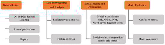
Figure 1.
Flow chart of worldwide EOR screening based on machine learning algorithms.
A comprehensive and reliable EOR dataset is indispensable when applying machine learning algorithms for analysis, as the model’s quality is directly contingent upon the dataset’s integrity [29]. Simultaneously, it is crucial to factor in the outcomes of past EOR technique projects, where the data from successful EOR projects notably contribute to the robustness of classification models.
The dataset is composed of 956 successful EOR projects that were collected around the worldwide oilfields [30,31,32,33,34,35,36,37,38,39,40,41,42,43,44,45,46,47,48,49,50,51,52,53,54,55,56,57,58,59,60,61,62,63,64,65,66,67,68,69,70,71,72,73,74,75,76,77,78,79,80,81,82,83,84,85,86,87,88,89,90,91,92,93,94,95]. Each successful project includes porosity (Φ), permeability (K), depth (D), gravity (γ), temperature (T), viscosity (μ), net thickness (H), and initial oil saturation (S0). After the data collection, the duplicate project information was removed from the dataset and the missing value was filled by the mean value to ensure the high quality of the dataset. To balance the importance of reservoir/fluid parameters, permeability, depth, viscosity, and temperature were transformed to the logarithm scale because these parameters have a large statistical range. Our team has put in the effort to improve the quality of the dataset. This involves analyzing parameter ranges using boxplots to evaluate the maximum and minimum values. These analyzes ensure that parameters remain within reasonable limits and accurately represent most reservoir and fluid characteristics [4,96]. The above data quality assessment work can ensure the feasibility and authenticity of the research.
2.2. Worldwide EOR Project Distributions
The EOR project data is widely distributed. The data sources used in this paper mainly include the United States, Canada, China, and other countries because these countries have high oil demand. Petroleum is mainly distributed in the sedimentary rock layers in the upper crust. Sandstone and carbonatite are usually the main storage rocks for petroleum hydrocarbons. Other types of sedimentary rock layers may also become oil reservoirs. Figure 2 presents the distribution of reservoir lithologies and EOR types. As shown in Figure 2, only 35 project oil production reservoirs are distributed in other rock formations and the rest are distributed in sandstone and carbonatite reservoirs. EOR techniques are divided into three main categories: thermal oil recovery, gas flooding, and chemical flooding. Thermal oil recovery includes steam, combustion, and hot water; gas flooding includes nitrogen miscible flooding, nitrogen immiscible flooding, carbon dioxide miscible flooding, carbon dioxide immiscible flooding, hydrocarbon gas miscible flooding, and hydrocarbon gas immiscible flooding; and chemical flooding includes microbial flooding, surfactant flooding, and polymer flooding. Figure 2 also illustrates that 454 thermal projects has been successfully implemented, which has the highest occupation and account for 47.5% of worldwide EOR projects. Gas flooding has been conducted in 387 reservoirs and chemical flooding was used in 115 reservoirs, which occupies 40.5% and 12%, respectively. In addition, in the thermal method, the steam flooding technique is the most widely used; CO2 miscible/immiscible flooding in gas flooding is a mature gas flooding technique, which is an important application of CO2 and can reduce the content of CO2 in the atmosphere; and among chemical methods, the polymer flooding technique is the most widely used.
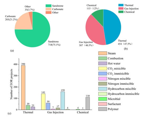
Figure 2.
(a) Distribution of rock formations in the dataset. (b) EOR category distribution of the dataset. (c) EOR technique distribution of the dataset.
Based on the supplementary and complete initial dataset, a frequency distribution analysis of the eight parameters was conducted, as illustrated in Figure 3. The analysis reveals that porosity values for the projects in the dataset predominantly fall between 5% and 40%. The oil layer depth for production is mostly situated more than 100 ft underground, with a significant portion falling within the range of 0 to 12,500 ft. The permeability of the rock formations hosting oil ranges from 0 to 2000 millidarcies (md). Oil viscosity exhibits an uneven distribution, spanning from 0.04 centipoise (cp) to 10,000 cp; around 70% of the samples have a viscosity below 500 cp. The data points with a viscosity greater than 10,000 cp are not shown in the graph due to their limited occurrence. The dataset includes projects involving heavy crude oil and medium crude oil, as well as light crude oil and ultra-light crude oil. Oil temperature varies with depth, primarily falling within the range of 75 °F to 155 °F. The net thickness of the oil layer in the projects generally exceeds 3.4 ft, with most values below 200 ft, indicating a relatively thick and favorable rock formation. The initial oil saturation in the rock formations follows a normal distribution, with the 50% to 70% oil saturation representing the typical range and indicating a relatively high oil content.
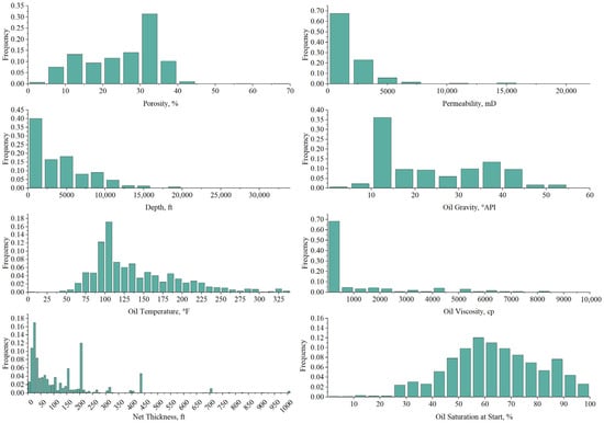
Figure 3.
Distribution of EOR reservoir/fluid parameters.
A scatter plot matrix was utilized to reveal the relationships among reservoir/fluid parameters, as shown in Figure 4. It can be seen from the figure that there is a strong linear relationship between depth and temperature. The deeper the depth, the higher the temperature of the oil; the greater the gravity of the oil, the lower the viscosity; and the deeper the depth, the greater the gravity of the oil.
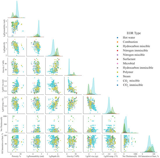
Figure 4.
Scatter matrix plot of EOR project parameters.
After the data analysis, eight reservoir/fluid parameters were selected as the input to the model, which includes: porosity, permeability, depth, oil gravity, oil viscosity, oil temperature, net thickness, and oil saturation at the start of the project. The reasons to choose these parameters are because these parameters are commonly available during the exploration and drilling process, and these parameters could effectively reflect the reservoir and fluid conditions before the implementation of the EOR technique.
3. Methodologies
The performance of the same dataset on different algorithm models are different. In order to select the model with the best prediction accuracy in this dataset, the advanced EOR screening primarily relies on utilizing real-world datasets and employing various machine learning algorithms to establish classification models. Through a review of the literature related to EOR screening and machine learning, we identified five methods, namely random forest, artificial neural networks, naïve Bayes, support vector machines, and decision trees, which have demonstrated excellent performance in classification tasks. Therefore, we chose these algorithms as the tools to implement the dataset in this study. Next, the basic principles and optimization methods of the three algorithms and related evaluation indicators are introduced.
3.1. Decision Trees
The decision trees algorithm is a supervised machine learning algorithm that forms a hierarchical structure by partitioning the data based on features. It selects the best features to split the data, recursively building decision nodes until certain stopping criteria are met. Each leaf node represents a category and the decision tree makes predictions or classifications based on the decision rules along the paths. Feature selection is typically guided by metrics such as information gain or the index, and pruning is applied to prevent overfitting and ensure the model’s generalization capability.
3.2. Random Forest
The random forest algorithm is an ensemble learning algorithm that consists of multiple decision trees [97]. Each decision tree is obtained by random sampling (bagging) the training set, and at each node, it randomly selects a part of the features for division, increasing the diversity of the random forest and reducing the risk of overfitting. The final classification result is the majority vote result of all decision trees.
The random forest algorithm utilizes impurity as the evaluation index of the node quality. The smaller the index, the higher the purity of the dataset and the higher the classification accuracy of the model. The index is defined as:
where is the number of categories, and represents the probability that the sample belongs to the category .
In performing classification tasks, voting is used as a method to select unique classes. Its operation process is as follows. Assuming that there are classifiers and the result of each classifier is , the voting result of the random forest can be expressed as:
where represents the voting result of the random forest, represents the classification label of the classifier, and is the indicator function. When , takes the value of 1, otherwise it takes the value of 0.
Through Equation (2), the number of occurrences of each classification label in the classification records of classifiers can be counted, and then the label with the most occurrences is taken as the final classification result.
As shown in Figure 5, the random forest builds n decision trees to make the corresponding classification results, and then integrates them into a forest. The final classification result is based on the most voting results of each tree. RF selects the divided data for training and prediction and uses the parameter combination with the best performance in the test set for prediction. After multiple adjustments, the model with the best performance in the test set is selected as the final RF model.
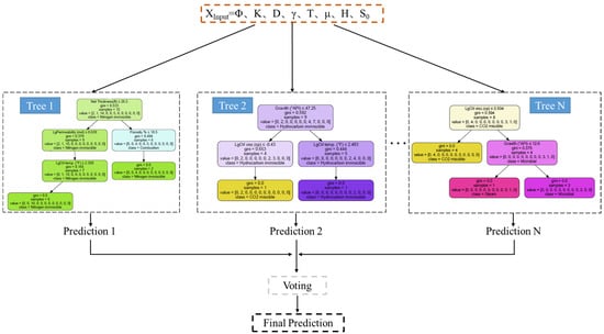
Figure 5.
Schematic diagram of RF.
3.3. Artificial Neural Networks
The ANNs algorithm is a model inspired by the neuron network of the human brain and is used to solve various problems such as classification, regression, and image processing [98]. Its principle is based on information transfer and weight adjustment between neurons. The core is weight. This concept is derived from the simulation of the working principle of the biological nervous system. Artificial neural networks are composed of multiple neurons (simulating biological neurons) distributed in different layers, including the input layer, hidden layer, and output layer. Each neuron receives input from the neuron in the previous layer, performs a weighted sum of the inputs, and then applies an activation function to produce an output. Figure 6 shows the process of the neural networks’ operation and the weight calculation and output of a single neuron.
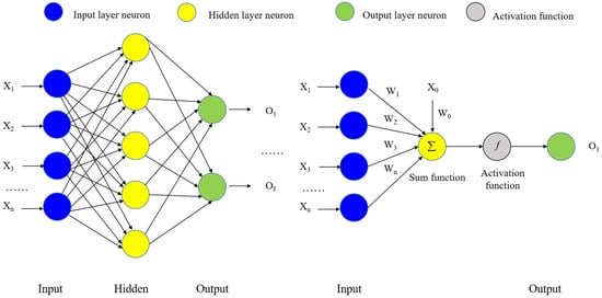
Figure 6.
Flow chart of ANNs and single neuron model.
3.4. Naïve Bayes Classifier
The naïve Bayes classifier, as a classification method based on probability statistics [99], has demonstrated excellent performance and wide applications in many fields and has been applied to classify EOR projects. Its core principle is based on Bayes’ theorem (Equation (3)), which mathematically describes how to estimate the probability of an unknown event given known information. The advantage of the Bayesian classification method is that it can handle uncertainty and can continuously learn and adjust based on the new data to improve the accuracy of classification.
where Cm represents the category, X stands for a sample with features (x1, x2, …… xn), p(Cm) is the Priori probability, p(X) is the total probability of the occurrence of data X, p(Cm|X) is the Posterior probability, and p(X|Cm) indicates the probability of observing data X under the assumption that Cm is established.
3.5. Support Vector Machines
In classification problems, the goal of support vector machines is to find an optimal hyperplane that separates the data of different categories. Its basic principle is to find an optimal decision boundary (or hyperplane) between data points so that the data points of different categories are the farthest away from the boundary. This article uses a nonlinear support vector machine. If the sample can be mapped from the original space to a higher-dimensional space, then a hyperplane can be found to divide the sample in the new feature space and converted into a linearly separable support vector machine.
3.6. Evaluation Index
The confusion matrix is a commonly used performance evaluation method in machine learning, which is mainly used to measure the performance of classification models. It compares the real label of the sample with the predicted label of the classifier by statistically analyzing the classification results of the classifier and then calculating the classification precision, recall, accuracy, F1 Score, and other indicators of the classifier, of which the calculation formula of the index is shown in Equations (4)–(6).
Precision refers to the proportion of samples predicted to be positive that are actually positive.
Recall refers to the proportion of samples that are predicted to be positive among the samples that are actually positive.
Accuracy refers to the proportion of correctly classified positive samples among all samples classified as positive samples.
where TP (True Positive) represents the number of samples that are actually positive and predicted to be positive, FP (False Positive) stands for the number of samples that are actually negative and predicted to be positive, FN (False negative) is the number of samples that are actually positive and predicted to be negative, and TN (True negative) is the number of samples that are actually negative examples and predicted to be negative.
In practical problems, we often consider the precision (P) and the recall (R) comprehensively, that is, the F1Score, which is defined as the harmonic mean of the precision rate and the recall rate.
To better display the classification results of the EOR technique, the confusion matrix is used as a visual solution.
The schematic diagram of the confusion matrix is shown in Figure 7, which means that the samples whose instances are positive examples are all correctly predicted as positive examples, and the samples whose instances are negative examples are all correctly predicted as negative examples. This is the ideal confusion matrix.
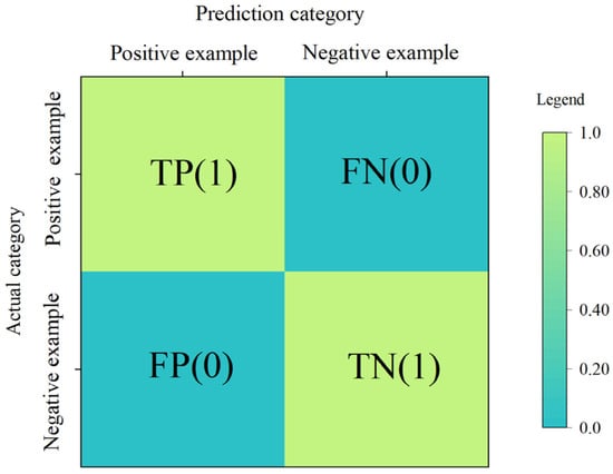
Figure 7.
Schematic diagram of a confusion matrix.
3.7. Optimization Methods
Grid search and random search are two commonly used hyper-parameter optimization methods in machine learning. Grid search is a method of searching for the best hyper parameters by enumerating all possible combinations of hyper parameters. It finds the best combination by performing a systematic search in a given grid of hyper parameters. Since it needs to try all possible combinations, it is computationally expensive, especially when the number of hyper parameters is large.
On the other hand, random search is a more flexible approach that randomly selects a set of hyper parameters in a given hyper-parameter space and evaluates them against a given performance metric.
Experiments have shown that random search could have better performance than grid search because random search can search continuous values and can set a larger search space, so there is a chance to obtain a better model [100]. The relevant experimental results are shown in Figure 8, in the same nine-sampled search, where the grid search was sampled only three times for important parameters, compared to nine random searches. In addition, for cases where only a few hyper parameters play a decisive role, random search is more efficient for searching important parameters. Previous research in the field of machine learning has indicated minimal disparities in the final parameter prediction accuracy between the two methods after many iterations.
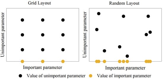
Figure 8.
Experimental distribution for grid search and random search.
To select an appropriate hyper-parameter optimization method, random search and grid optimization are plotted on the epoch parameter optimization process in the EOR project dataset, as shown in Figure 9, through the comparison of the above grid search and random search methods, according to the size of the dataset and the optimization space of parameters. Under the same conditions, random search reaches higher accuracy faster than grid search. Although other methods such as automated hyper-parameter tuning, Bayesian optimization, genetic algorithms, and artificial neural networks tuning are also highly effective, in the context of our study, random search was considered an appropriate and practical choice. Random search does not rely on a priori knowledge and therefore is not affected by the initial parameter choice, which can lead to better results in some cases. Moreover, random search can explore a wider hyper-parameter space with limited computing resources, improving the chance of finding a satisfactory solution. In addition, in our specific dataset, we conducted multiple experiments and proved that random search performed well under our dataset and model architecture, so we finally chose random search as the method for hyper-parameter optimization.
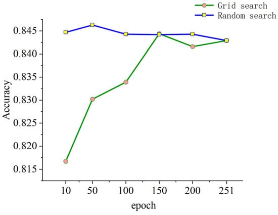
Figure 9.
Comparison of random search and grid search methods in random forest optimization.
4. EOR Screening Modeling
4.1. Modeling
In this paper, according to the random state of 42, the dataset is divided into an 80% training set and a 20% test set. The scale of the training set and test set is shown in Table 2.
Table 2.
The size of the training set and test set.
At this stage, the default parameters are used for modeling and their related parameters are shown in Table 3, Table 4 and Table 5. These models are established according to the random state of 42 and the accuracy of the training set and test set under the model is obtained.
Table 3.
Default parameters for random forest models.
Table 4.
Default parameters for ANNs models.
Table 5.
Default parameters for SVM models.
Table 6 shows the store prediction effects of the three algorithms on the training set and test set. Under these models, the prediction accuracy of the random forest model is better. The prediction accuracy of the training set is 99.34% and the prediction accuracy of the test set is 88.54%. There is a certain degree of overfitting in the training set and the accuracy of the test set needs to be improved. Therefore, the next step is to improve the prediction accuracy of the model by optimizing the hyper parameters.
Table 6.
Accuracy of different algorithms on training set and test set before optimization.
4.2. Hyper-Parameters Optimization
After the comparison in Figure 9, considering the hyper-parameter space and the dataset size, we utilized random search to optimize the hyper parameters of RF, ANNs, and SVM. The optimal hyper-parameter combinations were determined based on the accuracy of the test set, serving as the performance metric. We defined the range of hyper parameters for both RF, ANNs, and SVM models based on the dataset’s size and the model’s characteristics. Within these predefined ranges, we systematically explored various parameter combinations to identify the optimal set. The detailed parameter settings can be found in Table 7, Table 8 and Table 9. The main hyper parameter combinations obtained using random search are shown in Table 10, Table 11 and Table 12.
Table 7.
Range of random forest hyper parameters.
Table 8.
Range of ANNs hyper parameters.
Table 9.
Range of SVM hyper parameters.
Table 10.
Hyper-parameter values of RF after random search optimization.
Table 11.
Hyper-parameter values of ANNs after random search optimization.
Table 12.
Hyper-parameter values of SVM after random search optimization.
The Bayesian network classification model uses Bayes’ theorem to estimate the conditional probability distribution of the given input data. The structure of the Bayesian network is represented by a directed acyclic graph and the parameters are learned from the training data. Therefore, unlike many other machine learning models, the structure and parameter settings of Bayesian networks do not depend on the hyper parameters. As a result, the Bayesian network is not optimized.
Random forest is composed of multiple decision trees; in the optimization process, we use RF, ANNs, and SVM algorithms to obtain the optimal hyper-parameter combination via random search. After the RF, ANNs, and SVM model is randomly searched to determine the hyper-parameter combination, the divided 20% dataset is used as the test set. There are 10 EOR techniques in the test set, and the classifier of RF, ANNs, and SVM modeling is verified by using the optimized hyper-parameter combination.
4.3. Results and Discussion
Among these five algorithms, random forest is an ensemble method based on decision trees. After optimization, the SVM algorithm exhibited the lowest modeling accuracy. Consequently, our subsequent analysis will focus on the results obtained from RF, ANNs, and naïve Bayes. Table 13 shows the accuracy of classification using optimized parameters. In this study, the ANNs model is more suitable for the training and learning of big data. The Bayesian network model has low classification accuracy due to the phenomenon of classification imbalance. The RF classification model has the highest accuracy. The RF, ANNs, and naïve Bayes classification models were evaluated according to the precision, recall, accuracy, and F1Score.
Table 13.
Accuracy of different algorithms on training set and test set after optimization.
Using the hyper-parameter combination found via a random search, the random forest model was established to predict the test set containing 192 samples, where the accuracy increased by 2.61% from 88.54% to 91.15%.
After the random forest model determines the combination of hyper parameters via the random search, classes 0, 1, 2, 3, 4, 5, 6, 7, 8, 9, 10, and 11 correspond to steam flooding, combustion, hot water flooding, and CO2 miscible flooding, CO2 immiscible flooding, nitrogen miscible flooding, nitrogen immiscible flooding, hydrocarbon miscible flooding, hydrocarbon immiscible flooding, microbial flooding, surfactant flooding, and polymer flooding. The prediction effects of the optimized random forest model, ANNs model, and Bayesian model on the test set are shown in Table 14, Table 15 and Table 16. The prediction effect of each specific EOR technique is displayed. To express the effect more intuitively, it is visualized via the receiver operating characteristic (ROC) curve and the confusion matrix.
Table 14.
Optimized random forest model classification’s Precision, Recall, and F1 Score.
Table 15.
Optimized ANNs model classification’s Precision, Recall, and F1 Score.
Table 16.
Naïve Bayes model classification’s Precision, Recall, and F1 Score.
The classification results of the test set are visualized via the ROC curve, as shown in Figure 10, Figure 11 and Figure 12. It can be seen that the ROC curve of the random forest model performs best, mostly concentrated in the upper left corner, which means the prediction accuracy is good. The conclusion that the test area under the ROC curve (AUC) values are all greater than 0.97 is obtained in ROC based on RF. Among them, the AUC value of the EOR technique not included in the test set is set to 0, indicating that the optimized random forest classifier has very good performance in the classification prediction of multiple EOR techniques and that its high precision, high efficiency, and high generalization performance can provide technical support for the EOR screening of field reservoirs.
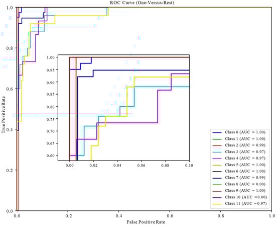
Figure 10.
ROC curve of the test set based on RF.
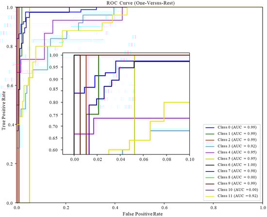
Figure 11.
ROC curve of the test set based on ANNs.
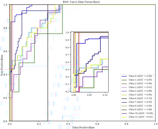
Figure 12.
ROC curve of the test set based on naïve Bayes classifier.
The confusion matrices in Figure 13, Figure 14 and Figure 15 illustrate the prediction results of the test set, where the predictions are presented by different EOR techniques (left) and EOR categories (right), respectively. In the comparison of results, we can see that random forest has the best prediction accuracy for EOR sample classification in the test set. The results show that the test set contains ten EOR techniques, covering three EOR categories: thermal flooding, gas injection flooding, and chemical flooding. In the prediction of the thermal flooding category, steam flooding and combustion reached an accuracy of 1. Due to the small number of samples, techniques such as hot water were wrongly predicted as steam flooding, which still belonged to the thermal flooding category, which does not have significant influence on the enhanced oil recovery in the field of engineering applications. For gas injection flooding, the prediction accuracy of the hydrocarbon gas miscible flooding technique is 92%, and in the prediction category of the CO2 miscible flooding and CO2 immiscible flooding technique, more than 85% of the probability predictions are still in the gas drive technique. Due to the small number of actual samples and the prediction accuracy of nitrogen miscible flooding and nitrogen immiscible flooding, the impact on the overall prediction results of gas flooding is small. After the random forest model prediction, 96% of the samples are predicted to be in the gas drive category. Due to the size of the data and reality, a small number of samples are predicted to be in the thermal drive category. In chemical flooding, only microbial flooding and polymer flooding techniques are included. Among the 26 samples, only three samples are predicted to be other types, which achieves an 88% prediction accuracy. The stability and reliability of the aforementioned model in classification tasks are intricately tied to the quality of the dataset we meticulously curated. The authenticity and precision of the data are pivotal, rendering the machine learning model practically feasible. Furthermore, the utilization of the RF algorithm, a well-established and mature classification technique, contributes significantly to the model’s stability in operations.
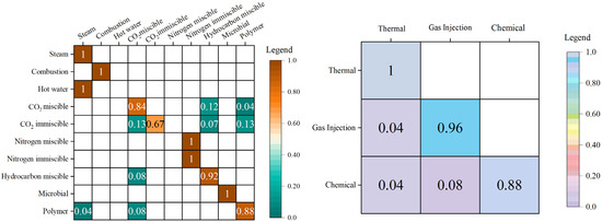
Figure 13.
Confusion matrices for the test set (RF).
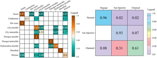
Figure 14.
Confusion matrices for the test set (ANNs).
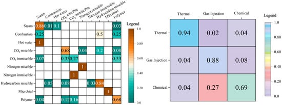
Figure 15.
Confusion matrices for the test set (naïve Bayes).
The visualization of the classification results of the random forest classifier for the test set via the ROC curve and the confusion matrix demonstrates the optimized model’s high accuracy in predicting EOR techniques. By employing the RF algorithm as the core of the prediction system and storing the acquired drilling data in the dataset, an appropriate EOR technique tailored to the specific reservoir characteristics can be determined. Given that the parameter distribution of the collected dataset spans across a significant portion of reservoir variations, the classification model established using this dataset holds the potential for widespread application and implementation. This approach assists reservoir engineers in decision making, saving time and economic costs by streamlining the process of identifying the most effective techniques for enhanced oil recovery.
5. Conclusions
Due to the efficient and accurate nature of machine learning algorithms, we have integrated them into the process of selecting EOR techniques in reservoir engineering. Aiming at the EOR screening scheme, this study developed several prediction mechanisms with machine learning algorithm models as the core. The main results are as follows.
- We have compiled a comprehensive dataset comprising 956 successful global EOR projects, incorporating essential reservoir fluid attributes and supplemented with complete net thickness information.
- We established models based on RF, ANNs, naïve Bayes, SVM, and decision trees to predict EOR project categories for the given input parameters. Subsequently, we first compared the accuracy of these algorithms and we conducted a comprehensive analysis and comparison of RF, ANNs, and naïve Bayes, evaluating the models from the perspectives of precision, recall, and the F1 score.
- In the process of model optimization, we considered the scale of the dataset and various optimization techniques. Consequently, we chose random search as the method to determine the optimal parameters.
- After the comparison of these models, the RF model has the highest accuracy on the test set, reaching 91.15%, which provides an important basis for the real-time and efficient enhanced oil recovery screening decision of the oil field.
- Overall, this study provides reservoir engineers with a convenient and quick way to confirm the EOR technique solution suitable for the reservoir. In future research, advanced deep learning techniques such as recurrent neural networks (RNNs) and convolutional neural networks (CNNs) can be applied in modeling EOR screening to enhance the predictive accuracy of EOR screening models. Furthermore, there is a need for research focusing on the environmental and economic implications of different EOR methods. Taking this into account in EOR modeling, scholars can make a significant contribution to the development of EOR modeling and promote implementing oil and sustainable solutions in the oil and gas industry.
Author Contributions
Methodology, N.Z.; Validation, S.S., H.W. and M.Z.; Resources, A.Z.; Data curation, P.W.; Writing—original draft, S.S.; Writing—review & editing, N.Z.; Funding acquisition, S.J. All authors have read and agreed to the published version of the manuscript.
Funding
This research was supported by the National Science Foundation of China (grants 52204041 and 71971130), Natural Science Foundation of Shandong Province (grant ZR2021QF076), Project of Shandong Province Higher Educational “Youth Innovation Science and Technology Plan” (grant 2021KJ060), and Taishan Scholar Young Talent Program (No.tsqn202306202). And the APC was funded by Natural Science Foundation of Shandong Province (grant ZR2021QF076).
Institutional Review Board Statement
Not applicable.
Informed Consent Statement
Not applicable.
Data Availability Statement
The data presented in this study are available on request from the corresponding author. The data are not publicly available due to privacy.
Acknowledgments
The authors acknowledge Natural Science Foundation of Shandong Province.
Conflicts of Interest
Author Peng Wang was employed by the company Changqing Oilfield Branch of PetroChina. The remaining authors declare that the research was conducted in the absence of any commercial or financial relationships that could be construed as a potential conflict of interest.
Nomenclature
| EOR | Enhanced oil recovery |
| RF | Random forest |
| ANNs | Artificial neural networks |
| SVM | Support vector machines |
| AI | Artificial Intelligence |
| ROC | Receiver operating characteristic |
| AUC | Area under the ROC Curve |
| TP | True Positive |
| FP | False Positive |
| FN | False Negative |
| TN | True Negative |
References
- Heidari, H.; Akbari, M.; Souhankar, A.; Hafezi, R. Review of global energy trends towards 2040 and recommendations for Iran oil and gas sector. Int. J. Environ. Sci. Technol. 2022, 19, 8007–8018. [Google Scholar] [CrossRef]
- Niu, J.; Liu, Q.; Lv, J.; Peng, B. Review on microbial enhanced oil recovery: Mechanisms, modeling and field trials. J. Pet. Sci. Eng. 2020, 192, 107350. [Google Scholar] [CrossRef]
- U.S. Department of Energy. Enhanced Oil Recovery. Available online: https://www.energy.gov/fecm/enhanced-oil-recovery (accessed on 23 October 2023).
- Zhang, N.; Wei, M.Z.; Fan, J.Y.; Aldhaheri, M.; Zhang, Y.D.; Bai, B.J. Development of a hybrid scoring system for EOR screening by combining conventional screening guidelines and random forest algorithm. Fuel 2019, 256, 115915. [Google Scholar] [CrossRef]
- Cheraghi, Y.; Kord, S.; Mashayekhizadeh, V. Application of machine learning techniques for selecting the most suitable enhanced oil recovery method; challenges and opportunities. J. Pet. Sci. Eng. 2021, 205, 108761. [Google Scholar] [CrossRef]
- Taber, J.J.; Martin, F.D.; Seright, R.J. EOR screening criteria revisited—Part 1: Introduction to screening criteria and enhanced recovery field projects. SPE Reserv. Eng. 1997, 12, 189–198. [Google Scholar] [CrossRef]
- Al Adasani, A.; Bai, B. Engineering, Analysis of EOR projects and updated screening criteria. J. Pet. Sci. Eng. 2011, 79, 10–24. [Google Scholar] [CrossRef]
- Hama, M.Q.; Wei, M.; Saleh, L.D.; Bai, B. Updated screening criteria for steam flooding based on oil field projects data. In Proceedings of the SPE Heavy Oil Conference-Canada, Calgary, AB, Canada, 10–12 June 2014. [Google Scholar]
- Saleh, L.D.; Wei, M.; Bai, B. Data Analysis and Updated Screening Criteria for Polymer Flooding Based on Oilfield Data. SPE Reserv. Eval. Eng. 2014, 17, 15–25. [Google Scholar] [CrossRef]
- Aldhaheri, M.; Wei, M.; Zhang, N.; Bai, B. Engineering, Field design guidelines for gel strengths of profile-control gel treatments based on reservoir type. J. Pet. Sci. Eng. 2020, 194, 107482. [Google Scholar] [CrossRef]
- Pirizadeh, M.; Alemohammad, N.; Manthouri, M.; Pirizadeh, M. A new machine learning ensemble model for class imbalance problem of screening enhanced oil recovery methods. J. Pet. Sci. Eng. 2021, 198, 108214. [Google Scholar] [CrossRef]
- Alvarado, V.; Ranson, A.; Hernandez, K.; Manrique, E.; Matheus, J.; Liscano, T.; Prosperi, N. Selection of EOR/IOR opportunities based on machine learning. In Proceedings of the European Petroleum Conference, Aberdeen, UK, 29–31 October 2002. [Google Scholar]
- Siena, M.; di Milano, P.; Guadagnini, A.; Rossa, E.D.; Lamberti, A.; Masserano, F.; Rotondi, M. A New Bayesian Approach for Analogs Evaluation in Advanced EOR Screening. In Proceedings of the EUROPEC 2015, Madrid, Spain, 1–4 June 2015. [Google Scholar]
- Siena, M.; Guadagnini, A.; Rossa, E.D.; Lamberti, A.; Masserano, F.; Rotondi, M. A Novel Enhanced-Oil-Recovery Screening Approach Based on Bayesian Clustering and Principal-Component Analysis. SPE Reserv. Eval. Eng. 2016, 19, 382–390. [Google Scholar] [CrossRef]
- Zhang, N.; Wei, M.Z.; Bai, B.J.; Wang, X.P.; Hao, J.; Jia, S. Pattern Recognition for Steam Flooding Field Applications Based on Hierarchical Clustering and Principal Component Analysis. ACS Omega 2022, 7, 18804–18815. [Google Scholar] [CrossRef] [PubMed]
- Giro, R.; Lima Filho, S.P.; Neumann Barros Ferreira, R.; Engel, M.; Steiner, M.B. Artificial intelligence-based screening of enhanced oil recovery materials for reservoir-specific applications. In Proceedings of the Offshore Technology Conference Brasil, Rio de Janeiro, Brazil, 29–31 October 2019. [Google Scholar]
- Khazali, N.; Sharifi, M.; Ahmadi, M.A. Application of fuzzy decision tree in EOR screening assessment. J. Pet. Sci. Eng. 2019, 177, 167–180. [Google Scholar] [CrossRef]
- Muñoz Vélez, E.A.; Romero Consuegra, F.; Berdugo Arias, C.A. EOR screening and early production forecasting in heavy oil fields: A machine learning approach. In Proceedings of the SPE Latin American and Caribbean Petroleum Engineering Conference, Bogotá, Colombia, 17–19 March 2020. [Google Scholar]
- Cheraghi, Y.; Kord, S.; Mashayekhizadeh, V. A two-stage screening framework for enhanced oil recovery methods, using artificial neural networks. Neural Comput. Appl. 2023, 35, 17077–17094. [Google Scholar] [CrossRef]
- Keil, T.; Kleikamp, H.; Lorentzen, R.J.; Oguntola, M.B.; Ohlberger, M. Adaptive machine learning-based surrogate modeling to accelerate PDE-constrained optimization in enhanced oil recovery. Adv. Comput. Math. 2022, 48, 73. [Google Scholar] [CrossRef]
- Prudencio, G.; Celis, C.; Armacanqui, J.S.; Sinchitullo, J. Development of an evolutionary artificial neural network-based tool for selecting suitable enhanced oil recovery methods. J. Braz. Soc. Mech. Sci. Eng. 2022, 44, 121. [Google Scholar] [CrossRef]
- Koray, A.-M.; Bui, D.; Ampomah, W.; Appiah Kubi, E.; Klumpenhower, J. Application of Machine Learning Optimization Workflow to Improve Oil Recovery. In Proceedings of the SPE Oklahoma City Oil and Gas Symposium, Oklahoma City, OK, USA, 17–19 April 2023. [Google Scholar]
- Abdullah, M.B.; Delshad, M.; Sepehrnoori, K.; Balhoff, M.T.; Foster, J.T.; Al-Murayri, M.T. Physics-Based and Data-Driven Polymer Rheology Model. SPE J. 2023, 28, 1857–1879. [Google Scholar] [CrossRef]
- Sinha, U.; Dindoruk, B.; Soliman, M.J. Prediction of CO2 Minimum Miscibility Pressure Using an Augmented Machine-Learning-Based Model. SPE J. 2021, 26, 1666–1678. [Google Scholar] [CrossRef]
- Mahdaviara, M.; Sharifi, M.; Ahmadi, M. Toward evaluation and screening of the enhanced oil recovery scenarios for low permeability reservoirs using statistical and machine learning techniques. Fuel 2022, 325, 124795. [Google Scholar] [CrossRef]
- Ibrahim, A.F.; Elkatatny, S. Application of Machine Learning to Predict Shale Wettability. In Proceedings of the Offshore Technology Conference, Rio de Janeiro, Brazil, 24–26 October 2023. [Google Scholar]
- Pooladi-Darvish, M.; Tabatabaie, S.H.; Rodriguez Cadena, C. Development of a Machine Learning Technique in Conjunction with Reservoir Complexity Index to Predict Recovery Factor Using Data from 18,000 Reservoirs. In Proceedings of the ADIPEC 2022, Abu Dhabi, United Arab Emirates, 31 October–3 November 2022. [Google Scholar]
- Yao, Y.; Qiu, Y.; Cui, Y.; Wei, M.Z.; Bai, B.J. Insights to surfactant huff-puff design in carbonate reservoirs based on machine learning modeling. Chem. Eng. J. 2023, 451, 16. [Google Scholar] [CrossRef]
- Huang, S.H.; Tian, L.; Zhang, J.S.; Chai, X.L.; Wang, H.L.; Zhang, H.L. Support Vector Regression Based on the Particle Swarm Optimization Algorithm for Tight Oil Recovery Prediction. ACS Omega 2021, 6, 32142–32150. [Google Scholar] [CrossRef]
- Aalund, L.R. Annual production report: EOR projects decline but CO2 pushes up production. Oil Gas J. 1988, 86, 33–74. [Google Scholar]
- Alvarado, V.; Manrique, E.J.E. Enhanced oil recovery: An update review. Energies 2010, 3, 1529–1575. [Google Scholar] [CrossRef]
- Ampomah, W.; Balch, R.; Grigg, R.; Will, R.; Dai, Z.; White, M. Farnsworth field CO2-EOR project: Performance case history. In Proceedings of the SPE Improved Oil Recovery Conference, Tulsa, OK, USA, 11–13 April 2016; p. SPE-179528-MS. [Google Scholar]
- Aryana, S.A.; Barclay, C.; Liu, S. North cross devonian unit-a mature continuous CO2 flood beyond 200% HCPV injection. In Proceedings of the SPE Annual Technical Conference and Exhibition, Amsterdam, The Netherlands, 27–29 October 2014; p. SPE-170653-MS. [Google Scholar]
- Bangia, V.; Yau, F.; Hendricks, G.R. Reservoir performance of a gravity-stable, vertical CO2 miscible flood: Wolfcamp Reef Reservoir, Wellman Unit. SPE Reserv. Eng. 1993, 8, 261–269. [Google Scholar] [CrossRef]
- Barrett, D.; Harpole, K.; Zaaza, M. Reservoir Data Pays Off: West Seminole San Andres Unit, Gaines County, Texas. In Proceedings of the SPE Annual Fall Technical Conference and Exhibition, Denver, CO, USA, 9–12 October 1977. [Google Scholar]
- Bass, N.W. Subsurface Geology and Oil and Gas Resources of Osage County, Oklahoma; US Government Printing Office: Washington, DC, USA, 1938; Volume 900. [Google Scholar]
- Bellavance, J. Dollarhide Devonian CO2 Flood: Project performance review 10 years later. In Proceedings of the Permian Basin Oil and Gas Recovery Conference, Midland, TX, USA, 27–29 March 1996. [Google Scholar]
- Bleakley, W.B. Survey pinpoints recovery projects. Oil Gas J. 1971, 69, 87–91. [Google Scholar]
- Bleakley, W.B. Production report: Journal survey shows recovery projects up. Oil Gas J. 1974, 72, 72–78. [Google Scholar]
- Brinkman, F.; Kane, T.; McCullough, R.; Miertschin, J.J. Engineering, Use of full-field simulation to design a miscible CO2 flood. SPE Reserv. Eval. Eng. 1999, 2, 230–237. [Google Scholar] [CrossRef]
- Brinlee, L.D.; Brandt, J.A. Planning and development of the Northeast Purdy Springer CO2 miscible project. In Proceedings of the SPE Annual Technical Conference and Exhibition 1982, New Orleans, LA, USA, 26–29 September 1982; p. SPE-11163-MS. [Google Scholar]
- Brokmeyer, R.; Borling, D.; Pierson, W. Lost Soldier Tensleep CO2 Tertiary Project, Performance Case History; Bairoil, Wyoming. In Proceedings of the SPE Permian Basin Oil and Gas Recovery Conference, Midland, TX, USA, 27–29 March 1996; p. SPE-35191-MS. [Google Scholar]
- Cain, M. Brookhaven Field: Conformance Challenges in an Active CO2 Flood. In Proceedings of the 16th Annual CO2 Flooding Conference, Midland, TX, USA, 9–10 December 2010; pp. 9–10. [Google Scholar]
- Chen, T.; Kazemi, H.; Davis, T. Integration of reservoir simulation and time-lapse seismic in Delhi Field: A continuous CO2 injection EOR project. In Proceedings of the SPE Improved Oil Recovery Symposium, Tulsa, OK, USA, 12–16 April 2014. [Google Scholar]
- Demirdal, A.; Derya, G. Role of Catalytic Agents on Combustion Front Propagation in Porous Media. Master’s Thesis, Department of Civil and Environmental Engineering, University of Alberta, Edmonton, AB, Canada, 2007. [Google Scholar]
- Denney, D. Improved-recovery processes and effective reservoir management maximize oil recovery Salt Creek. J. Pet. Technol. 2003, 55, 42. [Google Scholar] [CrossRef]
- Dutton, S.P.; Flanders, W.A.; Barton, M.D. Reservoir characterization of a Permian deep-water sandstone, East Ford field, Delaware basin, Texas. AAPG Bull. 2003, 87, 609–627. [Google Scholar] [CrossRef]
- Eaves, E. Citronelle oil field, mobile County, Alabama. In M 24: North American Oil and Gas Fields; AAPG: Tulsa, OK, USA, 1976. [Google Scholar]
- Eisterhold, J.F.; Armstrong, R., Jr. Utilization of an oil spill cooperative to meet worst case discharge requirements. In Proceedings of the Offshore Technology Conference, Houston, TX, USA, 1–4 May 2000; OTC: Boca Raton, FL, USA, 2000; p. OTC-11987-MS. [Google Scholar]
- Flanders, W.A.; Stanberry, W.A.; Martinez, M. CO2 injection increases Hansford Marmaton production. J. Pet. Technol. 1990, 42, 68–73. [Google Scholar] [CrossRef]
- Frascogna, X.M. Mallalieu Field Lincoln County Mississippi. In Mesozoic-Paleozoic Producing Areas of Mississippi and Alabama; AAPG: Tulsa, OK, USA, 1957. [Google Scholar]
- Gingrich, D.; Knock, D.; Masters, R. Geophysical interpretation methods applied at Alpine oil field: North Slope, Alaska. Geophysics 2001, 20, 730–738. [Google Scholar] [CrossRef]
- Hervey, J.; Iakovakis, A.C. Performance Review off a Miscible CO2 Tertiary Project: Rangely Weber Sand Unit, Colorado. SPE Reserv. Eng. 1991, 6, 163–168. [Google Scholar] [CrossRef]
- Hoiland, R.; Joyner, H.; Stalder, J. Case history of a successful rocky mountain pilot CO2 flood. In Proceedings of the SPE Enhanced Oil Recovery Symposium, Tulsa, OK, USA, 20–23 April 1986. [Google Scholar]
- Holtz, M.H. Summary of Gulf Coast Sandstone CO2 EOR Flooding Application and Response. In Proceedings of the SPE Improved Oil Recovery Conference, Tulsa, OK, USA, 20–23 April 2008; p. SPE-113368-MS. [Google Scholar]
- Jasek, D.; Frank, J.; Mathis, L.; Smith, D. Goldsmith San Andres unit CO2 pilot-design, implementation, and early performance. In Proceedings of the SPE Annual Technical Conference and Exhibition, New Orleans, LA, USA, 27–30 September 1998; p. SPE-48945-MS. [Google Scholar]
- Keeling, R. CO2 Miscible flooding evaluation of the south welch unit, welch san andres field. In Proceedings of the SPE Enhanced Oil Recovery Symposium, Tulsa, OK, USA, 15–18 April 1984. [Google Scholar]
- Kirkpatrick, R.; Flanders, W.; DePauw, R. Performance of the Twofreds CO2 injection project. In Proceedings of the SPE Annual Technical Conference and Exhibition, Las Vegas, NV, USA, 22–26 September 1985; p. SPE-14439-MS. [Google Scholar]
- Kleinstelber, S.W. The Wertz Tensleep CO2 flood: Design and initial performance. J. Pet. Technol. 1990, 42, 630–636. [Google Scholar] [CrossRef]
- Koottungal, L. Miscible CO2 now eclipses steam in US EOR production. Oil Gas J. 2012, 110, 56–69. [Google Scholar]
- Koottungal, L. Survey: Miscible CO2 continues to eclipse steam in US EOR production. Oil Gas J. 2014, 112, 78–91. [Google Scholar]
- Kovarik, M.; Prasad, R.; Waddell, W.; Watts, G. North Dollarhide (Devonian) Unit: Reservoir Characterization and CO2 Feasibility Study. In Proceedings of the Permian Basin Oil and Gas Recovery Conference, Midland, TX, USA, 16–18 March 1994; OnePetro: Richardson, TX, USA, 1994. [Google Scholar]
- Leonard, J. EOR set to make significant contribution. Oil Gas J. 1984, 82, 83–105. [Google Scholar]
- Leonard, J. Steam dominates enhanced oil recovery. Oil Gas J. 1986, 80, 139–159. [Google Scholar]
- Leonard, J. Increased rate of EOR brightens outlook. Oil Gas J. 1986, 84, 71–89. [Google Scholar]
- Linroth, M.A.; Rickard, A.E. Pressure and Rate Rebalancing to Improve Recovery in a Miscible CO2 EOR Project. In Proceedings of the SPE Improved Oil Recovery Conference, Tulsa, OK, USA, 12–16 April 2014; p. SPE-169175-MS. [Google Scholar]
- Marchant, L.; Hamke, J. Nitrogen In Clear Creek And Charlson Fields, North Dakota. In Proceedings of the SPE Rocky Mountain Petroleum Technology Conference/Low-Permeability Reservoirs Symposium, Casper, WY, USA, 24–25 May 1964; p. SPE-836-MS. [Google Scholar]
- Masoner, L.; Wackowski, R.K. Rangely weber sand unit CO2 project update. SPE Reserv. Eng. 1995, 10, 203–207. [Google Scholar] [CrossRef]
- Matheny, S.L., Jr. EOR methods help ultimate recovery. Oil Gas J. 1980, 78, 79–124. [Google Scholar]
- Melzer, L.S. Stranded Oil in the Residual Oil Zone. Melzer Consulting Prepared for Advanced Resources International and the US Department of Energy: Office of Fossil Energy-Office of Oil and Natural Gas, 2006: 91. Available online: https://www.researchgate.net/profile/Steve-Melzer/publication/323583727_STRANDED_OIL_IN_THE_RESIDUAL_OIL_ZONE_Prepared_for_Advanced_Resources_International_and_US_Department_of_Energy_Office_of_Fossil_Energy-Office_of_Oil_and_Natural_Gas/links/5a9ec0b845851543e6341f4b/STRANDED-OIL-IN-THE-RESIDUAL-OIL-ZONE-Prepared-for-Advanced-Resources-International-and-US-Department-of-Energy-Office-of-Fossil-Energy-Office-of-Oil-and-Natural-Gas.pdf (accessed on 8 November 2023).
- Meyers, B.D.; Daggett, L.P. Pecos River water treatment for water injection. In Proceedings of the SPE Annual Technical Conference and Exhibition, Denver, CO, USA, 9–12 October 1977; SPE: Richardson, TX, USA, 1977; p. SPE-6883-MS. [Google Scholar]
- Moritis, G. CO2 and HC injection lead EOR production increase. Oil Gas J. 1990, 88, 49–82. [Google Scholar]
- Moritis, G. EOR increases 24% worldwide; claims 10% of US production. Oil Gas J. 1992, 90. [Google Scholar]
- Moritis, G. EOR dips in US but remains a significant factor. Oil Gas J. 1994, 92. [Google Scholar]
- Moritis, G. New technology, improved economics boost EOR hopes. Oil Gas J. 1996, 94. [Google Scholar]
- Moritis, G. More CO2 floods start up in West Texas. Oil Gas J. 1996, 94. [Google Scholar]
- Moritis, G. EOR oil production up slightly. Oil Gas J. 1998, 96, 49–56. [Google Scholar]
- Moritis, G. EOR weathers low oil prices. Oil Gas J. 2000, 98, 39. [Google Scholar]
- Moritis, G. EOR continues to unlock oil resources. Oil Gas J. 2004, 102, 45. [Google Scholar]
- Moritis, G. CO2 injection gains momentum. Oil Gas J. 2006, 104, 37. [Google Scholar]
- Moritis, G. More US EOR projects start but EOR production continues decline. Oil Gas J. 2008, 106, 41–59. [Google Scholar]
- Moritis, G. CO2 miscible, steam dominate enhanced oil recovery processes. Oil Gas J. 2010, 108, 36–40. [Google Scholar]
- Noran, D. Enhanced oil recovery action is worldwide. Production report. Oil Gas J. 1976, 5, 107–131. [Google Scholar]
- Olea, R.A. CO2 retention values in enhanced oil recovery. J. Pet. Sci. Eng. 2015, 129, 23–28. [Google Scholar] [CrossRef]
- Palmer, F.; Nute, A.; Peterson, R.L. Implementation of a gravity-stable miscible CO2 flood in the 8000 foot sand, Bay St. Elaine Field. J. Pet. Technol. 1984, 36, 101–110. [Google Scholar] [CrossRef]
- Peterson, C.A.; Pearson, E.J.; Chodur, V.T.; Periera, C. Beaver Creek Madison CO2 Enhanced Oil Recovery Project Case History; Riverton, Wyoming. In Proceedings of the SPE Improved Oil Recovery Conference, Tulsa, OK, USA, 14–18 April 2012; p. SPE-152862-MS. [Google Scholar]
- Poole, E. Evaluation and Implementation of CO2 Injection at the Dollarhide Devonian Unit. In Proceedings of the SPE Permian Basin Oil and Gas Recovery Conference, Midland, TX, USA, 10–11 March 1988; p. SPE-17277-MS. [Google Scholar]
- Potter, G.C. DM Cogdell Lease, Kent County, Texas. In Abilene Geological Society; AAPG: Tulsa, OK, USA, 1952. [Google Scholar]
- Ring, J.; Smith, D. An overview of the North Ward Estes CO2 flood. In Proceedings of the SPE Annual Technical Conference and Exhibition, Dallas, TX, USA, 22–25 October 1995; p. SPE-30729-MS. [Google Scholar]
- Rowe, H.G.; York, D.S.; Ader, J.C. Slaughter Estate Unit tertiary pilot performance. J. Pet. Technol. 1982, 34, 613–620. [Google Scholar] [CrossRef]
- Saini, D. CO2-Prophet model based evaluation of CO2-EOR and storage potential in mature oil reservoirs. J. Pet. Sci. Eng. 2015, 134, 79–86. [Google Scholar] [CrossRef]
- Simlote, V.; Withjack, E.M. Estimation of Tertiary Recovery by CO2 Injection–Springer A Sand, Northeast Purdy Unit. J. Pet. Technol. 1981, 33, 808–818. [Google Scholar] [CrossRef]
- Todd, M.R.; Cobb, W.M.; McCarter, E.D. CO2 flood performance evaluation for the Cornell Unit, Wasson San Andres field. J. Pet. Technol. 1982, 34, 2271–2282. [Google Scholar] [CrossRef]
- Zhang, N.; Wei, M.; Bai, B. Statistical and analytical review of worldwide CO2 immiscible field applications. Fuel 2018, 220, 89–100. [Google Scholar] [CrossRef]
- Zhang, Y.; Wei, M.; Bai, B.; Yang, H.; Kang, W. Survey and data analysis of the pilot and field polymer flooding projects in China. In Proceedings of the SPE Improved Oil Recovery Conference, Tulsa, OK, USA, 11–13 April 2016; p. SPE-179616-MS. [Google Scholar]
- Zhang, N.; Yin, M.; Wei, M.; Bai, B. Identification of CO2 sequestration opportunities: CO2 miscible flooding guidelines. Fuel 2019, 241, 459–467. [Google Scholar] [CrossRef]
- Aulia, A.; Jeong, D.; Saaid, I.M.; Kania, D.; Shuker, M.T.; El-Khatib, N.A. A Random Forests-based sensitivity analysis framework for assisted history matching. J. Pet. Sci. Eng. 2019, 181, 106237. [Google Scholar] [CrossRef]
- Wu, Y.C.; Feng, J.W. Development and Application of Artificial Neural Network. Wirel. Pers. Commun. 2018, 102, 1645–1656. [Google Scholar] [CrossRef]
- Azeraf, E.; Monfrini, E.; Pieczynski, W. Improving Usual Naive Bayes Classifier Performances with Neural Naive Bayes based Models. In Proceedings of the 11th International Conference on Pattern Recognition Applications and Methods (ICPRAM), Electr Network, Online, 3–5 February 2022; pp. 315–322. [Google Scholar]
- Bergstra, J.; Bengio, Y. Random search for hyper-parameter optimization. J. Mach. Learn. Res. 2012, 13, 281–305. [Google Scholar]
Disclaimer/Publisher’s Note: The statements, opinions and data contained in all publications are solely those of the individual author(s) and contributor(s) and not of MDPI and/or the editor(s). MDPI and/or the editor(s) disclaim responsibility for any injury to people or property resulting from any ideas, methods, instructions or products referred to in the content. |
© 2023 by the authors. Licensee MDPI, Basel, Switzerland. This article is an open access article distributed under the terms and conditions of the Creative Commons Attribution (CC BY) license (https://creativecommons.org/licenses/by/4.0/).