Abstract
Animation visualization is one of the primary methods for analyzing unsteady flow fields. In this paper, we addressed the issue of data visualization for large-scale unsteady flow fields using animation. Loading and rendering individual time steps sequentially can result in substantial frame delay, whereas loading and rendering all time steps simultaneously can result in excessive memory usage. To address these issues, the proposed method analyzes the variable description information in the data files to bypass redundant variables and read the flow field data as required. Second, a hash table is constructed to derive the two-dimensional surface mesh of the flow field and complex mesh cells are simplified into simple linear cells to reduce the mesh’s complexity. This paper presents a method for reducing the memory usage of complex data sets by more than 90%, compared with the ParaView data reading method. The proposed method is tested on four sets of unstructured unsteady flow field data with different data structures. The animation visualization method based on simplified data can achieve an average frame rate of less than 100ms and supports real-time user interaction on personal computers. It extends the ability of personal computers to analyze large-scale unstructured unsteady flow fields.
1. Introduction
CFD (computational fluid dynamics) is a numerical simulation technique used to study fluid motion, heat transmission, and other phenomena by approximating complex flow field problems with a finite number of discrete points [1]. Numerous scientific phenomena are time-dependent, such as the development of thunderstorms, the combustion of substances, and the movement of ocean currents. The distribution of flow field characteristics corresponding to these conditions is related to both spatial and temporal variations. CFD simulations of time-dependent phenomena will produce a series of time-continuous flow field data, also known as unsteady flow field data.
Typically, geometry modeling, mesh generation, and numerical solution are required to obtain simulated data for the flow field problem during the CFD simulation process. Finally, scientific visualization techniques are used to graphically represent the flow field characteristics encoded within the simulated data. Flow field data can be categorized as structured mesh, unstructured mesh, or hybrid mesh data based on the various mesh generation methodologies. Unstructured meshes do not have mathematically logical connections between their internal nodes. They have high generalizability, strong adaptability to regions with intricate flow fields, and flexible mesh generation. Using mesh adaptive refinement, they can increase the computational accuracy of specific regions and have been increasingly used to solve increasingly complex engineering problems. Unsteady flow field data based on unstructured meshes is now a crucial and common type of flow field data for the investigation of complex time-varying phenomena. The data scale grows massively over time, which impedes the visualization and analysis of the unsteady flow field data. Data I/O delay, slow rendering, and inefficient interaction response are some of the main difficulties. Therefore, effective visualization techniques are needed to analyze such flow field data.
Animation visualization is a general-purpose technique for displaying time series data and an essential technique for displaying unsteady flow fields. It imports and draws the flow field data of each time step in chronological order, forming an unsteady animation [2], and then displays the spatiotemporal characteristics of the unsteady flow field in animation form in a more comprehensive manner [3]. Unlike traditional animation, animation visualization does more than play pictures composed of pixels one after the other. Fundamental computer graphic elements like triangles form the base for animation visualization. The flow field mesh is rendered for display via graphic elements in flow field visualization. This rendering method can make use of computer graphic techniques like transformation matrices, which let the user manipulate the flow field image by panning, zooming, reflecting, and so on. Furthermore, the distribution of the flow field’s physical quantities is represented by the values of the variables dispersed across the mesh. It allows the user to color the flow field mesh according to the scalar values of the variables and can also calculate to generate other graphs, such as isosurfaces. Users can interact in real time at any point during the animation visualization with the support of visualization techniques and flow field data. The rendering pipeline creates new images in real time based on the interaction parameters whenever the user interacts, for example, by rotating, panning, or changing the coloring variables. As a result, the animation visualization can offer a comprehensive study of the unsteady flow field. However, the application of animation visualization to unstructured unsteady flow fields still faces the following issues: (1) Each frame of the animation must acquire the flow field topology and variable information corresponding to the time step. Reading and constructing the unstructured mesh from the data file is a lengthy process due to the complexity and diversity of the unstructured mesh’s topological elements. Therefore, loading each time step separately will result in a significant interframe delay [4]. (2) The number of flow field meshes and the temporal resolution (number of time steps) are increasing as a result of the continuous enhancement of computer hardware and software performance, which is resulting in an increase in the scale of CFD simulation data. Consequently, a single time step of flow field meshes can reach millions or even billions of elements and the time steps can be hundreds or thousands, making it challenging for common computers to load all time steps into memory for visual analysis.
To resolve the aforementioned issues, a method for the visualization of large-scale unstructured unsteady flow field animation is proposed. By concentrating the data I/O, the method continues to load all time step data first and then play the animation, so that the inter-frame animation update does not need to read data from the external storage again, thereby eliminating the inter-frame delay caused by the I/O bottleneck and enhancing the animation’s smoothness. The method loads the flow field variables that users are interested in and uses data filtering to remove redundant data to minimize the memory usage and input/output time that comes with loading all the time steps of unsteady data. Further, it reduces the data size by employing the mesh simplification technique. Lastly, it enables personal computers to perform animation visualization analysis on large-scale unstructured unsteady flow field data while ensuring animation smoothness and real-time visual interaction performance.
2. Related Work
Animation visualization of unstructured unsteady data primarily addresses two issues. First, data compression or minimizing the amount of data required for animation visualization so that it can be applied to larger-scale unsteady data, and second, minimizing the inter-frame delay during animation playback. Due to hardware performance limitations, computer memory and external storage space were relatively limited in early scientific visualization research [5], and unsteady data would consume a great deal of resources from storage to loading. To reduce the demand for computational resources, related research concentrated primarily on the compression of unsteady data by reducing the size of the data. In addition, traditional unsteady animation visualization implements unsteady animation by loading each time step according to “load data, render, and release memory” to reduce memory consumption. However, this I/O process of loading data files into memory will consume a great deal of time, resulting in a significant latency between animation frames [6]. Consequently, reducing the latency in animation playback is also a focus of related research.
2.1. Unsteady Data Compression
Memory optimization is primarily focused on the spatial consistency within a single time step and the temporal consistency between continuous time steps in order to compress data for an unsteady flow field with temporal and spatial dimensions. Shen et al. [7] designed a time-space partitioning (TSP) tree that divides the spatial domain into an octree as the primary structure, then divides the temporal domain into a binary time tree as the secondary structure and uses the data in the adjacent spatiotemporal domain to represent the current data based on the error tolerance. Du et al. [8] proposed a space-partitioning time (spt) tree, which first divides the temporal domain into a fully balanced binary time tree as a primary structure and then divides the spatial domain into a standard complete octree, obtaining a higher data reuse rate because unsteady data exhibits a stronger correlation in time. Ma et al. [9] used temporal consistency to prune tree nodes by storing each time step of data in an octree form separately and then comparing the similarity of adjacent time step data for pruning. The kind of method that separates the temporal and spatial dimensions and uses differential coding and octree to compress unsteady data by using temporal and spatial correlation, respectively, can reorganize the original data into a multi-resolution hierarchy, which has a faster encoding and decoding speed and higher compression ratio. The accuracy loss caused by compression is small [10], so it is widely used in unsteady data visualization. Generalizing existing research to unstructured unsteady flow fields is challenging. Most existing research relies on structured unsteady data. Thus, the regular hexahedral mesh can use octree to represent the mesh distribution in eight directions accurately [11]. Moreover, it can efficiently calculate differential coding under a certain premise. The premise is that the flow field meshes do not change with time; only the flow field variables change with time. However, unstructured unsteady flow fields are different. They have some challenges that make it difficult to explicitly represent hierarchical structures. They have an irregular mesh distribution and multi-density characteristics. The meshes and variables of the flow field will change over time. If structured meshes are used to represent unstructured flow fields and then spatiotemporal domain partitioning is performed, there are issues such as mesh partitioning density affecting data accuracy, difficulty in fitting complex unstructured mesh structures, and an inability to correspond vertex data accurately. Therefore, compressing unstructured meshes into structured meshes is challenging. It is possible to attempt to design adaptive octrees using leaf nodes of different densities to represent an unstructured triangular mesh with an irregular mesh density distribution. But, it is challenging to design compression algorithms that correspond to mesh spatial positions in different time steps.
In addition to the aforementioned compression techniques that separate the temporal and spatial dimensions, there are also compression techniques that regard the entire unsteady data set as four-dimensional data and extend the three-dimensional volume data compression techniques to four-dimensional space compression. Ibarria et al. [12], for instance, proposed a high-dimensional data compression method that combines volume texture compression (VTC) and the Lorenzo high-dimensional parallelogram predictor, which uses the temporal and spatial correlation of time-varying data to predict the current voxel value from the decompressed adjacent voxel data values. Linsen et al. [13] proposed a partitioning method based on the fourth root of 2 to divide unsteady data into fine-grained hierarchical data, sampling and approximating each detail level with biquadratic B-spline wavelets. Wilhelms et al. [14] proposed a method for encoding unsteady data using four-dimensional trees, with each node containing the data model below it, the error and evaluation information of selective traversal, and the structural information. These techniques have a high compression ratio, little accuracy loss, and can make good use of the correlation between adjacent time steps. However, during decompression, they heavily rely on neighboring time steps, which leads to high time and space overhead. Data compression can significantly reduce the amount of data that must be loaded into memory, but it also introduces a data decompression process during animation playback, which adds to the animation’s interframe delay. Additionally, the majority of four-dimensional compression techniques currently in use are based on structured meshes, which makes them challenging to adapt to complex unstructured data.
2.2. Animation Inter-Frame Delay Optimization
Typically, the method of reading and rendering while playing an unsteady animation is used to increase resource utilization. The rendering process can be accelerated by the use of multithreading, GPU encoding, and other techniques [15,16]. Mensmann et al. [17] implemented a CPU-GPU hybrid decompression that conducted LZO lossless decompression on the CPU, followed by variable-length coding decompression and differential decompression on the GPU, thereby decreasing the time overhead of data decompression. Chiueh et al. [18] proposed a pipeline rendering method for unsteady data that alternates the execution of the data I/O process and the rendering and drawing process, thus concealing the data reading overhead. Nevertheless, the data I/O time will be much greater than the rendering time when a lot of data is processed in a single time step. Creating a pipeline is challenging due to the performance bottleneck in loading data from external memory, which necessitates the use of additional processors for parallel processing. Yu et al. [19] designed a parallel architecture pipeline for unsteady data, which can be used for interactive visualization of large-scale seismic simulation data, but this parallel design requires the support of a supercomputer’s multi-processor and high memory capacity and is therefore incompatible with ordinary computers. Therefore, when the size of the unsteady data is large, there is not yet a general data processing method that enables standard personal computers to play unsteady animation smoothly.
To handle large-scale unstructured unsteady data, most of the current state-of-the-art commercial visualization software, for example, Tecplot 360 EX 2022 R1 and VisIt 3.3.0, employ high-performance computing methods [20]. They avoid using data compression techniques to render the animation, in order to preserve the data accuracy. By adopting a server–client architecture, they distribute visualization computing tasks to multiple nodes and leverage parallel computing to the fullest. This approach enables interactive animation of large-scale unstructured unsteady flow fields, but it is costly due to the high demand for hardware resources. Data compression methods based on tree structures and differential coding can save memory, but they are not easy to apply to irregular unstructured unsteady flow fields. Furthermore, these methods increase CPU loads on personal computers. They need extra data decompression or specific rendering algorithms for the compressed data, which lowers their generality. This paper proposes a data preprocessing method based on the open-source software ParaView5.10, which minimizes the data size for visualization. It avoids the introduction of additional computations in animation rendering and the simplified data can be visualized directly using existing visualization engines with a high degree of generality.
The current mainstream CFD post-processing analysis software, ParaView, implements a general method for unsteady animation. It supports unstructured data with complex mesh structures. However, it only supports one simple, traditional animation mode. Data I/O and rendering calculations are required at every step of the animation to create an unsteady animation. This playback pattern is adequate for smaller data sizes. Large datasets, especially with large meshes, make the animation too slow to analyze the flow field. Therefore, this paper proposes two unstructured unsteady flow field data simplification techniques and uses them to support two new animation playback modes. The first method simply loads all the time steps first and then renders them for playback. This eliminates the overhead of inter-frame I/O. The second method is based on a flow field data simplification technique, which reads and simplifies all time steps before playing the animation. Data simplification is performed according to user needs and data consistency is maintained as much as possible. This approach further reduces the computational cost of the animation, so the animation has a higher frame rate.
3. Methods
3.1. Analysis of Unsteady Animation Visualization
The visualization of an unsteady flow field animation can be used to demonstrate how a flow field changes over time. The data for each time step in the unsteady flow field is displayed using common visualization methods. It creates an interactive animation that demonstrates the relationship between various time steps and the evolution of the flow field over time [21]. It is important to process the flow field data for each time step according to the flow field visualization technique used. Animation visualization is based on common flow field visualization techniques and there are multiple time steps in an unsteady flow field. This means that how the visualization technique is used will have a big impact on the memory resources and inter-frame delay needed for animation visualization. In general, the animated visualization should provide a global overview of the unsteady flow field.
Currently, according to the different visual expression methods, common flow field visualization techniques can be divided into five categories [22]: geometric visualization, volume rendering, texture-based visualization, feature-based visualization, and abstract-based visualization. Among them, geometric shape visualization refers to displaying data in the form of points, lines, surfaces, and other geometric shapes [23]. Volume rendering uses a transfer function to directly map three-dimensional volume data to a two-dimensional screen display [24,25]. Texture-based visualization is usually used on two-dimensional planar structures to highlight the direction characteristics of the vector field in the data [26]. Feature-based visualization highlights the feature areas that are of special significance to user, such as vortices and shock waves. This visualization technique primarily employs numerical statistics, machine learning, and other techniques to extract feature areas of interest to users [27]. Abstract-based visualization is a new form of visualization expression that uses data abstraction and enhancement techniques [28], which can show more data information by combining with the other four traditional visualization techniques. A detailed analysis can be performed on the visual expression forms of the common flow field visualization techniques. The analysis indicates that there is a unique need for volume rendering. When mapping three-dimensional data, it must utilize all flow field data to produce visual expression effects. For example, in Figure 1, to show the temperature distribution of the combustion phenomenon via volume rendering, ray-casting calculations employing all of the voxels in the flow field data are essential. On the other hand, geometric visualization, texture-based visualization, and feature-based visualization have different requirements. They only use points, lines, surfaces, and other surface data that can be seen by the user’s line of sight. This way, they can achieve ideal visual expression effects when performing visual expression. Other data can be reduced due to occlusion of the line of sight during visualization expression, such as in Figure 2a, where only the surface data and pressure contour line data are needed to achieve the pressure cloud map and contour the line visualization expression effect around the wing; in Figure 2b, only the surface texture data generated via calculation are needed to achieve the surface texture visualization expression effect of the wing; in Figure 2c, only the surface data and streamline data are needed to achieve the streamline visual expression effect around the spacecraft.
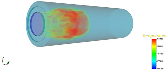
Figure 1.
Volume rendering of combustion chamber. The scalar mapping bar shows the correspondence between temperature and color.

Figure 2.
Contour line (a), texture (b), and streamline (c) visualization.
In conclusion, the majority of flow field visualization techniques only require a portion of the original data as the input data or the calculated or processed data derived from the original data for rendering images. However, volume rendering requires complete original data and the spatiotemporal overhead of the ray casting calculation is extremely high, making it challenging to support the drawing of large-scale unsteady animation with the hardware environment of conventional computers. Consequently, the current unsteady animation is typically based on geometric visualization techniques, which are created by loading and rendering the flow field’s visual surface in time steps. The actual data required consists primarily of flow field surface data consisting of 0D points, 1D lines, and 2D surfaces. To make animation visualization techniques applicable to larger-scale unsteady data, pre-processing can be performed on unsteady data and only the minimum amount of data required to draw each time step flow field is retained, thereby reducing animation visualization’s memory consumption and inter-frame delay.
3.2. Unsteady Animation Visualization Method
Figure 3 shows the overall procedure of the unstructured unsteady flow field animation visualization method. To avoid animation latency due to data I/O, this method uses a pre-processing technique that loads all unsteady data before drawing the animation in time steps. Upon loading the flow field file, the flow field variables and flow field meshes that make up the majority of the data file’s content are analyzed to simplify them based on the minimal amount of data required for animation visualization. Before loading the data centrally, the user can explore the unsteady flow field with a visualization method that renders while the data is being loaded. In this way, the user can initially explore the flow field information to identify the target variables for unsteady animation studies. After the user has performed a preliminary analysis of the flow field’s characteristics, they can set the variable loading parameters as required and begin reading all of the time-step data into memory and simplify them, thereby reducing the unsteady data size while ensuring the accuracy of the visualization results. So that it can be applied to large-scale unstructured unsteady flow fields, the simplified dataset is then used as the input data for animation visualization. Simplified data contains the flow field surface mesh and the required flow field variables for surface rendering. These data enable quick access in memory to generate the graphics’ elements and form the flow field animation. This method enables quick access to simplified data in memory, allowing for interactive animation analysis and the observation of the unsteady flow field development in any region at a higher rendering frame rate.
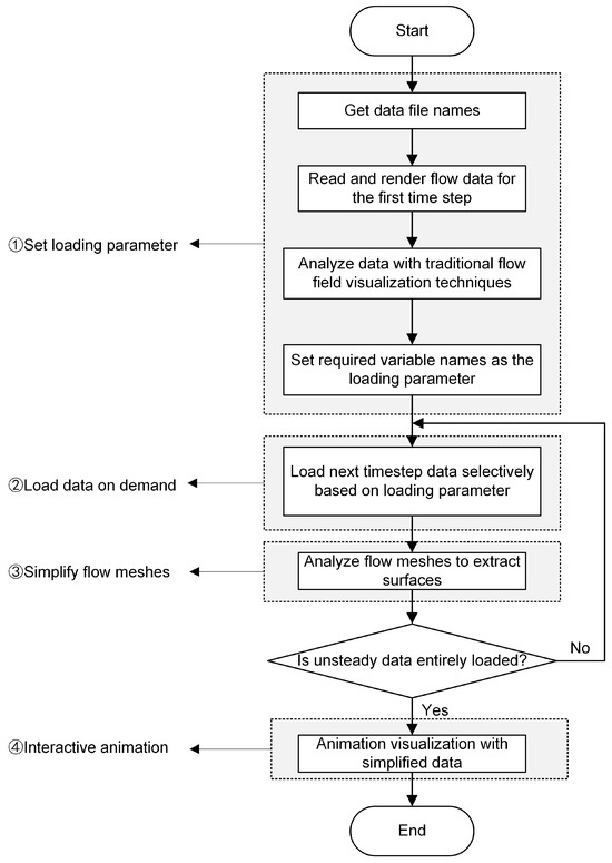
Figure 3.
Unsteady flow animation visualization process.
3.2.1. Loading Parameter
As shown in Figure 4, the I/O process of the CFD simulation data consists primarily of flow field mesh construction and flow field variable loading. Although flow field variables are used to record the physical quantities of vertices and cells, their reading process is relatively independent of the flow field mesh and these two types of data are typically loaded as separate data objects in the actual I/O process, then linked by the vertex or cell index. Since the flow field mesh has spatial connection relationships, it is necessary to obtain the complete mesh cell information to analyze and simplify it; therefore, the flow field mesh simplification cannot be conducted until the data I/O of each time step has been completed. However, there is no complex spatial relationship between flow field variables, and flow field variable simplification can be accomplished at the I/O stage by utilizing the variable description information contained within the data file.
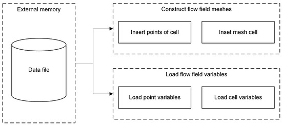
Figure 4.
Process of data loading.
Multiple flow field variables, like fluid velocity, temperature, and pressure, are frequently included in scientific simulation data. Additionally, only one or a few variables are actually required to serve as the research object when analyzing a specific, time-varying scientific problem. Therefore, the user should be given the option to select the flow field variables that best suit their needs. The principle of selective data loading is to load only the flow field variables of interest to the user and to avoid loading redundant data. By doing this, the data size reduction goal is met while the animated visualizations are kept. As depicted in Figure 5, studying the attitude change in a missile after launch can use the pressure distribution on the upper and lower surfaces of the missile (involving the pressure variable) or the airflow direction around the missile (involving the velocity variable) and other variables become redundant and can be simplified at this time. To aid users in determining the necessary flow field variables, the first timestep of the unsteady flow field is loaded in the form of a steady flow field. Data preprocessing can be performed using common visualization techniques such as isosurfaces, cloud maps, streamlines, etc. to achieve the desired visualization effect and then determine the required flow field variables. To facilitate a more thorough analysis of unsteady data when determining the necessary variables, the proposed method enables unsteady animation using the conventional loading and drawing method. In this playback mode, only the current time step flow field data is loaded into memory. Although the animation latency is high, this mode allows users to investigate the temporal characteristics of unsteady data. If users are unable to determine the required flow field variables based on the first timestep flow field alone, they can switch to any time step and confirm the animation’s required variables via a comprehensive analysis of the data from multiple time steps.
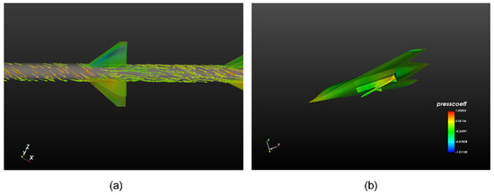
Figure 5.
Geometry−based visualization (a) plots the velocity vector arrows, and (b) displays the cloud map with pressure coefficient variable.
After obtaining the user-required flow field variables through the preceding data preprocessing, these variable names are used as reading parameters to sequentially read the data files of all time steps of the unsteady flow field. The data loading algorithm filters all data according to the reading parameters, retaining only the necessary variables and avoiding the reading of redundant variables, thereby reducing memory consumption and accelerating data I/O.
3.2.2. Selective Data Loading
After obtaining the flow field variable reading parameters, the external storage data files can be parsed sequentially and redundant variables that the user is not interested in are skipped over via selective data reading. Figure 6 shows the composition of unstructured flow field simulation data. These data have an explicitly defined topological structure. Usually, a list of points per cell is used to represent this structure. However, compared to structured data, this approach uses more storage space. Together with the geometric structure, it constitutes the flow field mesh, which is the primary component of the unstructured flow field data file. Typically, the storage of variable data consists of variable description information and variable values stored sequentially. After being read into memory, the variables are associated with the corresponding geometric vertices or mesh cells via point or cell ID numbers.
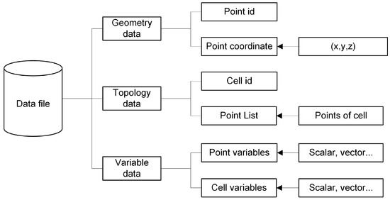
Figure 6.
Components of unstructured flow field simulation data.
Different CFD software vendors have developed various file formats for flow field data, which, according to the data storage mechanism, can be classified as single-file or multi-file storage types. For the single-file variety, each time step flow field’s information is stored in a single file. The flow field variables occupy a continuous storage space in the file, where each variable is separated into a separate data area and the area header contains the variable’s description information, such as variable name, variable distribution (on vertices or cells), variable value type, etc. In addition to storing vertex-, cell-, and variable-related data in discrete files, the multi-file type additionally includes an I/O entry file. The entry file contains the filenames of various data files, allowing the reading algorithm to locate the flow field mesh and variable data files. In combination with the data documentation supplied by the vendor, the following reading algorithm may be applied to the flow field variable data to accomplish on-demand loading of the flow field variables:
Input: flow field data file;
Output: collection of arrays of selected flow field variables.
Step one, read the variable description information: Read the variable’s description information from the file and parse the variable’s name, data type, length, and other description information. Check, for each variable, whether its name is included in the user-specified reading parameters. If yes, proceed to step two; if no, continue to step three.
Step two, load the variable data: Load the data values of each variable one by one into the variable array in memory based on the data type and length specified in the variable description information and designate the variable as a vertex or cell variable based on its distribution position. After loading the variable in question, proceed to step four.
Step three, skip redundant variables: For simulation data stored in a single file, calculate the number of bytes occupied by the variable in the binary data file based on the variable type and number and skip the current variable data area by setting the file pointer offset; for simulation data stored in separate files, directly skip the data file that contains the variable based on its name.
Step four, read the remaining variables: If there are still unprocessed flow field variables in the data file, go to step one. After processing all the variable data in the data file, save the variable arrays inserted into memory along with the variables’ names, data type, and other data as a flow field variable dataset.
3.2.3. Mesh Simplification
The flow field mesh stores the spatial information of the flow field, and because the mesh cells of the unstructured flow field data have various types and complex connection relationships, the memory overhead of importing the unstructured mesh is substantial. Since the complete cell connection relationship can only be obtained after reading all the meshes, the mesh simplification must be conducted after the single time step data I/O has been completed; it cannot be simplified like the flow field variables during the I/O stage. The flow field mesh simplification algorithm analyzes the flow field’s topology structure, obtains the surface mesh necessary for drawing each time step’s flow field, and divides it into simple linear cells to reduce the memory overhead and accelerate image rendering. To extract and divide the surface mesh, the algorithm separately processes three-dimensional and non-three-dimensional mesh cells, where non-three-dimensional cells all belong to the visible portion of the surface rendering and therefore only need to be divided into simple linear cells. The processing of three-dimensional cells is more intricate; therefore, it is necessary to first extract the outer surface of the cell as the visible portion before dividing the surface cell into simple linear surfaces for visualization input.
Non-Three-Dimensional Cells
Zero-dimensional (0D) cells consist only of vertex and multi-vertex cells, which are made up of two or more vertices with no connection between them. As shown in Figure 7, a vertex cell can be saved directly to the surface output cell, while a multi-vertex cell is divided into multiple vertex cells and then the variable attributes of the corresponding cells are copied and processed as vertex cells.
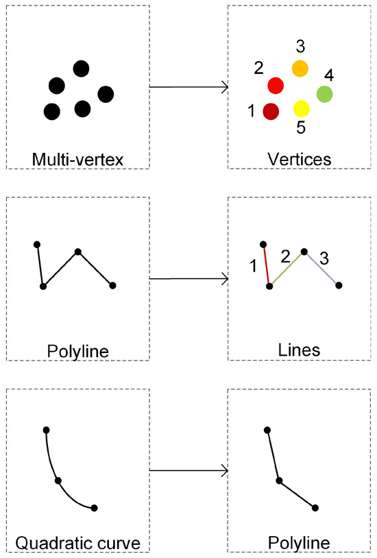
Figure 7.
Simplification method of multi-vertex, polyline, and quadratic curve. The dots in the figure represent the points of the cell. The numbers record the index of the cell after subdividing.
There are three different varieties of 1D cells: line, polyline, and quadratic curve. A polyline is a cell that consists of multiple lines. The method of processing is comparable to the 0D cell. As output cells, the polyline is divided into several separate lines during mesh simplification. A quadratic curve is the simplest nonlinear cell, defined by its beginning point, ending point, and inflection point. When rendering nonlinear cells, computer graphics libraries must typically subdivide nonlinear cells into linear cells before converting them into linear primitives for rendering. Consequently, it can be directly subdivided into linear cells when simplifying the mesh, without both affecting the final visual effect and requiring repetitive cell subdivision operations during rendering. As shown in Figure 7, a quadratic curve cell can be viewed as a polyline composed of two lines, after which a straightforward linear cell division is performed.
Two-dimensional cells consist of triangle, quadratic triangle, quadrilateral, quadratic quadrilateral, etc. Even though there are more cell types than 0D and 1D, the processing principle is still to subdivide nonlinear cells into linear cells and then divide the linear cells into simple linear cells. Using a quadratic quadrilateral cell as an example, first add a midpoint, then use the midpoint as a common vertex and form four linear quadrilateral cells with the original eight vertices, as depicted in Figure 8. This completes the simplification of a nonlinear 2D cell.
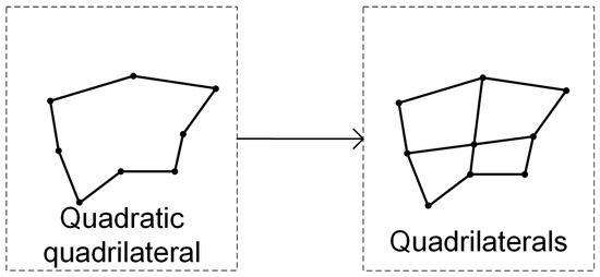
Figure 8.
Subdivision of quadratic quadrilateral.
Three-Dimensional Cells
The processing of 3D cells is the most complicated part of mesh simplification, which requires analyzing all 2D surfaces of each 3D cell and only retaining the 2D surfaces that constitute the flow field surface. The judgment rules are as follows: let the set of 3D cells in the flow field be V, the set of surfaces that constitute the flow field surface be S, and the vertices of a 2D surface f be P, then for this 2D surface, if there exists a unique such that , that is, all vertices in P are contained in the unique 3D cell v, then the surface f is the external surface of the flow field. On the contrary, if there is no such unique 3D cell, then the surface f is the internal surface of the flow field. Let the set of vertices of 3D cell v be . Then, for a 2D surface , where denotes the ith vertex of f, the judgment process can be described as follows:
For each 2D surface of a 3D cell, the connectivity of the 3D cell where it is located can be analyzed to determine whether the surface belongs to the external surface of the flow field. First, obtain all the vertices that make up the 2D surface and then traverse all the cells connected to the current cell. If there exists any adjacent cell that contains these vertices, it means that it is shared by at least two 3D cells, so it is not an external surface. Otherwise, it can be processed as an external surface of the flow field according to the 2D cell. However, this traditional method based on cell connectivity requires multiple traversals of adjacent mesh cells, and for the data with n 2D surfaces contained in 3D cells, the algorithm time complexity is as high as .
In order to reduce the time overhead of extracting the surface mesh, according to the condition described in Equation (1), it can be known that for the 2D surface that constitutes the flow field surface, it will only appear once when traversing all the 2D surfaces of the 3D cells, and the surfaces that appear repeatedly must be internal surfaces. Therefore, the unique key–value pair characteristics of the hash table can be used to efficiently deduplicate and then quickly obtain the 2D surfaces that constitute the flow field surface mesh. A structure based on a hash table was designed, as shown in Figure 9. The data subject consisted of the vertices that make up the 2D surface and the id of the 3D cell where they are located, to enable surface deduplication, random access, and sequential access for constructing the output data.
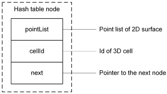
Figure 9.
Hash table node structure.
Among them, pointList is the vertex list that makes up the surface, stored in ascending order of vertex id, and cellId is the id number of the 3D cell where the surface is located. It is used to copy the variable data on the cell when creating the output cell of the surface mesh. The "next" pointer, which points to the next inserted node, is also used to handle the mapping address conflicts. The hash table uses the smallest id number in the vertex list as the key value for random access. When a conflict occurs, a chained hash table is used to store the new surface node. When inserting, the repeated surface feature is that the vertex list is exactly the same as the existing node. The repeated surface can be obtained via node random access and comparison, then cellId is set to −1 (an illegal cell id value) to mark it as an internal surface. Using this data structure, only one traversal of the 2D surfaces can obtain all the 2D surfaces that constitute the flow field surface, thereby reducing the algorithm time complexity to . After completing the traversal, cellId in each table node indicates whether the current surface is an external surface. By sequentially accessing through the next pointer, each external surface can be efficiently inserted into the flow field surface mesh output via the algorithm.
3.2.4. Interactive Animation
After performing selective reading and simplification processing on the unsteady dataset, all the data required for animation drawing are loaded into memory and the redundant portion of the original data is removed, which significantly reduces the data size of the unstructured unsteady flow field, allowing personal computers to fully load the simplified dataset, thereby eliminating the animation delay caused by data I/O and accelerating image rendering. Based on the VTK 8.2 (Visualization Toolkit), interactive animation visualization for large-scale unstructured unsteady flow fields is implemented using data simplification algorithms.
The data processing and animation visualization proposed in this paper are implemented based on VTK. The animation is made responsive to the real-time interaction during playback by using the event observing mechanism of VTK to add a timer event to the VTK interactor. This ensures that the visualization input data is updated according to the time interval specified by the user. The timer is used to create animation updates and interactions within an animation. The VTK interactor offers a few fundamental interactivity features. Whenever the user conducts interactions such as viewpoint translation, zooming, rotation, etc., the timer event response will be temporarily paused and resumed once the interaction is complete. The animation enables examination of the time-varying characteristics of the unsteady flow field and interaction with the animation to analyze the spatial distribution of the specific time-step flow field.
As shown in Figure 10, besides the conventional interaction methods, a time-step interaction widget was designed to support the control of animation playback. This widget offers more interactive animation control options than the one provided by ParaView 5.10. It allows the application of the proposed animation visualization methods, in addition to traditional player controls such as play, pause, and toggle timestep operations. The animation by default uses the playback mode of drawing while reading data, similar to ParaView. The mode of centralized data loading and playback can be chosen by clicking on the “Load animation” button. This enables the use of one or all selective I/O and mesh simplification preprocessing to increase the animation frame rates. The “Data type” drop-down box allows easy switching between the raw data and the simplified data. Moreover, the parameters of the VTK timer are exposed to the user so that the animation playback speed can be manually adjusted by modifying its trigger interval. The rendering window and timestep widget facilitate easy interaction for better use of the animation visualization.
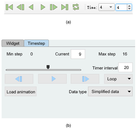
Figure 10.
Animation timestep interaction widget (a) shows the timestep widget in ParaView, and (b) shows our timestep widget, which has a more user-friendly interface and supports more animation configurations.
4. Experiment
The experiment utilizes four groups of unstructured unsteady datasets and the data processing method proposed in this paper to perform animation visualization. The following describes the computer hardware configuration used in the experiment: Intel Xeon (Skylake) processor with 8 cores at 3.00 GHz, 32 GB of DIMM memory (16 GB × 2) and an Nvidia GRID P40-1Q graphics card with 1 GB of video memory. Table 1 contains four datasets derived from simulations of time-varying phenomena. Variable selective loading, mesh simplification, and memory optimization combining the two methods were carried out on the experimental datasets to confirm the generalizability of the method proposed in this paper. Among them, dataset 1’s flow field mesh contains only 2D cells and the data memory ratio for flow field variables is relatively high. Dataset 2 is a single-variable flow field composed of 3D cells; therefore, the method for selectively loading variables cannot be applied. Both dataset 3 and dataset 4 are large-scale, unsteady flow field data consisting of 2D and 3D cells and multiple variables that cannot be imported directly and entirely into memory for animation visualization.

Table 1.
Information on experimental data.
4.1. Variable Simplification
Typically, CFD simulation simulates and solves the Navier–Stokes equations using conservation laws such as mass and momentum conservation. The equation contains multiple variables such as fluid velocity, pressure, density, temperature, etc., and velocity is the most significant unknown among them, as it directly affects the fluid’s momentum and energy and can reveal the fluid’s motion state and motion characteristics, which are the primary research topics. Therefore, in the experiment of variable loading on demand, velocity is chosen as the visualization-loading variable, while other variables are regarded as redundant data and omitted loading. The experimental outcomes are presented in Table 2. According to the experimental results of dataset 1, dataset 3, and dataset 4, loading the flow field variables on demand has a certain optimization effect when there are more categories of variables in the dataset. The optimization effect of dataset 1 with a simple topology structure and a high proportion of variable data is more apparent. The memory ratio indicates the memory ratio of loading all the data with the selective I/O method compared to using the VTK file reader directly. The selective I/O method only loads the velocity variable in the data file and saves the extra space by not storing irrelevant variables.

Table 2.
Experimental results of load-on-demand variable-optimized memory.
Dataset 3 and dataset 4 reduce the memory overhead by 2 GB compared to the original data, but cannot load all the time steps into memory to eliminate the playback delay caused by inter-frame data I/O; dataset 2 is simulation data with a single flow field variable, so variable simplification is not possible. Experimental findings indicate that variable simplification has an optimization effect on multivariable flow fields. However, the majority of the memory burden associated with loading unstructured data is due to its complex topology structure. To further reduce the size of unsteady data, it is essential to combine the flow field mesh simplification method.
4.2. Mesh Simplification
Structured simulation data can use its arrangement principles to store the flow field mesh implicitly, whereas unstructured data requires extra space to record complex, unordered, and diverse mesh cells and cell connectivity. The mesh simplification algorithm analyzes the flow field topology structure based on the surface mesh required for surface drawing and then replaces the original data with the minimum data required for visualization input, attaining the goal of reducing the data size. Table 3 displays the outcomes of applying the mesh simplification method and combining it with the technique described in Section 3.1 in order to optimize the memory of experimental datasets. The topology structures of dataset 2, dataset 3, and dataset 4 are primarily composed of 3D cells and the memory requirements are drastically reduced after surface extraction and linear surface division. The mesh simplification method has a greater effect when the proportion of 3D cells in the dataset is considerable, as indicated by the data in Table 4. Data preprocessing leads to a significant memory reduction even in dataset 1, which does not contain 3D cells. The combined optimization method makes use of both selective loading and mesh simplification. By employing this method, high memory reductions were achieved for all experimental datasets. It indicates that the method is highly universal for unstructured unsteady data with various composition structures. A personal computer can display larger-scale unsteady flow fields in animated form as a result of data simplification and centralized loading of the entire time step. The data processing methods are based on the VTK rendering pipeline, which also applies to the VTK-based ParaView. A new playback mode can be created by substituting the data read after data I/O with the simplified data at each time step.

Table 3.
Mesh simplification and combinatorial optimization memory experiment results.

Table 4.
Average time cost of the flow field surface mesh exraction algorithm.
The outer surface extraction algorithm for 3D cells on unstructured meshes was analyzed and improved. The conventional VTK surface extraction algorithm uses cell intersection to determine whether a 2D surface is an external surface. This requires first querying which cells contain vertices within a 2D surface. The list of points that make up these cells is then intersected. It can only be referred to as an external surface if these points do not appear repeatedly in any cell. VTK reduces the overhead of seeking out cells by constructing a table of connected relations for unstructured mesh cells. However, the time it takes to build a table of connections is also costly. A hash structure was constructed to assist the lookup surfaces and reduce the number of lookups and the time cost of unsteady data processing for surface deduplication. It can significantly decrease the amount of time needed for data preprocessing, which will improve user experience.
Table 4 shows the time overhead of the proposed method compared to common surface extraction techniques. Dataset 1 was not tested because it had no 3D cells. The experimental results indicate that the proposed method can achieve more than twice the efficiency of the existing algorithm on dataset 2, dataset 3, and dataset 4, which mainly consist of 3D cells, thus significantly reducing the data processing time. However, the algorithm’s efficiency decreases gradually for complex and large-scale mesh structures due to the overhead of managing insertion conflicts in the hash structure.
4.3. Animation Playback Delay
Table 5 records the average inter-frame delay of the experimental data animation playback using three different methods. Method (1) takes the raw flow field data as the input data. At each time step, it performs the data loading and image rendering processes. Consequently, most of the delay in method (1) results from data I/O. ParaView 5.10 currently employs this technique. All the time-step data is read into memory via Method (2). The flow field data is acquired directly to render the animation. This method cannot be applied when the data exceeds the memory capacity. Method (3) expands on Method (2) by using data simplification to reduce the amount of data. Only a smaller portion of the data required for visualization will be loaded into memory using selective loading and mesh simplification. Mesh simplification contributes significantly to the decrease in animation latency and variable loading has little effect on visualization calculations.

Table 5.
Average interframe delay for animation playback.
Among the datasets, dataset 3 and dataset 4 are too large in scale, and method (2) cannot directly load all the time steps into memory, so the first 20 time steps are used for research. To reduce the impact of random factors, the experiment records the total time spent playing the dataset animation multiple times and calculates the average inter-frame delay by dividing it by the total number of time steps. Compared with method (1), method (2) eliminates the inter-frame data I/O time overhead. But, when the data scale is larger (dataset 2, dataset 3, and dataset 4), the rendering and drawing time of each time step flow field increases significantly, which causes a decrease in the smoothness and real-time interactivity of the animation. Method (3) uses the simplified unsteady data as the visualization input, which can reduce the graphics’ rendering computation based on eliminating the inter-frame I/O time overhead, thereby further reducing the animation playback delay. As can be seen from Table 5, the simplified experimental dataset was used as the visual input via the proposed method, which achieved an average inter-frame delay of animation rendering less than 100 ms. This enabled real-time response to the user’s visual interaction.
The data simplification improved the animations’ frame rates but also affected the visualizations. The selective reading of variables had minimal impact, as the required variables were usually known. Other variables could be quickly read using the file’s variable description information. However, the mesh simplification, which retained only the externally visible part of the flow field, altered some of the visualization results. Figure 11 illustrates the results of cloud map coloring with velocity at the sixth time step of dataset 2. They had slightly different color mappings because of the internally invisible points and cells and the variables distributed over them, which were removed. Thus, the range of values of the variables differed. The velocity in Figure 11a has a maximum value of 1.5183, whereas the maximum velocity in Figure 11b is 1.475. Interactions requiring inner data from the flow field, such as isosurface extraction, may produce different results. The complete isosurface of the turbulent region Figure 11c can be extracted from the flow field of Figure 11a. Only contour lines can be extracted for the data in Figure 11b with the same settings. Nonetheless, it offered an overall overview of the unsteady flow field and the visible part of the mesh was unchanged. The proposed unsteady animation visualization method enabled a global overview of the unsteady flow field using simplified data. Raw data could be used for a more comprehensive visual analysis when needed.
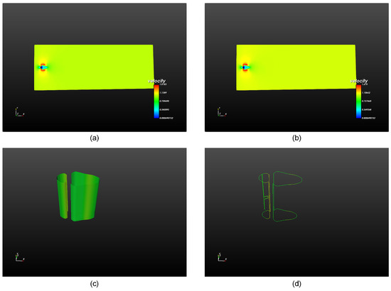
Figure 11.
Comparison of dataset 2 visualization (a) is based on original data; (b) is based on simplified data; (c) is an isosurface extracted from (a); and (d) is an isosurface extracted from (b).
5. Conclusions and Future Work
This paper examines the current techniques for animating unsteady flow fields. Personal computers face resource constraints to animate large-scale unstructured flow fields. Unsteady data compression methods using hierarchical structures and differential coding are efficient but not suitable for unstructured flow fields. Compressing unstructured flow field data with time and space dimensions requires designing fast decompression or customized visualization algorithms, which is difficult. This paper presents two data simplification algorithms using ParaView’s animation method. The algorithms simplify the flow field data using variables and meshes, which are the main components, and enable direct memory reading of the simplified data. The two data simplification algorithms in this paper can lower the memory cost of complex datasets by over 90%, as shown by four experiments. On this basis, personal computers can load simplified data directly into memory, thus avoiding inter-frame delays caused by data I/O. By comparing the three playback methods, it is demonstrated that the method in this paper can visualize the animation of large-scale unstructured unsteady flow fields on a personal computer and can respond to user interactions within 100ms in real time. The method in this paper can enhance the user’s analysis of unsteady flow fields, unlike the original playback method in ParaView. The method does not use data compression techniques, so the simplified data can be rendered directly by using existing flow field visualization techniques, which is very versatile.
However, the animations are rendered using geometry-based flow field visualization techniques, so the simplified data lacks information about the interior of the flow field. The simplified data cannot be used directly for volume rendering or isosurface extraction. The user can switch between the simplified and raw data anytime with the timestep widget in this paper. This enables the analysis of the unsteady flow field with other visualization methods, combining the benefits of the two playback methods. Feature tracking and animation visualization will be used in future work to extract and analyze the internal regions and time-varying features of large-scale unsteady flow fields. Thread parallelism rendering techniques will also be explored to leverage the multi-core performance of PCs and enhance the animation frame rate.
Author Contributions
Methodology, X.T. and Y.H.; Writing—review and editing, C.Y.; Visualization, C.Y.; Writing—original draft, X.T. and Z.H.; Software, Z.H. and Y.H.; Supervision, Y.W.; Validation, Y.H.; Project administration, Y.W.; Funding acquisition, Y.W. All authors have read and agreed to the published version of the manuscript.
Funding
This work was supported in part by the National Numerical Windtunnel Project (NNW2019ZT6-A17) and the National Defense Basic Research Project (JCKY2022404C001).
Institutional Review Board Statement
Not applicable.
Informed Consent Statement
Not applicable.
Data Availability Statement
Publicly available datasets were analyzed in this study. This data can be found here: [https://nnw-vvdb.nssdc.ac.cn:8443/VVDB/doSSOLoginNew.rdm]
Conflicts of Interest
The authors declare no conflict of interest.
References
- Xu, L.; Jiang, T.; Wang, C.; Ji, D.; Shi, W.; Xu, B.; Lu, W. Experiment and Numerical Simulation on Hydraulic Loss and Flow Pattern of Low Hump Outlet Conduit with Different Inlet Water Rotation Speeds. Energies 2022, 15, 5371. [Google Scholar] [CrossRef]
- Liu, L.; Silver, D.; Bemis, K. Visualizing events in time-varying scientific data. J. Vis. 2020, 23, 353–368. [Google Scholar] [CrossRef]
- Le, T.L.; Vuong, T.H.N.; Phung, T.H. Numerical Computation of Hydrodynamic Characteristics of an Automated Hand-Washing System. Computation 2023, 11, 167. [Google Scholar] [CrossRef]
- Kniss, J.; McCormick, P.; McPherson, A.; Ahrens, J.; Painter, J.; Keahey, A.; Hansen, C. Interactive texture-based volume rendering for large data sets. IEEE Comput. Graph. Appl. 2001, 21, 52–61. [Google Scholar] [CrossRef]
- Bai, Z.; Tao, Y.; Lin, H. Time-varying volume visualization: A survey. J. Vis. 2020, 23, 745–761. [Google Scholar] [CrossRef]
- Ma, K.L.; Camp, D.M. High performance visualization of time-varying volume data over a wide-area network. In Proceedings of the SC’00: 2000 ACM/IEEE Conference on Supercomputing, Dallas, TX, USA, 4–10 November 2000; p. 29. [Google Scholar]
- Shen, H.W.; Chiang, L.J.; Ma, K.L. A fast volume rendering algorithm for time-varying fields using a time-space partitioning (TSP) tree. In Proceedings of the Visualization ’99 (Cat. No.99CB37067), San Francisco, CA, USA, 24–29 October 1999; pp. 371–545. [Google Scholar]
- Du, Z.; Chiang, Y.J.; Shen, H.W. Out-of-core volume rendering for time-varying fields using a space-partitioning time (SPT) tree. In Proceedings of the 2009 IEEE Pacific Visualization Symposium, Beijing, China, 20–23 April 2009; pp. 73–80. [Google Scholar]
- Ma, K.L.; Shen, H.W. Compression and Accelerated Rendering of Time-Varying Volume Data. 2000. Available online: https://escholarship.org/uc/item/26w9886k (accessed on 17 September 2023).
- Wang, C.; Gao, J.; Li, L.; Shen, H.W. A multiresolution volume rendering framework for large-scale time-varying data visualization. In Proceedings of the Fourth International Workshop on Volume Graphics, Stony Brook, NY, USA, 20–21 June 2005; pp. 11–223. [Google Scholar]
- Hansen, C.D.; Johnson, C.R. Visualization Handbook; Butterworth-Heinemann: Burlington, MA, USA, 2005; pp. 511–530. [Google Scholar]
- Ibarria, L.; Lindstrom, P.; Rossignac, J.; Szymczak, A. Out-of-core compression and decompression of large n-dimensional scalar fields. Comput. Graph. Forum 2003, 22, 343–348. [Google Scholar] [CrossRef]
- Linsen, L.; Pascucci, V.; Duchaineau, M.A.; Hamann, B.; Joy, K.I. Hierarchical representation of time-varying volume data with/sup 4//spl radic/2 subdivision and quadrilinear B-spline wavelets. In Proceedings of the 10th Pacific Conference on Computer Graphics and Applications, Beijing, China, 9–11 October 2002; pp. 346–355. [Google Scholar]
- Wilhelms, J.; Van Gelder, A. Multi-dimensional trees for controlled volume rendering and compression. In Proceedings of the 1994 Symposium on Volume Visualization, Washington, DC, USA, 17–18 October 1994; pp. 27–34. [Google Scholar]
- Silva, C.T.; Comba, J.L.D.; Callahan, S.P.; Bernardon, F.F. A survey of GPU-based volume rendering of unstructured grids. Revista Informática Teórica Apl. 2005, 12, 9–29. [Google Scholar]
- Guthe, S.; Straßer, W. Real-time decompression and visualization of animated volume data. In Proceedings of the Visualization, 2001, VIS’01, San Diego, CA, USA, 21–26 October 2001; pp. 349–572. [Google Scholar]
- Mensmann, J.; Ropinski, T.; Hinrichs, K. A GPU-supported lossless compression scheme for rendering time-varying volume data. In Proceedings of the 8th IEEE/EG International Conference on Volume Graphics, Norrköping, Sweden, 2–3 May 2010; pp. 109–116. [Google Scholar]
- Chiueh, T.C.; Ma, K.L. A parallel pipelined renderer for time-varying volume data. In Proceedings of the 1997 International Symposium on Parallel Architectures, Algorithms and Networks (I-SPAN’97), Taipei, Taiwan, 20 December 1997; pp. 9–15. [Google Scholar]
- Yu, H.; Ma, K.L.; Welling, J. A parallel visualization pipeline for terascale earthquake simulations. In Proceedings of the SC’04: 2004 ACM/IEEE Conference on Supercomputing, Pittsburgh, PA, USA, 6–12 November 2004; p. 49. [Google Scholar]
- Wang, R.X.; Wang, R.; Fu, P.; Zhang, J.M. Portable interactive visualization of large-scale simulations in geotechnical engineering using Unity3D. Adv. Eng. Softw. 2020, 148, 102838. [Google Scholar] [CrossRef]
- Bernardon, F.F.; Callahan, S.P.; Comba, J.L.; Silva, C.T. An adaptive framework for visualizing unstructured grids with time-varying scalar fields. Parallel Comput. 2007, 33, 391–405. [Google Scholar] [CrossRef]
- Li, S.; Cai, X.; Wang, W.; Wang, P.; Wang, H.; Shen, E. Large-Scale Flow Field Scientific Visualization; National Defense Industry Press: Arlington, VA, USA, 2013; pp. 20–25. [Google Scholar]
- Munkberg, J.; Chen, W.; Hasselgren, J.; Evans, A.; Shen, T.; Müller, T.; Gao, J.; Fidler, S. Extracting Triangular 3D Models, Materials, and Lighting From Images. In Proceedings of the 2022 IEEE/CVF Conference on Computer Vision and Pattern Recognition (CVPR), New Orleans, LA, USA, 18–24 June 2022; pp. 8270–8280. [Google Scholar]
- Max, N. Optical models for direct volume rendering. IEEE Trans. Vis. Comput. Graph. 1995, 1, 99–108. [Google Scholar] [CrossRef]
- Fan, L.; Chen, C.; Zhao, S.; Zhang, X.; Wu, Y.; Wang, F. Multi-threaded parallel projection tetrahedral algorithm for unstructured volume rendering. J. Vis. 2021, 24, 261–274. [Google Scholar] [CrossRef]
- Laramee, R.S.; Erlebacher, G.; Garth, C.; Schafhitzel, T.; Theisel, H.; Tricoche, X.; Weinkauf, T.; Weiskopf, D. Applications of texture-based flow visualization. Eng. Appl. Comput. Fluid Mech. 2008, 2, 264–274. [Google Scholar] [CrossRef][Green Version]
- Vinuesa, R.; Lehmkuhl, O.; Lozano-Durán, A.; Rabault, J. Flow Control in Wings and Discovery of Novel Approaches via Deep Reinforcement Learning. Fluids 2022, 7, 62. [Google Scholar] [CrossRef]
- Guillou, P.; Vidal, J.; Tierny, J. Discrete Morse Sandwich: Fast Computation of Persistence Diagrams for Scalar Data—An Algorithm and A Benchmark. IEEE Trans. Vis. Comput. Graph. 2023; preprint. [Google Scholar] [CrossRef] [PubMed]
Disclaimer/Publisher’s Note: The statements, opinions and data contained in all publications are solely those of the individual author(s) and contributor(s) and not of MDPI and/or the editor(s). MDPI and/or the editor(s) disclaim responsibility for any injury to people or property resulting from any ideas, methods, instructions or products referred to in the content. |
© 2023 by the authors. Licensee MDPI, Basel, Switzerland. This article is an open access article distributed under the terms and conditions of the Creative Commons Attribution (CC BY) license (https://creativecommons.org/licenses/by/4.0/).