Gaussian Mixture Model for Marine Reverberations

Abstract

Ocean reverberations, a significant interference source in active sonar, arise as a response generated by random scattering at the receiving end, a consequence of randomly distributed clutter or irregular interfaces. Statistical analysis of reverberation data has revealed a predominant adherence to the Rayleigh distribution, signifying its departure from specific distribution forms like the Gaussian distribution. This study introduces the Gaussian mixture model, capable of simulating random variables conforming to a wide array of distributions through the integration of an adequate number of components. Leveraging the unique statistical attributes of reverberation, we initiate the Gaussian mixture model’s parameters via the frequency histogram of the reverberation data. Subsequently, model parameters are estimated using the expectation–maximization (EM) algorithm and the most suitable statistical model is selected based on robust model selection criteria. Through a comprehensive evaluation that encompasses both simulated and observed data, our results underscore the Gaussian mixture model’s effectiveness in accurately characterizing the distribution of reverberation data, yielding a mean squared error of less than 4‰.

1. Introduction

Active sonar systems employ transducers to emit specific waveform acoustic signals. Typical sonar signal frequencies are categorized as low (1 kHz–10 kHz), medium (10 kHz–50 kHz), and high frequencies (50 kHz–several hundred kHz), with each tailored to distinct applications. Waveforms, including pulsed waveforms, continuous waves, and frequency–modulated continuous waves, are selected to match the specific use case. Signal duration is adapted to application requirements, utilizing short pulses for target detection and longer signals for imaging or communication. The depth of signal penetration and range distance are contingent upon the interaction between frequency, water properties, and signal strength. Low frequencies penetrate deeply but have a limited range, whereas high frequencies offer an extended range with reduced penetration. Upon detecting a target, these systems generate echo signals at specific angles, which are subsequently received by hydrophones. These echo signals are frequently intertwined with a significant amount of ambient ocean noise and reverberation. Unlike ambient ocean noise, reverberation constitutes a distinctive physical phenomenon induced by the signals emitted by active sonar. It grows increasingly intricate with amplified signal strength and the multiplication of scattering elements, particularly in shallow water environments where multiple scattering effects are pronounced. Consequently, the processing of reverberation signals presents greater complexity, posing formidable challenges to active sonar technologies encompassing target detection, localization, and identification, among other functions [1,2].

From a statistical perspective, reverberation can be viewed as a non–stationary stochastic process, essentially stemming from the stochastic scattering response at the receiving end generated by randomly distributed scatterers or randomly irregular interfaces. The statistical model for reverberation was initially proposed by Faure [3], and subsequently, B. Olishevski and Middleton conducted further research on the reverberation model, referring to this theory as the FOA (First Order Ambisonics) reverberation theory model [4,5]. To address the challenge of parameter estimation in the presence of missing data, Arthur Dempster and colleagues introduced the expectation–maximization (EM) algorithm, which significantly reduces computational complexity by transforming the maximization of the likelihood function into an optimization problem involving expected values and maximization [6]. Wei HK improved the Greedy EM algorithm in the context of image processing and successfully applied it to the one–dimensional Gaussian mixture model (GMM) modeling of underwater reverberation [7]. Furthermore, the GMM is frequently employed in various domains such as cluster analysis, acoustic modeling, image segmentation, and feature extraction. Wang PB effectively modeled ocean reverberation data using a Symmetric Alpha–Stable (SαS) distribution model that adheres to a zero–mean, unimodal bell–shaped distribution [8]. Liu WS intuitively demonstrated the performance differences between traditional algorithms and the Greedy EM algorithm through numerical simulation examples [9]. To mitigate the issue of the clustering effect of the EM algorithm relying too heavily on the initial probability density center, Liu M proposed an improved EM algorithm based on the Fuzzy C–means algorithm for parameter initialization, which exhibits superior performance [10]. Fatma Najar employed the GMM, Generalized Gaussian Mixture Models (GGMMs), Bounded Gaussian Mixture Models (BGMMs), and Bounded Generalized Gaussian Mixture Models (BGGMMs) for multidimensional data clustering and assessed the robustness of the models [11]. Wen H introduced asymmetric Gaussian mixture models into finite mixture models to simulate more complex asymmetric distributions [12]. Mateusz Przyborowski presented an approximate method for the parameter learning of Gaussian mixture models in large datasets using the EM algorithm [13].

From Figure 1, it is evident that the reverberation data exhibit characteristics such as approximate zero mean, roughly equal positive and negative sample sizes, and nearly symmetrical upper and lower envelopes. Various distribution models, including Gaussian distribution, Gaussian mixture distribution, and SαS distribution, can be utilized for fitting and modeling. Despite Gaussian mixture distribution having more parameters than Gaussian and SαS distributions, it is capable of statistically modeling non–Gaussian data with non–zero mean and multiple bell shapes. Therefore, the GMM exhibits broader applicability, particularly in the context of reverberation data. Drawing from the fundamental theory of reverberation and statistical distribution characteristics, this paper initializes the parameters of GMM models corresponding to reverberation data. It employs the EM algorithm to iteratively generate models for different cluster numbers. Building upon various evaluation criteria, a statistical modeling approach for reverberation based on the Gaussian reverberation model is proposed. This method offers valuable support for investigating the characteristics of ocean reverberation information and advancing active sonar technology.

Figure 1. A typical waveform of element–level received data from an active sonar.

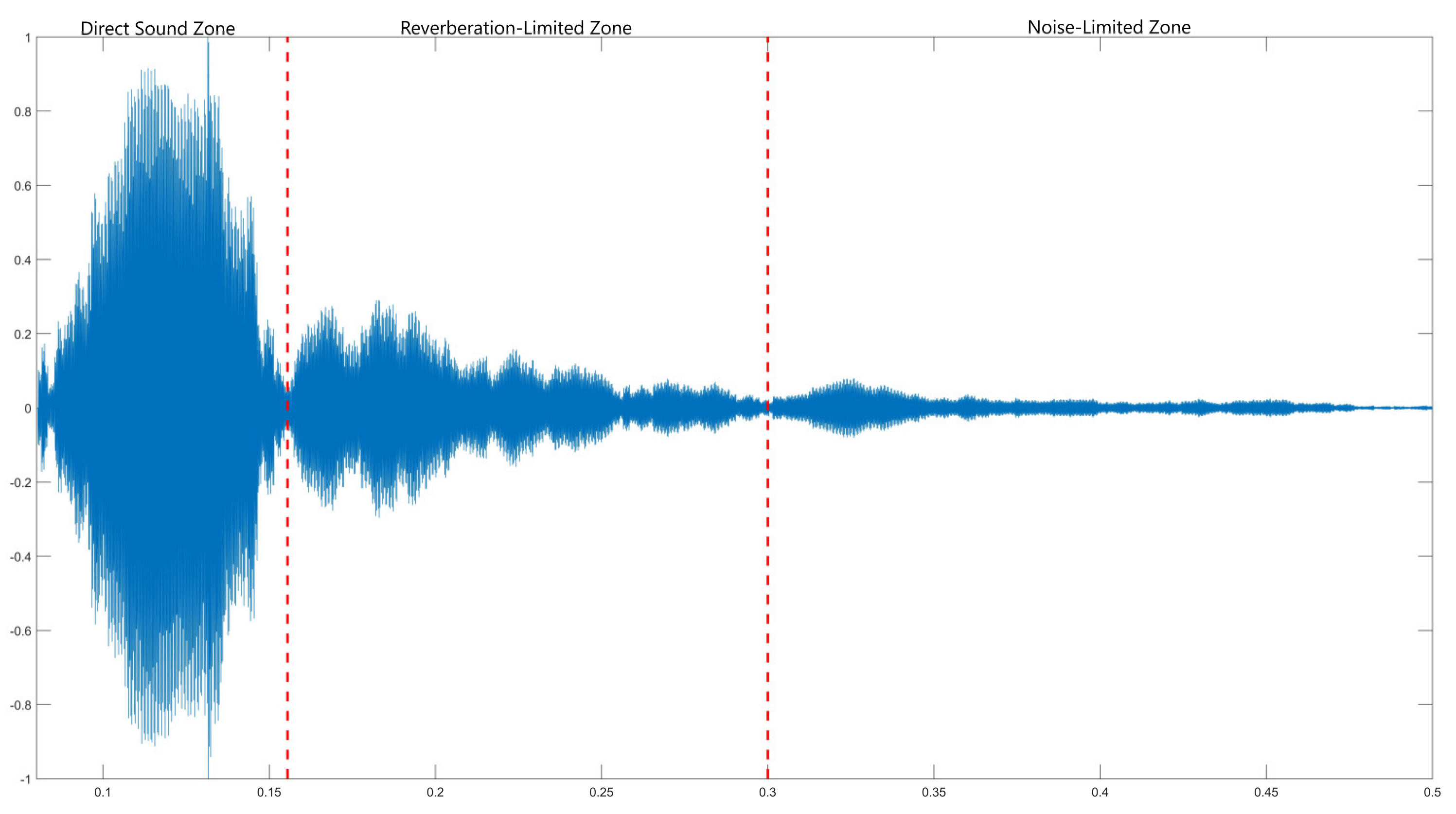
2. Theoretical and Statistical Distribution Characteristics of Reverberation

In shallow–water environments, the presence of non–uniformities in the ocean’s surface and seafloor, coupled with the abundance of scattering objects, results in the non–continuity of the physical properties of the oceanic medium. When sound waves traverse these non–uniform regions during underwater propagation, they undergo partial reflection, generating scattering. The cumulative scattering stemming from all scattering objects is termed “reverberation”. Ocean reverberation encompasses three distinct components: surface reverberation, seabed reverberation, and volume reverberation, with the first two collectively referred to as “interface reverberation” [14,15]. Despite reverberation arising from the amalgamation of echoes produced by a substantial number of chaotic scattering objects, these echoes originate from the same excitation source, endowing reverberation data with unique statistical characteristics. Middleton’s reverberation statistical model simplifies the representation of sound scattering non–uniformity in the ocean. It conceptualizes scattering objects as embedded within the seafloor or floating on the sea surface and within the seawater [16]. This model assumes their independence from one another while disregarding secondary and higher–order scattering effects [17,18].

Assuming the transducer emits a pulse signal represented by $s(t)$, the sound pressure due to reverberation at time $‘t’$ can be expressed as follows [18]:

$$p\left(t\right)=\sum _{n=1}^{N}g(r_n)f(r_n)\left|{\alpha }_n\parallel s_0\left(t-t_n\right)\right|\cdot e^{j\left[{\omega }_0\left(t-t_n\right)+{\psi }_n\left(t-t_n\right)+{\varphi }_n\right]},$$

(1)

where $g(r_n)$ denotes the count of scattering objects within the spatial microelement $∆v_n$ situated at position $r_n$. The term $f(r_n)$ signifies the round–trip propagation attenuation factor for the scattering echoes originating from the scattering objects within $∆v_n$, while $t_n$ corresponds to the arrival time of the echo. The parameter $N$ represents the overall count of scattering spatial microelements that contribute to time $t$. Let

$$\mathrm{Re}\left[p\left(t\right)\right]=x\left(t\right)\cos {\omega }_{0}t-y\left(t\right)\sin {\omega }_{0}t.$$

(2)

For the surface reverberation $p_s(t)$, as $x_s\left(t\right)$ and $y_s(t)$ follow zero–mean Gaussian distributions, the amplitude $r_s\left(t\right)={\left[x_s^2\left(t\right)+y_s^2(t)\right]}^{1/2}$ of the reverberation also follows a Rayleigh distribution [18], with probability density being as follows:

$$p\left(r\right)=\frac{r_s\left(t\right)}{{\sigma }_s^2\left(t\right)}\mathit{exp}\left[-\frac{r_s^2\left(t\right)}{{\sigma }_s^2\left(t\right)}\right],$$

where ${\sigma }_s^2(t)=E\left[x_s^2(t)\right]=E\left[y_s^2(t)\right]$, representing the average intensity of the reverberation. Similarly, it can be deduced that the amplitude of the volume reverberation $p_v(t)$ also follows a Rayleigh distribution [18].

For the seabed reverberation, as the scattering objects are fixed, the reverberation sound pressure is a periodic signal [18]:

$$p_b\left(t\right)=r_b\left(t\right){\mathrm{e}}^{f\left[{\omega }_{0}t+{\varphi }_0\left(t\right)\right]}.$$

The total reverberation is as follows:

$$p_c(t)=p_s(t)+p_v(t)+p_b(t),$$

the amplitude $r_c(t)$ of $p_c(t)$ follows a modified Rayleigh distribution, also known as the Rice distribution:

$$p(r)=\frac{r(t)}{{\sigma }_c^2(t)}\exp \left|-\frac{r^2(t)+{r_b}^2(t)}{2{\sigma }_j^2(t)}\right|I_0\left|\frac{r(t)+r_b(t)}{{\sigma }_j^2(t)}\right|,$$

(3)

where ${\sigma }_j^2\left(t\right)={\sigma }_s^2\left(t\right)+{\sigma }_v^2\left(t\right)$, and $I_0$ is the zero–order modified Bessel function [18].

The above analysis shows that reverberation is not a stationary random process. Its intensity decays rapidly over time. At each fixed time $t$, the amplitude of the reverberation follows a Rice distribution. If the seabed reverberation is neglected, then the amplitude of the reverberation follows a Rayleigh distribution. Statistical modeling can be used to describe the reverberation data. Currently, typical distributions used for this purpose include Gaussian distribution, SαS distribution, and Gaussian mixture distribution, all of which can describe data with similar statistical characteristics using their probability density function (PDF) [19].

3. Statistical Modeling of Ocean Reverberation Data Based on the Gaussian Mixture Model (GMM) Method

3.1. Gaussian Mixture Model (GMM) and Its Parameter Estimation Method (EM Algorithm)

The Gaussian mixture model is a linear combination of multiple Gaussian distributions with the following probability distribution model:

$$f\left(x;\lambda ,\mu ,\sigma \right)=\sum _{k=1}^K{\lambda }_k{p}_k(x;{\mu }_k,{\sigma }_k^2)=\sum _{k=1}^K\left\{-\frac{{\lambda }_k}{\sqrt{2\pi {\sigma }_k^2}}\mathit{exp}\left[-\frac{{(x-{\mu }_k)}^2}{2{\sigma }_k^2}\right]\right\},$$

(4)

where $K$ is the number of individual Gaussian models in the mixture model, also known as the cluster number or model order. ${\lambda }_k$ represents the mixture weight, satisfying $0<{\lambda }_k<1$ and ${\displaystyle {\sum }_{k=1}^K}{\lambda }_k=1$. When $\lambda =1$, the model degenerates into a Gaussian model. $p_k$ represents the $k-th$ Gaussian component, while ${\mu }_k$ and ${\sigma }_k^2$ represent the mean and variance of the distribution, respectively. In theory, if the number of Gaussian models fused by a certain Gaussian mixture model is large enough, and the weights set between them are reasonable enough, the Gaussian mixture model can fit any distribution [20].

The EM algorithm is used for parameter estimates in the Gaussian mixture model with latent variables. Assuming that the observed dataset is $X=\left\{x_1,x_2,\dots {,x}_N\right\}$, each data point $x_i$ is independent, and the latent parameters are $Z=\left\{z_1,z_2,\dots {,z}_N\right\}$, where $z_i$ indicates the probability that the sampling point $x_{\mathrm{i}}$ comes from a certain Gaussian distribution. Given the initial parameter value ${\mathrm{\Theta }}^{(0)}=\left\{{\lambda }_k,{\mu }_k,{\mathsf{\sigma }}_k\right\}$, the iterative solution for maximizing the likelihood function of $X$ is employed to determine the parameters $\Theta$ that optimize this likelihood function.

3.2. Improved EM Parameter Estimation Method

In the context of parameter estimation using the EM algorithm, it is crucial to predefine the number of clusters ($K$), means, and variances. Without proper initialization of these parameters, the EM algorithm is susceptible to converging towards local optima or even experiencing convergence failures [21]. In this study, we adopt a systematic approach to address this issue. Initially, we initialize the number of clusters, means, and variances by leveraging the frequency histogram of the reverberation data. Subsequently, we employ the EM algorithm for iterative parameter estimation, covering various cluster numbers. Ultimately, the selection of the most suitable model is based on rigorous evaluation metrics. The detailed algorithmic workflow is visually presented in Figure 2.

Figure 2. Statistical modeling method for ocean reverberation data based on GMM.

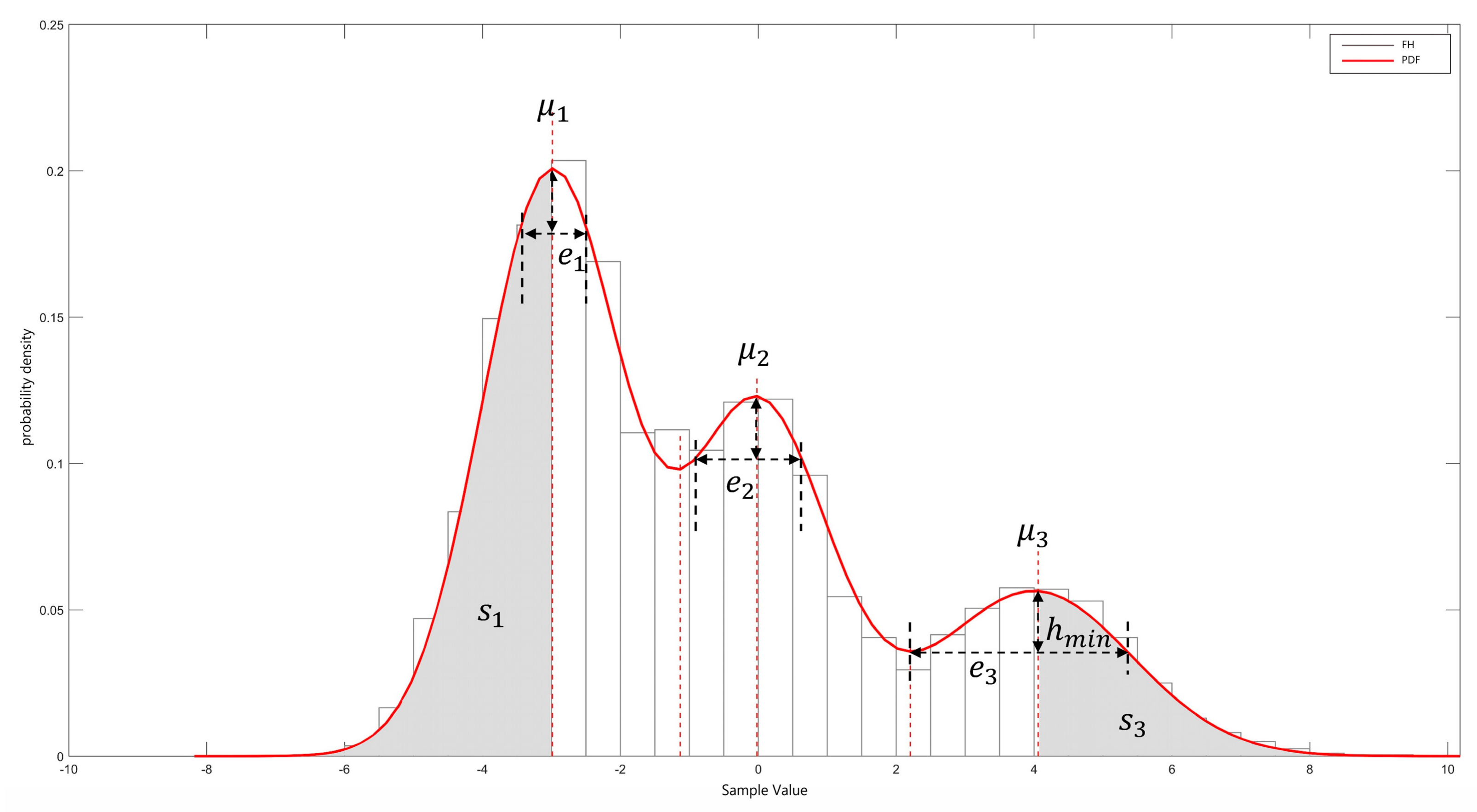
3.2.1. Parameter Initialization Based on Reverberation Data

With an ample sample size, the histogram outcomes can be deemed representative of the actual distribution. The steps for initializing data using the frequency histogram (FH) are outlined as follows:

(1) Assuming that $K_B$ represents the optimal number of clusters, the process involves identifying the local maxima and minima of each bell curve. The abscissa of the local maximum, denoted as ${\mu }_k$, corresponds to the mean of the associated Gaussian component. The initial cluster number is established as $K_H=\sum k$.

(2) Determine the minimum extreme value difference, denoted as $h_{\mathit{min}}$, among all bell–shaped curves. The sample width, represented as $e_k$, corresponds to the interval spanned by the samples encompassed within $h_{\mathit{min}}$, with the center being set as the mean of the respective Gaussian component. When $K_B=K_H$, the weight ${\lambda }_k$ for each Gaussian distribution can be estimated utilizing $e_k:$

$${\lambda }_k=\frac{{\mathrm{e}}_k}{{\sum }_{k=1}^{K_H}{\mathrm{e}}_k}.$$

(5)

(3) Utilizing ${\mu }_1$ and ${\mu }_{K_H}$ as segmentation boundaries to separate the first and last bell–shaped curves, we determine ${\sigma }_1$ and ${\sigma }_{K_H}$ by employing the 3$\sigma$ principles. Subsequently, we initialize the corresponding $\sigma$ values based on the ratio of each bell curve’s maximum value to its area.

(4) When $K_B>{\mathrm{K}}_{\mathrm{H}}$, in accordance with steps (1)~(3), considering the statistical attributes that a significant portion of the reverberation data conforms to a zero–mean distribution, the Gaussian component characterized by $\lambda ={\lambda }_{\mathit{max}}$ is partitioned into $O$ segments $(O=B-H+1)$. Within these segments, ${\mu }_o$ is set to 0, ${\lambda }_o$ equals $1/{\lambda }_{\mathit{max}}$, and $\sigma$ is established as 1.

As illustrated in Figure 3, the abscissa of the maximum point of each bell–shaped curve, denoted as ${\mu }_1$, ${\mu }_2$, and ${\mu }_3$, and the abscissa of the minimum points $w_1$ and $w_2$, are acquired from the PDF curve. In this scenario, where $K_H$ equals 3 and $h_{\mathit{min}}$ equals $h_3$, the sample widths are $e_1$, $e_2$, and $e_3$, respectively. Notably, $K_B$ is equivalent to $K_H,$ which is 3 in this case. The weights for each Gaussian distribution, ${\lambda }_k$, are determined as ${\lambda }_k=\frac{e_k}{e_1+e_1+e_3}$, where k spans from 1 to 3. Subsequently, the variances of the Gaussian components, ${\mathsf{\sigma }}_1$, ${\mathsf{\sigma }}_3$, and ${\mathsf{\sigma }}_2$, are calculated using $s_1$ and $s_3$.

Figure 3. The initialization of the parameters for GMM.

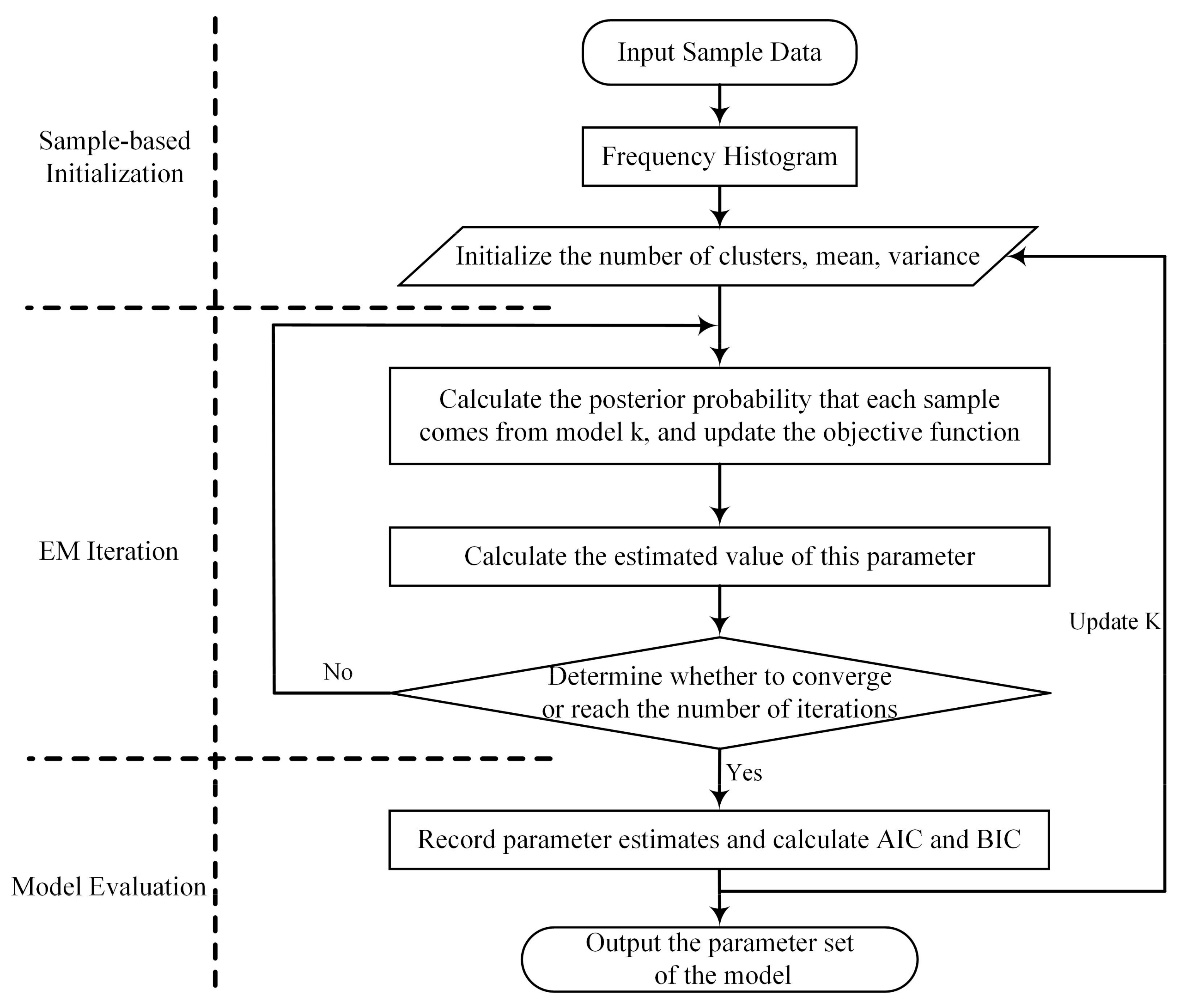
3.2.2. GMM Parameter Estimation Based on EM Algorithm

Employing the EM algorithm based on parameter estimation for the GMM, the logarithmic likelihood function [22] in Equation (4) is as follows:

$$L\left(x|\mathsf{\Theta }\right)=\sum _i\ln \sum _k{\omega }_{i,k}\frac{p\left(x_i\mid z=k,{\mu }_k,{\sigma }_k\right)p\left(z=k\right)}{{\omega }_{i,k}},$$

(6)

here, ${\omega }_{i,k}$ represents the posterior probability determined via Bayes’ Rule, and ${\alpha }_k$ denotes the prior distribution of $z$:

$${\omega }_{i,k}=p\left(z=k\mid x_i,{\mu }_k,{\sigma }_k\right).$$

(7)

The specific steps for iteratively updating $\Theta$ are as follows:

E–step: Compute the posterior probability for each sample’s affiliation with model $k$ utilizing the Gaussian mixture distributions and the prior probabilities acquired following each iteration. Subsequently, derive the most current expression for the objective function.

$$Q\left(\mathsf{\Theta },{\mathsf{\Theta }}^t\right)={\sum }_i{\sum }_k{\omega }_{i,k}^t\left(\ln {\alpha }_k-\ln {\omega }_{i,k}^t-\ln \sqrt{2\pi {\sigma }_k^2}-\frac{{\left(x_i-{\mu }_k\right)}^2}{2{\sigma }_k^2}\right),$$

(8)

${\alpha }_k$ is the prior distribution of $z$.

M–step: Determine the estimated parameters of the GMM by maximizing the objective function, resulting in updated formulations for ${\alpha }_k^{t+1}$, ${\mu }_k^{t+1}$, and ${\left({\sigma }_k^2\right)}^{t+1}$:

$$\begin{gathered} {\alpha }_k^{t+1}=\frac{\sum _i{\omega }_{i,k}^t}{N}, \\ {\mu }_k^{t+1}=\frac{\sum _i{\omega }_{i,k}^t{x}_i}{\sum _i{\omega }_{i,k}^t}, \\ {\left({\sigma }_k^2\right)}^{t+1}=\frac{\sum _i{\omega }_{i,k}{\left(x_i-{\mu }_k^{t+1}\right)}^2}{\sum _i{\omega }_{i,k}}. \end{gathered}$$

(9)

3.2.3. Model Evaluation

The Akaike Information Criterion (AIC) and Bayesian Information Criterion (BIC) [23] are utilized to ascertain the suitability of the fitted model as the optimal one [24,25]. The formal definitions for these criteria are as follows

$$\begin{gathered} \mathrm{AIC}=2k-2\ln \left(L\right), \\ \mathrm{BIC}=ln\left(n\right)k-2\mathit{ln}\left(L\right). \end{gathered}$$

(10)

Here, $k$ is the number of parameters, $L$ is the likelihood function, and $n$ is the sample size. The AIC and BIC serve as statistical criteria for model selection, with smaller values indicating superior fitting results. Both criteria incorporate penalty terms that account for the number of model parameters, but it is worth noting that the BIC employs a larger penalty term compared to the AIC. This discrepancy becomes particularly relevant in cases with an abundance of samples or when the model exhibits excessive complexity. The AIC might be prone to overfitting under these circumstances, while the BIC effectively mitigates the risk of over–complex models. To determine the optimal model, various sets of model parameters $\Theta$ are obtained through iterative processes with different K–values using $K_H$ as a reference. Subsequently, the AIC and BIC are employed to ascertain if the model under consideration best fits the data.

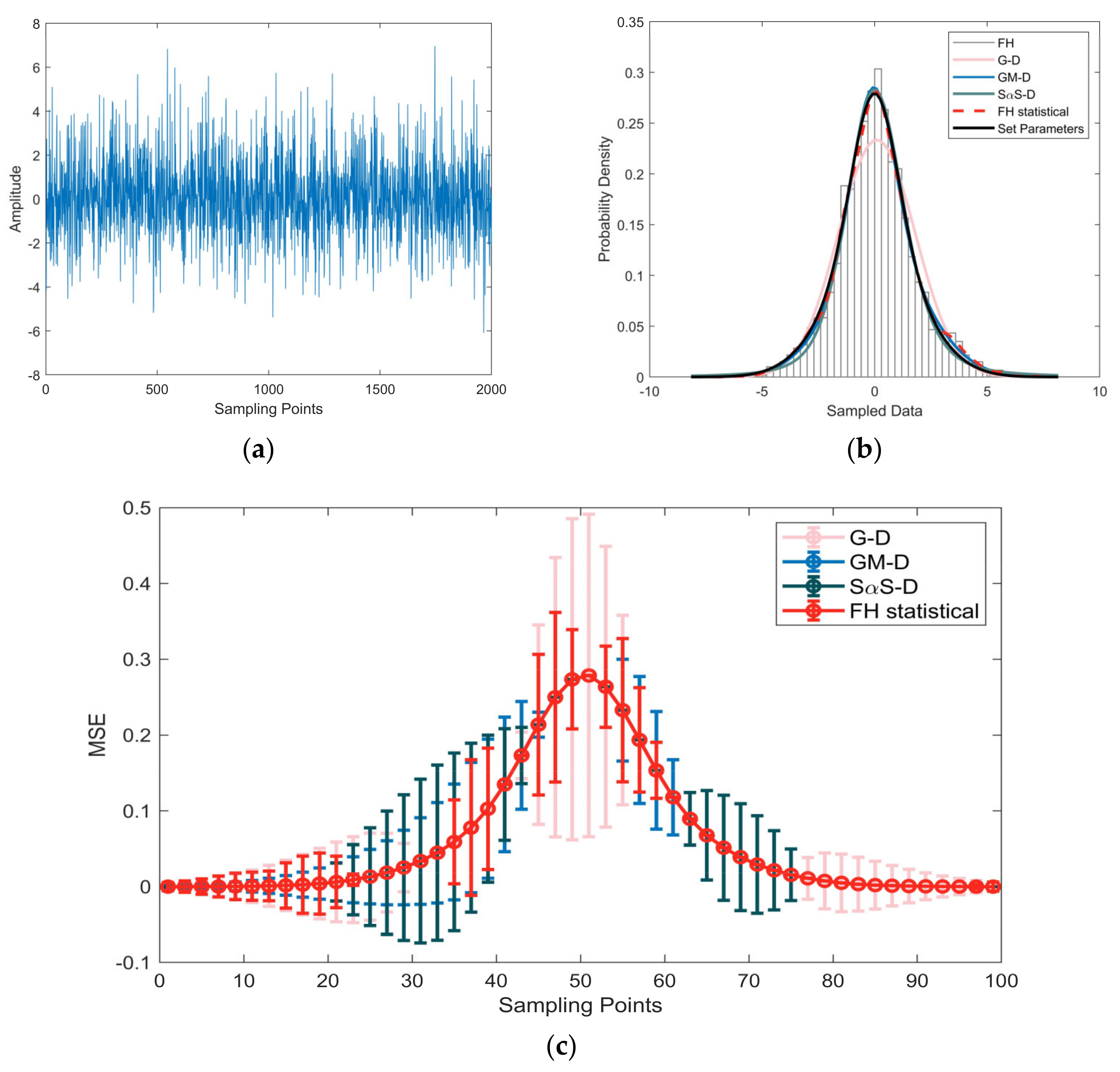
4. Simulation and Experiments Analysis

Figure 4a presents the generation of non–Gaussian random sequences using the parameter $\left[{\lambda }_i,{\mu }_i,{\mathsf{\sigma }}_i^2\right]=[0.4,0,1;0.6,0,4]$. In Figure 5a, simulated reverberation data are depicted, where the excitation signal is a Linear Frequency Modulated (LFM) signal with a pulse width of 2 milliseconds, a frequency range spanning 60–100 kHz, and a sampling frequency of 250 kHz. Figure 6a showcases a continuous wave (CW) signal with a central frequency of 4 kHz and a sampling frequency of 25 kHz. Figure 4b,c, Figure 5 and Figure 6a,b display PDF comparison plots for various models fitting the reverberation signals. Figure 4c, Figure 5 and Figure 6a–c depict comparative mean square error plots for the fitted PDF results using various models. The thick solid black line represents the true PDF curve drawn using the specified parameters. The thick red dashed line illustrates the PDF obtained through frequency histogram statistics, which can be considered an approximation of the true PDF. The pink curve denotes the PDF fitted with a Gaussian distribution and is labeled as G–D. Employing the logarithmic moment method, the PDF curve for the SαS distribution is represented in navy blue and labeled as SαS–D. The light blue curve showcases the fitting results of the GMM [26] and is denoted as GM–D. Table 1 documents the fitting results and error statistics for non–Gaussian random sequences, while Table 2 provides parameter estimation and error statistics for simulated reverberation data of the FLM signal, and Table 3 furnishes parameter estimation and error statistics for simulated reverberation data of the CW signal.

Figure 4. Waveform plot, probability density function (PDF) curve, and mean square error of non–Gaussian random sequences. (a) Waveform plot; (b) comparative PDF curves based on different models in graphical format; and (c) mean square error plots of the fitting results from different models.

Figure 5. Simulation of the reverberation data of an LFM signal, the PDF curve, and its mean square error plot. (a) Waveform plot; (b) comparative PDF curves based on different models in graphical format; and (c) mean square error plots of the fitting results from different models.

Figure 6. Simulation of the reverberation data of a CW signal, the PDF curve, and its mean square error plot. (a) Waveform plot; (b) comparative PDF curves based on different models in graphical format; and (c) mean square error plots of the fitting results from different models.

Table 1. Fitting results and statistical analysis of errors for non–Gaussian random sequences.

Distribution	G–D		SαS–D				GM–D
Parameter	$\left[\mathit{\mu },\mathit{\sigma }\right]$		$\left[\mathit{\alpha },\mathit{\beta },\mathit{\gamma },\mathit{\mu }\right]$				$\left[{\mathit{\lambda }}_{\mathit{k}},{\mathit{\mu }}_{\mathit{k}},{\mathit{\sigma }}_{\mathit{k}}\right]$
Estimation	0.096	1.710	1.579	0.149	1.011	0.141	0.648	0.185	2.015
							0.352	−0.068	0.881
MSE	2.2 × 10−4		2.4 × 10−5				1.8 × 10−5

Table 2. Parameter estimation results and error statistics of LFM signals.

Distribution	G–D		SαS–D				GM–D
Parameter	$\left[\mathit{\mu },\mathit{\sigma }\right]$		$\left[\mathit{\alpha },\mathit{\beta },\mathit{\gamma },\mathit{\mu }\right]$				$\left[{\mathit{\lambda }}_{\mathit{k}},{\mathit{\mu }}_{\mathit{k}},{\mathit{\sigma }}_{\mathit{k}}\right]$
Estimation	−0.144	0.271	1.430	0.112	−0.148	−0.123	0.385	−0.123	2.091
							0.615	−0.158	0.267
MSE	0.0420		0.0062				0.0009

Table 3. Parameter estimation results and error statistics of CW signals.

Distribution	G–D		SαS–D				GM–D
Parameter	$\left[\mathit{\mu },\mathit{\sigma }\right]$		$\left[\mathit{\alpha },\mathit{\beta },\mathit{\gamma },\mathit{\mu }\right]$				$\left[{\mathit{\lambda }}_{\mathit{k}},{\mathit{\mu }}_{\mathit{k}},{\mathit{\sigma }}_{\mathit{k}}\right]$
Estimation	−0.144	0.271	1.430	0.112	−0.148	−0.123	0.248	0.004	0.013
							0.692	0.692	0.037
							0.060	0.031	0.051
MSE	0.5546		0.0550				0.0139

Mean squared error (MSE) serves as a key metric for assessing the disparity between the actual ground truth values and the estimated values derived from the established model. MSE, as formally defined, quantifies this discrepancy as follows:

$$\mathit{MSE}=\frac{1}{N}\sum _{n=1}^N{(\theta -\widehat{\theta })}^2,$$

(11)

where $\theta$ is the ground truth PDF value, $\widehat{\theta }$ is the PDF value estimated by the model, and $N$ is the number of snapshots. Smaller MSE indicates that the predictive model is more accurate.

For the sake of model simplification, in cases where the MSE difference between two Gaussian mixture models with varying K–values is less than 5%, we consider the model with the higher K–value as exhibiting signs of overfitting.

When fitting simulated data using the GMM, preprocessing based on frequency histograms was performed with an initial cluster number of ${\mathrm{K}}_{\mathrm{H}}=1$. As shown in Figure 4b, Figure 5, Figure 6a,b, the fitting results of Gaussian distributions noticeably deviate from the true PDF, while the PDF curves of other distributions almost perfectly overlap with the curve representing the true PDF. Similarly, these results are consistently observed in Figure 7c, Figure 8, Figure 9 and Figure 10a–c. Data in Table 1, Table 2 and Table 3 suggest that the MSE for Gaussian mixture and SαS distributions is approximately one–tenth of that for Gaussian distributions. It can be inferred that for one–dimensional, zero–mean, single–peaked non–Gaussian data generated by different modulation signals (CW and FLM), SαS and Gaussian mixture distributions exhibit excellent fitting capabilities, whereas the fitting results of Gaussian distributions fall far short of expectations.

Figure 7. The reverberation data obtained in Experiment 1, along with probability density function (PDF) curves and their mean square errors. (a) Waveform plots; (b) comparative PDF curve comparisons based on different models; and (c) mean square error plots for the fitting results from different models.

Figure 8. The first section of reverberation data, PDF curves, and their mean square errors in Experiment 2. (a) Waveform plots; (b) comparative PDF curve comparisons based on different models; and (c) mean square error plots for the fitting results from different models.

Figure 9. The second section of reverberation data, PDF curves, and their mean square errors in Experiment 2. (a) Waveform plots; (b) comparative PDF curve comparisons based on different models; and (c) mean square error plots for the fitting results from different models.

Figure 10. The third section of reverberation data, PDF curves, and their mean square errors in Experiment 2. (a) Waveform plots; (b) comparative PDF curve comparisons based on different models; and (c) mean square error plots for the fitting results from different models.

5. Verification Based on the Measured Data

5.1. Method Validation

Experiment 1 was conducted at Moganshan Lake in Huzhou, China, located at latitude 30.5425° and longitude 119.9774°. This test site is specialized for conducting lake–based environmental tests, featuring a water depth of approximately 8 m and a rocky lakebed. An active sonar system was employed, equipped with independent transmitter and receiver components. The experimental setup included a Uniform Linear Array (ULA) consisting of four hydrophones, with a sampling frequency of 250 kHz and a sampling duration of 0.26 s per acquisition. The transmitted signal used a Linear Frequency Modulation (LFM) signal with a frequency range of 2 to 4 kHz. The objective of the experiment was a spherical object, with the aim of capturing its motion trajectory. Experiment 2 was carried out in the marine area near Dalian, China, situated at latitude 38.9140° and longitude 121.6146°, representing a typical marine environmental testing ground. This region is characterized by a water depth of approximately 70 m, substantial seabed sediment accumulation, and a complex environmental profile. An active sonar system with a co–located transmitter and receiver configuration was employed. In this experiment, a Uniform Linear Array (ULA) consisting of 27 hydrophones was utilized, with element spacing set at 5 mm. The ULA had a sampling frequency of 1000 kHz, and the sampling duration for each session was 0.05 s. The transmitted signal also employed a Linear Frequency Modulation (LFM) signal with a pulse width of 2 milliseconds and a frequency range of 100 to 200 kHz. The experiment targeted an unmanned underwater vehicle (UUV) model with the objective of capturing its dynamics. The typical sound velocity in water was around 1500 m per second, which is a common characteristic of complex underwater datasets. Additionally, amplitude normalization was applied to the data before modeling. It is worth noting that the Dalian region experiences complex sea conditions, abundant underwater scatterers, and strong reverberation interference, which was confirmed by subsequent waveform analysis.

Figure 7a displays the waveform of the measured reverberation data in Experiment 1, while Figure 8a, Figure 9 and Figure 10a showcase the waveforms of three distinct segments of Experiment 2’s measured reverberation data. In Figure 7b, Figure 8, Figure 9 and Figure 10a,b, PDF curves fitted by various models are presented. Figure 7c, Figure 8, Figure 9 and Figure 10a–c depict comparative mean square error plots for the fitted PDF results using various models. The gray bars within the figures represent the frequency histogram of the reverberation data, with the red dashed line depicting the PDF curve derived statistically from the frequency histogram, thus representing the true model values. The PDF curve for the Gaussian distribution is depicted by a pink curve labeled as G–D in the figures. The PDF curve fitted by the GMM is represented in sky blue and marked as GM–D in the figures, while the dark blue curve corresponds to the PDF of the SαS distribution and is denoted as SαS–D in the figures.

5.2. Analysis of Results

Table 4 provides an overview of the values for ${\mathrm{K}}_{\mathrm{H}}$, ${\mathrm{K}}_{\mathrm{AIC}}$, ${\mathrm{K}}_{\mathrm{BIC}}$, and ${\mathrm{K}}_{\mathrm{B}}$, and MSE corresponding to the four distinct sets of reverberation data. In Table 5, the parameter estimation results for modeling the reverberation data using various models are detailed. Table 6 focuses on the mean squared error (MSE) associated with each model. Analysis of Table 4 reveals that the optimal order for the GMM obtained through both the AIC and BIC is consistent. Specifically, concerning the reverberation data presented in Figure 6a, the AIC algorithm determines the optimal GMM order to be 6, with a marginal 1.6‰ difference in MSE when compared to the GMM model with a cluster number of 3. For the reverberation data in Figure 7a, the MSE of fitting results with the GMM orders 5 and 3 varies by a slight 1.2‰. In the dataset featured in Figure 9a, the GMM fitting results indicate a minuscule 0.7‰ difference in MSE between clusters 6 and 5. In all these instances, the MSE remains below 5‰, and for the sake of model simplification, the smaller K–value is favored as the optimal model order.

Table 4. GMM fitting results with different K–values and their MSE.

Data	Figure 6a	Figure 7a	Figure 8a	Figure 9a
$K_H$	1	1	3	3
$K_H-MSE$	0.0107	0.0170	0.0189	0.0230
$K_{AIC}$	6	5	4	6
$K_{AIC}-MSE$	0.0015	0.0015	0.0013	0.0006
$K_{BIC}$	6	5	4	6
$K_{BIC}-MSE$	0.0031	0.0015	0.0013	0.0006
$K_B$	3	3	4	5
$K_H-MSE$	0.0031	0.0027	0.0013	0.0013

Table 5. Fitting results of different distributions to reverberation data.

Parameter	SαS–D [$\mathsf{\alpha },\mathsf{\beta },\mathsf{\gamma },\mathsf{\mu }$]				GM–D [${\mathsf{\lambda }}_{\mathit{k}}{,\mathsf{\mu }}_{\mathit{k}},{\mathsf{\sigma }}_{\mathit{k}}$]
Data
Figure 6a	1.627	0.151	0.133	0.024	0.767	0	0.023
					0.206	0.0138	0.015
					0.027	−0.037	0.100
Figure 7b	1.077	0.030	0.112	0.093	0.741	−0.087	0.149
					0.254	−0.096	0.057
					0.005	−0.656	0.253
Figure 8b	1.606	−0.028	0.09	−0.09	0.514	0.062	0.098
					0.061	−0.062	0.281
					0.354	0.077	0.253
					0.061	0.782	0.096
Figure 9b	1.537	0.010	0.220	0.053	0.255	0.420	0.196
					0.036	0.847	0.068
					0.032	−0.752	0.059
					0.372	0.060	0.115
					0.305	−0.272	0.221

Table 6. Error statistics for various estimated distribution parameters.

Data	Figure 6b	Figure 7b	Figure 8b	Figure 9b
MSE
G–D	0.0107	0.0170	0.1525	0.0245
SαS–D	0.0037	0.0057	0.0088	0.0159
GM–D	0.0031	0.0027	0.0013	0.0013

Observing the PDF curve comparison charts in Figure 6b, Figure 7, Figure 8 and Figure 9a,b, it becomes evident that the reverberation data acquired in a complex measured environment exhibit substantial deviations in the fitting results when employing a Gaussian distribution. For the reverberation data conforming to a zero mean and a single bell–shaped distribution, as depicted in Figure 6b and Figure 7b, both the Gaussian Mixture Model (GMM) and SαS distributions exhibit excellent fitting capabilities for the data’s PDF curve, with MSE values of less than 3‰. However, when dealing with reverberation data characterized by multiple peaks and non–zero mean, as demonstrated in Figure 8b and Figure 9b, the SαS distribution can only adequately fit the data associated with the primary peak, resulting in an error exceeding 5‰. Conversely, the PDF curve fitted by the GMM aligns closely with the true value. Table 6 data further emphasize the suitability of the GMM for reverberation fitting, as they demonstrate a maximum error of 3.1‰. In contrast, the SαS distribution exhibits a maximum error of 15.9‰, while the Gaussian distribution’s error exceeds 10‰, with a maximum reaching 152‰. Similarly, these results are consistently observed in Figure 7c, Figure 8, Figure 9 and Figure 10a–c, highlighting the minimal error associated with the GMM and the maximum error exhibited by the Gaussian model. These findings underscore the superiority of the GMM in accurately modeling reverberation data in diverse scenarios.

6. Conclusions

In this study, the GMM was employed to statistically characterize the distribution characteristics of reverberation data. Prior to applying the expectation–maximization (EM) algorithm for parameter estimation, data preprocessing was utilized to mitigate the limitations associated with random parameter initialization, which can lead to convergence towards suboptimal solutions and require extensive computational resources. Through a systematic comparison of different cluster numbers, we effectively addressed the issue of overfitting in the Akaike Information Criterion (AIC) algorithm within an acceptable error margin, consequently reducing the model’s complexity. The validation, using both simulated and real measured reverberation data, demonstrated that both the SαS distribution and GMM models offer robust modeling capabilities for single–peaked, zero–mean reverberation data. In this context, the mean squared error (MSE) of the GMM was less than 4‰, representing less than a tenth of the MSE achieved by a Gaussian distribution. However, when dealing with reverberation data exhibiting multi–peaked distributions and non–zero means, the GMM outperformed other distributions in terms of probability density fitting. Specifically, the MSE of the GMM was less than 2‰, whereas the SαS distribution exceeded 8‰, and the Gaussian distribution exceeded 24‰. The experimental results clearly demonstrate that the GMM offers superior probability density fitting for measured reverberation data in complex environments, showcasing its broader applicability.

References

1. Wang, L.; Wang, Q. The influence of marine biological noise on sonar detection. In Proceedings of the 2016 IEEE/OES China Ocean Acoustics (COA), Harbin, China, 9–11 January 2016. [Google Scholar]
2. Tian, T. Shengna Jishu, 2nd ed.; Harbin Engineering University Press: Harbin, China, 2009. [Google Scholar]
3. Faure, P. Theoretical Model of Reverberation Noise. J. Acoust. Soc. Am. 1964, 36, 259–266. [Google Scholar] [CrossRef]
4. Olishevski, B. Statistical Characteristics of Sea Reverberation, 2nd ed.; Science Press: Beijing, China, 1977. [Google Scholar]
5. Middleton, D. New physical–statistical methods and models for clutter and reverberation: The ka–distribution and related probability structures. IEEE J. Ocean. Eng. 1999, 24, 261–284. [Google Scholar] [CrossRef]
6. Pernkopf, F.; Bouchaffra, D. Genetic–based EM algorithm for learning gaussian mixture models. IEEE Trans. Pattern Anal. Mach. Intell. 2005, 27, 1344–1348. [Google Scholar] [CrossRef] [PubMed]
7. Wei, H.; Wang, P. Gaussian mixture model for reverberation. Tech. Acoust. 2007, 26, 514–518. [Google Scholar]
8. Wang, P.; Wei, H.; Lou, L. Oceanic reverberation probability density modeling based on symmetric alpha–stable distribution. J. Harbin Eng. Univ. 2021, 42, 55–60. [Google Scholar]
9. Liu, W.; Wang, P.; Gu, X. Comparison of two EM algorithms for gaussian mixture parameter estimation. Tech. Acoust. 2014, 33, 539–543. [Google Scholar]
10. Liu, M.; Yu, Z. An improved expectation–maximum algorithm. J. Jilin Univ. (Sci. Ed.) 2022, 60, 1176–1182. [Google Scholar]
11. Najar, F.; Bourouis, S.; Bouguila, N. A comparison between different gaussian–based mixture models. In Proceedings of the 2017 IEEE/ACS 14th International Conference on Computer Systems and Applications (AICCSA), Hammamet, Tunisia, 30 October–3 November 2017. [Google Scholar]
12. He, W.; Yu, R.; Zheng, Y.; Jiang, T. Image denoising using asymmetric gaussian mixture models. In Proceedings of the 2018 International Symposium in Sensing and Instrumentation in IoT Era (ISSI), Shanghai, China, 6–7 September 2018. [Google Scholar]
13. Przyborowski, M.; Ślęzak, D. Approximation of the expectation–maximization algorithm for gaussian mixture models on big data. In Proceedings of the 2022 IEEE International Conference on Big Data (Big Data), Kyoto, Japan, 13–16 December 2022. [Google Scholar]
14. Ma, B.; Gong, L.; Chen, X.; Liu, G. Study of characteristics of acoustic intensity in acoustic vector ocean reverberation based on CW pulse. J. Nav. Univ. Eng. 2022, 34, 102–106. [Google Scholar]
15. Ivakin, A.N.; Williams, K.L. Midfrequency acoustic propagation and reverberation in a deep ice–covered arctic ocean. J. Acoust. Soc. Am. 2022, 152, 1035–1044. [Google Scholar] [CrossRef] [PubMed]
16. Cao, F.; Zhang, X.; Han, J. Experimental analysis of statistical property of low frequency reverberation envelope in shallow water. In Proceedings of the 2021 OES China Ocean Acoustics, Heilongjiang, China, 14–17 July 2021. [Google Scholar]
17. Wang, J.; Wang, C.; Cheng, T. Active sonar reverberation suppression based on beam space data normalization. In Proceedings of the 2017 IEEE International Conference on Signal Processing, Communications and Computing, Xiamen, China, 22–25 October 2017. [Google Scholar]
18. Li, Q. Introduction to Sonar Signal Processing, 2nd ed.; Chinese Academy of Sciences: Beijing, China, 2000. [Google Scholar]
19. Glodek, M.; Schels, M.; Schwenker, F. Ensemble gaussian mixture models for probability density estimation. Comput. Stat. 2013, 28, 127–138. [Google Scholar] [CrossRef]
20. Guo, H.; Chu, F.; Zhu, D. Research on gaussian mixture auto–regressive reverberation modeling and whitening algorithm. In Proceedings of the 2021 IEEE International Conference on Signal Processing, Communications and Computing, Xi’an, China, 17–20 August 2021. [Google Scholar]
21. Jovanović, A.; Perić, Z.; Nikolić, J. The effect of uniform data quantization on GMM–based clustering by means of EM algorithm. In Proceedings of the 2021 20th International Symposium INFOTEH–JAHORINA, Sarajevo, Bosnia and Herzegovina, 17–19 March 2021. [Google Scholar]
22. Kasim, F.A.B.; Pheng, H.S.; Nordin, S.Z.B. Gaussian mixture modelexpectation maximization algorithm for brain images. In Proceedings of the 2021 2nd International Conference on Artificial Intelligence and Data Sciences (AiDAS), Kuala Lumpur, Malaysia, 8–9 September 2021. [Google Scholar]
23. Stepashko, V. Asymptotic properties of a class of criteria for best model selection. In Proceedings of the 2020 IEEE 15th International Conference on Computer Sciences and Information Technologies, Zbarazh, Ukraine, 23–26 September 2020. [Google Scholar]
24. Wei, J.; Zhou, L. Model selection using modified AIC and BIC in joint modeling of paired functional data. Stat. Probab. Lett. 2010, 80, 1918–1924. [Google Scholar] [CrossRef]
25. Ding, J.; Tarokh, V.; Yang, Y. Bridging AIC and BIC: A new criterion for autoregression. IEEE Trans. Inf. Theory 2017, 64, 4024–4043. [Google Scholar] [CrossRef]
26. Mo, X.; Wen, H.; Yang, Y. A parameter estimation method of α stable distribution and its application in the statistical modeling of ice–generated noise. Acta Acust. 2023, 48, 319–326. [Google Scholar]