Article

Utilizing Multivariate Adaptive Regression Splines (MARS) for Precise Estimation of Soil Compaction Parameters

by
Musaab Sabah Abed
1,
Firas Jawad Kadhim
1,
Jwad K. Almusawi
1,
Hamza Imran
2,
Luís Filipe Almeida Bernardo
3,* and
Sadiq N. Henedy
4
1
Department of Civil Engineering, Faculty of Engineering, University of Misan, Amarah 62001, Iraq
2
Department of Environmental Science, College of Energy and Environmental Science, Alkarkh University of Science, Baghdad 10081, Iraq
3
Department of Civil Engineering and Architecture, GeoBioTec-UBI, University of Beira Interior, 6201-001 Covilhã, Portugal
4
Department of Civil Engineering, Mazaya University College, Nasiriyah City 64001, Iraq
*
Author to whom correspondence should be addressed.
Appl. Sci. 2023, 13(21), 11634; https://doi.org/10.3390/app132111634
Submission received: 8 October 2023 / Revised: 21 October 2023 / Accepted: 23 October 2023 / Published: 24 October 2023
(This article belongs to the Special Issue The Application of Machine Learning in Geotechnical Engineering)

Abstract

:
Traditional laboratory methods for estimating soil compaction parameters, such as the Proctor test, have been recognized as time-consuming and labor-intensive. Given the increasing need for the rapid and accurate estimation of soil compaction parameters for a range of geotechnical applications, the application of machine learning models offers a promising alternative. This study focuses on employing the multivariate adaptive regression splines (MARS) model algorithm, a machine learning method that presents a significant advantage over other models through generating human-understandable piecewise linear equations. The MARS model was trained and tested on a comprehensive dataset to predict essential soil compaction parameters, including optimum water content (wopt) and maximum dry density (ρdmax). The performance of the model was evaluated using coefficient of determination (R2) and root mean square error (RMSE) values. Remarkably, the MARS models showed excellent predictive ability with high R2 and low RMSE, MAE, and relative error values, indicating its robustness and reliability in predicting soil compaction parameters. Through rigorous five-fold cross-validation, the model’s predictions for wopt returned an RMSE of 1.948%, an R2 of 0.893, and an MAE of 1.498%. For ρdmax, the results showcased an RMSE of 0.064 Mg/m3, an R2 of 0.899, and an MAE of 0.050 Mg/m3. When evaluated on unseen data, the model’s performance for wopt prediction was marked with an MAE of 1.276%, RMSE of 1.577%, and R2 of 0.948. Similarly, for ρdmax, the predictions were characterized by an MAE of 0.047 Mg/m3, RMSE of 0.062 Mg/m3, and R2 of 0.919. The results also indicated that the MARS model outperformed previously developed machine learning models, suggesting its potential to replace conventional testing methods. The successful application of the MARS model could revolutionize the geotechnical field through providing quick and reliable predictions of soil compaction parameters, improving efficiency for construction projects. Lastly, a variable importance analysis was performed on the model to assess how input variables affect its outcomes. It was found that fine content (Cf) and plastic limit (PL) have the greatest impact on compaction parameters.

1. Introduction

Soil compaction, a foundational process in geotechnical engineering, refers to the method of tightening soil particles and reducing air voids, thereby increasing density while maintaining the existing water content [1]. This technique not only enhances soil’s mechanical behavior but also provides a stable base for various infrastructures, solidifying its significance in the field of civil engineering. Initially suggested by Proctor in 1933 [2], soil compaction involves applying specified compactive effort in a controlled laboratory setting, allowing for various water contents. This process enables engineers to pinpoint the optimal moisture content and maximum dry density—two essential parameters obtained from the compaction curve [3,4,5]. In field compaction, the key parameters are the optimum water content (wopt) and maximum dry density (ρdmax). These are crucial in determining the maximum dry density of soil, which indicates an enhanced soil bearing capacity. The optimum water content is the specific moisture level at which soil can attain its highest dry density following a certain compaction effort. It is the minimum water necessary to form a thin film on soil particles, aiding their sliding movement for compaction. Compressing soil to its greatest theoretical density involves eliminating gases within the soil via expelling them through voids in the soil matrix. This process of gas expulsion is fundamental to soil densification, allowing soil to reach its maximum potential density. Hence, wopt and ρdmax are vital in achieving the desired soil densification and stability [6]. These parameters form the backbone of long-term performance for a myriad of geotechnical structures, such as landfill liners, highway embankments, railway track-beds, earth dams, nuclear waste disposal facilities, and airfield pavements [7,8,9,10,11,12,13,14,15,16,17]. For example, study [7] found that wopt and ρdmax are crucial factors affecting the compression of compacted Oklahoma soils, influencing collapse potential in embankments. Another study [8] used wopt and ρdmax as critical parameters to understand the behavior and performance of MX80, which is a versatile clay for nuclear waste barriers. Furthermore, study [14] investigated the microstructure and hydraulic properties of high-speed railway subgrade soil using different values of wopt and ρdmax to understand its behavior. Thus, accurately predicting and understanding the compaction parameters of diverse soil types is paramount for the successful construction and maintenance of these geotechnical structures.
To find compaction parameters, two main compaction approaches emerged: the standard Proctor compaction and the modified Proctor compaction [1]. The standard method is typically adopted for regular traffic loading situations, while the modified approach is used when dealing with heavy unit weights like those considered for airfield pavements. Outcomes derived from laboratory tests conducted using either the standard Proctor compaction method (ASTM D698) [18] or the modified Proctor compaction method (ASTM D1557) [19] are visually represented via an inverted ‘V’ curve. This graphical representation illustrates the peak, known as ρdmax, and the corresponding moisture content, termed as the wopt of the soil. Reaching the optimum moisture content and maximum dry density in a laboratory setting, using both standard and modified compaction tests, demands significant resources. It involves a considerable amount of time (typically 2–3 days), substantial effort, and a large volume of soil (around 20 kg per individual test) [1]. Efforts have been made to overcome this challenge through proposing several prediction models for determining the soil compaction parameters more efficiently. Empirical equations, created via multiple linear regression, can predict wopt and ρdmax of soil [20,21,22,23,24,25]. These models offer the benefits of quick calculations and easy application, which speed up decision-making in geotechnical projects. They are user-friendly, making them accessible to a variety of users, not just experts. However, these models come with several limitations. One issue is the existence of numerous equations for the same factors, leading to potential confusion and inconsistency in results. This vast array of options makes the selection of the appropriate model challenging, possibly affecting the reliability of predictions. Another significant limitation is the assumption of linear behavior, which often does not reflect the complex, often non-linear nature of soil behavior. These models, while providing an estimation, might not fully encapsulate the range of outcomes in different conditions due to their simplified assumptions.
The complex nature of soil compaction parameters, influenced by numerous interrelated parameters, necessitates the use of robust, data-driven methodologies such as artificial intelligence. Traditional models struggle to capture these intricate relationships, but artificial intelligence and other data-driven methods have shown proficiency in navigating the inherent non-linearity and successfully estimating soil compaction parameters. Continued research should focus on employing precise and reliable techniques, like artificial intelligence, that can effectively handle these complexities. In the area of predicting soil compaction parameters, several studies have demonstrated noteworthy advancements. The use of artificial neural networks (ANNs) has been successfully employed in various models. For instance, one investigation applied an ANN to model wopt and ρdmax in soil stabilized with nanomaterials. The model exhibited impressive prediction accuracy of over 97%, surpassing conventional statistical models [26]. Extending this approach to different soil types, another study harnessed the potential of deep neural networks to predict soil compaction parameters specific to Egyptian soil. The study achieved remarkable accuracy, with R2 values of 0.864 for ρdmax and 0.924 for wopt, thereby surpassing the performance of a simple artificial neural network with just one hidden layer [27]. In the context of highway projects, a multi-layer perceptron neural network model was developed to predict modified compaction parameters for both coarse and fine-grained soil samples. This model, similar to its predecessors, delivered highly accurate results [28]. Stepping beyond traditional ANNs, a novel hybrid intelligence paradigm known as the ANFIS-IGWO model was proposed in a different study. This model demonstrated superior precision in predicting soil compaction parameters, boasting correlation values of 0.9203 and 0.9050 for wopt and ρdmax, respectively [29]. This accuracy was found to surpass other hybrid ANFIS models. In yet another study, an ANN was utilized to develop predictive equations for the Proctor compaction parameters of fine-grained soil [30]. The resulting ANN model demonstrated high efficiency and accuracy, particularly in predicting unseen datasets, thus setting a new standard compared to existing models in the literature. Moving towards the integration of empirical correlations with machine learning algorithms, one paper investigated the use of the support vector machine algorithm to predict soil compaction properties [31]. This approach aimed at significantly reducing the time and effort required in the laboratory, achieving R2 values of 0.86 and 0.91 for wopt and ρdmax, respectively. Lastly, in a significant stride towards machine learning models, a novel model called “ComPara2021” was proposed [17]. This model, based on machine learning, demonstrated superior performance in predicting soil compaction parameters compared to its contemporaries, proving the value of such models in saving both time and cost.
Another form of artificial intelligence is genetic programming approaches such as gene expression programming (GEP) and multigene expression programming (MEP). GEP and MEP are advantageous frameworks that integrate the benefits of both genetic programming and genetic algorithms, enabling them to evaluate more complex functions that express the relationship between input and output data [32,33]. The GEP and MEP models have notably demonstrated their effectiveness in predicting a variety of parameters related to compacted soil [15,34,35].
The multivariate adaptive regression splines (MARS) technique, a form of artificial intelligence, offers potential benefits to geotechnical engineers. Besides being adept at tackling prediction problems, MARS can identify key input parameters that significantly influence output parameters. It also allows for the exploration of intricate nonlinear relationships between a response variable and various predictive variables—a crucial aspect in analyzing and designing soil compaction parameters. This technique has seen successful implementations in diverse fields of geotechnical engineering, including ultimate pile bearing capacity [36], the elastic modulus of rocks [37], Slope reliability analysis [38], the compressive strength of soil [39], liquefaction [40], settlement prediction [41], and penetration resistance in clay [42]. Yet, despite its proven effectiveness in these areas, its application in compaction-related studies remains surprisingly limited.
In this research, MARS is utilized to estimate the optimal moisture content (wopt) and maximum dry density (ρdmax) of compacted soil. MARS addresses the limitations of the multiple linear regression (MLR) method, as it does not necessitate an a priori form of equation between dependent and independent variables and can precisely capture complex and nonlinear relationships between inputs and outputs [43]. Unlike techniques like the ANN, which often operate as a “black box,” MARS can provide an explicit equation linking inputs and outputs [44,45,46]. This transparency has led to its frequent application in modeling intricate engineering issues. Finally, MARS successfully mitigates one of the key drawbacks of GEP and MEP, which tend to produce highly nonlinear mathematical relations between input and output data [46].

2. Research Significance

This research carries significant implications in the field of soil engineering and artificial intelligence applications. It provides a robust foundation for understanding and predicting soil compaction parameters across a variety of soil classifications. Firstly, this study is rooted in comprehensive literature-based data collection, which has amassed an extensive database of different soil types, including gravel, sand, silt, and clay. This broad spectrum of data offers a detailed and diverse basis for analysis and prediction. Secondly, we employed the MARS model to predict soil compaction parameters. To enhance the accuracy and reliability of predictions, we further fine-tuned the MARS model’s performance via hyperparameter tuning. Thirdly, we conducted a comparative study to evaluate the performance of the MARS model against other existing empirical and artificial intelligence models. This comparison seeks to identify the most effective and accurate model for predicting soil compaction parameters, contributing to the optimization of methodologies in this area of research. Lastly, we carried out a sensitivity analysis to determine the relative influence of each input variable on the scour depth. Through identifying the most impactful variables, this study aids in refining the prediction model and enhances the overall understanding of the relationships between different factors.

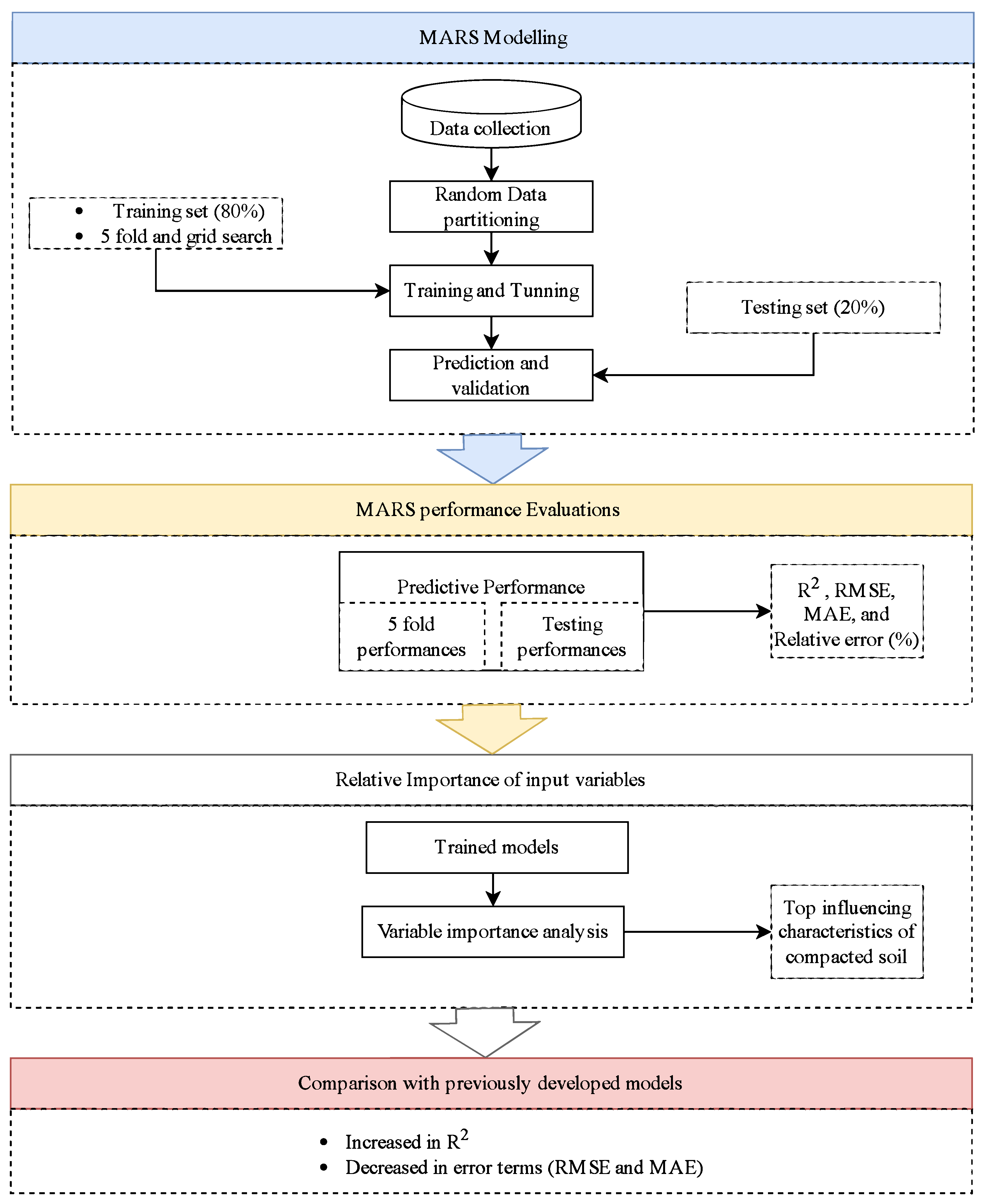
3. Materials and Methods

3.1. Research Methodology

The comprehensive research approach employed in this study is depicted in Figure 1, encompassing five fundamental phases: gathering and assimilating data, visualizing and statistically assessing the data, carrying out data modeling and analysis, evaluating the performance of machine learning (ML) models, and comparing the findings with earlier research. The data modeling and analysis are conducted using R-project, a programming framework extensively used for data mining and ML applications [47].

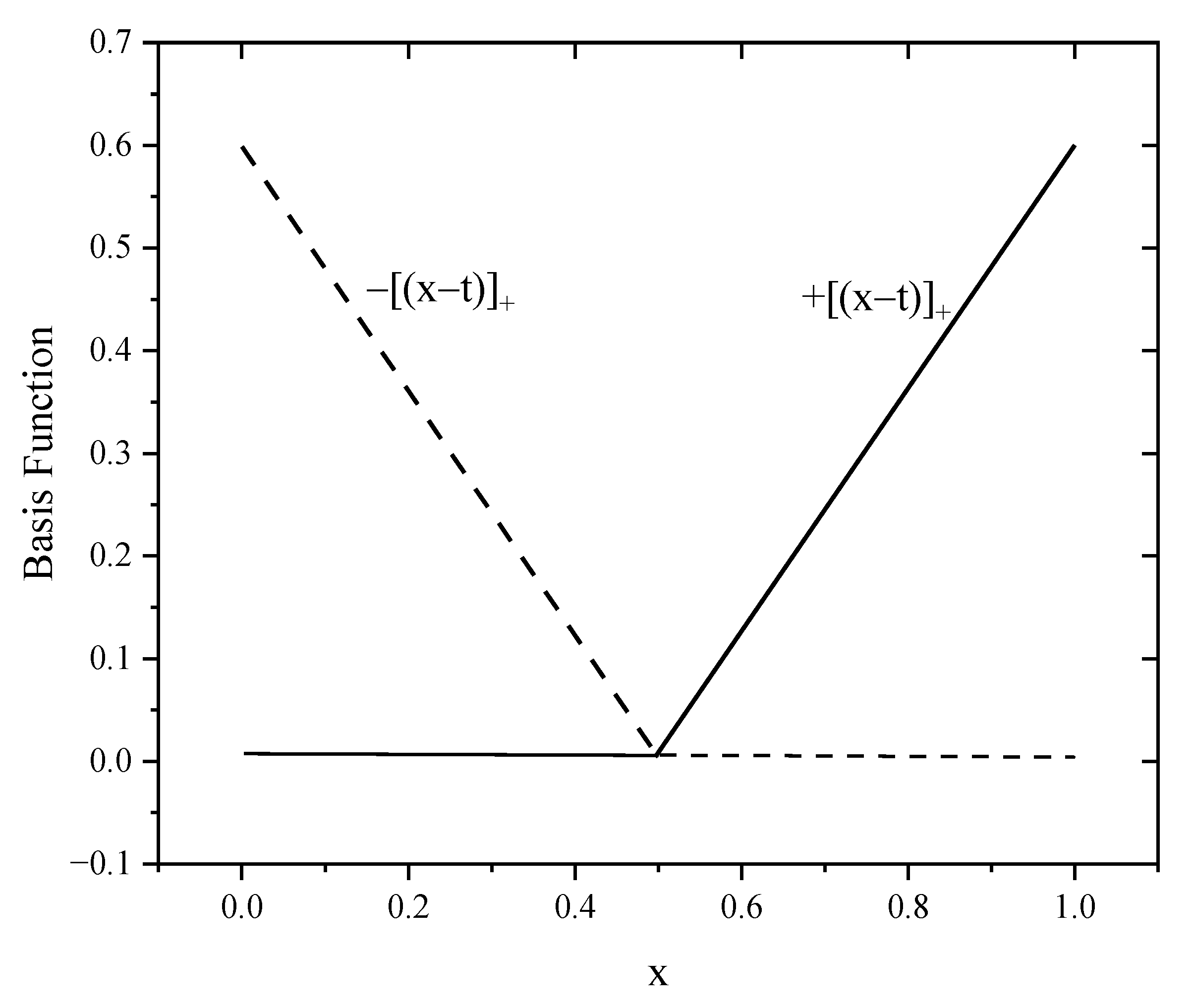
3.2. Multivariate Adaptive Regression Splines (MARS)

In the year 1991, the concept of multivariate adaptive regression splines (MARS), a method for non-parametric regression, was proposed by Friedman [48]. This approach aims to model a relationship between a set of predictor variables, represented as X (n × p), and a target variable, denoted as y (n × 1). Where n is the number of observations or samples, p is the number of predictor variables or features, X is the matrix of predictor variables with size n × p, and y is the column vector of the target variable with size n × 1. The MARS model’s mathematical representation can be expressed through the equation below:
y = f ( X ) + e
The term f(X) represents the prediction or approximation of the target variable y given the predictor variables X by the MARS model. The equation also gives us a residual vector, e (n × 1), which forms an integral part of this model. MARS can be considered as a sophisticated extension of the Classification and Regression Trees (CART) [49] technique, but it stands apart from conventional parametric methods. While parametric methods necessitate a predefined functional correlation between predictor and target variables, MARS refrains from such presumptions. Instead, MARS utilizes the predictor variables present in the specified dataset to produce a set of coefficients and piece-wise polynomials that carry the power q . These polynomials are specifically generated to encapsulate the relationship among variables, which may exhibit either a linear or a non-linear nature. These polynomials, referred to as ‘splines’, are seamlessly connected to assemble the complete MARS model. Moreover, the process of fitting these splines involves segmenting the data points of the independent variables into discrete regions, with the knot locations symbolized by ‘ t ’. The power ‘ q ’ of these splines essentially determines their linearity or non-linearity. For any variable ‘ x ’, the MARS model calculates these splines through applying the particular equations below:
[ ( x t ) ] + q = ( t x ) q , if x < t 0 , otherwise
[ + ( x t ) ] + q = ( t x ) q , if x t 0 , otherwise
In the given equations, ‘ q ’ is not less than zero, and it is a key factor in shaping the smoothness of the ultimate MARS model. In this particular investigation, ‘ q ’ is set to 1, signifying the analysis of linear splines. Figure 2 illustrates two splines related to an individual variable ‘ x ’, having ‘ q ’ set to 1 and a defined knot ‘ t ’. The left spline provides positive outcomes, while the right spline produces zero for ‘ x ’ values on the left side of the knot. On the flip side, when ‘ x ’ values lie on the right side of the knot, the right spline gives positive results, and the left spline is zero. These splines, also called as the foundation functions for ‘ x ’, play a significant role in the MARS technique. The MARS model related to the aim variable ‘y’ is formed via including a series of ‘M’ basis functions, as demonstrated in the following equation:
y ^ = f ^ M ( x ) = a o + m = 1 M a m B m ( x )
Equation (4) depicts y ^ as the target variable, which the MARS model predicts. The term ‘ a o ’ signifies the intercept term, which is a fixed constant. ‘ B m ( x ) ’ denotes the mth basis function, which could be an individual basis function or a combination of multiple basis functions, while ‘ a m ’ symbolizes the coefficient that corresponds to the mth basis function. The estimation of these coefficients is achieved via the least squares method.
The MARS model, as represented by Equation (4), is formulated using a biphasic methodology that encompasses a forward pass and a backward pass. The initial phase, known as the forward pass, involves integrating the predictor variables into the model and fine-tuning the positions of their corresponding knots. This process gives rise to the creation of double-sided basis functions, one for each predictor. In the context of an X matrix, composed of ‘n’ samples and ‘p’ predictors, ‘ n × p ’ pairs of basis functions emerge, as exhibited in Equations (2) and (3). These functions are associated with knots, denoted by x i j , where ‘ i ’ ranges from 1 to ‘n’ and ‘ j ’ spans from 1 to ‘ p ’. Every single data point affiliated with a predictor variable is taken into account as a possible knot for that variable’s pair of basis functions. However, the forward pass process often results in the formulation of a convoluted model that tends to overfit, hence reducing its predictive capability. To address this issue, the second phase, or the backward pass, is implemented. During this phase, the model is systematically simplified through sequentially eliminating the least contributing, and therefore redundant, basis functions. The backward pass continues until an optimized sub-model is achieved, characterized by its lowest Generalized Cross Validation (GCV). This enhancement substantially boosts the predictive prowess of the MARS model. The computation for determining the GCV follows the formula provided below:
G C V M = 1 n i = 1 n y i f M ( x ^ i ) 2 1 M + d × M 1 / 2 n 2

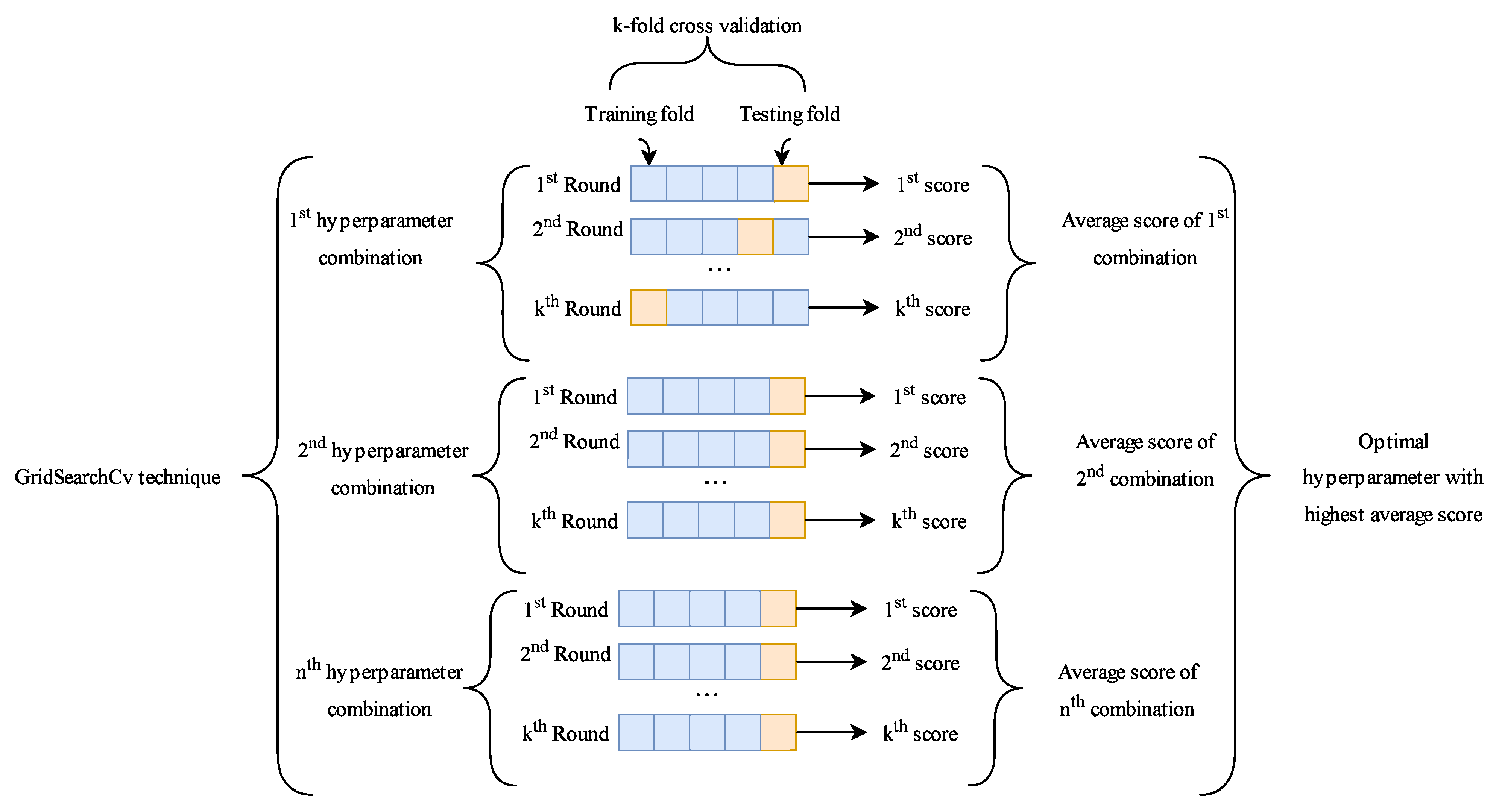
3.3. Hyperparameter Tuning Procedure

In this research, we utilized a combination of hyperparameter tuning, taking advantage of the grid search approach [50], along with cross-validation (CV) strategies. The grid search methodology essentially provides an ideal setting for parameters through arranging all variable grids within the space of the parameters. Each grid’s axis corresponds to a parameter of the algorithm, with a unique set of parameters at each grid point that requires optimization. The primary benefit of combining grid search with CV is to pinpoint the most suitable hyperparameters for the model based on the selected evaluation metric. Furthermore, this integration guarantees that the model’s performance is evaluated across various data subsets, resulting in a more robust and dependable assessment of its efficacy. A potential drawback of this methodology is that it is computationally intensive. The model needs to be trained ‘k’ times, which can be time-consuming for large datasets or complex models. However, since our data only has 226 points, the computational demand in our specific case is considerably reduced, making the method more manageable and feasible for our dataset size. To ensure the unbiased selection of data, we employed a prevalent validation method known as k-fold CV [51,52,53,54,55] during the tuning process of hyperparameters for MARS models. K-fold CV, a standard type of CV, is extensively used in machine learning. Although there is no definitive rule for choosing the value of K, in practical machine learning scenarios, K is commonly set at 5 or 10. According to Rodriguez [56], the bias in an accurate estimation is likely to be reduced when the fold count is either 5 or 10. Based on this and the suggestions of Kohavi [57] and Wong [58], we chose 5 for K. This decision also took into consideration the trade-off between computational efficiency and bias. As a result, five different sets of training and validation runs were performed, with the outcomes being averaged to depict the overall performance of the MARS models on the training dataset. All the data-related operations in this study were handled using R software 4.1.3 (R Core Team, Vienna, Austria) [47]. The approach for hyperparameter tuning used in this research for training the model and selecting hyperparameters is depicted in Figure 3, as illustrated in reference [59].
Our research made use of the R package “earth” to perform MARS modeling. This implementation called for the user’s careful consideration of two particular tuning parameters: “degree” and “nprune”. The “degree” parameter indicates the highest degree of interaction allowed in the model. By default, this value is set to 1, leading to the creation of a MARS model that is additive and lacks interaction terms. However, it is noteworthy that MARS is capable of building models that encompass interactions of a degree of two or even higher. Despite this capability, a guideline suggested by Hastie et al. [60] recommends maintaining an upper limit on the degree of interaction. The benefit of keeping a lower degree of interaction lies in its ability to assist in interpreting the final model in a more straightforward manner. On the other hand, a higher degree of interaction could potentially cause occasional volatility in the model’s predictive capabilities, possibly causing predictions to deviate significantly from actual values. Hence, to evaluate the impact of varying degrees of interaction, we experimented with three different values: 1, 2, and 3. The second parameter, “nprune”, signifies the maximum number of terms (inclusive of the intercept) that can be present in the model. The “nprune” value should be equal to or greater than 2 and less than “nk”. Here, “nk” stands for the maximum number of terms in the model before any pruning activity is initiated. This value of “nk” is determined by the formula nk = min (200, max (20, 2 × ncol(x))) + 1, where ncol(x) is the total number of predictive variables. For our specific study, which involved a total of 6 predictive variables, we looked into 20 potential values for nprune, ranging from 2 to 20. The process of constructing and evaluating these 57 MARS models, featuring degrees of 1, 2, 3 and nprune values ranging from 2 to 20, was accomplished through the implementation of a five-fold cross-validation procedure.

3.4. Performance Metrics
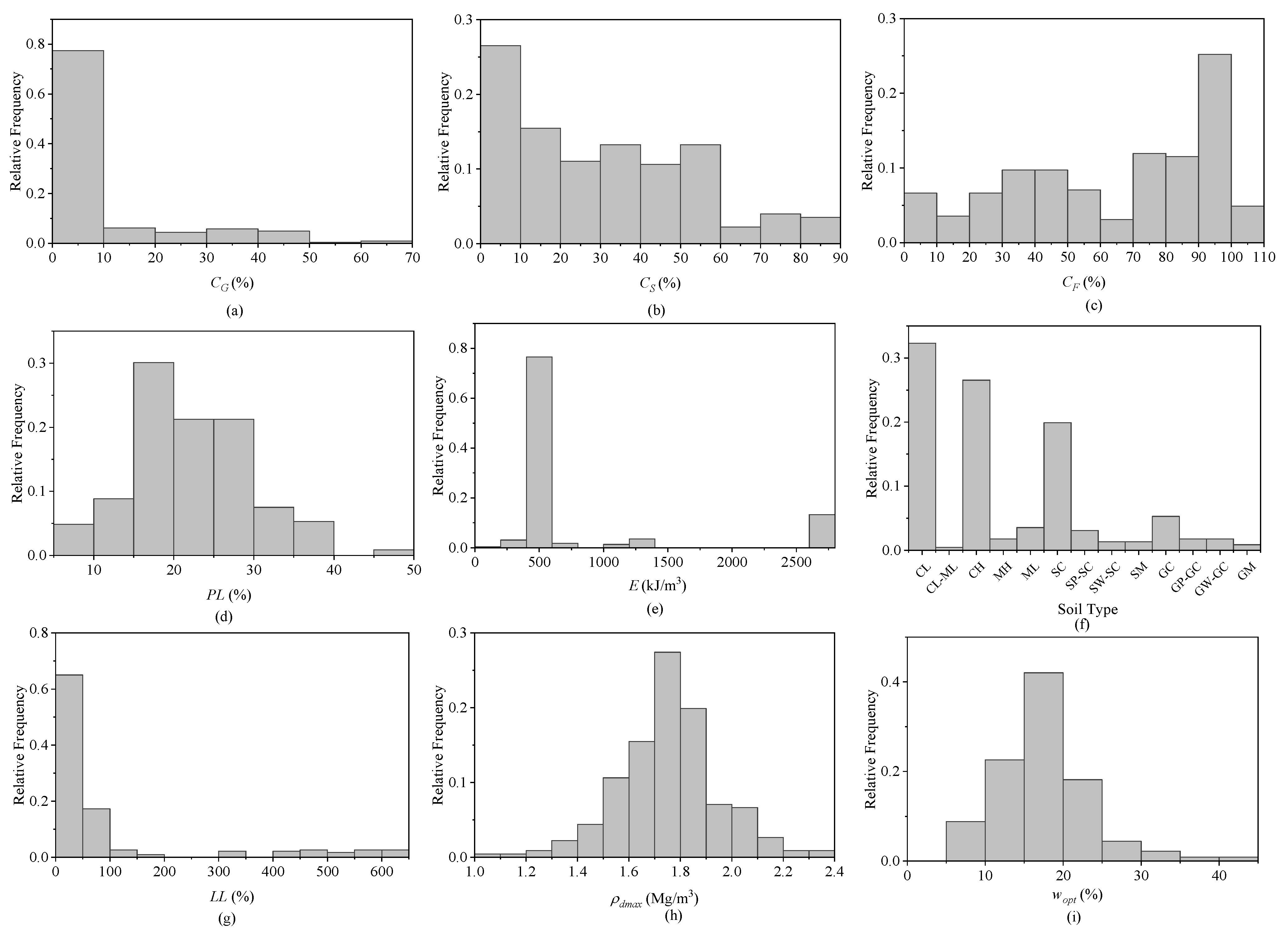
Three error evaluation metrics, namely root mean squared error (RMSE), mean absolute error (MAE), and the coefficient of determination (R2), are chosen to assess the accuracy of MARS model predictions. The R2 metric represents the linear relationship between the predicted and actual values, with its value ranging from zero to one. A value of R2 nearing one signifies a more accurate model prediction. RMSE provides insight into the dispersion between predicted and real data and is sensitive due to its relation to the Euclidean distance. Meanwhile, MAE is a measure of the average magnitude of errors between predicted and observed values. Lower values of RMSE and MAE suggest superior prediction performance by the algorithm. The three metrics are outlined as follows:
Root mean squared error (RMSE):
R M S E = i = 1 n G p i G T i 2 n
Correlation of determination (R2):
R 2 = 1 i = 1 n G p i G T i 2 i = 1 n G T i G T i 2
Mean absolute error (MAE):
M A E = 1 n i = 1 n G p i G T i
where G T i and G p i are the true and predicted values for the observation, respectively. G T i is the mean of all the true values. n is the number of samples.

4. Database Used

In the current research, we utilized data (comprising 226 entries) sourced from the study by [61], which span various soil categories such as fat clay (CH), silty clay (CL-ML), lean clay (CL), clayey gravel (GC), silty gravel (GM), elastic silt (MH), well-graded sand with clay (SW-SC), poorly graded sand with clay (SP-SC), silt (ML), clayey sand (SC), silty sand (SM), poorly graded gravel with clay (GP-GC), and well-graded gravel with clay (GW-GC). The physical attributes of these soil samples are presented in Table 1. This dataset encompasses a diverse array of soils, highlighted by the extensive variety of index properties. Within this dataset, it is posited that the compaction metrics are influenced by factors like liquid limit (LL), plastic limit (PL), compaction energy (E), sand content (CS), fines content (CF), gravel content (CG), optimum water content wopt, and maximum dry density ρdmax, all of which are detailed in Table 1. Figure 4 presents frequency histograms for each variable, inclusive of soil classification. Analyzing Figure 4 reveals that within this database, a significant portion of soils possess gravel and sand contents ranging from 0% to 20% (as seen in Figure 4a,b). Conversely, the content of fines in the soils predominantly falls within 80% to 100% (illustrated in Figure 4c). A large portion of soils register a liquid limit between 0 and 50 (as displayed in Figure 4g), and 32 soils exhibit a liquid limit exceeding 300, indicative of high plasticity. The plastic limit is chiefly found between 10 and 30 (Figure 4d). Notably, this dataset features a comparably larger quantity of clayey sand, fat clay, lean clay, and clayey gravel in contrast to other soil types (depicted in Figure 4f). A significant number of compaction tests were executed under standard Proctor conditions or with diminished compaction energy (not surpassing 600 kJ/m3 as shown in Figure 4e). Around 30 modified Proctor compaction tests are also part of the study. In terms of maximum dry density and optimum water content, peak frequencies are predominantly within 1.6 Mg/m3 to 1.8 Mg/m3 and 10% to 20%, respectively (as captured in Figure 4h,i).

5. Model Results

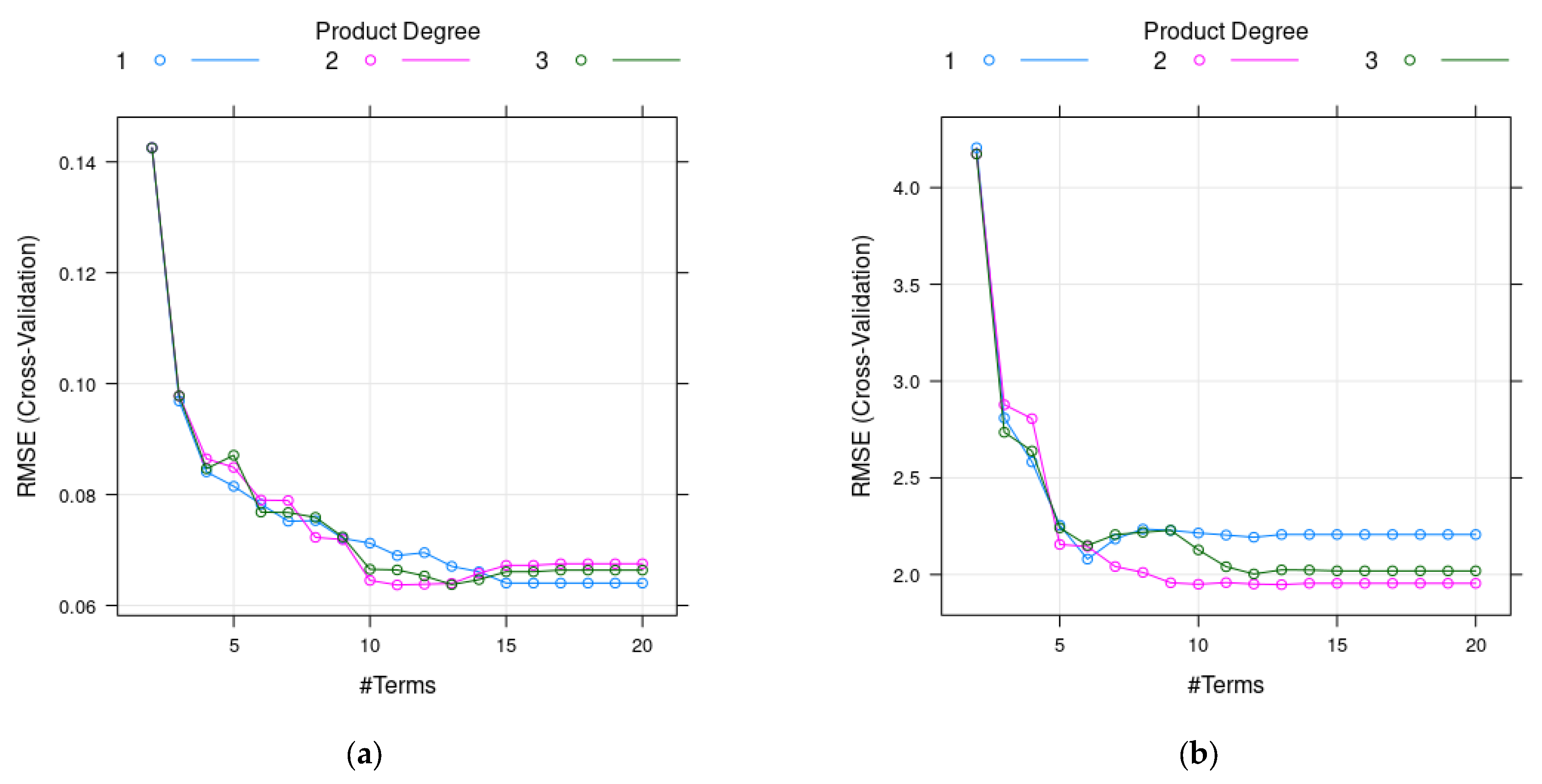
5.1. Hyperparameter Tuning Results for Optimal Model

The hyperparameter tuning procedure, which combined a grid search and k-fold cross-validation, was employed to determine the optimal model parameters for the MARS models, aiming for the lowest RMSE. According to Figure 5, the performance of the MARS model was more sensitive to the ‘nprune’ parameter than the interaction degree, highlighting the crucial role of ‘nprune’ in achieving top-tier model accuracy.
As detailed in Figure 5, a rigorous five-fold cross-validation process pinpointed ‘degree = 2’ and ‘nprune = 13’ as the prime settings for the wopt MARS model. Leveraging these parameters, the model showcased exemplary performance across the 131 training datasets, registering an average RMSE. On the other hand, for the ρdmax MARS model, the most suitable hyperparameters were ‘nprune = 11’ and ‘degree = 2’. With these settings, the model attained an optimal predictive capacity, reflected by an average RMSE of 0.064 and an R2 of 0.889, specifically for predicting the maximum dry density in compacted soil.

5.2. Cross-Validation Results after Hyperparameter Tuning

Post tuning, the performance of the final MARS models was assessed using a five-fold cross-validation procedure. The RMSE, R2, and MAE were computed for each fold to estimate the prediction performance. The results for both models are presented below.
For the wopt model, the five-fold cross-validation results are presented in Table 2:
Table 2. Results derived from a five-fold cross-validation for the wopt model.
FoldsPerformance Measures
RMSE (%)R2MAE (%)
Fold 11.5130.9291.182
Fold 22.3680.8701.867
Fold 31.8270.8861.351
Fold 41.7100.8891.361
Fold 52.3230.8951.728
Average1.9480.8931.498
SD0.3800.0230.287
CoV (%)0.1950.0260.192
Notably, the RMSE, R2, and MAE values indicate the high predictive performance of the MARS model for the wopt parameter, with high R2 values over 0.87 for all folds in both cases. This highlights the models’ ability to capture a significant portion of the variance in the target variables. The RMSE values were relatively low across all folds for both models, underscoring the models’ robustness and their ability to minimize errors in prediction. Moreover, the MAE values were reasonably low, revealing the models’ capability to produce accurate predictions with small deviations from the actual values.
The ρdmax model’s cross-validation results are presented in Table 3.
Once again, the RMSE, R2, and MAE values for each fold reflect the high predictive performance of the model. The average values highlight the overall accuracy of the model, while the standard deviations suggest that the model’s performance is consistent across different folds.
One potential reason some folds perform better than others is due to imbalanced data distribution. If the data are not evenly distributed and one fold ends up with a disproportionate number of certain classes or types of data, the model may perform poorly on that fold. For instance, if one fold contains many outliers or rare events, the model might struggle to generalize. Despite this, the consistently high R2 values, low RMSE and MAE values, and the low standard deviations for both models across all folds underscore the effectiveness of the MARS models and their robustness in predicting the wopt and ρdmax parameters of compacted soil.

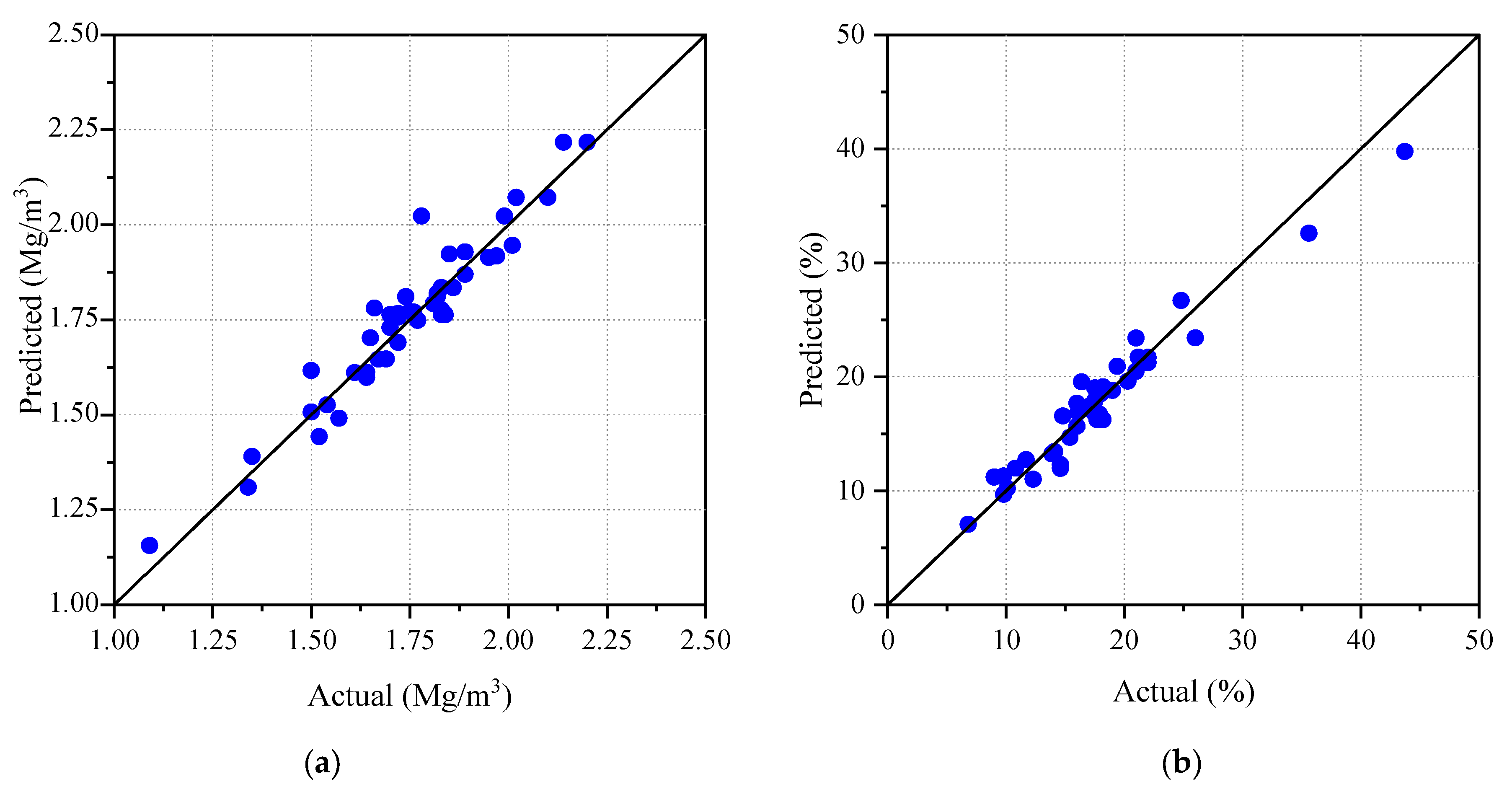
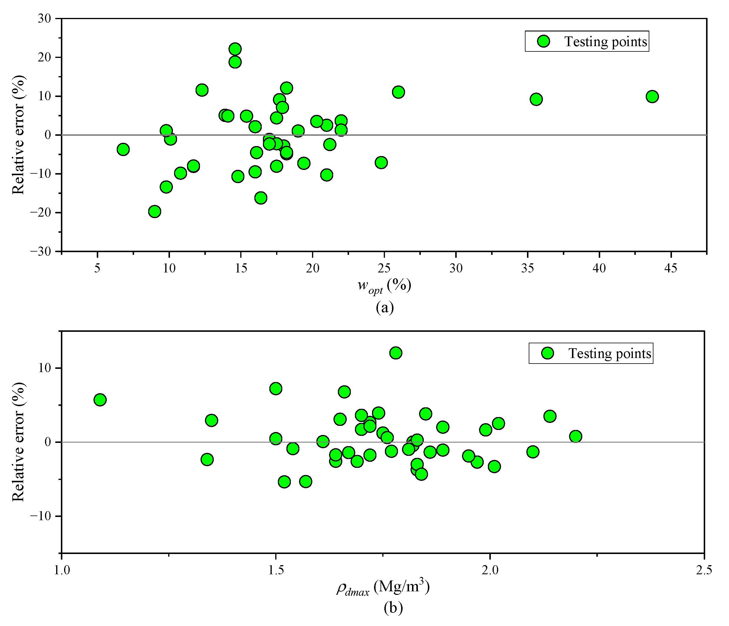
5.3. Evaluation of MARS Models on Unseen Dataset

The following two equations were derived from the final optimal models after hyperparameter tuning for wopt and ρdmax. The equations are as follows:
w o p t = 19.3773983 0.0639987 × m a x ( 97 C F , 0 ) 5.1538333 × m a x ( C F 97,0 ) 0.0898632 × m a x ( 64 L L , 0 ) 0.6415284 × m a x ( 21 P L , 0 ) + 0.4288445 × m a x ( P L 21,0 ) + 0.0025993 × m a x ( 1347 E k J / m 3 , 0 ) + 0.2425873 × m a x ( C F 97,0 ) × P L 0.0000061 × L L × m a x ( E k J / m 3 1347,0 ) + 0.0578447 × m a x ( 7.6 C G , 0 ) × m a x ( 21 P L , 0 ) 0.0093695 × m a x ( 70 C F , 0 ) × m a x ( P L 21,0 ) .
ρ d m a x = 1.39385529 + 0.00261487 × m a x ( 33.1 C S , 0 ) + 0.00621111 × m a x ( 98 C F , 0 ) + 0.00505340 × m a x ( L L 64,0 ) + 0.00337354 × m a x ( 130 L L , 0 ) 0.00526625 × m a x ( L L 130,0 ) 0.01028165 × m a x ( P L 11,0 ) 0.00019175 × m a x ( 1347 E k J / m 3 , 0 ) 0.00188667 × m a x ( C F 98,0 ) × P L 0.00005026 × m a x ( C S 53,0 ) × m a x ( 98 C F , 0 ) + 0.00002616 × m a x ( C F 30,0 ) × m a x ( 130 L L , 0 ) .
The cross plots presented in the subplots (a) and (b) of Figure 6 portray the application of two previous MARS-based models in predicting two crucial parameters for compacted soil: the optimum water content (wopt) and maximum dry density (ρdmax). These subplots showcase the comparison between the models’ predictions and the actual values of wopt and ρdmax for the testing datasets. The plots illustrate that a significant accumulation of data points clustering near the Y = X line signifies the strength and reliability of the established models. Clearly, the implemented models yield predictions that align remarkably well with the unit slope line. As a result, the proposed models can confidently be considered highly reliable for estimating the wopt and ρdmax of compacted soil throughout the testing and training phases.
Figure 7 showcases the relative error of the MARS-based models compared to the actual measurements of wopt and ρdmax. The subplots in Figure 7 demonstrate that the outputs of the proposed MARS-based models exhibit an acceptable deviation from the real measured data. A significant portion of the data falls within the range of −10% to +10% for wopt and −5% to 5% for ρdmax.
Additionally, the statistical evaluation of the proposed models is presented in Table 4, providing a comprehensive summary of the assessment. The table includes the MAE, R2, and RMSE values for the training, testing, and overall datasets. The statistical evaluation clearly indicates that both MARS-based models exhibit outstanding prediction performance. The overall RMSE values for wopt and ρdmax are 1.428 and 0.052, respectively, highlighting the models’ accuracy. The combined findings from Figure 6 and Figure 7, along with the statistical results in Table 4, demonstrate the effectiveness of our newly proposed correlations. They are capable of reliably estimating wopt and ρdmax for compacted soil across various soil properties and operational conditions, showcasing high integrity and efficiency.

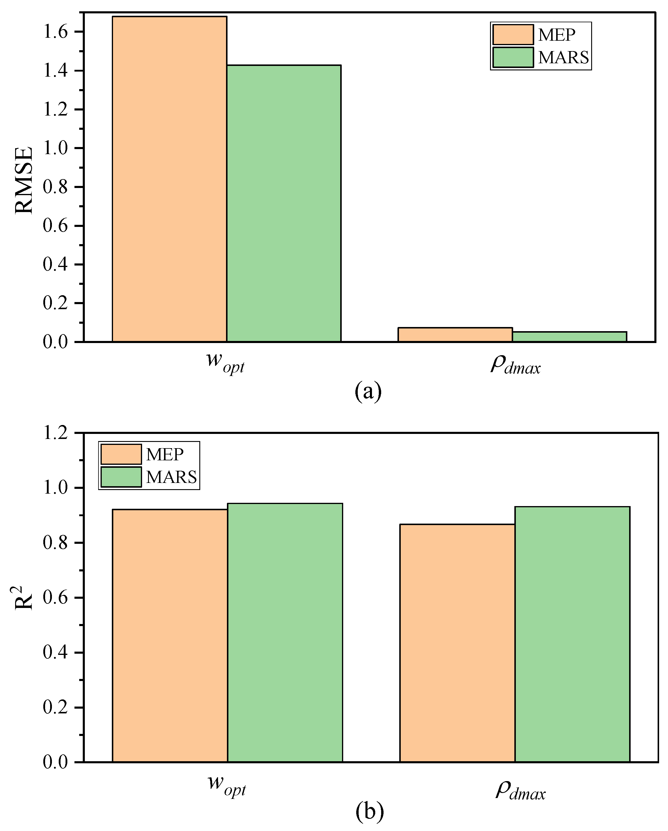
5.4. Comparison between MARS Model with Previously Developed Models

In order to thoroughly assess the reliability of our newly proposed models, we extended the statistical evaluation to compare them with one of the best predictive correlations, namely Multi Expression Programming (MEP) [61]. The comparison is based on various statistical criteria and prediction performance, as presented in Table 5 and visually represented in the bar plots of Figure 8. Analyzing Table 5 and Figure 8 reveals that, despite the satisfactory prediction performance of MEP, our suggested models outperform it in accurately estimating the values of wopt and ρdmax for compacted soil. Furthermore, MEP frequently creates intricate nonlinear empirical models that can be difficult to handle [62]. In turn, the MARS algorithm offers some distinct benefits. Notably, it effectively captures the intricate interactions between independent and dependent variables. Moreover, it eliminates the need to exert extra effort to confirm any preliminary assumptions regarding their relationship. This advantage becomes increasingly vital as the complexity of the problem grows [63].

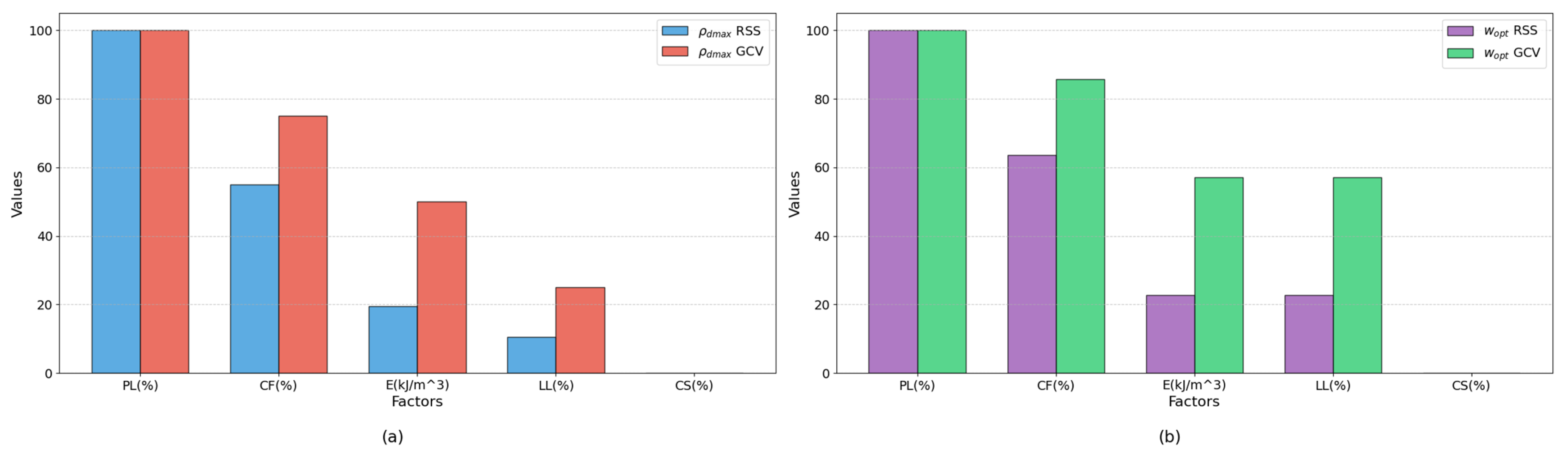
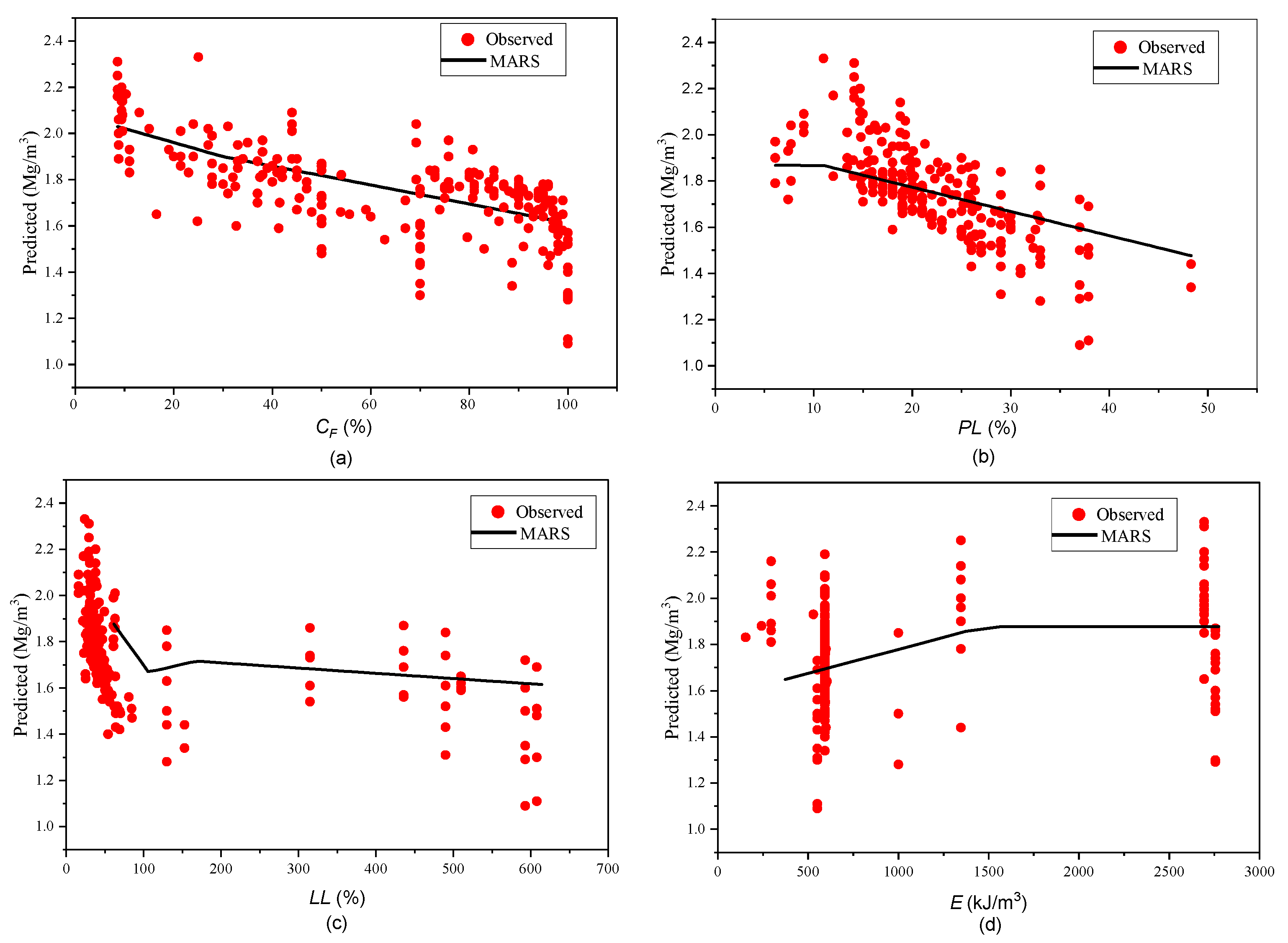
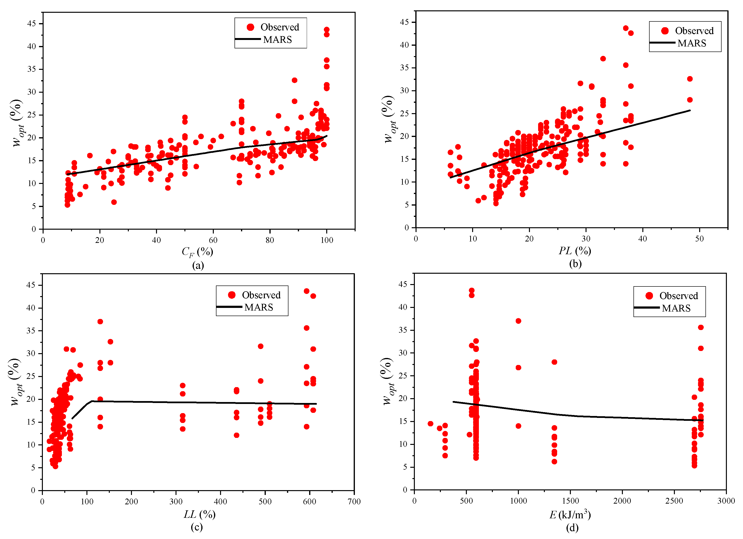
5.5. Variable Importance Analysis

A primary strength of the MARS model is its capability to discern if a particular input factor is vital for predicting output values or if it merely offers a slight enhancement to the model’s precision.
The varImp function in the caret package [64] produces a matrix that displays the relative importance of features within the model, utilizing two distinct methods to assess feature significance:
  • The raw residual sum-of-squares (RSS) method proceeds in two phases. Initially, it assesses the RSS decrease for each subset, contrasting it with the preceding subset’s value. Subsequently, for every relevant feature, it accumulates these reductions across all subsets that incorporate that feature. Finally, the overall sum of these reductions is analyzed. Features leading to substantial RSS declines hold greater importance.
  • The generalized cross-validation (GCV) method operates analogously to the RSS method, but it employs GCV in place of RSS. GCV assesses feature performance in subsets, pinpointing the most pivotal subset (with smaller GCV values being preferable).
Figure 9 displays the outcomes of the contributions and the selections made by different independent variables on the prediction performance of wopt and ρdmax.
Figure 9a displays the impact of various independent variables on the ρdmax MARS model. The figure is sorted based on the decreasing influence of these variables. The top two influential factors are PL (%) and CF (%), with RSS values of 100 and 55.01, and GCV values of 100 and 75, respectively. These statistics suggest that PL (%) holds the most significant influence on the ρdmax MARS model, followed closely by CF (%). Other factors listed in decreasing order of influence are E (kJ/m3), LL (%), and CS (%).
Figure 9b showcases the influence of different independent variables on the wopt MARS model. The two most impactful factors in this table are CF (%) and PL (%). CF (%) takes the lead with RSS and GCV values of 100, indicating its paramount significance in the model. PL (%) follows next with RSS at 63.49 and GCV at 85.71. These results allow us to state that CF (%) has the most considerable influence on the wopt MARS model, but PL (%) also retains significant sway. Other listed factors, in order of influence, include E (kJ/m3), LL (%), and CS (%).
To more deeply assess the reliability of the MARS models, a parametric analysis can be undertaken. This type of analysis examines the alignment of the model’s predictions with existing geotechnical knowledge, experimental data, and anticipated outcomes. This study scrutinized how the predicted soil parameters from the suggested models responded to hypothetical data, spanning the lower and upper bounds of the data used in model training. This approach entailed modifying a single input variable while maintaining others at their average. Synthetic data for this individual parameter were produced via raising it step by step. These inputs were then used in the prediction equation to determine soil parameters. This method was iteratively applied for different variables to gauge the model’s reaction to each input change.
Figure 10 illustrates how the predicted wopt changes in relation to the CF (%), the LL (%), the PL (%), and the E (kJ/m3). Notably, as the CF (%), the LL (%), and the PL (%) rise, the forecasted wopt also goes up. In contrast, when the E (kJ/m3) grows, the predicted value goes down. These consistent changes align with the patterns observed for the wopt in relation to each soil property as seen in the figure, indicating that the proposed model is accurate.
Figure 11 displays the parametric analysis of the anticipated ρdmax in relation to each input variable. Contrary to the wopt, the forecasted ρdmax goes down as the CF (%), LL (%), or PL (%) rises and as the E (kJ/m3) reduces. This trend mirrors the monotonic observations from the actual database illustrated in the figure. Such a parallel between the parametric study and the database in predicting the ρdmax further confirms the accuracy of the model introduced.
The findings from the variable importance analysis are consistent with previously published literature. A respected study explored the influence of CF on the mechanical response of CDG (completely decomposed granite) subjected to dynamic compaction grouting [65]. Through integrating varying proportions of kaolin clay with CDG, this study aimed to understand the implications of fines concentrations on its compactive behavior. The findings indicated that an increment in CF correspondingly results in a diminished ρdmax, while concurrently elevating the wopt. In another study, sand–kaolin blends were compressed to investigate the connection between ρdmax, CF, and specific gravity (Gs) across different moisture levels, with CF ranging from 20% to 70% [66]. A prominent linear correlation (R2 = 0.99) was found between ρdmax and the CF/Gs2 ratio. For PL, a respected paper investigates which index properties best correlate with compaction traits. Incorporating both the study’s findings and the existing literature, it was determined that the plastic limit correlates strongly with compaction features, such as optimum moisture content and maximum dry unit weight, more effectively than either the liquid limit or plasticity index. For the plastic limit (PL), a notable study examined which index properties have the strongest correlation with compaction characteristics [23]. Through integrating the study’s results with the established literature, it was ascertained that the plastic limit shows a significant correlation with compaction attributes, particularly wopt and ρdmax, surpassing the correlations seen with either the liquid limit or the plasticity index.

6. Conclusions

Determining compacted parameters in geotechnical projects is vital for ensuring soil stability, optimizing foundation designs, mitigating settlement issues, and guaranteeing the safety and longevity of structures built on or within the ground. For this reason, the prediction of those parameters is imperative for proactive planning, cost-effective execution, and minimizing project risks. This research aims to predict those parameters via employing the MARS (multivariate adaptive regression splines) model. Compared to other black-box machine learning models, the MARS model offers advantages such as flexibility in capturing non-linear relationships, automated interaction detection, fewer tuning parameters, and the capability to produce more interpretable results, making it particularly suitable for geotechnical applications where understanding the underlying behavior is as crucial as prediction accuracy.
The results obtained through this research indicate the following:
  • Hyperparameter tuning of the MARS model significantly enhanced its predictive performance, reducing the error rate and refining the model’s adaptability to complex geotechnical data.
  • The final optimal models for parameters wopt and ρdmax were evaluated using five-fold cross-validation. The findings showed consistency and high accuracy across all folds, demonstrating the model’s robustness and reliability in estimating these critical parameters.
  • Testing the models on unseen data (testing dataset) revealed that they maintained a commendable level of precision and generalization, further substantiating their efficacy for real-world applications in geotechnical projects.
  • Comparing the MARS model with other state-of-the-art models, such as Multi Expression Programming (MEP), indicated that while both models exhibit strong predictive capabilities, MARS demonstrated faster convergence and better handling of non-linear relationships, offering a more efficient and robust alternative for geotechnical parameter prediction.
  • Finally, the variable importance analysis revealed that the fine content (CF) and plasticity limit (PL) are the most influential factors driving the predictive accuracy of the model, highlighting their pivotal role in determining the geotechnical properties under study.
It is worth mentioning that ML research often presents inherent challenges and limitations. In this study, a notable limitation is the data sample size of 226 points. The model formulated in this research delivers the anticipated accuracy when analogous input parameters are subsequently applied. However, errors may arise in the analysis if the same parameters are used but lie outside our established range. Gathering more experimental data in the future is essential to enhance the model’s generalization capabilities. Upcoming studies will explore the potential of advanced ML techniques, such as deep learning, in predicting wopt and ρdmax values.

Author Contributions

Writing—original draft, H.I.; Investigation, F.J.K.; Software, J.K.A. and M.S.A.; Data curation, S.N.H.; Methodology, F.J.K.; Supervision, M.S.A.; Funding acquisition, L.F.A.B.; Validation, J.K.A.; Writing—review and editing, H.I. and L.F.A.B. All authors have read and agreed to the published version of the manuscript.

Funding

This research received no external funding.

Institutional Review Board Statement

Not applicable.

Informed Consent Statement

Not applicable.

Data Availability Statement

Not applicable.

Conflicts of Interest

The authors declare no conflict of interest.

References

  1. Verma, G.; Kumar, B. Prediction of compaction parameters for fine-grained and coarse-grained soils: A review. Int. J. Geotech. Eng. 2020, 14, 970–977. [Google Scholar] [CrossRef]
  2. Proctor, R. Fundamental principles of soil compaction. Eng. News-Rec. 1933, 111, 245–248, 286–289, 348–351. [Google Scholar]
  3. Hussain, A.; Atalar, C. Estimation of compaction characteristics of soils using Atterberg limits. Proc. IOP Conf. Ser. Mater. Sci. Eng. 2020, 800, 012024. [Google Scholar] [CrossRef]
  4. Rimbarngaye, A.; Mwero, J.N.; Ronoh, E.K. Effect of gum Arabic content on maximum dry density and optimum moisture content of laterite soil. Heliyon 2022, 8, e11553. [Google Scholar] [CrossRef]
  5. Spagnoli, G.; Shimobe, S. An overview on the compaction characteristics of soils by laboratory tests. Eng. Geol. 2020, 278, 105830. [Google Scholar] [CrossRef]
  6. Ren, X.-C.; Lai, Y.-M.; Zhang, F.-Y.; Hu, K. Test method for determination of optimum moisture content of soil and maximum dry density. KSCE J. Civ. Eng. 2015, 19, 2061–2066. [Google Scholar] [CrossRef]
  7. Lim, Y.Y.; Miller, G.A. Wetting-induced compression of compacted Oklahoma soils. J. Geotech. Geoenviron. Eng. 2004, 130, 1014–1023. [Google Scholar] [CrossRef]
  8. Delage, P.; Marcial, D.; Cui, Y.; Ruiz, X. Ageing effects in a compacted bentonite: A microstructure approach. Géotechnique 2006, 56, 291–304. [Google Scholar] [CrossRef]
  9. Rahman, F.; Hossain, M.; Hunt, M.; Romanoschi, S. Soil stiffness evaluation for compaction control of cohesionless embankments. Geotech. Test. J. 2008, 31, 442–451. [Google Scholar]
  10. Di Matteo, L.; Bigotti, F.; Ricco, R. Best-fit models to estimate modified proctor properties of compacted soil. J. Geotech. Geoenviron. Eng. 2009, 135, 992–996. [Google Scholar] [CrossRef]
  11. Sun, D.a.; Cui, H.; Sun, W. Swelling of compacted sand–bentonite mixtures. Appl. Clay Sci. 2009, 43, 485–492. [Google Scholar] [CrossRef]
  12. Zhao, L.-S.; Zhou, W.-H.; Yuen, K.-V. A simplified axisymmetric model for column supported embankment systems. Comput. Geotech. 2017, 92, 96–107. [Google Scholar] [CrossRef]
  13. Chen, R.-P.; Wang, H.-L.; Hong, P.-Y.; Cui, Y.-J.; Qi, S.; Cheng, W. Effects of degree of compaction and fines content of the subgrade bottom layer on moisture migration in the substructure of high-speed railways. Proc. Inst. Mech. Eng. Part F J. Rail Rapid Transit 2018, 232, 1197–1210. [Google Scholar] [CrossRef]
  14. Chen, R.-P.; Qi, S.; Wang, H.-L.; Cui, Y.-J. Microstructure and hydraulic properties of coarse-grained subgrade soil used in high-speed railway at various compaction degrees. J. Mater. Civ. Eng. 2019, 31, 04019301. [Google Scholar] [CrossRef]
  15. Ardakani, A.; Kordnaeij, A. Soil compaction parameters prediction using GMDH-type neural network and genetic algorithm. Eur. J. Environ. Civ. Eng. 2019, 23, 449–462. [Google Scholar] [CrossRef]
  16. Wang, H.-L.; Chen, R.-P. Estimating static and dynamic stresses in geosynthetic-reinforced pile-supported track-bed under train moving loads. J. Geotech. Geoenviron. Eng. 2019, 145, 04019029. [Google Scholar] [CrossRef]
  17. Benbouras, M.A.; Lefilef, L. Progressive machine learning approaches for predicting the soil compaction parameters. Transp. Infrastruct. Geotechnol. 2023, 10, 211–238. [Google Scholar] [CrossRef]
  18. ASTM D698; Standard Test Methods for Laboratory Compaction Characteristics of Soil Using Standard Effort (12,400 ft-lbf/ft3 (600 kN-m/m3)). ASTM International: West Conshohocken, PA, USA, 2021; p. 13.
  19. ASTM D1557; Standard Test Methods for Laboratory Compaction Characteristics of Soil Using Modiefied Effort (56,000 ft-lbf/ft3 (2,700 kN-m/m3)). ASTM International: West Conshohocken, PA, USA, 2021; pp. 1–10.
  20. Blotz, L.R.; Benson, C.H.; Boutwell, G.P. Estimating optimum water content and maximum dry unit weight for compacted clays. J. Geotech. Geoenviron. Eng. 1998, 124, 907–912. [Google Scholar] [CrossRef]
  21. Omar, M.; Shanableh, A.; Basma, A.; Barakat, S. Compaction characteristics of granular soils in United Arab Emirates. Geotech. Geol. Eng. 2003, 21, 283–295. [Google Scholar] [CrossRef]
  22. Gurtug, Y.; Sridharan, A. Compaction behaviour and prediction of its characteristics of fine grained soils with particular reference to compaction energy. Soils Found. 2004, 44, 27–36. [Google Scholar] [CrossRef]
  23. Sridharan, A.; Nagaraj, H. Plastic limit and compaction characteristics of finegrained soils. Proc. Inst. Civ. Eng. Ground Improv. 2005, 9, 17–22. [Google Scholar] [CrossRef]
  24. Mujtaba, H.; Farooq, K.; Sivakugan, N.; Das, B.M. Correlation between gradational parameters and compaction characteristics of sandy soils. Int. J. Geotech. Eng. 2013, 7, 395–401. [Google Scholar] [CrossRef]
  25. Farooq, K.; Khalid, U.; Mujtaba, H. Prediction of compaction characteristics of fine-grained soils using consistency limits. Arab. J. Sci. Eng. 2016, 41, 1319–1328. [Google Scholar] [CrossRef]
  26. Taha, O.M.E.; Majeed, Z.H.; Ahmed, S.M. Artificial neural network prediction models for maximum dry density and optimum moisture content of stabilized soils. Transp. Infrastruct. Geotechnol. 2018, 5, 146–168. [Google Scholar] [CrossRef]
  27. Othman, K.; Abdelwahab, H. Prediction of the soil compaction parameters using deep neural networks. Transp. Infrastruct. Geotechnol. 2021, 10, 147–164. [Google Scholar] [CrossRef]
  28. Verma, G.; Kumar, B. Multi-layer perceptron (MLP) neural network for predicting the modified compaction parameters of coarse-grained and fine-grained soils. Innov. Infrastruct. Solut. 2022, 7, 78. [Google Scholar] [CrossRef]
  29. Bardhan, A.; Singh, R.K.; Ghani, S.; Konstantakatos, G.; Asteris, P.G. Modelling Soil Compaction Parameters Using an Enhanced Hybrid Intelligence Paradigm of ANFIS and Improved Grey Wolf Optimiser. Mathematics 2023, 11, 3064. [Google Scholar] [CrossRef]
  30. Verma, G.; Kumar, B. Artificial neural network equations for predicting the modified proctor compaction parameters of fine-grained soil. Transp. Infrastruct. Geotechnol. 2023, 10, 424–447. [Google Scholar] [CrossRef]
  31. Hasnat, A.; Hasan, M.M.; Islam, M.R.; Alim, M.A. Prediction of compaction parameters of soil using support vector regression. Curr. Trends Civ. Struct. Eng. 2019, 4, 1–7. [Google Scholar] [CrossRef]
  32. Ferreira, C. Gene expression programming: A new adaptive algorithm for solving problems. arXiv 2001, arXiv:pcs/0102027. [Google Scholar]
  33. Raja, M.N.A.; Abdoun, T.; El-Sekelly, W. Smart prediction of liquefaction-induced lateral spreading. J. Rock Mech. Geotech. Eng. 2023. [Google Scholar] [CrossRef]
  34. Jalal, F.E.; Xu, Y.; Iqbal, M.; Jamhiri, B.; Javed, M.F. Predicting the compaction characteristics of expansive soils using two genetic programming-based algorithms. Transp. Geotech. 2021, 30, 100608. [Google Scholar] [CrossRef]
  35. Jalal, F.E.; Iqbal, M.; Ali Khan, M.; Salami, B.A.; Ullah, S.; Khan, H.; Nabil, M. Indirect estimation of swelling pressure of expansive soil: Gep versus mep modelling. Adv. Mater. Sci. Eng. 2023, 2023, 1827117. [Google Scholar] [CrossRef]
  36. Samui, P. Determination of ultimate capacity of driven piles in cohesionless soil: A multivariate adaptive regression spline approach. Int. J. Numer. Anal. Methods Geomech. 2012, 36, 1434–1439. [Google Scholar] [CrossRef]
  37. Samui, P. Multivariate adaptive regression spline (Mars) for prediction of elastic modulus of jointed rock mass. Geotech. Geol. Eng. 2013, 31, 249–253. [Google Scholar] [CrossRef]
  38. Deng, Z.-P.; Pan, M.; Niu, J.-T.; Jiang, S.-H.; Qian, W.-W. Slope reliability analysis in spatially variable soils using sliced inverse regression-based multivariate adaptive regression spline. Bull. Eng. Geol. Environ. 2021, 80, 7213–7226. [Google Scholar] [CrossRef]
  39. Ghanizadeh, A.R.; Rahrovan, M. Modeling of unconfined compressive strength of soil-RAP blend stabilized with Portland cement using multivariate adaptive regression spline. Front. Struct. Civ. Eng. 2019, 13, 787–799. [Google Scholar] [CrossRef]
  40. Zheng, G.; Zhang, W.; Zhou, H.; Yang, P. Multivariate adaptive regression splines model for prediction of the liquefaction-induced settlement of shallow foundations. Soil Dyn. Earthq. Eng. 2020, 132, 106097. [Google Scholar] [CrossRef]
  41. Zuo, Q. Settlement prediction of the piles socketed into rock using multivariate adaptive regression splines. J. Appl. Sci. Eng. 2022, 26, 111–119. [Google Scholar]
  42. Sirimontree, S.; Jearsiripongkul, T.; Lai, V.Q.; Eskandarinejad, A.; Lawongkerd, J.; Seehavong, S.; Thongchom, C.; Nuaklong, P.; Keawsawasvong, S. Prediction of penetration resistance of a spherical penetrometer in clay using multivariate adaptive regression splines model. Sustainability 2022, 14, 3222. [Google Scholar] [CrossRef]
  43. Emamgolizadeh, S.; Bateni, S.; Shahsavani, D.; Ashrafi, T.; Ghorbani, H. Estimation of soil cation exchange capacity using genetic expression programming (GEP) and multivariate adaptive regression splines (MARS). J. Hydrol. 2015, 529, 1590–1600. [Google Scholar] [CrossRef]
  44. Haghiabi, A.H. Prediction of river pipeline scour depth using multivariate adaptive regression splines. J. Pipeline Syst. Eng. Pract. 2017, 8, 04016015. [Google Scholar] [CrossRef]
  45. Conoscenti, C.; Ciaccio, M.; Caraballo-Arias, N.A.; Gómez-Gutiérrez, Á.; Rotigliano, E.; Agnesi, V. Assessment of susceptibility to earth-flow landslide using logistic regression and multivariate adaptive regression splines: A case of the Belice River basin (western Sicily, Italy). Geomorphology 2015, 242, 49–64. [Google Scholar] [CrossRef]
  46. Sharda, V.; Prasher, S.; Patel, R.; Ojasvi, P.; Prakash, C. Performance of Multivariate Adaptive Regression Splines (MARS) in predicting runoff in mid-Himalayan micro-watersheds with limited data/Performances de régressions par splines multiples et adaptives (MARS) pour la prévision d’écoulement au sein de micro-bassins versants Himalayens d’altitudes intermédiaires avec peu de données. Hydrol. Sci. J. 2008, 53, 1165–1175. [Google Scholar]
  47. R Core Team. R: A Language and Environment for Statistical Computing; R Core Team: Vienna, Austria, 2020. [Google Scholar]
  48. Friedman, J.H. Multivariate adaptive regression splines. Ann. Stat. 1991, 19, 1–67. [Google Scholar] [CrossRef]
  49. Loh, W.Y. Classification and regression trees. Data Min. Knowl. Discov. 2011, 1, 14–23. [Google Scholar] [CrossRef]
  50. Kuhn, M.; Johnson, K. Applied Predictive Modeling; Springer: Berlin/Heidelberg, Germany, 2013; Volume 26. [Google Scholar]
  51. Alhakeem, Z.M.; Jebur, Y.M.; Henedy, S.N.; Imran, H.; Bernardo, L.F.; Hussein, H.M. Prediction of ecofriendly concrete compressive strength using gradient boosting regression tree combined with GridSearchCV hyperparameter-optimization techniques. Materials 2022, 15, 7432. [Google Scholar] [CrossRef] [PubMed]
  52. Yang, Z.; Gao, W.; Chen, L.; Yuan, C.; Chen, Q.; Kong, Q. A novel electromechanical impedance-based method for non-destructive evaluation of concrete fiber content. Constr. Build. Mater. 2022, 351, 128972. [Google Scholar] [CrossRef]
  53. Koya, B.P.; Aneja, S.; Gupta, R.; Valeo, C. Comparative analysis of different machine learning algorithms to predict mechanical properties of concrete. Mech. Adv. Mater. Struct. 2022, 29, 4032–4043. [Google Scholar] [CrossRef]
  54. Tang, F.; Wu, Y.; Zhou, Y. Hybridizing grid search and support vector regression to predict the compressive strength of fly ash concrete. Adv. Civ. Eng. 2022, 2022, 3601914. [Google Scholar] [CrossRef]
  55. Luo, H.; Paal, S.G. Machine learning–based backbone curve model of reinforced concrete columns subjected to cyclic loading reversals. J. Comput. Civ. Eng. 2018, 32, 04018042. [Google Scholar] [CrossRef]
  56. Rodriguez, J.D.; Perez, A.; Lozano, J.A. Sensitivity analysis of k-fold cross validation in prediction error estimation. IEEE Trans. Pattern Anal. Mach. Intell. 2009, 32, 569–575. [Google Scholar] [CrossRef]
  57. Kohavi, R. A study of cross-validation and bootstrap for accuracy estimation and model selection. In Proceedings of the 14th International Joint Conference on Artificial Intelligence (IJCAI), Montreal, QC, Canada, 20 August 1995; Volume 14, pp. 1137–1145. [Google Scholar]
  58. Wong, T.-T. Performance evaluation of classification algorithms by k-fold and leave-one-out cross validation. Pattern Recognit. 2015, 48, 2839–2846. [Google Scholar] [CrossRef]
  59. Liu, X.; Liu, T.; Feng, P. Long-term performance prediction framework based on XGBoost decision tree for pultruded FRP composites exposed to water, humidity and alkaline solution. Compos. Struct. 2022, 284, 115184. [Google Scholar] [CrossRef]
  60. Hastie, T.; Tibshirani, R.; Friedman, J.H.; Friedman, J.H. The Elements of Statistical Learning: Data Mining, Inference, and prediction; Springer: Cham, Switzerland, 2009; Volume 2. [Google Scholar]
  61. Wang, H.-L.; Yin, Z.-Y. High performance prediction of soil compaction parameters using multi expression programming. Eng. Geol. 2020, 276, 105758. [Google Scholar] [CrossRef]
  62. Shah, H.A.; Nehdi, M.L.; Khan, M.I.; Akmal, U.; Alabduljabbar, H.; Mohamed, A.; Sheraz, M. Predicting Compressive and Splitting Tensile Strengths of Silica Fume Concrete Using M5P Model Tree Algorithm. Materials 2022, 15, 5436. [Google Scholar] [CrossRef]
  63. Kaveh, A.; Bakhshpoori, T.; Hamze-Ziabari, S. New model derivation for the bond behavior of NSM FRP systems in concrete. Iran. J. Sci. Technol. Trans. Civ. Eng. 2017, 41, 249–262. [Google Scholar] [CrossRef]
  64. Kuhn, M. Building predictive models in R using the caret package. J. Stat. Softw. 2008, 28, 1–26. [Google Scholar] [CrossRef]
  65. Wang, S.; Chan, D.; Lam, K.C. Experimental study of the effect of fines content on dynamic compaction grouting in completely decomposed granite of Hong Kong. Constr. Build. Mater. 2009, 23, 1249–1264. [Google Scholar] [CrossRef]
  66. Alshameri, B. Maximum dry density of sand–kaolin mixtures predicted by using fine content and specific gravity. SN Appl. Sci. 2020, 2, 1693. [Google Scholar] [CrossRef]
Figure 1. Research methodology.
Applsci 13 11634 g001
Figure 2. Graph representing two splines associated with the variable x: the left spline, represented by a dashed line (for x less than t, the formula is −(xt)), and the right spline, represented by a solid black line (for x greater than t, the formula is +(xt)).
Applsci 13 11634 g002
Figure 3. Tuning of hyperparameters using five-fold cross-validation.
Applsci 13 11634 g003
Figure 4. Relative frequency distribution of input and output variables.
Applsci 13 11634 g004
Figure 5. Optimization results of hyperparameter tuning for the MARS models: (a) ρdmax and (b) wopt.
Applsci 13 11634 g005
Figure 6. Actual vs. predicted values using the MARS model for the testing dataset: (a) ρdmax and (b) wopt.
Applsci 13 11634 g006
Figure 7. Comparison of relative errors vs. real value: (a) MARS-based model for wopt; (b) MARS-based model for ρdmax.
Applsci 13 11634 g007
Figure 8. Comparative performance of MARS vs. MEP models: (a) RMSE; (b) R2.
Applsci 13 11634 g008
Figure 9. Influence of different independent variables on MARS model: (a) for ρdmax; (b) for wopt.
Applsci 13 11634 g009
Figure 10. Parametric analysis of the predicted wopt versus: (a) CF (%); (b) PL (%); (c) LL (%); (d) E (kJ/m3).
Applsci 13 11634 g010
Figure 11. Parametric analysis of the predicted wopt versus: (a) CF (%); (b) PL (%); (c) LL (%); (d) E (kJ/m3).
Applsci 13 11634 g011
Table 1. Model variable descriptive statistics.
StatisticsCG (%)CS (%)CF (%)LL (%)PL (%)E (kJ/m3)wopt (%)ρdmax (Mg/m3)
Standard deviation14.56623.38830.016164.2187.405735.4355.9640.199
Mean7.46829.44863.088108.72722.005894.06617.5121.751
Median0.00027.00070.00040.65020.150593.00017.0001.750
Maximum67.10089.000100.000608.00048.3002755.00043.7002.330
Minimum0.0000.0008.60016.0006.100155.0005.3001.090
Kurtosis3.482−0.471−1.2503.2640.7482.2662.8620.977
Table 3. Results derived from a five-fold cross-validation for the ρdmax model.
FoldsPerformance Measures
RMSE (Mg/m3)R2MAE (Mg/m3)
Fold 10.0680.8600.051
Fold 20.0670.9080.050
Fold 30.0480.9480.040
Fold 40.0710.8700.057
Fold 50.0650.9090.049
Average0.0640.8990.050
SD0.0090.0350.006
CoV (%)0.1410.0390.120
Table 4. Performance metrics of the MARS models for training, testing, and overall datasets.
TrainingTestingOverall
woptMAE (%)1.121.2761.15
RMSE (%)1.3921.5771.428
R20.9420.9480.943
ρdmaxMAE (Mg/m3)0.040.0470.041
RMSE (Mg/m3)0.050.0620.052
R20.9360.9190.931
Table 5. Performance metrics of the MEP models for training, testing, and overall datasets.
Compaction ParametersPerformance MeasuresOverall
woptMAE (%)1.3
RMSE (%)1.68
R20.921
ρdmaxMAE (Mg/m3)0.054
RMSE (Mg/m3)0.073
R20.867
Disclaimer/Publisher’s Note: The statements, opinions and data contained in all publications are solely those of the individual author(s) and contributor(s) and not of MDPI and/or the editor(s). MDPI and/or the editor(s) disclaim responsibility for any injury to people or property resulting from any ideas, methods, instructions or products referred to in the content.

