Receding Horizon Optimization for Cooperation of Connected Vehicles at Signal-Free Intersections under Mixed-Automated Traffic

Abstract

This paper proposes a distributed coordination scheme for connected vehicles, including automated vehicles (AVs) and manual vehicles (MVs), at signal-free intersections. The cooperation issue of vehicles at an intersection is formulated into a multi-objective optimization problem that aims to eliminate conflicts and improve traffic mobility and fuel economy. For this purpose, the future trajectories of AVs and MVs are predicted by the respective car-following models, and are shared with neighboring vehicles in conflict relationships. The proposed scheme optimizes the sum of the performance of AVs within the cooperative zone in a prediction horizon. A distributed optimization algorithm in the receding horizon is presented to obtain the local optimal solutions, and is tested in simulations with different demand levels and penetration rates of AVs. The results show that the proposed scheme reduces travel time by 29.7–45.5% and 34.5–49.2%, and decreases fuel consumption by 27.6–35.3% and 21.6–29.9% under 70–100% penetration rates of AVs, compared to the no-control operation and fixed-time signal control strategy. In addition, a comparison simulation with the strategy of jointly optimizing the vehicle trajectory and signal timing is conducted to evaluate the relative merits of the proposed scheme.

1. Introduction

1.1. Background

Social progress and improvements in people’s quality of life profit from the rapid development of urban transportation. Unfortunately, a sharp increase in vehicle ownership poses great challenges in traffic safety, mobility, and environmental sustainability [1]. Over the decades, the development of intelligent transportation systems (ITSs) has become a significant force in dealing with these challenges. In particular, emerging connected vehicles (CVs) technologies have aroused widespread attention due to their enormous potential in improving road capacity, driving safety, and fuel economy. Employing vehicle-to-everything (V2X) communication, CVs are able to cooperate in various traffic scenarios [2].

As bottlenecks of urban traffic, intersections have always been the focus of researchers and traffic engineers for improving traffic safety and smoothing traffic flow. Intersections can be categorized into two types, i.e., signalized and signal-free. Researchers have proposed various approaches to improve traffic efficiency at signalized intersections, e.g., fixed-time control, actuated control, adaptive control, and connected-vehicle-based methods [3,4]. These methods can improve traffic throughput at intersections to some extent, but unnecessary stopping and idling are still inevitable. For signal-free intersections, there are no signal lights or any other display devices to prompt drivers. Traditionally, drivers must observe and estimate the adequate vehicle clearance through visual judgment for safe crossing. Currently, a real-time and reliable CVs environment can be constructed using the V2X communication technology, which provides faster response and shorter vehicular gaps for AVs to pass through intersections. Significant efforts have been made to coordinate AVs at signal-free intersections under centralized or decentralized frameworks. The centralized frameworks globally decide the movements of all vehicles using a central controller, while under the decentralized frameworks, each vehicle is treated as a single agent and collaborates independently [5]. Two kinds of strategies have generally been presented for signal-free intersection coordination under the centralized or decentralized frameworks, i.e., heuristic strategies and trajectory planning strategies.

1.2. Literature Review

Heuristic strategies aim at adjusting the movements of vehicles to cross an intersection without collisions; they generally adopt the rule of first come, first served (FCFS). Typical heuristic strategies that have been proposed in the literature include resource reservation [6,7], fuzzy logic [8,9], and virtual platooning [10,11]. For instance, Dresner et al. [6] proposed a centralized resource reservation method to coordinate vehicles at a signal-free intersection with a single straight lane in each direction. This work was further extended in [7], which considered turning and improved the performance of the central controller. The central controller frequently interacted with vehicles and scheduled the time slots and space tiles, which suffered heavy communication burdens and the risk of deadlocks. Note that the existing heuristic strategies only regulate vehicles to pass through intersections without conflicts, but are incapable of further optimizing the trajectories of vehicles. In addition to collision avoidance, the trajectory planning strategies drive vehicles to a better traffic performance. For example, Lee et al. [12] presented a trajectory optimization algorithm to minimize the length of potential conflicting overlapping trajectories. Considering vehicle jitter, acceleration, and expected velocity, Dai et al. [13] formulated a multi-objective trajectory optimization problem. By using a Monte Carlo tree search, Xu et al. [14] planned the trajectories of vehicles through the global-optimal passing orders. Planning-based strategies have been shown to perform better than heuristic strategies under high traffic demand [15]. However, the trajectory planning strategies have a weakness in real-time practical implementation since the computation of the formulated problems suffers the curse of dimensionality.

Several recent studies on the cooperation of vehicles at signal-free intersections introduced the concept of multi-agent, i.e., consensus, control [16,17]. The coordinated vehicles are regulated to approach a desired state of motion to avoid collisions at intersections. For instance, Mirheli et al. [18] proposed a coordinated optimization trajectory algorithm by formulating a mixed-integer non-linear program (MILP), which aims at forcing vehicles to reach consensus. This approach pushed the distributed vehicle-level solutions toward global optimality, but the formulated MILP problems suffered a heavy computational burden. Xu et al. [11] presented a virtual consensus-based platoon control approach by transforming the two-dimensional vehicle cluster at the intersection into a one-dimensional virtual platoon in a virtual lane. However, this approach was not evaluated in the receding horizon framework. For those problems of vehicle collaboration at signal-free intersections, receding horizon control (RHC), also known as model predictive control (MPC) [19], has been utilized to dynamically capture predictions on vehicle states and future trajectories to optimize the coordination systems in real time. In the vehicle–intersection coordination framework proposed in [20], a conflict risk indicator was integrated into the MPC controller. Du et al. [21] formulated the corridor-level vehicle coordination problem in the RHC framework, where vehicle collision was avoided by using a consensus algorithm to force vehicles to track the reference speed.

Note that the existing research on the cooperation of vehicles at signal-free intersections is only confined to the fully connected AV environment. Since the mixed driving environment containing AVs and MVs will stay with us for an extended period, it is essential to establish control mechanisms for cooperating with both types of vehicles. In the current study, traffic signal lights still have to be used to regulate the mixed autonomy traffic flow at intersections [22,23]. To jointly optimize the signal timing and vehicle trajectories, a complex MILP is constructed [24]. However, MILP problems are NP-hard, in which the computational burden grows exponentially with the number of loading vehicles [25]. Moreover, introducing traffic lights still inevitably leads to stops and idling. Furthermore, some of the existing collision avoidance algorithms at signal-free intersections can only deal with the problems with just a few vehicles due to computation complexity [21,26]. The presented algorithms cannot be applied in a realistic traffic environment to coordinate vehicles globally under a receding horizon framework. In addition, the centralized coordination approaches suffer heavy computational burdens and struggle to handle high-density traffic. Whereas distributed coordination frameworks have the advantages of a lower communication burden, lower computational complexity, and better information protection. Nevertheless, the existing approaches on the distributed coordination of AVs at signal-free intersections are inadequate in some respects, e.g., a lack of restrictions on control inputs, vehicle states, and safety conditions [11], without fully considering the global conflict relationships [26,27], and losing sight of the mixed-automated vehicles environment [11,18,21,26,28]. To address the problem of the cooperation of AVs and MVs at signal-free intersections, we establish a distributed collaboration framework to address the above issues.

1.3. Contribution of This Work

In this paper, we develop a distributed cooperation scheme to coordinate AVs and MVs to pass through signal-free intersections. The core idea is to cooperatively regulate each AV to cross the intersection while keeping a safe distance with the vehicles in conflict relationships. Firstly, a conflict graph is constructed to describe the conflict relationships of the different approaching lanes. Based on the conflict graph, the communication topologies of vehicles are identified in real time. Then, the future trajectories of AVs and MVs are predicted by the respective car-following models and are shared with their neighboring vehicles in conflict relationships. By utilizing the predicted trajectory information of the conflicting MVs, AVs proactively optimize their trajectories to avoid conflicts while assisting the MVs to cross the intersection smoothly. In addition, the elimination of conflicts, traffic mobility, and fuel economy are synchronously considered in the proposed scheme. The intersection coordination issue is formulated into a multi-objective optimization problem aiming to minimize the weighted performance indexes of AVs in a prediction period. Finally, a receding horizon optimization algorithm is presented and tested with a typical four-phase intersection in simulations. The contributions of this study are listed below:

(1)

Different from the existing literature only considering coordinating vehicles under a fully AV environment, this paper proposes a coordination scheme under which AVs and MVs can cooperatively pass through a signal-free intersection;

(2)

The proposed scheme develops a practical application which concurrently considers the restrictions of control inputs, vehicle states, safety conditions, global conflict relationships, and the mixed-automated driving environment;

(3)

A distributed multi-objective optimization algorithm is presented to synchronously eliminate the traffic conflicts and improve mobility and fuel economy in a receding horizon framework.

The remainder of this paper is structured as follows. Section 2 describes the problem statement. Section 3 details the methodology to formulate and solve the cooperative control problem and gives the receding horizon optimization algorithm. Simulations are conducted in Section 4; and Section 5 concludes this paper.

2. Problem Statement

We consider a typical symmetrical dual-lane intersection with four approaches and departures, as depicted in Figure 1. Each approach consists of a straight lane and a left-turn lane. Right-turn lanes are omitted here for simplicity since they have no impact on the collaboration results of the intersection. Here, we define a cooperative zone (CZ) with the scope of the four approaching lanes under the radius R. An intersection coordination unit (ICU) deployed in the center of the intersection assists the vehicles in sharing information in the CZ.

We assume that all vehicles are connected, and equipped with GPS or BDS, vehicle-to-infrastructure (V2I), and vehicle-to-vehicle (V2V) communication devices to exchange real-time information with the ICU and other vehicles. Each vehicle in the CZ transmits four necessary properties to the ICU, i.e., vehicle ID, vehicle type, origin-destination, and vehicle state (position and speed). (1) A vehicle ID will be automatically assigned to the vehicle when entering the CZ; (2) There are two vehicle types considered in this study: AVs and MVs. We consider high penetration rates of AVs (no less than 70%) in this paper to decrease traffic insecurity factors and alleviate drops in traffic efficiency caused by MVs; (3) The origin–destination of a vehicle means which edges the vehicle enters and departs from in the road network; (4) The vehicle state is the crucial information used to predict the future trajectory of the vehicle, which is transmitted to the correlative neighboring vehicles. At each time step, the ICU receives the information of the four properties of all vehicles in the CZ and produces a communication topology according to the conflict relationships of the vehicles. Through V2V communication, AVs exchange the information of the predicted trajectories with their neighboring vehicles based on the communication topology delivered from the ICU, and then optimize their movements. In addition, the behaviors of lane changing and overtaking are required to only operate before entering the CZ. To simplify the problem, we neglect communication delays, package losses, communication constraints, and computation delays, such that the states of all vehicles are updated simultaneously within a common global clock.

This paper aims to design a scheme for connected and mixed-automated vehicles to cooperatively pass through a signal-free intersection, as shown in Figure 1. The priority order for all vehicles passing through the intersection follows the “FCFS” rule. It is worth noting that only AVs in the CZ can be controlled. MVs and AVs beyond the CZ follow their own driving behaviors. Thus, we focus on regulating the longitudinal movements of AVs on the approaching lanes by utilizing the predicted trajectories of their neighboring vehicles. The coordination issue of connected and mixed-automated vehicles at a signal-free intersection will be addressed in the following section by optimizing the trajectories of AVs under a distributed framework.

3. Methodology

This section proposes a methodology for coordinating mixed-automated vehicles at a signal-free intersection and presents a detailed algorithm to address the cooperative driving problem.

3.1. Car-Following Models for AVs and MVs

This paper only considers longitudinal car-following models for two kinds of vehicles (AVs and MVs) on the approaching lanes. The movements of AVs follow the optimal control inputs designed by this study, and the Krauss model in [29] is adopted to describe the driving behavior of MVs.

The longitudinal movement dynamics of AVs can be modeled by the following discrete-time model in [30]:

$$\begin{array}{c}\hfill \left\{\begin{array}{cc}\hfill p_i(t+1)& =p_i\left(t\right)+\delta v_i\left(t\right)+\frac{{\delta }^2}{2}{u}_i\left(t\right)\hfill \\ \hfill v_i(t+1)& =v_i\left(t\right)+\delta u_i\left(t\right)\hfill \end{array}\right.,i\in {\mathsf{\Omega }}_A\left(t\right)\end{array}$$

(1)

where $\delta$ is the discrete time interval, and $p_i\left(t\right)$ and $v_i\left(t\right)$ denote the position and speed of AV i at time step t, respectively. $u_i\left(t\right)$ is the control input to be designed at the control sample point t, and ${\mathsf{\Omega }}_A\left(t\right)$ represents the time-varying set of AVs in the CZ at time step t.

The movements of MVs are not under control, and the Krauss model is introduced to estimate the longitudinal behavior of MVs. The Krauss model is a conflict-free model based on the safe distance with immediately preceding vehicles. Algorithm 1 is given to describe the updating strategy of the speed and position of MVs according to [29].

Algorithm 1 Trajectory-Updating Algorithm for MVs

Input:  The speed of the immediately preceding vehicle $v_p$, the position and speed of ego vehicle $p_m$ and $v_m$ ($m\in {\mathsf{\Omega }}_M\left(t\right)$), the vehicle gap with its immediately preceding vehicle g; Output:  Updated position and speed of the ego vehicle at the next step. 1: Repeat 2: Acquire $v_p\left(t\right)$, $p_m\left(t\right)$, $v_m\left(t\right)$, and g. 3: $v_{safe}\leftarrow v_p\left(t\right)+\frac{g-v_m\left(t\right)\tau }{(v_p\left(t\right)+v_m\left(t\right))/2b_{max}+\tau }$ 4: ${\gamma }_0\leftarrow min[v_m\left(t\right)+a_{max},V_{max},v_{safe}]$ 5: ${\gamma }_1\leftarrow {\gamma }_0-ϵ\{{\gamma }_0-[v_m\left(t\right)-a_{max}]\}$ 6: $v_m(t+1)\leftarrow v_{ran({\gamma }_0,{\gamma }_1)}$ 7: $p_m(t+1)\leftarrow p_m\left(t\right)+\delta v_m(t+1)$ 8: Return $p_m(t+1)$ and $v_m(t+1)$; 9: $t\leftarrow t+1$ 10: Until The ego vehicle departs from the CZ.

In Algorithm 1, the position and speed of the ego vehicle at the next time step are estimated according to the speed of its immediately preceding vehicle, the position and speed of the ego vehicle, and the vehicle gap between the two vehicles at the current time step. ${\mathsf{\Omega }}_M\left(t\right)$ represents the dynamic set of MVs in the CZ at time step $t\delta$. $v_{safe}$ denotes the maximum safe speed of the ego vehicle without collision with its immediately preceding vehicle at the next time step, which is computed by step 3 in Algorithm 1. $\tau$ is the reaction time of drivers, and $ϵ$ is a constant. $a_{max}$ and $b_{max}$ are the maximum acceleration and braking deceleration, respectively. Steps 4–7 in Algorithm 1 show the updating rules of the Kruass model, where ${\gamma }_0$ denotes the desired speed, and ${\gamma }_1$ represents the speed with the maximum difference from the desired speed due to imperfect driving behaviors of drivers. $v_{ran({\gamma }_0,{\gamma }_1)}$ denotes a random value for the speed picked from ${\gamma }_0$ and ${\gamma }_1$. Note that although this randomly selected updating strategy leads to different driving behaviors, the strong interactions between successive vehicles will decrease the freedom of individual drivers to choose their velocity.

3.2. Traffic Conflict Graph and Communication Topology

The complexity of the conflict types at intersections determines the difficulty level of traffic control. Typical intersections have 16 conflict points, as shown in Figure 1, which implies that vehicles from different approaching lanes may crash at these points. In addition, each vehicle is under a conflict relationship with its immediately preceding or following vehicle on the same lane, i.e., rear-end collision. We construct a conflict graph to describe the conflict relationships of the approaching lanes, as shown in Figure 2. Define the set of approaching lanes as $\mathcal{L}$, where $\mathcal{L}=\{L_1,L_2,L_3,L_4,L_5,L_6,L_7,L_8\}$, and the conflict set ${\mathcal{C}}_h,h\in \mathcal{L}$ denotes the set of lanes that has conflict relationships with lane h. Take the westbound straight lane $L_1$ as an example, ${\mathcal{C}}_{L_1}=\{L_1,L_3,L_6,L_7,L_8\}$, which means that the trajectories of vehicles on lane $L_1$ may conflict with those on lanes $L_1$, $L_3$, $L_6$, $L_7$, and $L_8$ at the intersection. Conversely, vehicles on lane $L_1$ have no risk of collision with other vehicles on the lanes outside the set ${\mathcal{C}}_{L_1}$.

For eliminating collisions at intersections, a reasonable idea is to allow vehicles on the conflicting lanes to cross the intersection asynchronously while keeping a safe distance between each other. From the point of view of a single vehicle, no collision will occur if it retains a virtual safe car-following spacing with all potentially conflicting vehicles. We call these vehicles on the lanes in the conflict set the neighboring vehicles of the ego vehicle. The ego vehicle must exchange information with its neighbor vehicles in real time through V2V communication to maintain a virtual safe car-following spacing. Considering all vehicles in the CZ, the communication topology of vehicles can be modeled by a time-varying graph ${\mathcal{G}}_t=\{{\mathcal{S}}_t,{\mathcal{E}}_t\}$, where ${\mathcal{S}}_t=\{1,2,\dots ,n_t\}$ is the set of nodes (vehicles), and ${\mathcal{E}}_t\subseteq {\mathcal{S}}_t\times {\mathcal{S}}_t$ is the set of edges (information flowing directions). The characteristic of graph ${\mathcal{G}}_t$ can be modeled by an adjacent matrix, which is defined as ${\mathcal{A}}_t=\left[a_{ij}\left(t\right)\right]\in {\mathcal{R}}^{n_t\times n_t}$ with

$$\begin{array}{c}\hfill \left\{\begin{array}{c}\hfill a_{ij}\left(t\right)=1,\mathrm{if}\{j,i\}\in {\mathcal{E}}_t\\ \hfill a_{ij}\left(t\right)=0,\mathrm{if}\{j,i\}\notin {\mathcal{E}}_t\end{array}\right.i,j\in {\mathcal{S}}_t\end{array}$$

(2)

where ${\mathcal{R}}^{n_t\times n_t}$ represents the set of $n_t\times n_t$ real matrices, $\{j,i\}\in {\mathcal{E}}_t$ denotes that vehicle i can receive the information of vehicle j. Define the neighboring set of node i as ${\mathcal{N}}_i\left(t\right)$, where ${\mathcal{N}}_i\left(t\right)=\left\{j\right|a_{ij}\left(t\right)=1,j\in {\mathcal{S}}_t\}$. In other words, node j is called a neighbor of node i if and only if $a_{ij}\left(t\right)=1,j\in {\mathcal{S}}_t$. Correspondingly, we define a dual set ${\mathcal{D}}_i\left(t\right)=\left\{j\right|a_{ji}\left(t\right)=1,j\in {\mathcal{S}}_t\}$, which represents that any node $j\in {\mathcal{S}}_t$ can receive the information of node i. Obviously, we have ${\mathcal{N}}_i\left(t\right)={\mathcal{D}}_i$(t) under an undirected graph.

3.3. Distributed Cooperative Control Model for AVs

Considering the benefits of distributed frameworks, we will construct a distributed multiple-objective optimization model to address the cooperation issue of AVs and MVs at an intersection. In what follows, we will detail the objectives, necessary constraints, and problem formulation of this paper.

(1) Objectives: We aim at regulating vehicles to cross the intersection without collisions by controlling all AVs in the CZ, while also improving traffic mobility and fuel economy. Thus, the objectives of this paper cover three parts, i.e., conflict elimination, traffic mobility, and fuel economy, which are detailed as follows.

First, the primary goal is to eliminate conflicts within the intersection area. For this purpose, we define the indexes of the virtual car-following tracking errors as

$${\mathcal{J}}_{i1}=\sum _{k=0}^{N_p-1}\sum _{j\in {\mathcal{N}}_i\left(t\right),f\in {\mathcal{C}}_h}\left|\right|{\overline{p}}_{ih}(k+1|t)-{\overline{p}}_{jf}(k+1|t)+{\mathcal{D}}_{ij}{\left|\right|}^2$$

(3)

$${\mathcal{J}}_{i2}=\sum _{k=0}^{N_p-1}\sum _{j\in {\mathcal{N}}_i\left(t\right),f\in {\mathcal{C}}_h}\left|\right|{\overline{v}}_{ih}(k+1|t)-{\overline{v}}_{jf}(k+1|t){\left|\right|}^2$$

(4)

where $N_p$ is the prediction horizon, ${\overline{p}}_{ih}$ and ${\overline{p}}_{jf}$ denote the distance to the stop line of vehicle i, $i\in {\mathsf{\Omega }}_A\left(t\right)$ on lane h, $h\in \mathcal{L}$, and its neighboring vehicle j, $j\in {\mathcal{N}}_i\left(t\right)$ on lane f, $f\in {\mathcal{C}}_h$, respectively. ${\overline{v}}_{ih}$ and ${\overline{v}}_{jf}$ are the speeds of vehicles i and j, respectively. ${\mathcal{D}}_{ij}$ is the desired virtual position error between vehicles i and j, defined as

$$\begin{array}{c}{\mathcal{D}}_{ij}=\left\{\begin{array}{c}{l}_i+d_{ij}+c_{ij},|{\overline{p}}_{ih}|\le |{\overline{p}}_{jf}|\hfill \\ -l_j-d_{ij}+c_{ij},|{\overline{p}}_{ih}|>|{\overline{p}}_{jf}|\hfill \end{array}\right.\hfill \end{array}$$

(5)

where $l_i$ and $l_j$ denote the lengths of vehicles i and j, respectively, $d_{ij}$ is the desired spacing between vehicles i and j, and $c_{ij}$ is the compensation of distance within the intersection area, which is defined as the difference in the distance between vehicles i and j from the stop lines to the conflict point. ${\mathcal{J}}_{i1}$ indicates the performance of vehicle i in eliminating collisions with its neighboring vehicle j, $j\in {\mathcal{N}}_i\left(t\right)$ when crossing the intersection. Vehicle i and its neighboring vehicles are expected to arrive at the intersection with a desired virtual spacing. A small value of the virtual spacing may cause collisions of vehicles at the intersection, while a large value will reduce the traffic throughput. ${\mathcal{J}}_{i2}$ indicates that vehicle i is expected to keep a similar speed with its neighboring vehicle j to enhance safety when crossing the intersection.

Second, we expect smooth traffic flows that push each vehicle to run at a desired speed. It can also improve traffic mobility by regulating each vehicle on the same lane to approach an anticipated speed. Hence, we define the index of the variance of the desired speed as follows:

$${\mathcal{J}}_{i3}=\sum _{k=0}^{N_p-1}\left|\right|{\overline{v}}_{ih}(k+1|t)-{\mathcal{V}}_h(k+1|t){\left|\right|}^2$$

(6)

where ${\mathcal{V}}_h(k+1|t)$ is the desired speed defined as

$${\mathcal{V}}_h(k+1|t)=\frac{{\displaystyle \sum _{s\in {\mathbb{S}}_h\left(t\right)}}{\overline{v}}_{sh}\left(k\right|t)+{\mathcal{V}}_{max}}{{\mathbb{N}}_h\left(t\right)+1}$$

(7)

where ${\overline{v}}_{sh}$ denotes the speed of vehicle s on lane h, ${\mathbb{S}}_h\left(t\right)$ is the set of vehicles on lane h, ${\mathcal{V}}_{max}$ is the maximum speed, and ${\mathbb{N}}_h\left(t\right)$ represents the number of vehicles on lane h. In Equation (7), the desired speed is defined as the average value of the speed of all the vehicles on the same lane and the maximum speed. This setting can propel vehicles on the same lane to run evenly and also increase the mean speed of vehicles in the network. Accordingly, a smaller value of ${\mathcal{J}}_{i3}$ indicates that the speed of the vehicle is closer to the desired speed, which benefits smoother traffic flows and higher throughputs.

Third, we expect to reduce the fuel consumption of each AV by optimizing the local control cost. It is commonly believed that a lower cost of control inputs results in a higher fuel economy [30]. Hence, the index of the control cost is defined as follows

$${\mathcal{J}}_{i4}=\sum _{k=0}^{N_p-1}\left|\right|u_i\left(k\right|t){\left|\right|}^2.$$

(8)

Combining Equations (3), (4), (6) and (8), we define an objective function with a weighted sum of the four indexes

$${\mathcal{J}}_i={\omega }_1{\mathcal{J}}_{i1}+{\omega }_2{\mathcal{J}}_{i2}+{\omega }_3{\mathcal{J}}_{i3}+{\omega }_4{\mathcal{J}}_{i4}$$

(9)

where ${\omega }_1$, ${\omega }_2$, ${\omega }_3$, and ${\omega }_4$ are weight factors to penalize the virtual position errors, relative speed errors, variances of the desired speed, and control cost, respectively. These weight coefficients can be adjusted according to actual traffic demand in practice.

(2) Constraints: In what follows, we consider the constraints of the mobility characteristics of vehicles and the safety condition. The vehicles have to follow the car-following models according to their type, i.e., AVs or MVs. The trajectory of ego vehicle i, $i\in {\mathsf{\Omega }}_A\left(t\right)$, is subject to satisfying the following constraints:

$$\begin{array}{c}\hfill \left\{\begin{array}{cc}\hfill {\overline{p}}_{ih}(k+1|t)& ={\overline{p}}_{ih}\left(k\right|t)-\delta {\overline{v}}_{ih}\left(k\right|t)-\frac{{\delta }^2}{2}{u}_i\left(k\right|t)\hfill \\ \hfill {\overline{v}}_{ih}(k+1|t)& ={\overline{v}}_{ih}\left(k\right|t)+\delta u_i\left(k\right|t),i\in {\mathsf{\Omega }}_A\left(t\right),h\in \mathcal{L}\hfill \end{array}\right.\end{array}$$

(10)

$$\left\{\begin{array}{cc}\hfill {\overline{p}}_{jf}(k+1|t)& ={\overline{p}}_{jf}\left(k\right|t)-\delta {\overline{v}}_{jf}\left(k\right|t)\hfill \\ \hfill {\overline{v}}_{jf}(k+1|t)& ={\mathcal{R}}_a\{min\{v_{jf}\left(k\right|t)+a_{max},{\mathcal{V}}_{max},v_{pf}\left(k\right|t)+\frac{g-v_{jf}\left(k\right|t)\tau }{(v_{pf}\left(k\right|t)+v_{jf}\left(k\right|t))/2b_{max}+\tau }\},\hfill \\ & (1-ϵ)min\{v_{jf}\left(k\right|t)+a_{max},{\mathcal{V}}_{max},v_{pf}\left(k\right|t)+\frac{g-v_{jf}\left(k\right|t)\tau }{(v_{pf}\left(k\right|t)+v_{jf}\left(k\right|t))/2b_{max}+\tau }\}\hfill \\ & +ϵ(v_{jf}\left(k\right|t)-a_{max})\},j\in {\mathcal{N}}_i\left(t\right),f\in {\mathcal{C}}_h\hfill \end{array}\right.$$

(11)

In addition, the trajectory of neighboring vehicle j is subject to either of the constraints (10) and (11) depending on its vehicle type, i.e., AV or MV, respectively.

In Equation (11), ${\mathcal{R}}_a$ is defined as a random selection function, $v_{pf}$ denotes the speed of the immediately preceding vehicle, and the definitions of other parameters are given in Algorithm 1.

Considering the physical limitations of vehicles, road restrictions, and comfort of passengers, the speed and acceleration of AVs should be confined to a range. Denote ${\mathcal{A}}_{min}$, ${\mathcal{A}}_{max}$, ${\mathcal{V}}_{min}$, and ${\mathcal{V}}_{max}$ as the minimum acceleration, maximum acceleration, minimum speed, and maximum speed. The following constraints should be satisfied for each AV:

$${\mathcal{A}}_{min}\le u_i\left(k\right|t)\le {\mathcal{A}}_{max}.$$

(12)

$${\mathcal{V}}_{min}\le v_{ih}(k+1|t)\le {\mathcal{V}}_{max}.$$

(13)

To avoid rear-end collisions of vehicles on the same lane, we add a constraint to guarantee that vehicle i stays a safe distance from its immediately preceding vehicle q. Denote $d_m$ as the minimum gap, and $l_q$ is the length of vehicle q. The constraint of the safety condition is defined as follows:

$${\overline{p}}_{ih}(k+1|t)-{\overline{p}}_{qh}(k+1|t)\ge d_m+l_q.$$

(14)

(3) Problem: We aim to minimize the objective function (9) of all AVs in the CZ in a prediction horizon while guaranteeing that each AV satisfies the constraints (12)–(14). To this end, we construct a distributed multi-objective optimization model as follows:

$$\begin{array}{cc}\hfill & \underset{u_i\left(0\right|t),\dots ,u_i(N_p-1|t)}{min}{\mathcal{J}}_i({\overline{p}}_{ih},{\overline{v}}_{ih},{\overline{p}}_{jf},{\overline{v}}_{jf},u_i)\hfill \end{array}$$

(15)

subject to Equations (10)–(14), where the optimal control inputs of AVs are computed by minimizing the cost metric ${\mathcal{J}}_i$ at each time step.

Remark 1.

In the proposed distributed optimization control model, the performance index (9) and the inequality constraints in (12)–(14) are convex functions with respect to the decision variable $u_i\left(k\right|t)$. The equality constraint in (10) is an affine function of $u_i\left(k\right|t)$. Hence, the problem in (15) is a convex optimization problem. In addition, note that the feasible domain of the decision variable $u_i\left(k\right|t)$ is non-empty and the performance index function (9) is a coercive function during each time step. According to the Weierstrass lemma [31], feasible solutions to the optimization problem (15) can be always found in the feasible domain.

Remark 2.

When analyzing the driving behavior of an MV approaching an intersection, it is important to consider two different situations. In the first situation, when the MV is not the leading vehicle in its lane, the Krauss model can be used to predict its trajectory. However, in the second situation, when the MV is the leading vehicle in its lane, its behavior is affected by various real-world factors such as visibility and the positions of conflicting vehicles in other lanes. To simplify this problem while characterizing the driving behavior of leading MVs, we propose using the Krauss model to simulate a virtual car-following behavior for the leading MV at the intersection. This involves assuming that a neighboring vehicle j of the leading MV m is closer to the intersection and can be treated as the virtual preceding vehicle of the leading MV. The virtual gap between vehicles m and j can be expressed as

$$g_{mj}={\overline{p}}_{mh}-{\overline{p}}_{jf}-l_j-d_{mj}+c_{mj},$$

(16)

where the variables and parameters are defined in accordance with Equations (3) and (5). The gap g in the Krauss model for the leading MV m can be obtained as

$$g=\underset{j}{min}{g}_{mj}.$$

(17)

In situations where there is no virtual preceding vehicle, the leading MV will accelerate to its maximum velocity, using maximum acceleration, and continue to cross the intersection.

Remark 3.

The idea of the proposed coordination scheme in this paper is inspired by the concept of consensus control of multi-agent systems [11,18,21,32]. Each AV is regulated to cross the intersection while staying a desired virtual safe distance from its neighboring vehicles in conflicting lanes while improving traffic mobility and fuel economy. In other words, each AV tends to reach a consensus with its neighboring vehicles by solving the local optimization problem (15). Therefore, through information sharing, the ego AV and its neighboring vehicles (if they are AVs) cooperatively optimize their trajectories, which pushes the distributed solutions towards the global optimality.

Remark 4.

The current studies on vehicle consensus coordination at signal-free intersections, such as [11,18], are subject to a fully connected AV environment. All the vehicles must be controllable to achieve the objectives. The scheme presented in this paper can coordinate mixed-automated vehicles to cross the signal-free intersection. When potential conflicts occur between AVs and MVs, AVs use the predicted future trajectories of MVs to optimize their movements to avoid collisions. Note that if two or more MVs with conflict relationships approach the intersection simultaneously, they may slow down or even stop for safe crossing, resulting in a decrease in traffic efficiency. To alleviate this situation, we expect to apply our scheme under high penetration rates of AVs for potential future implementation.

Remark 5.

The optimality of the problem solution in (15) cannot characterize the stability of the closed-loop system. The recently distributed MPC approaches focused on guaranteeing stability for the cooperation of vehicles on a one-dimension road, i.e., vehicular platoon [33,34]. In particular, the necessary assumptions were made for stability analysis that the vehicular platoon does not change, and all following vehicles in the platoon formed a spanning tree rooting at the leader. For the case of the cooperation of vehicles on a two-dimension road, i.e., intersection, most of the relevant distributed optimization algorithms (e.g., [18,21]), as well as this study, ignore the convergence analysis. The reasons for this are twofold: (1) the convergence plays a minor role in the performance of the cooperation of vehicles at intersections, while the optimally, e.g., safety, traffic mobility, and fuel economy, are the main concerns in practice; (2) the topology of vehicles on the road network is random, time-varying, and even disconnected, such that the stability of the system is difficult to analyze.

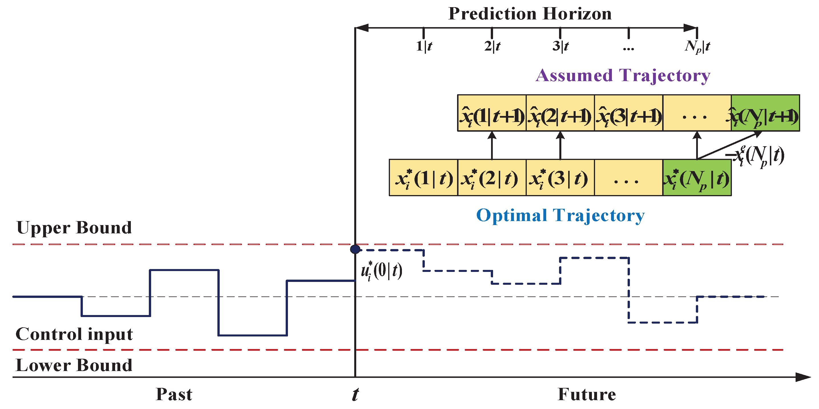
3.4. Algorithm of Distributed Receding Horizon Optimization

In order to address the cooperative driving issue of mixed-automated vehicles at intersections, we present a distributed optimization algorithm under a receding horizon framework. The details are provided in Algorithm 2, which aims to find the optimal solutions for each AV in the CZ by solving (15). Figure 3 shows the basic procedure of the distributed receding horizon optimization scheme. The optimization problem is solved at each time step, and only the first element of the obtained control sequence is applied.

In Algorithm 2, initialization is conducted in step 1, which determines the start time of the algorithm, i.e., when ego AV i enters the CZ, and calculates initial $N_p$-step prediction states $\widehat{x_i}(k+1|0)={[{\widehat{p}}_{ih}(k+1|0),{\widehat{v}}_{ih}(k+1|0)]}^T$, $k=0,\dots ,N_p-1$, using (10). The communication topology of vehicles in the CZ at the current time step is identified in step 3. Based on the communication topology, ego AV i receives the information of $N_p$-step prediction states $\widehat{x_j}(k+1|t)$, $k=0,\dots ,N_p-1$, of neighboring vehicle $j,j\in {\mathcal{N}}_i\left(t\right)$ in step 4. Then, in step 5, ego AV i utilizes its current state and the predicted future $N_p$-step trajectories of neighboring vehicle $j,j\in {\mathcal{N}}_i\left(t\right)$ to solve the optimization problem (15). The first element of the obtained optimal control sequence is applied to AV i in step 6, i.e.,  $u_i\left(t\right)=u_i^{*}\left(0\right|t)$. The prediction of the trajectory of the neighboring vehicles is the key to solving the optimization problem (15) for the ego vehicle. Note that in the framework of distributed cooperation, the communication, computation, and control of all vehicles are assumed to be synchronous. Therefore, each AV i cannot receive the accurate $N_p$-step predicted trajectories of its neighboring vehicle j at the current step. To address this issue, we perform an operation to adopt the $N_p$-step assumed trajectories of neighboring vehicle j in the last shifted time window. Here, we take vehicle $i,i\in {\mathsf{\Omega }}_A\left(t\right)$ as an example and illustrate the calculation process of the assumed trajectory, as depicted in Figure 3. Define $u_i^{*}\left(k\right|t),k=0,\dots ,N_p-1$ as the optimal control sequence, and $x_i^{*}(k+1|t)={[p_{ih}^{*}(k+1|t),v_{ih}^{*}(k+1|t)]}^T,k=0,\dots ,N_p-1$ are the optimal states calculated by (10) in step 7. The assumed trajectory of vehicle i is computed in step 8 by removing the first state value of $x_i^{*}(k+1|t)$, $k=0,\dots ,N_p-1$, and adding the ending value $x_i^{*}\left(N_p\right|t)-x_i^e\left(N_p\right|t)$, where $x_i^e\left(N_p\right|t)={[v_{ih}^{*}\left(N_p\right|t)\delta ,0]}^T.$ The obtained assumed trajectory of vehicle i is transmitted to vehicle j, $j\in {\mathcal{D}}_i\left(t\right)$, and is regarded as the predicted trajectory of vehicle i in the next time window. In the same way, vehicle i receives the assumed trajectory of its neighboring vehicle j, $j\in {\mathcal{N}}_i\left(t\right)$. Note that if vehicle j is an MV, Equation (11) should be used to calculate the assumed trajectory of vehicle j. Similar approaches can be found in [33,35]. In the next shifted time window, the problem is reformulated and solved again until ego AV i departs from the CZ.

Algorithm 2 Algorithm of Distributed Receding Horizon Optimization

Input:  The communication topology of vehicles in the CZ; the state of ego AV $i,i\in {\mathsf{\Omega }}_A\left(t\right)$; $N_p$-step prediction states of its neighboring vehicle $j,j\in N_i\left(t\right)$ Output:  Optimal trajectory of AV i. 1: Initialization: At time $t=0$ (the moment AV i enters the CZ), load the current state ${\overline{x}}_i\left(0\right|0)$; Assume $u_i\left(k\right|0)=0,k=0,\dots ,N_p-1$, and calculate the $N_p$-step prediction states $\widehat{x_i}(k+1|0)$, $k=0,\dots ,N_p-1$, using (10). 2: Repeat 3: Topology identification: Acquire the communication topology of vehicles at the current step. 4: Information reception: Receive the information of $N_p$-step prediction states $\widehat{x_j}(k+1|t)$, $k=0,\dots ,N_p-1$, of neighbor vehicle $j,j\in {\mathcal{N}}_i\left(t\right)$. 5: Optimization solution: At time $t>0$, according to the current state ${\overline{x}}_i\left(0\right|t)$ and received $\widehat{x_j}(k+1|t)$, $k=0,\dots ,N_p-1$, solve the optimal problem (15) and obtain the optimal control sequence $u_i^{*}\left(k\right|t),k=0,\dots ,N_p-1$. 6: Implementation of optimal results: Apply the first element of the optimal control sequence to AV i, i.e., $u_i\left(t\right)=u_i^{*}\left(0\right|t)$. 7: Iteration of optimal states: Calculate the optimal states $x_i^{*}(k+1|t),k=0,\dots ,N_p-1$, by using (10) and $u_i^{*}\left(k\right|t),k=0,\dots ,N_p-1$. 8: Estimation of assumed states: Calculate the $N_p$-step assumed states $\widehat{x_i}(k+1|t+1)$ at time $t+1$ as $$\widehat{x_i}(k+1|t+1)=\left\{\begin{array}{c}{x}_i^{*}(k+2|t),k=0,\dots ,N_p-2\hfill \\ x_i^{*}(k+1|t)-x_i^e(k+1|t),k=N_p-1\hfill \end{array}\right.,$$ then transmit $\widehat{x_i}(k+1|t+1)$ to vehicle $j,j\in {\mathcal{D}}_i\left(t\right)$. 9: Return Optimal trajectory of AV i; 10: $t\leftarrow t+1$ 11: Until Vehicle i departs from the CZ.

Remark 6.

Note that the $N_p$-step predicted trajectories of vehicles might not be entirely calculated since the vehicles may enter the intersection within the prediction horizon. The following operations are conducted to address this issue. (1) By detecting the predicted states of vehicle i, only the predicted information for the valid time steps before vehicle i passes through the stop line is retained, and the information of the remaining steps is set to null. (2) The formulated optimization problem for vehicle i is solved just to obtain the optimization control inputs in the valid time steps. (3) The assumed trajectory of vehicle i is calculated and then transmitted to its neighboring vehicle $j,j\in {\mathcal{N}}_i\left(t\right)$. (4) To maintain the integrity of the received assumed trajectory of vehicle i, the received null values are replaced by the desired assumed state values of the neighboring vehicles of vehicle j. (5) The optimization problem of vehicle j can be solved. The above operations guarantee that if a vehicle enters the intersection at a certain prediction step, the prediction information of the vehicle after this step will not affect the solution of optimization problem (15) for the ego vehicle and its neighboring vehicles.

4. Simulation Results

In this section, simulations are conducted to evaluate the performance of the presented scheme for the cooperative driving of mixed-automated vehicles at an intersection. The proposed algorithm is coded in Python (Version 3.8.13) and run on a computer with Intel Core i5-9500 3 GHz CPU and 8 GB of DDR4-2666 RAM. The SUMO (Version 1.13.0) microscopic traffic simulator is used to construct the road network, generate traffic flows, and acquire performance measurements [36]. Vehicle information is transmitted between SUMO and our control model in Python through SUMO’s TraCI interface.

4.1. Simulation Framework

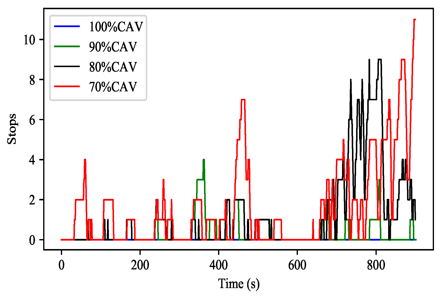
We develop a simulation framework at a single intersection to test the effectiveness of the proposed algorithm in this paper. The test intersection has a typical symmetrical four-leg configuration. The length of each approach and departure section is approximately 193.6 m. Each approach includes two incoming lanes with the specific allowable movements, where the left lane only serves left-turn traffic, and the right lane serves through traffic. The north- and southbound approaches are main roads, and the east- and westbound approaches are minor roads. This distinction allows for the consideration of different traffic priorities and behaviors at the intersection. The radius of the cooperative zone is set as 100 m. The simulation duration is 1 h. Other simulation parameter settings can be seen in

Table 1. Parameter settings.

Parameter	Notation	Value
Common
Radius of CZ (m)	R	100
Lane length (m)	L	193.6
Lane width (m)	W	3.2
Road speed limit (m/s)	$V_{lim}$	20
Vehicle length (m)	l	5
Minimum gap (m)	$d_m$	5
AVs
Desired spacing (m)	$d_{ij}$	10
Maximum speed (m/s)	${\mathcal{V}}_{max}$	18
Minimum speed (m/s)	${\mathcal{V}}_{min}$	5
Maximum acceleration (m/s${}^2$)	${\mathcal{A}}_{max}$	3
Maximum deceleration (m/s${}^2$)	${\mathcal{A}}_{min}$	3
Prediction horizon (s)	$N_p$	5
Time interval (s)	$\delta$	1
Weight	${\omega }_1$	2
Weight	${\omega }_2$	1
Weight	${\omega }_3$	1
Weight	${\omega }_4$	1
MVs
Maximum speed (m/s)	$V_{max}$	18
Maximum acceleration (m/s${}^2$)	$a_{max}$	3
Maximum deceleration (m/s${}^2$)	$b_{max}$	4
Reaction time of drivers (s)	$\tau$	0.5
Constant	$ϵ$	0.4

.

To investigate the sensitivity of the proposed algorithm, we consider three cases based on different traffic volumes.

Table 2. Demand for different cases.

	North- and Southbound		East- and Westbound
Case	Through Demand (veh/h/lane)	Left-Turn Demand (veh/h/lane)	Through Demand (veh/h/lane)	Left-Turn Demand (veh/h/lane)
1	250	125	150	75
2	300	150	200	100
3	350	175	250	125

summarizes the three cases tested in this study. Since our study focuses on environments with high penetration rates of AVs, for each case, four different penetration rates of AVs (i.e., 70%, 80%, 90%, 100%) are considered to evaluate the validity of the proposed algorithm. In addition, the simulation results in a 15 min period are compared to those under the no-control (NC) operation and fixed-time signal control (FSC) strategy.

4.2. Results

The proposed algorithm is tested under the different demand cases and penetration rates of AVs (PRAs) to investigate the performance of the scheme in this study.

Table 3. Summary of mean travel time (s) for the three cases under different penetration rates of AVs.

Case	Penetration Rate of AVs
	100%	90%	80%	70%
1	30.4	30.8	31.1	31.7
2	30.6	31.5	32.1	32.7
3	30.8	32.3	34.6	39.7

shows the comparison of the mean travel time for the different demand and PRAs. The results show that the mean travel time increases slightly when the PRA decreases in cases 1 and 2. In contrast, the mean travel time for case 3 rises substantially with the reduction in PRA. On the other hand, by comparing the results vertically, it slightly differs in the mean travel time for the different cases under 80% to 100% PRA. Conversely, the mean travel time increases significantly for case 3 under 70% PRA. The results indicate that when the PRA is as low as 70% and the total traffic demand reaches 1800 vehicles per hour, there is a significant adverse effect on the traffic efficiency of the intersection. Compared to the results for under 100% PRA, the mean travel time increases by 28.9% under 70% PRA.

Table 4. Summary of mean fuel consumptions (mL) for the three cases under different penetration rates of AVs.

Case	Penetration Rate of AVs
	100%	90%	80%	70%
1	31.8	31.6	31.4	31.5
2	33.4	33.3	33.5	33.7
3	34.7	35.3	36.4	38.8

shows the results for fuel consumption under the different traffic demand and PRAs, respectively. Similarly, the differences in fuel consumption under different PRAs are less distinct for cases 1 and 2. There are even slight drops in fuel consumption when the PRA decreases, since the additional control cost for the desired performance indexes is reduced. The fuel consumption rises significantly with the decline in PRA in case 3. The results indicate that the proposed scheme has less apparent impact on fuel consumption with different PRAs under low demand, while the differences are distinct under high demand.

Figure 4 shows the mean speed relative rates for case 3 in 15 min under different PRAs. The mean speed relative rate is defined as the ratio of the actual average speed to the desired speed. Figure 4 indicates that the mean speed under higher PRAs is generally closer to the desired speed than that under lower PRAs. In particular, during the 700 to 900 s period, the mean speed relative rate maintains a relatively high value under 90% and 100% PRA, while these drop dramatically under 70% and 80% PRA. This phenomenon occurs since more uncontrolled MVs are loaded onto the network during this period. Multiple MVs slow down or even stop at the intersection for safe passing, resulting in reducing the mean speed of the road network. Figure 5 shows the number of stops for case 3 in 15 min under different PRAs. No stops and a few stops occur in the scenarios of 100% and 90% PRA, respectively. When the PRA drops to 70% and 80%, during the 700 to 900 s period, more vehicles stop at the intersection for safe passing, which leads to queuing. The above results indicate that the decrease in the PRA leads to a decline in the traffic efficiency of the intersection.

To compare the performance of the proposed scheme with other methods used, we test the no-control (NC) operation and fixed-time signal control (FSC) strategy as benchmark baselines at the same intersection. The NC operation means allowing all vehicles to pass through the signal-free intersection by following the driving behaviors of MVs. The cycle time of the FSC system is set as 82 s. The green times of north- and southbound, and east- and westbound are chosen as 20 s and 15 s, respectively. The clearance time is 3 s. Figure 6 shows the trajectories of vehicles for case 3 in 5 min under the different strategies. It is observed that the vehicles with the proposed scheme in this paper adjust their trajectories after entering the CZ. Especially in the scenario of 100% PRA, the vehicles pass through the intersection smoothly. When the PRA is 70%, a few vehicles stop at the intersection. In contrast, the vehicles under NC or FSC frequently stop at the intersection, and lots of queues are formed. Figure 7 shows the speeds of vehicles for case 3 in 5 min under the different strategies. Corresponding to the results in Figure 6, the vehicles using the proposed scheme always pass the intersection without halting (speed greater than zero) under 100% PRA, and a small number of vehicles slow down to zero at the intersection under 70% PRA. When NC or FSC is adopted, more vehicles slow to a stop at the intersection. The above phenomena indicate that the proposed scheme in this paper notably outperforms NC and FSC in smoothing traffic flow and improving mobility. Figure 8 shows the acceleration curves of vehicles with respect to distance under the proposed scheme for case 3 in 5 min. We can easily observe that the vehicles adjust their acceleration significantly after entering the CZ. Notice that the maximum acceleration and deceleration of MVs are 3 m/s${}^2$ and 4 m/s${}^2$ in the scenario of 70% PRA, respectively, while the maximum acceleration and deceleration of AVs are both 3 m/s${}^2$.

Table 5. Summary of performance for case 3 under the proposed scheme, no-control operation, and the fixed-signal control strategy.

Performance	Proposed Scheme		NC	FSC
	100% AV	70% AV
Travel time (s)	30.8	39.7	56.5	60.6
Fuel consumption (mL)	34.7	38.8	53.6	49.5

shows the results of the performance, i.e., travel time and fuel consumption, of the proposed scheme, NC operation, and the FSC strategy. The results show that the proposed scheme outperforms NC and FSC by decreasing the mean travel time by 45.5% and 49.2% under 100% PRA, and by 29.7% and 34.5% under 70% PRA, respectively. In addition, compared to NC and FSC, the proposed scheme reduces the mean fuel consumption by 35.3% and 29.9% under 100% PRA, and by 27.6% and 21.6% under 70% PRA, respectively. Overall, the proposed scheme of this paper significantly improves traffic efficiency and fuel economy compared to NC and FSC.

Figure 9 shows the mean speed of the road network with the different strategies for case 3 in 15 min, which reflects the traffic mobility to some extent. The vehicles with the proposed scheme in this study can always maintain a high mean speed in the scenario of 100% PRA. When the PRA is 70%, the mean speed declines, since more MVs are loaded onto the network and slow down at the intersection. In contrast, the mean speed of vehicles under NC or FSC is kept at a smaller value, reflecting the inefficiency of the traffic. Figure 10 shows the number of stops for case 3 in 15 min under the different strategies. It is easy to observe that almost no stops occur in the scenario of 100% PRA with the proposed scheme, and a small number of stops exist under 70% PRA. When NC or FSC is adopted, many vehicles stop near the intersection, leading to queuing. Figure 9 and Figure 10 indicate that the proposed scheme in this paper can significantly improve mobility and smooth traffic flows compared to the NC operation and FSC strategy.

Since few of the current state-of-practice strategies consider mixed-automated traffic at signal-free intersections, we have compared the results of the proposed scheme with a recently developed strategy that jointly optimized the signal timing plans with the trajectory of vehicles in Ramin et al. [24]. The paper developed a centralized mixed-integer non-linear program to coordinate the trajectories of AVs and signal timing plans under mixed-automated traffic. We adopt the same traffic parameters as [24] for comparative simulations under the two-levels of traffic demands, i.e., demand 1 and demand 2. Demand 1 denotes low traffic demand, with 300 veh/h/lane through demand and 24 veh/h/lane left-turn demand, and demand 2 represents high traffic demand, with 600 veh/h/lane through demand and 48 veh/h/lane left-turn demand.

Table 6. Comparison of total delays (s) between the scheme of this paper and Ramin et al. [24] for the two demands under different penetration rates of AVs.

PRA	Demand 1		Demand 2
	This Study	Ramin et al. [24]	This Study	Ramin et al. [24]
100%	69.1	78.2	157.8	173.2
70%	164.2	191.6	1062.3	1057.0
50%	211.7	204.3	1552.1	1363.2
30%	265.6	228.3	2521.6	2000.1
0%	318.4	270.9	3256.2	2468.8

shows the total delay between the scheme proposed in this paper and in [24] for the two demands under different PRAs in 5 min. The results indicate that the total delay increases with PRA reduction in both schemes. In addition, our proposed scheme performs better than [24] under high PRAs and low traffic demand. However, when the PRA drops below 70%, especially under high demand, the total delay in our scheme is higher than in [24]. This suggests that the role of signal timing optimization in [24] is more significant under high demand and a low PRA.

Table 7. Comparison of complexity parameters between the scheme of this paper and Ramin et al. [24] for demand 2 under different penetration rates of AVs.

PRA	# Var.		# Con.		# Com.
	This Study	Ramin et al. [24]	This Study	Ramin et al. [24]	This Study	Ramin et al. [24]
100%	25.5	150.9	20.4	92.8	26.5	38.8
70%	20.3	130.3	16.2	88.5	21.6	33.0
50%	15.5	72.7	12.4	84.4	18.4	29.1
30%	10.4	51.3	5.2	82.0	15.1	25.3
0%	0	15.9	0	75.0	10.2	19.4

# Var.: Mean number of variables per second. # Con.: Mean number of constraints per second. # Com.: Mean number of communications per second.

shows the computation performance between the proposed scheme in this paper and [24] for demand 2 under different PRAs. The parameters # Var. and # Con. denote the mean number of variables and constraints processed per second, and # Com. represents the mean number of communications required per second. The results show that the mean number of variables, constraints, and communications mostly decrease as PRA decreases in both schemes. In addition, the proposed scheme in this paper has fewer computation parameters to process per second than [24], which means that our scheme has an advantage in computational complexity.

4.3. Discussion and Limitations

The existing literature on regulating mixed-automated traffic flow at intersections has focused on introducing traffic lights for right-of-way allocation, e.g., [23,24]. Our study attempts to optimize the behavior of AVs by predicting the trajectory of AVs and MVs, which leads all vehicles to pass through the signal-free intersection without collision and results in a satisfactory traffic performance. Compared to the strategies of jointly optimizing vehicle trajectories and signal timing, our scheme theoretically makes full use of right-of-way without idling caused by traffic lights. However, the increasing number of non-optimized MVs affects the performance of the proposed scheme. In other words, our scheme is sensitive to the PRA and traffic demand. Through the comparison simulation with [24], we find that our scheme performed better under a high PRA and low traffic demand. The results also imply that the application of signal lights and timing optimization for regulating mixed-automated traffic at intersections are more necessary and superior under a low PRA and high traffic demand. In addition, in terms of computational complexity, the proposed scheme in this paper has a certain computational demand since the optimization problem for each AV is solved at each step. Nevertheless, the proposed scheme still has significant advantages in computation compared MILPs jointly optimizing the vehicle trajectory and signal timing.

5. Conclusions

This paper developed a distributed cooperation scheme for coordinating vehicles at signal-free intersections in a mixed traffic environment of AVs and MVs. The traffic conflict graph was constructed to recognize the communication topologies of the vehicles in conflict relationships, assuming that all AVs and MVs were connected and shared information in the CZ. We formulated the coordination issue into a multi-objective optimization problem, which was solved by optimizing the sum of weighted indexes of the conflict elimination, traffic mobility, and fuel economy in a prediction horizon synchronously. The future trajectories of AVs and MVs, as the inputs of the optimization model, were predicted by using the vehicular longitudinal dynamic model and Krauss car-following model, respectively. To obtain the local optimal solutions, we presented a distributed receding horizon algorithm to calculate the optimal control inputs for each AV in the CZ. The simulations evaluated the effectiveness and superiority of the proposed scheme. The results showed that the proposed scheme outperformed the no-control operation by decreasing travel time by 29.7–45.5%, and reducing fuel consumption by 27.6–35.3% under 70–100% PRA. Compared to the fixed-time signal control strategy, the proposed scheme decreased travel time by 34.5–49.2% and reduced fuel consumption by 21.6–29.9% under 70–100% PRA. Additionally, according to the comparison results with the strategy of jointly optimizing the vehicle trajectory and signal timing, the proposed scheme performs better at high penetration rates of AVs and under not very dense traffic demand, and suffers less computational burden.

Though this study considers a typical dual-lane intersection with four approaches, it can be easily extended to on-ramps of expressways or other types of intersections according to the conflict relationships. In addition, advanced driver guidance systems for MVs are expected to be integrated into the intersection coordination framework in future studies. Based on the prompt information of the system, the drivers of MVs can actively manipulate the vehicles to cross the intersection safely and smoothly. In addition, the combination of artificial intelligence methods and other types of optimization methods with the proposed strategy of this paper will be further considered in the future. Furthermore, research on the distributed collaboration of multiple signal-free intersections will be studied under a mixed traffic environment.

References

1. Alanazi, F. A systematic literature review of autonomous and connected vehicles in traffic management. Appl. Sci. 2023, 13, 1789. [Google Scholar] [CrossRef]
2. Sun, K.; Zhao, X.; Gong, S.; Wu, X. A cooperative lane change control strategy for connected and automated vehicles by considering preceding vehicle switching. Appl. Sci. 2023, 13, 2193. [Google Scholar] [CrossRef]
3. Antonio, G.P.; Maria-Dolores, C. Multi-agent deep reinforcement learning to manage connected autonomous vehicles at tomorrow’s intersections. IEEE Trans. Vehi. Technol. 2022, 71, 7033–7043. [Google Scholar] [CrossRef]
4. Feng, Y.; Huang, S.E.; Wong, W.; Chen, Q.A.; Mao, Z.M.; Liu, H.X. On the cybersecurity of traffic signal control system with connected vehicles. IEEE Trans. Intell. Transp. Syst. 2022, 23, 16267–16279. [Google Scholar] [CrossRef]
5. Riostorres, J.; Malikopoulos, A.A. A Survey on the coordination of connected and automated vehicles at intersections and merging at highway on-Ramps. IEEE Trans. Intell. Transp. Syst. 2017, 18, 1066–1077. [Google Scholar] [CrossRef]
6. Dresner, K.; Stone, P. Multiagent traffic management: A reservation-based intersection control mechanism. In Proceedings of the 3rd International Joint Conference on Autonomous Agents and Multiagent Systems: (AAMAS), New York, NY, USA, 19–23 July 2004; pp. 530–537. [Google Scholar]
7. Dresner, K.M.; Stone, P. A Multiagent approach to autonomous intersection management. J. Artif. Intell. Res. 2008, 31, 591–656. [Google Scholar] [CrossRef]
8. Milanes, V.; Perez, J.; Onieva, E.; Gonzalez, C. Controller for urban intersections based on wireless communications and fuzzy logic. IEEE Trans. Intell. Transp. Syst. 2010, 11, 243–248. [Google Scholar] [CrossRef]
9. Onieva, E.; Milanes, V.; Villagra, J.; Perez, J.; Godoy, J. Genetic optimization of a vehicle fuzzy decision system for intersections. Expert Syst. Appl. 2012, 39, 13148–13157. [Google Scholar] [CrossRef]
10. Medina, A.I.M.; van de Wouw, N.; Nijmeijer, H. Cooperative intersection control based on virtual platooning. IEEE Trans. Intell. Transp. Syst. 2017, 19, 1727–1740. [Google Scholar] [CrossRef]
11. Xu, B.; Li, S.E.; Bian, Y.; Li, S.; Ban, X.J.; Wang, J.; Li, K. Distributed conflict-free cooperation for multiple connected vehicles at unsignalized intersections. Transp. Res. C Emerg. Technol. 2018, 93, 322–334. [Google Scholar] [CrossRef]
12. Lee, J.; Park, B. Development and evaluation of a cooperative vehicle intersection control algorithm under the connected vehicles environment. IEEE Trans. Intell. Transp. Syst. 2012, 13, 81–90. [Google Scholar] [CrossRef]
13. Dai, P.; Liu, K.; Zhuge, Q.; Sha, E.H.M.; Lee, V.C.S.; Son, S.H. Quality-of-experience-oriented autonomous intersection control in vehicular networks. IEEE Trans. Intell. Transp. Syst. 2016, 17, 1956–1967. [Google Scholar] [CrossRef]
14. Xu, H.; Zhang, Y.; Li, L.; Li, W. Cooperative driving at unsignalized intersections using tree search. IEEE Trans. Intell. Transp. Syst. 2019, 21, 4563–4571. [Google Scholar] [CrossRef]
15. Meng, Y.; Li, L.; Wang, F.Y.; Li, K.; Li, Z. Analysis of cooperative driving strategies for non-signalized intersections. IEEE Trans. Veh. Technol. 2018, 67, 2900–2911. [Google Scholar] [CrossRef]
16. Gong, J.; Cao, J.; Zhao, Y.; Wei, Y.; Guo, J.; Huang, W. Sampling-based cooperative adaptive cruise control subject to communication delays and actuator lags. Math. Comput. Simul. 2020, 171, 13–25. [Google Scholar] [CrossRef]
17. Lu, J.; Wang, Y.; Shi, X.; Cao, J. Finite-time bipartite consensus for multiagent systems under detail-balanced antagonistic interactions. IEEE Trans. Syst. Man, Cyber. Syst. 2021, 51, 3867–3875. [Google Scholar] [CrossRef]
18. Mirheli, A.; Tajalli, M.; Hajibabai, L.; Hajbabaie, A. A consensus-based distributed trajectory control in a signal-free intersection. Transp. Res. C Emerg. Technol. 2019, 100, 161–176. [Google Scholar] [CrossRef]
19. Zhang, X.; Fang, S.; Shen, Y.; Yuan, X.; Lu, Z. Hierarchical velocity optimization for connected automated vehicles with cellular vehicle-to-everything communication at continuous signalized intersections. IEEE Trans. Intell. Transp. Syst. 2023; early access. [Google Scholar]
20. Kamal, M.A.S.; Imura, J.I.; Hayakawa, T.; Ohata, A.; Aihara, K. A vehicle-intersection coordination scheme for smooth flows of traffic without using traffic lights. IEEE Trans. Intell. Transp. Syst. 2014, 16, 1136–1147. [Google Scholar] [CrossRef]
21. Du, Z.; HomChaudhuri, B.; Pisu, P. Hierarchical distributed coordination strategy of connected and automated vehicles at multiple intersections. J. Intell. Transp. Syst. 2018, 22, 144–158. [Google Scholar] [CrossRef]
22. Pourmehrab, M.; Elefteriadou, L.; Ranka, S.; Martin-Gasulla, M. Optimizing signalized intersections performance under conventional and automated vehicles traffic. IEEE Trans. Intell. Transp. Syst. 2019, 21, 2864–2873. [Google Scholar] [CrossRef]
23. Tajalli, M.; Hajbabaie, A. Traffic signal timing and trajectory optimization in a mixed autonomy traffic stream. IEEE Trans. Intell. Transp. Syst. 2021, 23, 6525–6538. [Google Scholar] [CrossRef]
24. Niroumand, R.; Tajalli, M.; Hajibabai, L.; Hajbabaie, A. Joint optimization of vehicle-group trajectory and signal timing: Introducing the white phase for mixed-autonomy traffic stream. Transp. Res. C Emerg. Technol. 2020, 116, 102659. [Google Scholar] [CrossRef]
25. Xu, H.; Cassandras, C.G.; Li, L.; Zhang, Y. Comparison of cooperative driving strategies for CAVs at signal-free intersections. IEEE Trans. Intell. Transp. Syst. 2021, 23, 7614–7627. [Google Scholar] [CrossRef]
26. Belkhouche, F. Collaboration and optimal conflict resolution at an unsignalized intersection. IEEE Trans. Intell. Transp. Syst. 2018, 20, 2301–2312. [Google Scholar] [CrossRef]
27. Bian, Y.; Li, S.E.; Ren, W.; Wang, J.; Li, K.; Liu, H.X. Cooperation of multiple connected vehicles at unsignalized intersections: Distributed observation, optimization, and control. IEEE Trans. Ind. Electron. 2019, 67, 10744–10754. [Google Scholar] [CrossRef]
28. Li, L.; Wang, F. Cooperative driving at blind crossings using intervehicle communication. IEEE Trans. Veh. Technol. 2006, 55, 1712–1724. [Google Scholar] [CrossRef]
29. Krauß, S. Microscopic Modeling of Traffic Flow: Investigation of Collision Free Vehicle Dynamics. Ph.D. Thesis, University of Cologne, Koln, Germany, 1998. [Google Scholar]
30. Gong, S.; Du, L. Cooperative platoon control for a mixed traffic flow including human drive vehicles and connected and autonomous vehicles. Transp. Res. B Methodol. 2018, 116, 25–61. [Google Scholar] [CrossRef]
31. Rudin, W. Principles of Mathematical Analysis; McGraw-Hill: New York, NY, USA, 1976; Volume 3. [Google Scholar]
32. Ishii, H.; Wang, Y.; Feng, S. An overview on multi-agent consensus under adversarial attacks. Annu. Rev. Control 2022, 53, 252–272. [Google Scholar] [CrossRef]
33. Zheng, Y.; Li, S.E.; Li, K.; Borrelli, F.; Hedrick, J.K. Distributed model predictive control for heterogeneous vehicle platoons under unidirectional topologies. IEEE Trans. Control Syst. Technol. 2017, 25, 899–910. [Google Scholar] [CrossRef]
34. Dunbar, W.B.; Caveney, D.S. Distributed receding horizon control of vehicle platoons: Stability and string stability. IEEE Trans. Autom. Control 2011, 57, 620–633. [Google Scholar] [CrossRef]
35. Dunbar, W.B.; Murray, R.M. Distributed receding horizon control for multi-vehicle formation stabilization. Automatica 2006, 42, 549–558. [Google Scholar] [CrossRef]
36. Lopez, P.A.; Behrisch, M.; Bieker-Walz, L.; Erdmann, J.; Flötteröd, Y.P.; Hilbrich, R.; Lücken, L.; Rummel, J.; Wagner, P.; Wießner, E. Microscopic traffic simulation using sumo. In Proceedings of the 21st International Conference on Intelligent Transportation Systems (ITSC), Maui, HI, USA, 4–7 November 2018; pp. 2575–2582. [Google Scholar]
Figure 1. A scenario of connected vehicles passing through a signal-free intersection.
Applsci 13 11576 g001
Figure 2. Traffic conflict graph for the intersection in Figure 1.
Applsci 13 11576 g002
Figure 3. Illustration of the procedure of the distributed receding horizon optimization scheme.
Applsci 13 11576 g003
Figure 4. Comparison of the mean speed relative rates for case 3 in 15 min under different penetration rates of AVs.
Applsci 13 11576 g004
Figure 5. Comparison of the number of stops for case 3 in 15 min under different penetration rates of AVs.
Applsci 13 11576 g005
Figure 6. The trajectories of vehicles for case 3 in 5 min under the different strategies.
Applsci 13 11576 g006
Figure 7. The speeds of vehicles for case 3 in 5 min under the different strategies.
Applsci 13 11576 g007
Figure 8. The acceleration of vehicles for case 3 in 5 min under the proposed strategy.
Applsci 13 11576 g008
Figure 9. Comparison of the mean speed for case 3 in 15 min under the different strategies: (a) proposed scheme under 100% penetration rate of AVs; (b) proposed scheme under 70% penetration rate of AVs.
Applsci 13 11576 g009
Figure 10. Comparison of the number of stops for Case 3 in 15 min under the different strategies: (a) proposed scheme under 100% penetration rate of AVs; (b) proposed scheme under 70% penetration rate of AVs.
Applsci 13 11576 g010