
Estimation of Grain Size and Composition in Steel Using Laser UltraSonics Simulations at Different Temperatures


Abstract
1. Introduction
- How accurate can grain size be determined from LUS simulations on various simulated microstructures and temperatures?
- How accurate can the phase composition be determined from LUS simulations on various multiphase media and temperatures?
2. Materials and Methods
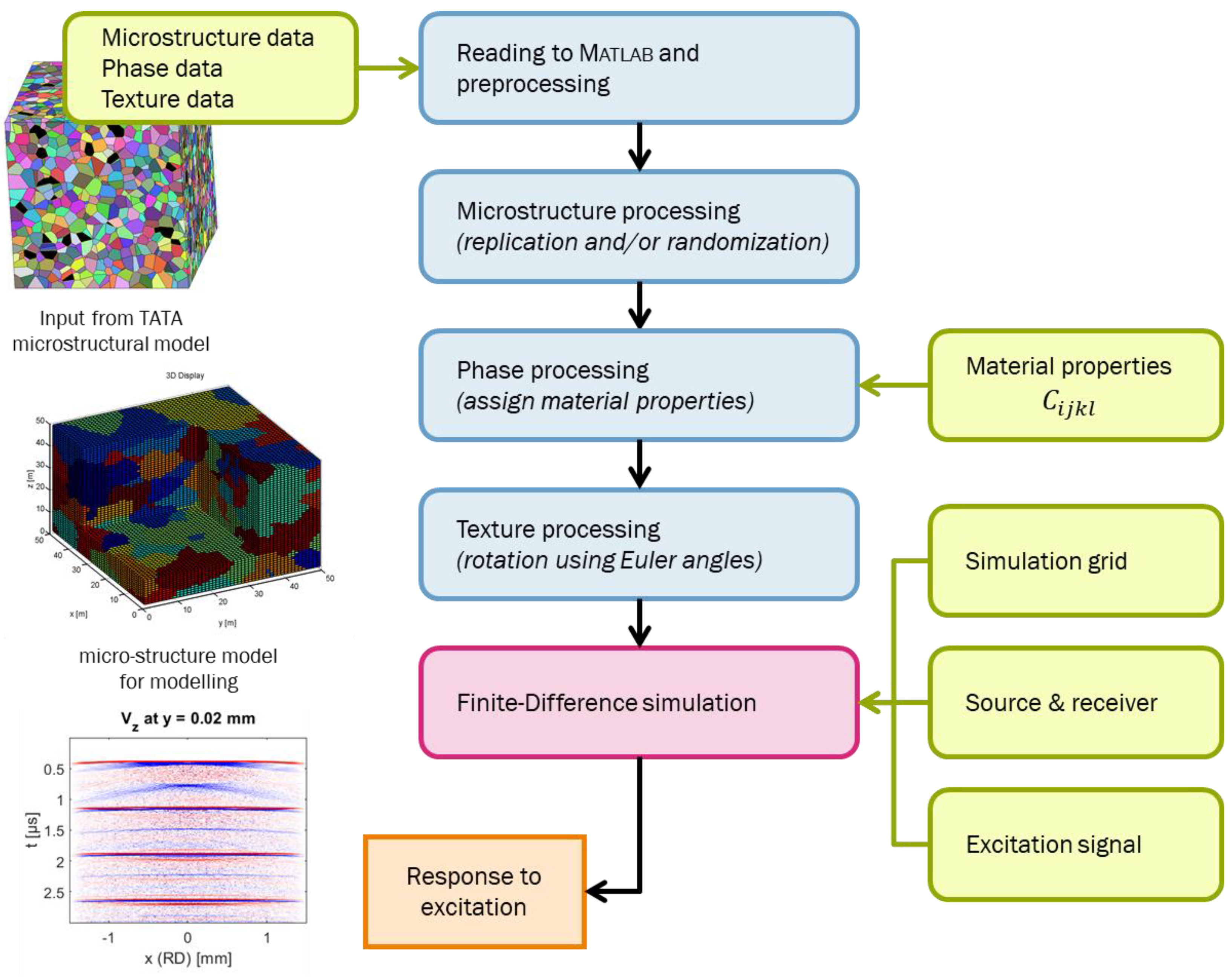
2.1. Simulation Framework
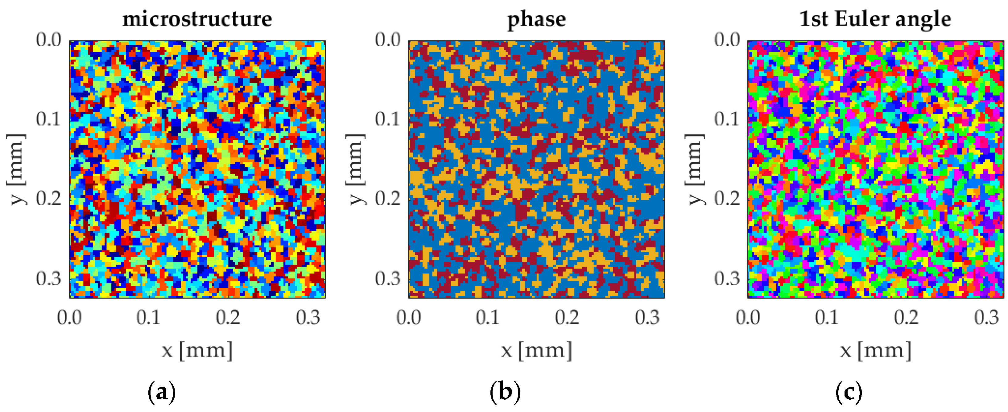
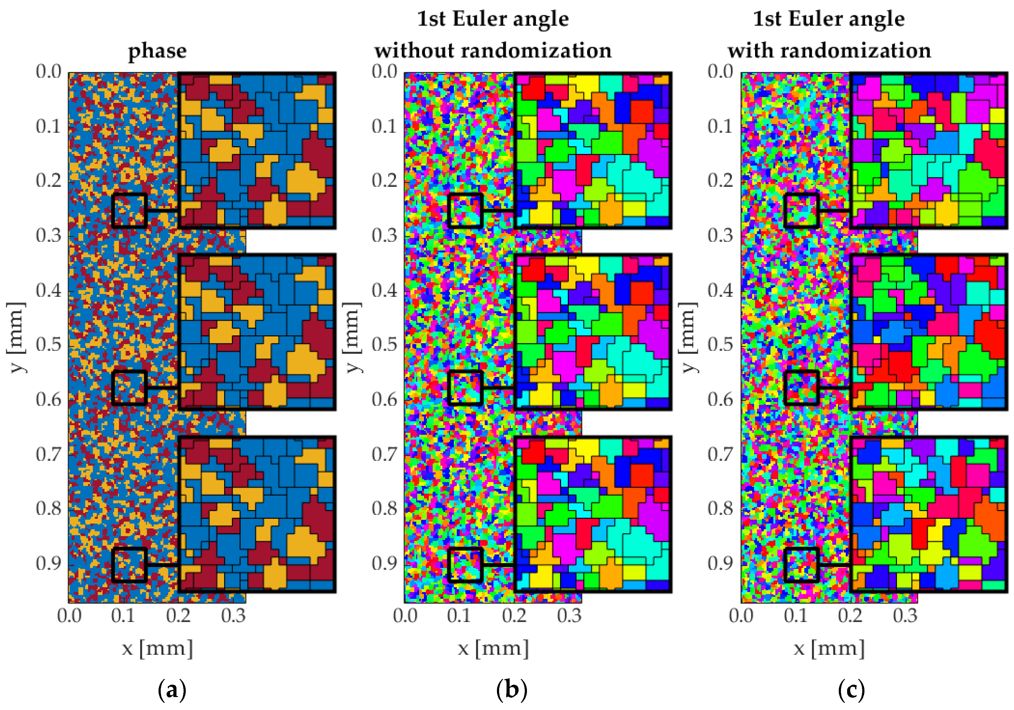
2.2. Fullsize Microstructures
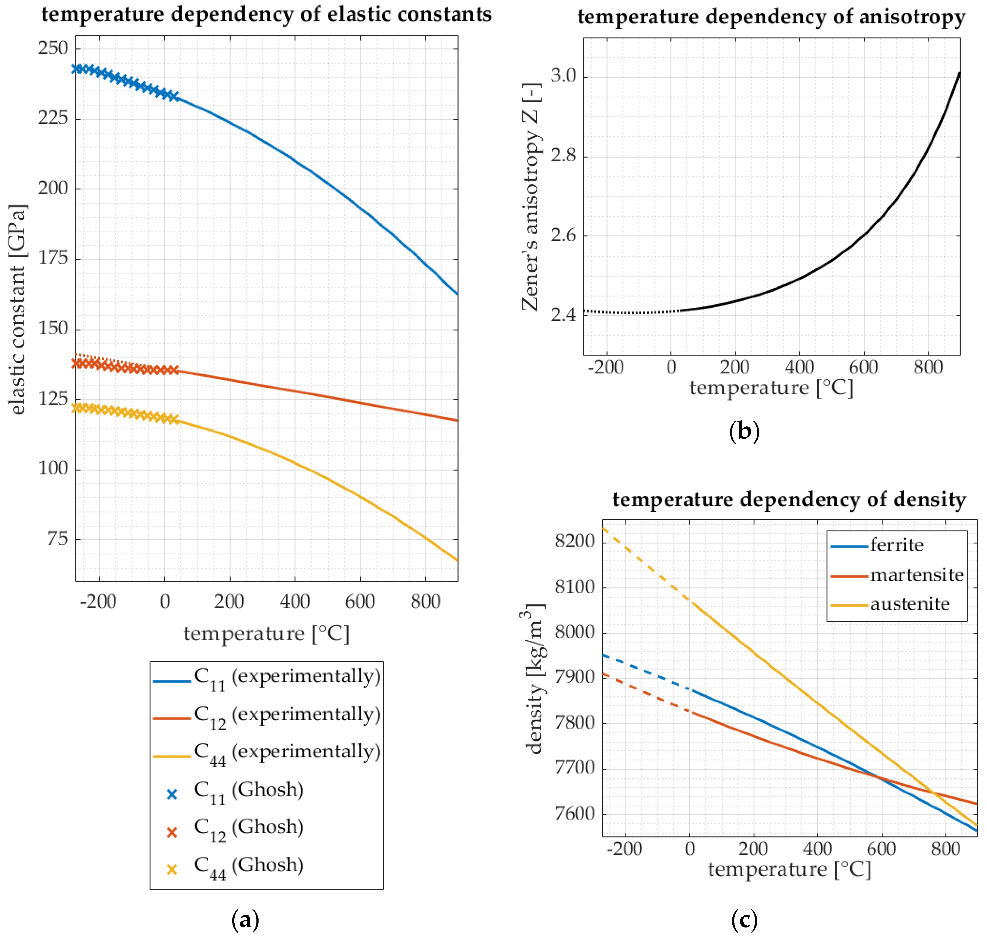
2.3. Temperature-Dependent Material Properties
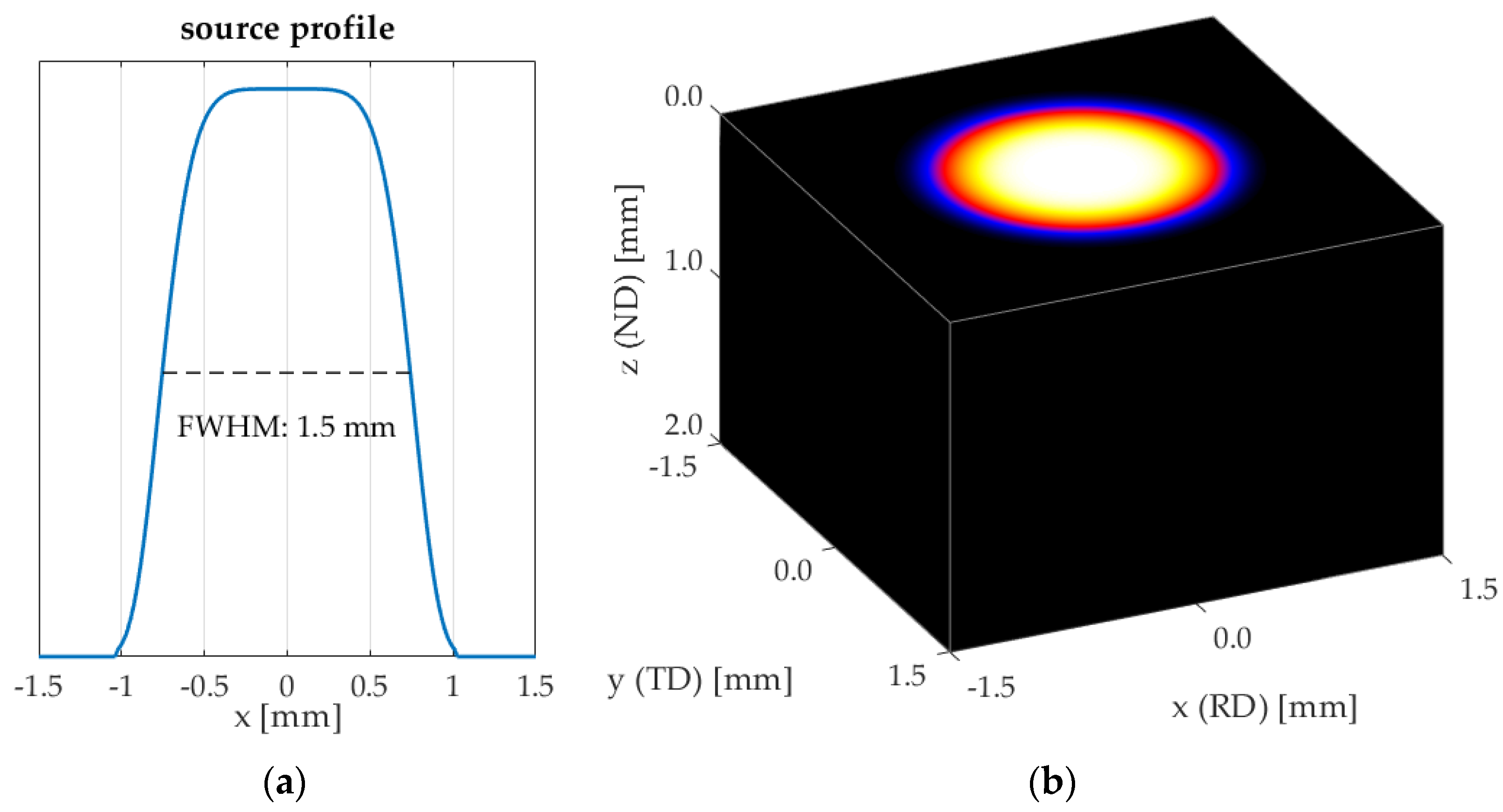
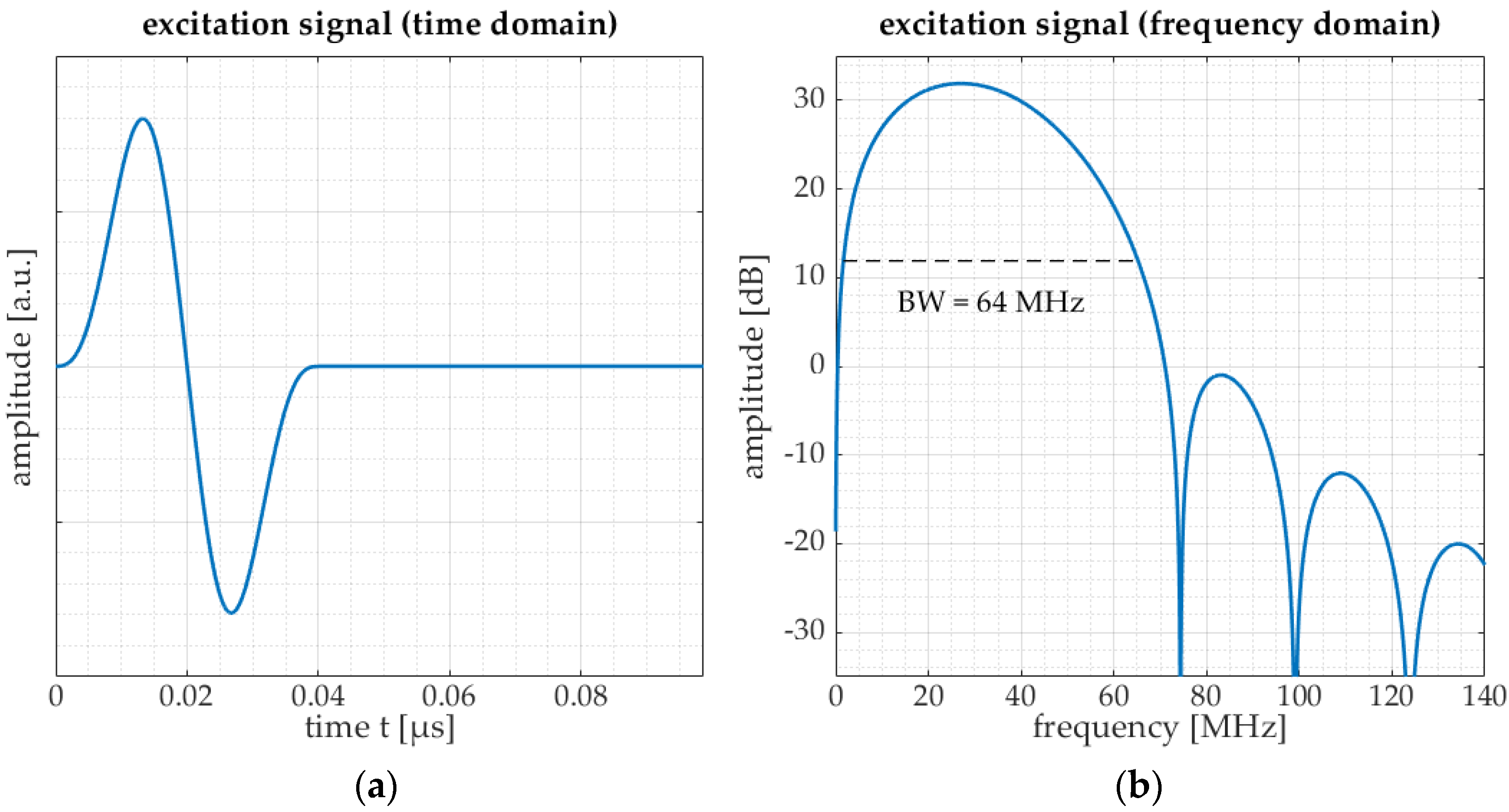
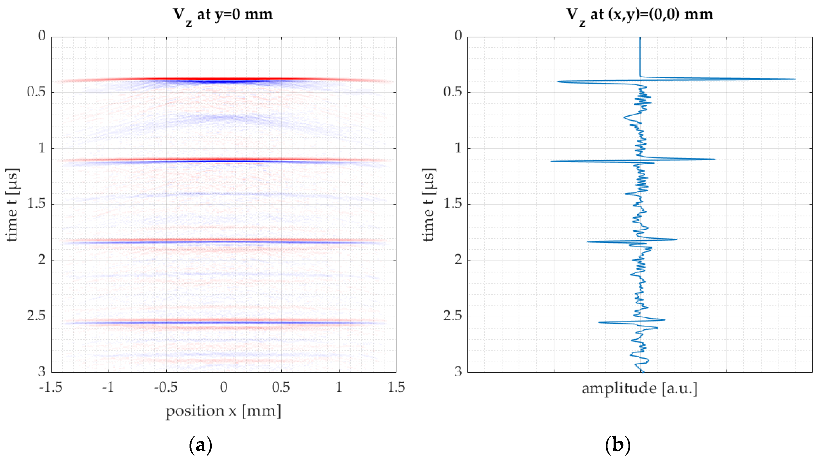
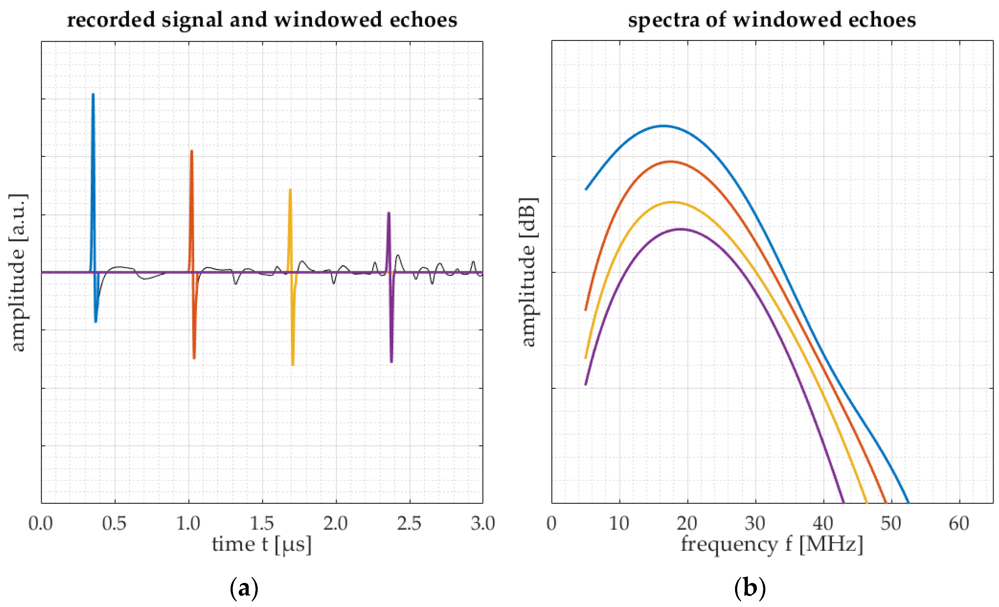
2.4. LUS Modelling, Data Processing and Analysis
- Grain scattering, leading to wave energy dispersion due to mismatches in elasticity in neighboring grains (crystallographic orientation differences due to texture);
- Diffraction of the ultrasonic wave in the medium, affecting both the frequency content as well as the amplitude;
- Absorption of wave energy, which is assumed to be of minor importance to frequency-dependent attenuation.
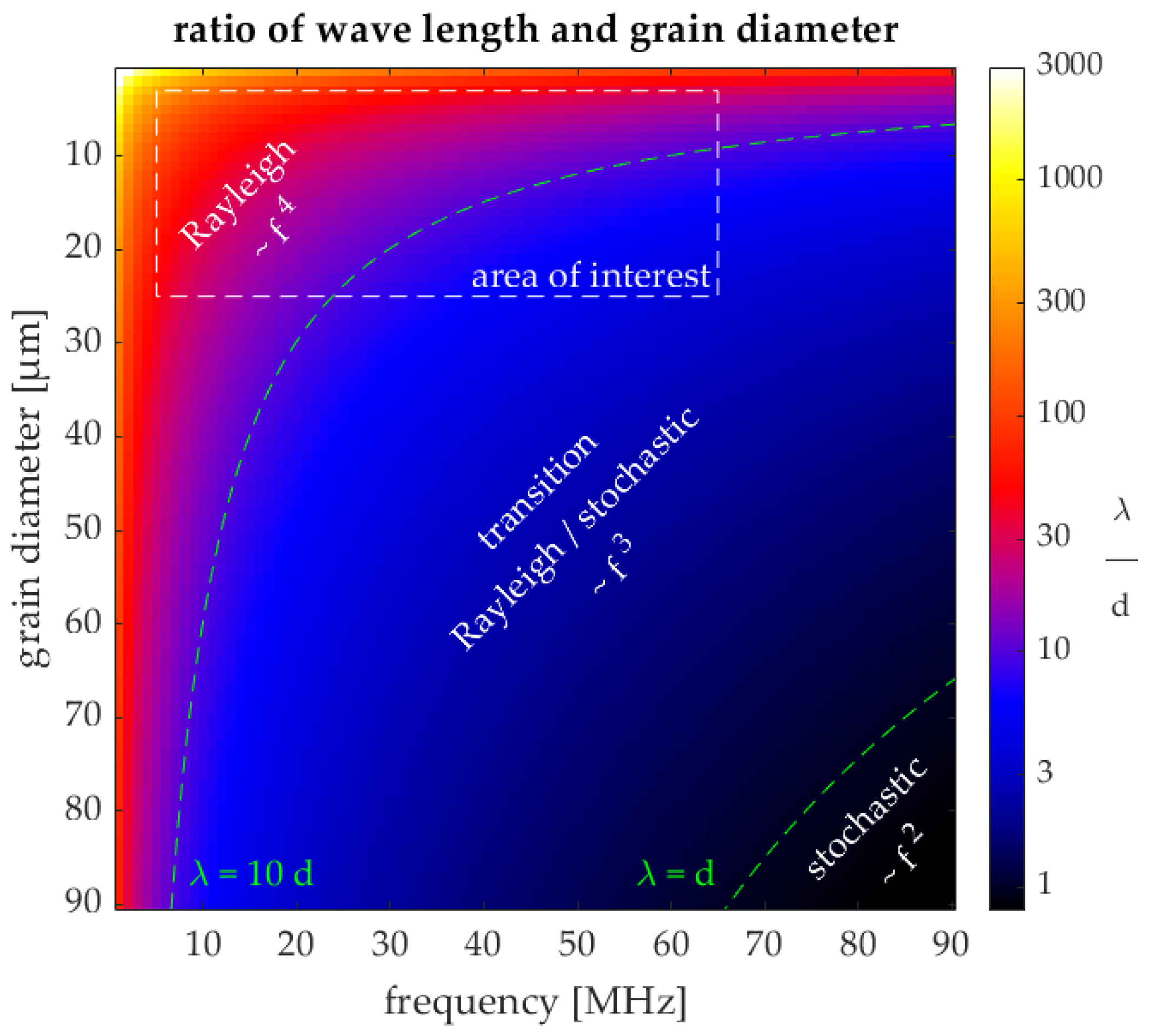
- The Rayleigh regime, where , leading to an attenuation coefficient ;
- The stochastic regime, where , leading to an attenuation coefficient ; and
- The diffusion or geometric regime, where , leading to an attenuation coefficient .
- Compare two echoes of a single measurement, where one echo has travelled a longer distance through the medium than the other and hence has undergone more attenuation due to the medium’s microstructure;
- Compare two echoes from two different measurements (both the same echo number), of which one originates from a well-known medium and the other from the medium to be characterized. Assumed is that the media have the same thickness and hence the waves have travelled the same distance.
3. Results
- The effect of grain size on the 100% austenite samples;
- The effect of grain size on the 100% ferrite samples;
- The effect of phase variation on the austenite/martensite samples;
- The effect of temperature on all samples.
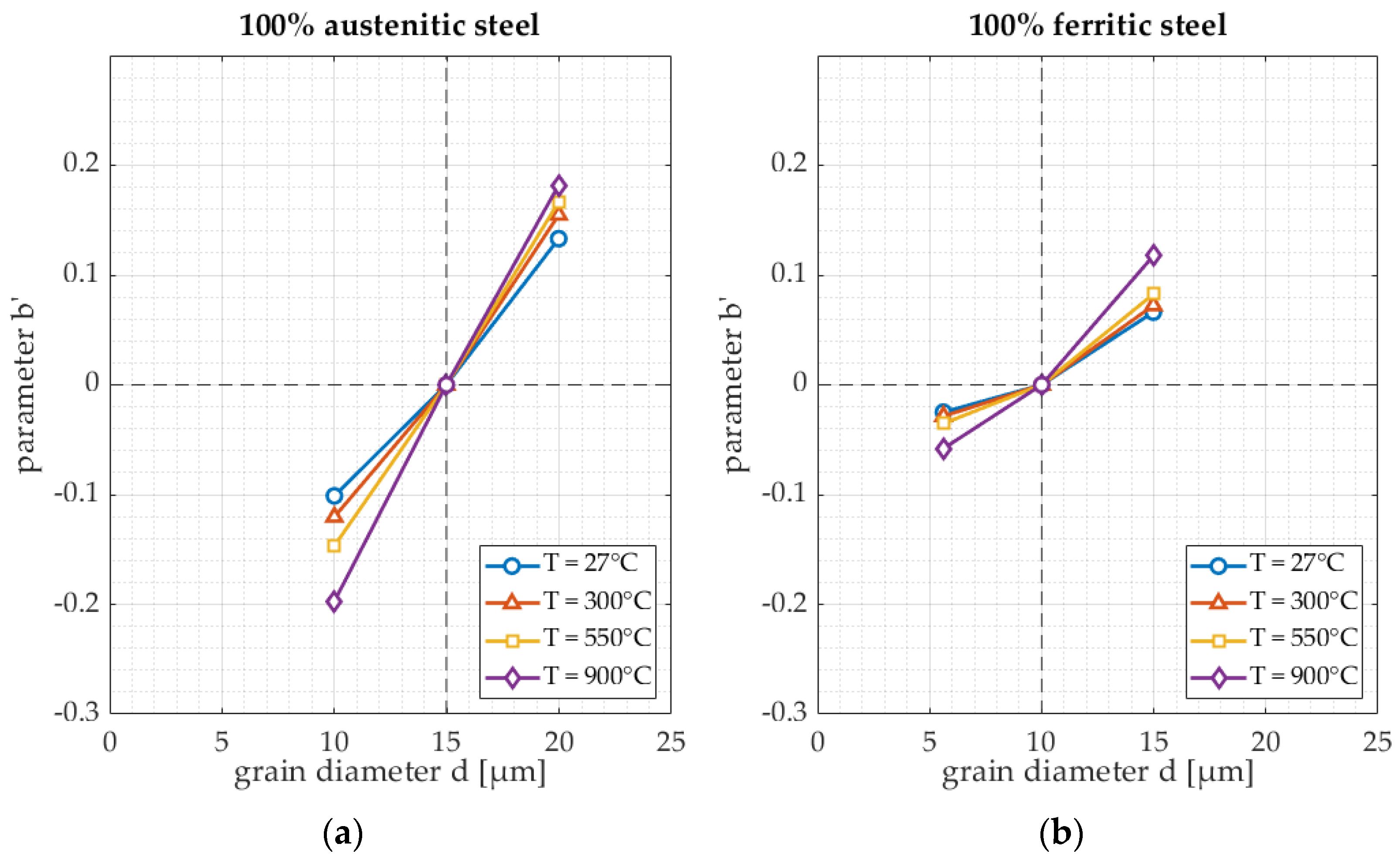
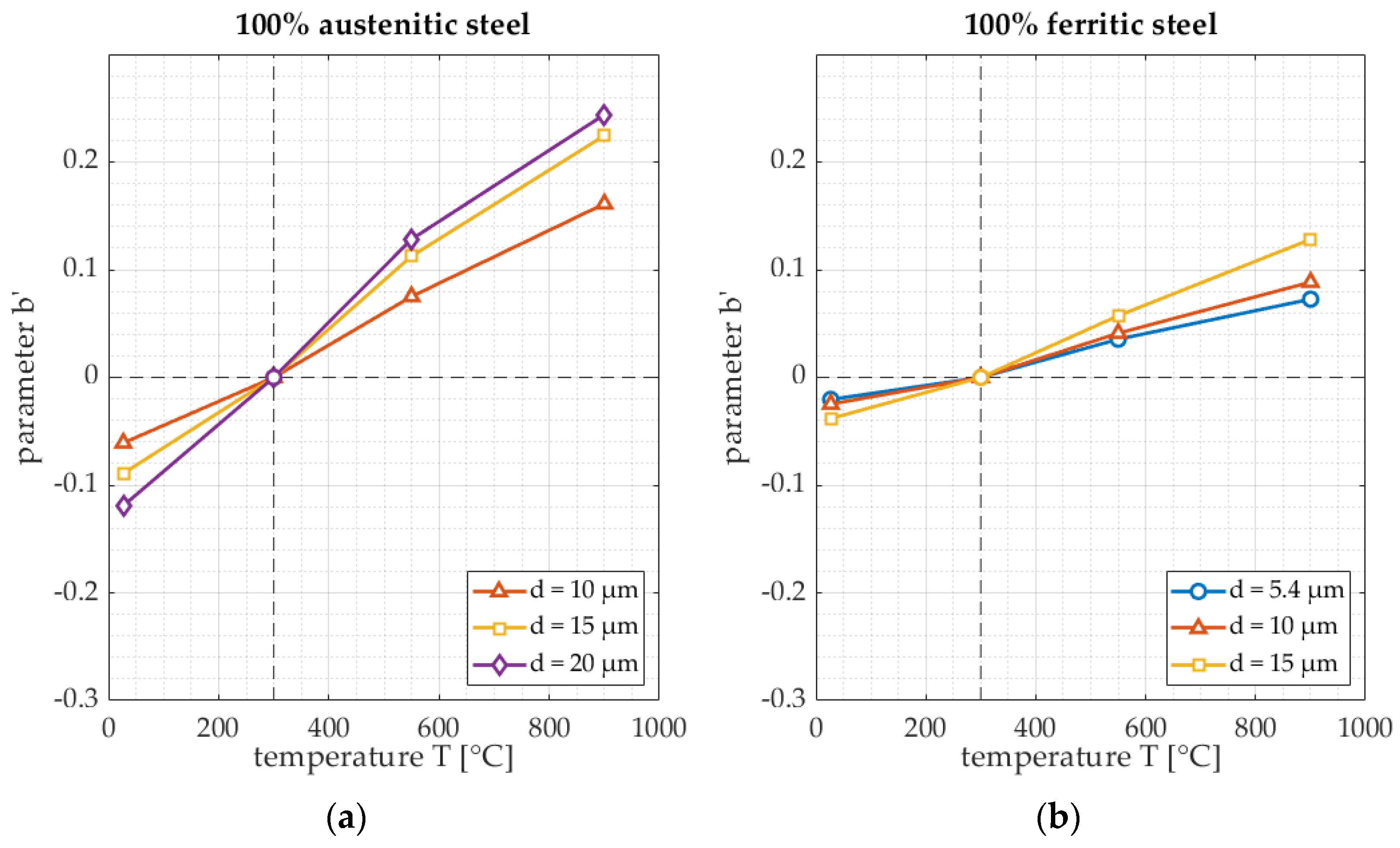
3.1. Microstructure
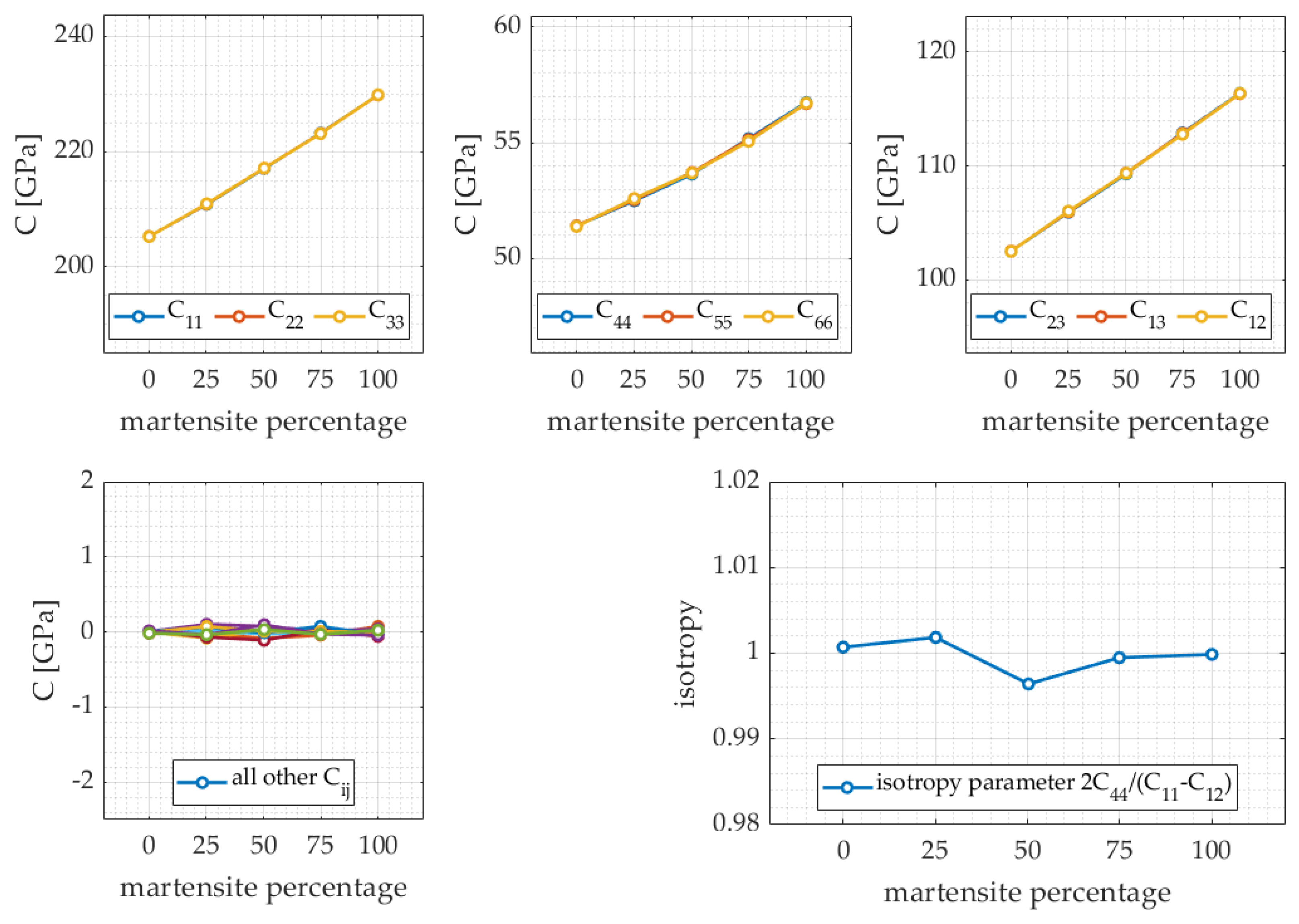
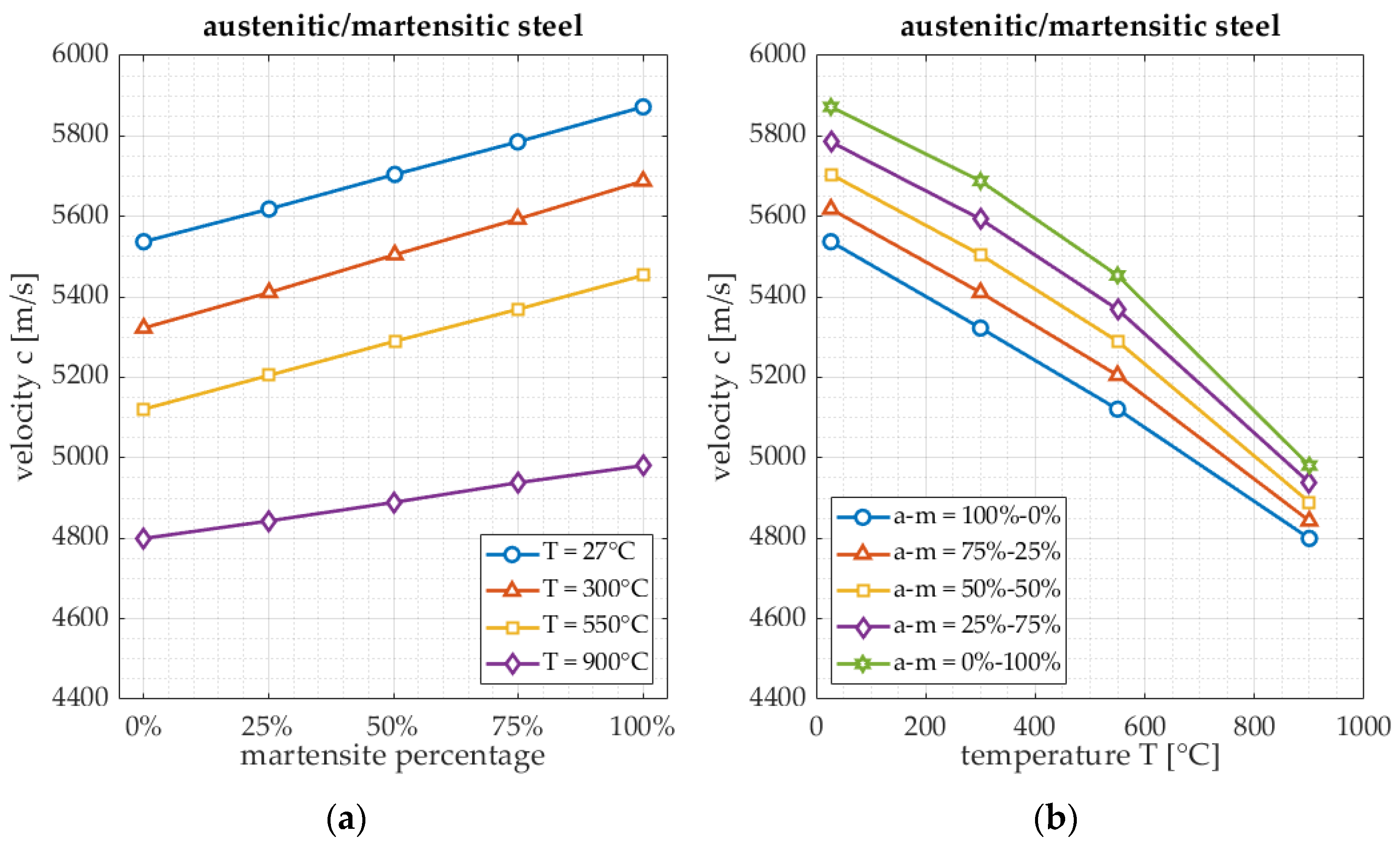
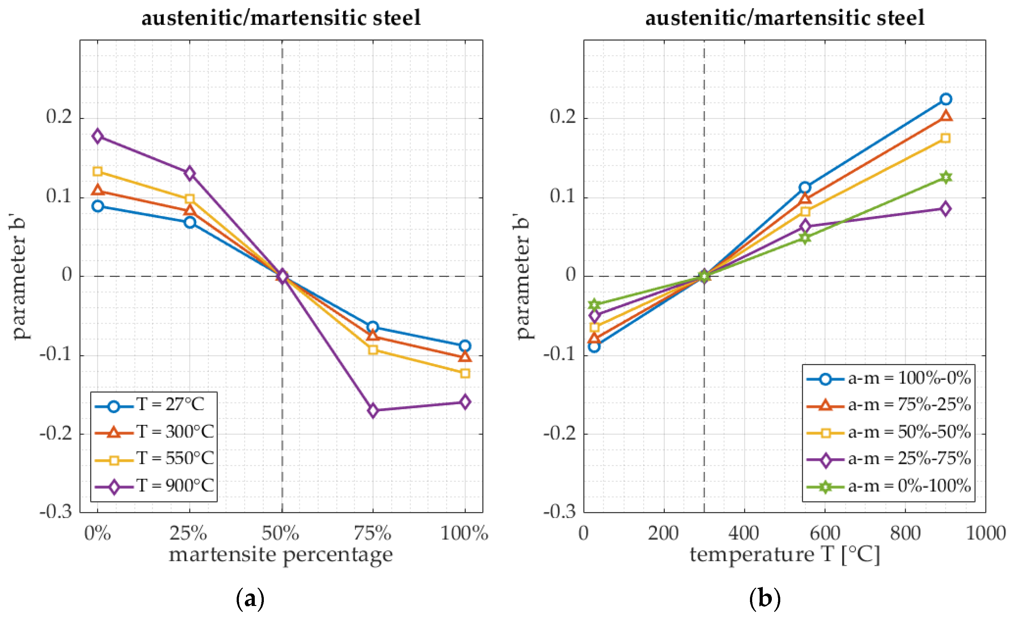
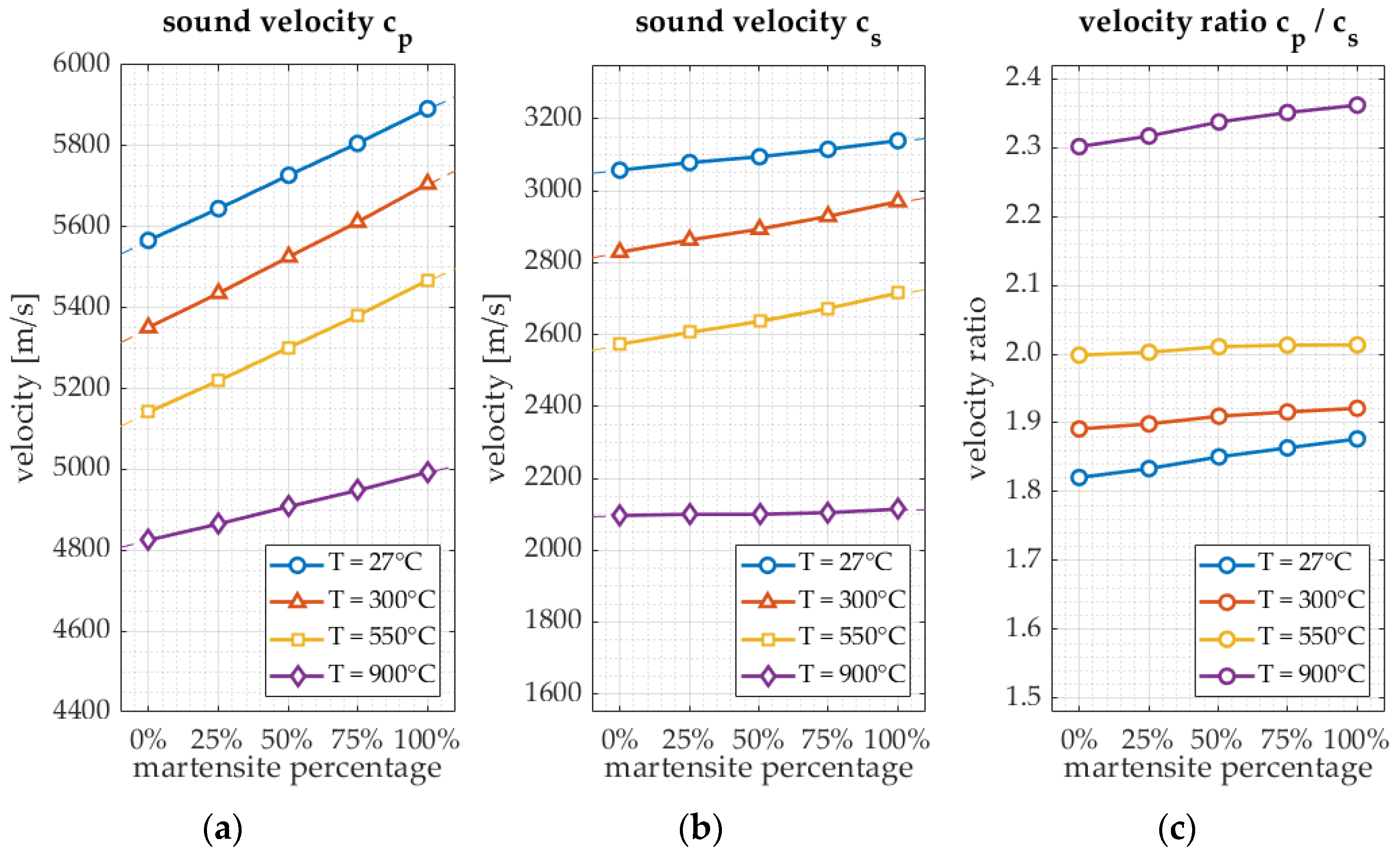
3.2. Multiphase
4. Summary and Discussion
- How accurate can grain size be determined from LUS simulations on various simulated microstructures and temperatures?
- How accurate can the phase composition be determined from LUS simulations on various multiphase media and temperatures?
4.1. Microstructure
4.2. Multiphase
5. Conclusions and Way Ahead
5.1. Conclusions
5.2. Way Ahead
Author Contributions
Funding
Acknowledgments
Conflicts of Interest
References
- Hutchins, D.A.; Dewhurst, R.J.; Palmer, S.B. Laser generation as a standard acoustic source in metals. Appl. Phys. Lett. 1981, 38, 677–679. [Google Scholar] [CrossRef]
- Aindow, A.M.; Dewhurst, R.J.; Palmer, S.B.; Scruby, C.B. Laser-based non-destructive testing techniques for the ultrasonic characterization of subsurface flaws. NDT Int. 1984, 17, 329–335. [Google Scholar] [CrossRef]
- Scruby, C.B.; Smith, R.L.; Moss, B.C. Microstructural monitoring by laser-ultrasonic attenuation and forward scattering. NDT Int. 1986, 19, 307–313. [Google Scholar] [CrossRef]
- Lévesque, D.; Kruger, S.E.; Lamouche, G.; Kolarik, R.; Jeskey, G.; Choquet, M.; Monchalin, J.-P. Thickness and grain size monitoring in seamless tube-making process using laser ultrasonics. NDT E Int. 2006, 39, 622–626. [Google Scholar] [CrossRef]
- Liang, S.; Lévesque, D.; Legrand, N.; Zurob, H.S. Use of in-situ laser-ultrasonics measurements to develop robust models combining deformation, recovery, recrystallization and grain growth. Materialia 2020, 12, 100812. [Google Scholar] [CrossRef]
- Majhi, S.; Mukherjee, A.; George, N.V.; Karaganov, V.; Uy, B. Corrosion monitoring in steel bars using Laser ultrasonic guided waves and advanced signal processing. Mech. Syst. Signal Process. 2021, 149, 107176. [Google Scholar] [CrossRef]
- Ji, B.; Zhang, Q.; Cao, J.; Li, H.; Zhang, B. Non-contact detection of delamination in stainless steel/carbon steel composites with laser ultrasonic. Optik 2021, 226, 165893. [Google Scholar] [CrossRef]
- Sarkar, S.; Moreau, A.; Militzer, M.; Poole, W.J. Evolution of Austenite Recrystallization and Grain Growth Using Laser Ultrasonics. Metall. Mater. Trans. A 2008, 39, 897–907. [Google Scholar] [CrossRef]
- Garcin, T.; Schmitt, J.-H.; Militzer, M. In-situ laser ultrasonic grain size measurement in superalloy INCONEL 718. J. Alloy. Compd. 2016, 670, 329–336. [Google Scholar] [CrossRef]
- Scherleitner, E.; Kerschbaummayr, C.; Haderer, W.; Reitinger, B.; Mitter, T.; Gruensteidl, C. Characterization of Microstructure Variations by Laser-Ultrasound during and after the Heat Treatment of Metals. IOP Conf. Ser. Mater. Sci. Eng. 2021, 1178, 012050. [Google Scholar] [CrossRef]
- Malmström, M.; Jansson, A.; Hutchinson, B. Application of Laser-Ultrasonics for Evaluating Textures and Anisotropy. Appl. Sci. 2022, 12, 10547. [Google Scholar] [CrossRef]
- Scruby, C.B.; Drain, L.E. Laser Ultrasonics, Techniques and Applications; Adam Hilger: Bristol, UK, 1990; ISBN 0-7503-0050-7. [Google Scholar]
- Falkenström, M.; Engman, M.; Lindh-Ulmgren, E.; Hutchinson, B. Laser Ultrasonics for Process Control in the Metal Industry. Nondestruct. Test. Eval. 2011, 26, 237–252. [Google Scholar] [CrossRef]
- Gusev, V.E.; Shen, Z.; Murray, T.W. Special Issue on Laser Ultrasonics. Appl. Sci. 2019, 9, 5561. [Google Scholar] [CrossRef]
- Van den Berg, F. Product Uniformity Control (PUC): Final Report; Publications Office of the European Union: Luxembourg, 2020; ISBN 978-92-76-17320-5. [Google Scholar]
- Monchalin, J.P. Laser-Ultrasonics: Principles And Industrial Applications. E J. Nondestruct. Test. 2020, 1435, 4934. [Google Scholar]
- Everton, S.; Dickens, P.; Tuck, C.; Dutton, B. Using Laser Ultrasound to Detect Subsurface Defects in Metal Laser Powder Bed Fusion Components. J. Miner. Met. Mater. Soc. 2018, 70, 378–383. [Google Scholar] [CrossRef]
- Bakre, C.; Afzalimir, S.H.; Jamieson, C.; Nassar, A.; Reutzel, E.W.; Lissenden, C.J. Laser Generated Broadband Rayleigh Waveform Evolution for Metal Additive Manufacturing Process Monitoring. Appl. Sci. 2022, 12, 12208. [Google Scholar] [CrossRef]
- Dong, F.; Wang, X.; Yang, Q.; Yin, A.; Xu, X. Directional dependence of aluminum grain size measurement by laser-ultrasonic technique. Mater. Charact. 2017, 129, 114–120. [Google Scholar] [CrossRef]
- Malmström, M.; Jansson, A.; Hutchinson, B.; Lönnqvist, J.; Gillgren, L.; Bäcke, L.; Sollander, H.; Bärwald, M.; Hochhard, S.; Lundin, P. Laser-Ultrasound-Based Grain Size Gauge for the Hot Strip Mill. Appl. Sci. 2022, 12, 10048. [Google Scholar] [CrossRef]
- Keyvani, M.; Garcin, T.; Fabrègue, D.; Militzer, M.; Yamanaka, K.; Chiba, A. Continuous Measurements of Recrystallization and Grain Growth in Cobalt Super Alloys. Metall. Mater. Trans. A 2017, 48, 2363–2374. [Google Scholar] [CrossRef]
- Feaugas, X.; Haddou, H. Grain-size effects on tensile behavior of nickel and AISI 316L stainless steel. Metall. Mater. Trans. A 2003, 34, 2329–2340. [Google Scholar] [CrossRef]
- Watzl, G.; Grünsteidl, C.; Arnoldt, A.; Nietsch, J.A.; Österreicher, J.A. In situ laser-ultrasonic monitoring of elastic parameters during natural aging in an Al-Zn-Mg-Cu alloy (AA7075) sheet. Materialia 2022, 26, 101600. [Google Scholar] [CrossRef]
- Wan, T.; Naoe, T.; Wakui, T.; Futakawa, M.; Obayashi, H.; Toshinobu, S. Effects of Grain Size on Ultrasonic Attenuation in Type 316L Stainless Steel. Materials 2017, 10, 753. [Google Scholar] [CrossRef]
- Qin, W.; Li, J.; Liu, Y.; Kang, J.; Zhu, L.; Shu, D.; Peng, P.; She, D.; Meng, D.; Li, Y. Effects of grain size on tensile property and fracture morphology of 316L stainless steel. Mater. Lett. 2019, 254, 116–119. [Google Scholar] [CrossRef]
- Abbasi Aghuy, A.; Zakeri, M.; Moayed, M.H.; Mazinani, M. Effect of grain size on pitting corrosion of 304L austenitic stainless steel. Corros. Sci. 2015, 94, 368–376. [Google Scholar] [CrossRef]
- Su, Y.; Song, R.; Wang, T.; Cai, H.; Wen, J.; Guo, K. Grain size refinement and effect on the tensile properties of a novel low-cost stainless steel. Mater. Lett. 2020, 260, 126919. [Google Scholar] [CrossRef]
- Tasan, C.C.; Hoefnagels, J.; Diehl, M.; Yan, D.; Roters, F.; Raabe, D. Strain localization and damage in dual phase steels investigated by coupled in-situ deformation experiments and crystal plasticity simulations. Int. J. Plast. 2014, 63, 198–210. [Google Scholar] [CrossRef]
- Kadkhodapour, J.; Schmauder, S.; Raabe, D.; Ziaei-Rad, S.; Weber, U.; Bechtold, M. Experimental and numerical study on geometrically necessary dislocations and non-homogeneous mechanical properties of the ferrite phase in dual phase steels. Acta Mater. 2011, 59, 4387–4394. [Google Scholar] [CrossRef]
- Ghassemi-Armaki, H.; Maaß, R.; Bhat, S.P.; Sriram, S.; Greer, J.R.; Kumar, K.S. Deformation response of ferrite and martensite in a dual-phase steel. Acta Mater. 2014, 62, 197–211. [Google Scholar] [CrossRef]
- Pierman, A.-P.; Bouaziz, O.; Pardoen, T.; Jacques, P.J.; Brassart, L. The influence of microstructure and composition on the plastic behaviour of dual-phase steels. Acta Mater. 2014, 73, 298–311. [Google Scholar] [CrossRef]
- Tasan, C.C.; Diehl, M.; Yan, D.; Bechtold, M.; Roters, F.; Schemmann, L.; Zheng, C.; Peranio, N.; Ponge, D.; Koyama, M.; et al. An Overview of Dual-Phase Steels: Advances in Microstructure-Oriented Processing and Micromechanically Guided Design. Annu. Rev. Mater. Res. 2015, 45, 391–431. [Google Scholar] [CrossRef]
- Shivaprasad, S.; Pandala, A.; Krishnamurthy, C.V.; Balasubramaniam, K. Wave localized finite-difference-time-domain modelling of scattering of elastic waves within a polycrystalline material. J. Acoust. Soc. Am. 2018, 144, 3313–3326. [Google Scholar] [CrossRef]
- Shivaprasad, S.; Krishnamurthy, C.V.; Pandala, A.; Saini, A.; Ramachandran, A.; Balasubramaniam, K. Numerical modelling methods for ultrasonic wave propagation through polycrystalline materials. Trans. Indian Inst. Met. 2019, 72, 2923–2932. [Google Scholar] [CrossRef]
- Van Pamel, A.; Brett, C.R.; Huthwaite, P.; Lowe, M.J.S. Finite element modelling of elastic wave scattering within a polycrystalline material in two and three dimensions. J. Acoust. Soc. Am. 2015, 138, 2326–2336. [Google Scholar] [CrossRef]
- Van Pamel, A.; Sha, G.; Rokhlin, S.I.; Lowe, M.J.S. Finite-element modelling of elastic wave propagation and scattering within heterogeneous media. Proc. R. Soc. A 2017, 473, 20160738. [Google Scholar] [CrossRef]
- Hou, R.; Xu, B.; Xia, Z.; Zhang, Y.; Liu, W.; Glorieux, C.; Marsh, J.; Hou, L.; Liu, X.; Xiong, J. Numerical Simulation of Enhanced Photoacoustic Generation and Wavefront Shaping by a Distributed Laser Array. Appl. Sci. 2021, 11, 9497. [Google Scholar] [CrossRef]
- Virieux, J. P-SV wave propagation in heterogeneous media: Velocity-stress finite-difference method. Geophysics 1985, 51, 889–901. [Google Scholar] [CrossRef]
- Saenger, E.H.; Bohlen, T. Finite-difference modeling of viscoelastic and anisotropic wave propagation using the rotated staggered grid. Geophysics 2004, 69, 583–591. [Google Scholar] [CrossRef]
- Celada-Casero, C.; Vercruysse, F.; Linke, B.; Smith, A.; Kok, P.; Sietsma, J.; Santofimia, M.J. Analysis of work hardening mechanisms in Quenching and Partitioning steels combining experiments with a 3D micro-mechanical model. Mater. Sci. Eng. A 2022, 846, 143301. [Google Scholar] [CrossRef]
- Ghosh, G.; Olson, G.B. The isotropic shear modulus of multicomponent Fe-base solid solutions. Acta Mater. 2002, 50, 2655–2675. [Google Scholar] [CrossRef]
- Rayne, J.A.; Chandrasekhar, B.S. Elastic Constants of Iron from 4.2 to 300 °K. Phys. Rev. 1961, 122, 1714–1716. [Google Scholar] [CrossRef]
- Kim, S.A.; Johnson, W.L. Elastic constants and internal friction of martensitic steel, ferritic-pearlitic steel, and α-iron. Mater. Sci. Eng. A 2007, 452–453, 633–639. [Google Scholar] [CrossRef]
- Gunkelmann, N.; Ledbetter, H.; Urbassek, H.M. Experimental and atomistic study of the elastic properties of α′ Fe–C martensite. Acta Mater. 2012, 60, 4901–4907. [Google Scholar] [CrossRef]
- Kamaya, M. A procedure for estimating Young’s modulus of textured polycrystalline materials. Int. J. Solids Struct. 2009, 46, 2642–2649. [Google Scholar] [CrossRef]
- Ledbetter, H.M. Predicted Single-Crystal Elastic Constants of Stainless-Steel 316; Report NBSIR-82-1667; National Bureau of Standards: Washington, DC, USA, 1982. [Google Scholar]
- Gasteau, D.; Chigarev, N.; Ducousso-Ganjehi, L.; Gusev, V.; Jenson, F.; Calmon, P.; Tournat, V. Elastic constants of polycrystalline steel evaluated with laser generated surface acoustic waves. J. Appl. Phys. 2016, 119, 043103. [Google Scholar] [CrossRef]
- Lethbridge, Z.A.D.; Walton, R.I.; Marmier, A.S.H.; Smith, C.W.; Evans, K.E. Elastic anisotropy and extreme Poisson’s ratios in single crystals. Acta Mater. 2010, 58, 6444–6451. [Google Scholar] [CrossRef]
- Hutchinson, B.; Malmström, M.; Lönnqvist, J.; Bate, P.; Ehteshami, H.; Korzhavyi, P.A. Elasticity and Wave Velocity in Fcc Iron (Austenite) at Elevated Temperatures–Experimental Verification of Ab-Initio Calculations. Ultrasonics 2018, 87, 44–47. [Google Scholar] [CrossRef]
- Duijster, A.; Volker, A.; van den Berg, F.; Celada-Casero, C.; Melzer, S. Estimation of the stiffness tensor from Lamb wave velocity profiles measured on steel with different texture. European Conference on Non-Destructive Testing 2023 (ECNDT 2023), 2023; in press. [Google Scholar]
- Cho, Y.-G.; Kim, J.-Y.; Cho, H.-H.; Cha, P.-R.; Suh, D.-W.; Lee, J.K.; Han, H.N. Analysis of Transformation Plasticity in Steel Using a Finite Element Method Coupled with a Phase Field Model. PLoS ONE 2012, 7, e35987. [Google Scholar] [CrossRef] [PubMed]
- Lyassami, M.; Shahriari, D.; Ben Fredj, E.; Morin, J.-B.; Jahazi, M. Numerical Simulation of Water Quenching of Large Size Steel Forgings: Effects of Macrosegregation and Grain Size on Phase Distribution. J. Manuf. Mater. Process. 2018, 2, 34. [Google Scholar] [CrossRef]
- Dubois, M.; Militzer, M.; Moreau, A.; Bussière, J.F. A New Technique for the Quantitative Real-Time Monitoring of Austenite Grain Growth in Steel. Scr. Mater. 2000, 42, 867–874. [Google Scholar] [CrossRef]
- Moreau, A.; Lévesque, D.; Sarkar, S. Laser-Ultrasonics for Metallurgy: Overview and Latest Developments at NRC; NRC Publications Archive; National Research Council: Ottawa, ON, Canada, 2013. [Google Scholar]
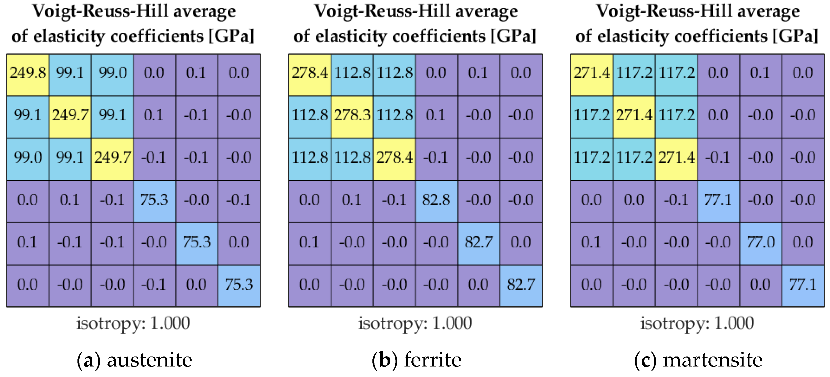
- Kube, C.M.; Turner, J.A. Voigt, Reuss, Hill, and self-consistent techniques for modeling ultrasonic scattering. AIP Conf. Proc. 2015, 1650, 926–934. [Google Scholar]


| Material | ||||||
|---|---|---|---|---|---|---|
| Ferrite [41,42] | Ferrite [43] | Martensite [44] | Austenite [45,46] | Austenite [47] | ||
| Elastic constants [GPa] | 233.1 | 231.5 | 237 | 198 | 192.7 | |
| 233.1 | 231.5 | 237 | 198 | 192.7 | ||
| 233.1 | 231.5 | 256 | 198 | 192.7 | ||
| 135.4 | 135.0 | 144 | 125 | 131.3 | ||
| 135.4 | 135.0 | 144 | 125 | 131.3 | ||
| 135.4 | 135.0 | 144 | 125 | 131.3 | ||
| 117.8 | 116.0 | 115 | 122 | 126.3 | ||
| 117.8 | 116.0 | 115 | 122 | 126.3 | ||
| 117.8 | 116.0 | 115 | 122 | 126.3 | ||
| Zener’s anisotropy | 2.41 | 2.40 | 2.47 | 3.34 | 4.11 | |
| Reference temperature | 300 K (27 °C) | room temperature | 0 K (−273 °C) | not mentioned, assumed 298 K (25 °C) | not mentioned, assumed 298 K (25 °C) | |
| Microstructure Geometry ID | Average Grain Diameter [µm] | Material Properties (Phases and Phase Ratios) | Subset IDs |
|---|---|---|---|
| 1 | 10.0 | 100% Austenite | A, D |
| 2 | 15.0 | 100% Austenite | A, C, D |
| 3 | 20.0 | 100% Austenite | A, D |
| 4 | 5.4 | 100% Ferrite | B, D |
| 5 | 10.0 | 100% Ferrite | B, D |
| 6 | 15.0 | 100% Ferrite | B, D |
| 7 | A: 15.0, M: 10.0 | 75% Austenite, 25% Martensite | C, D |
| 8 | A: 15.0, M: 10.0 | 50% Austenite, 50% Martensite | C, D |
| 9 | A: 15.0, M: 10.0 | 25% Austenite, 75% Martensite | C, D |
| 10 | 10.0 | 100% Martensite | C, D |
| Sample Characteristic | Impact on the Pressure Wave Velocity | Impact on the Frequency Dependent Attenuation |
|---|---|---|
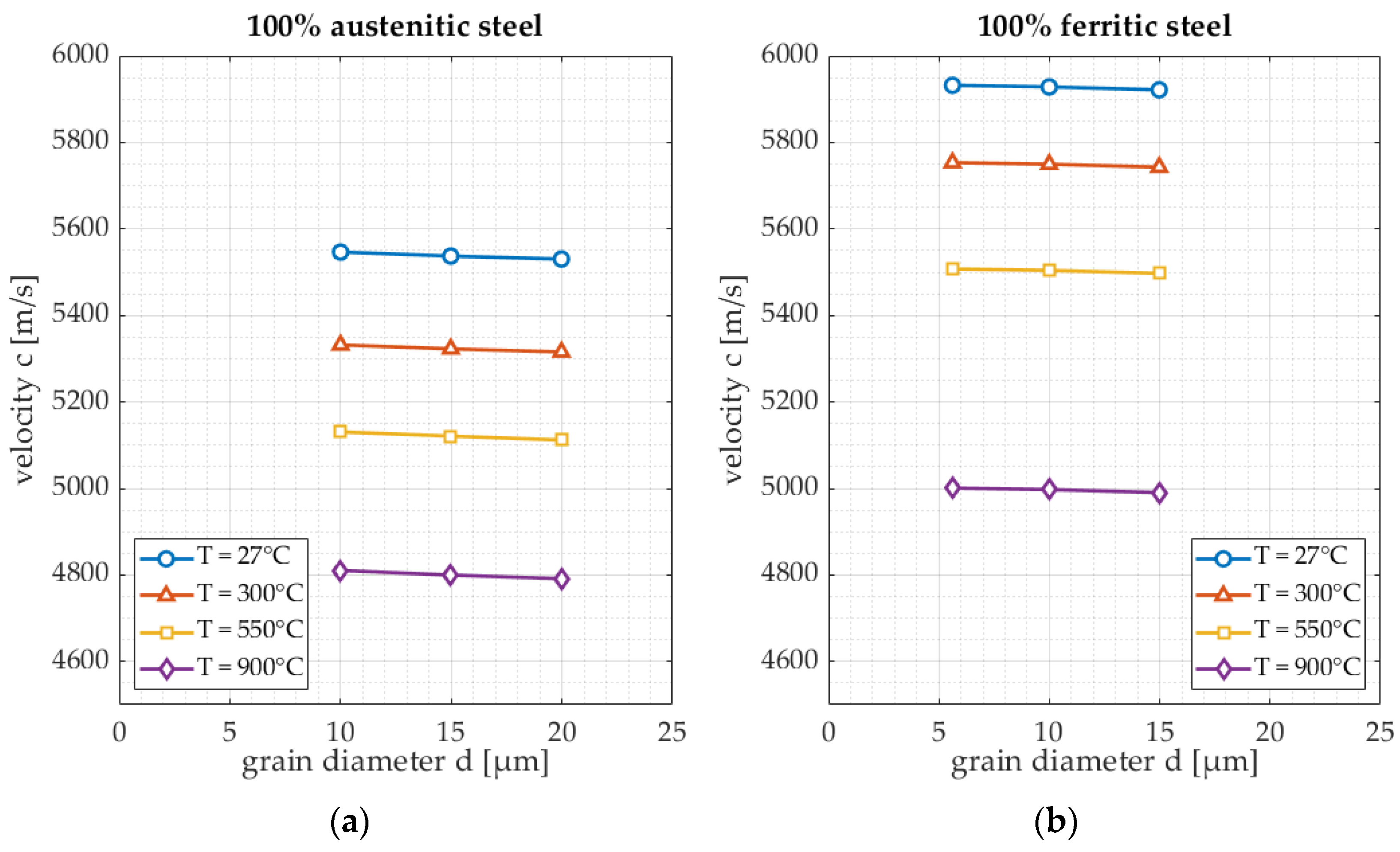
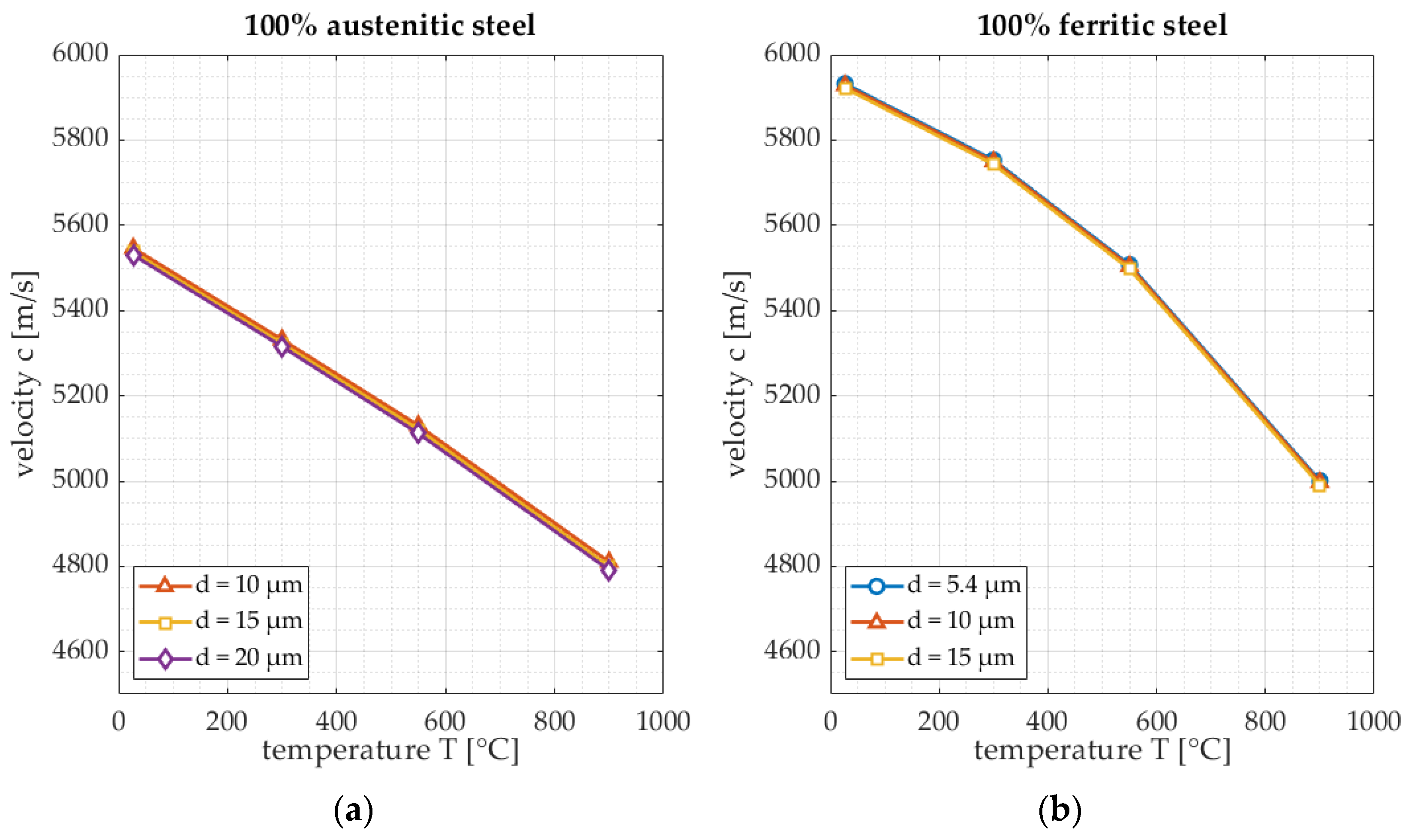
| Microstructure (grain size) Reference points: Austenite: 15 µm Ferrite: 10 µm | Austenite: velocity decrease of 1.6 m/s per µm. Ferrite: velocity decrease of 1.1 m/s per µm. | Austenite: attenuation increase of 0.03 per µm. Ferrite: attenuation increase of 0.011 per µm. |
| Phase volume fraction (austenite/martensite) Reference point: fraction of 50%/50% | Velocity increase of 37 m/s per 10 percent increase of the martensite fraction. | Attenuation increase of 0.02 per 10 percent increase of the martensite fraction. |
| Sample Characteristic | Measurement | Temperature Accuracy | Thickness Accuracy |
|---|---|---|---|
| Microstructure (grain size) 1 µm accuracy | Velocity | Austenite: 2 °C Ferrite: 1 °C | Austenite: less than 10 µm Ferrite: less than 10 µm |
| Attenuation | Austenite: 100 °C Ferrite: 100 °C | - | |
| Phase volume fraction 10% accuracy | Velocity | 50 °C | In the order of 20 µm |
| Attenuation | 70 °C | - |
Disclaimer/Publisher’s Note: The statements, opinions and data contained in all publications are solely those of the individual author(s) and contributor(s) and not of MDPI and/or the editor(s). MDPI and/or the editor(s) disclaim responsibility for any injury to people or property resulting from any ideas, methods, instructions or products referred to in the content. |
© 2023 by the authors. Licensee MDPI, Basel, Switzerland. This article is an open access article distributed under the terms and conditions of the Creative Commons Attribution (CC BY) license (https://creativecommons.org/licenses/by/4.0/).
Share and Cite
Duijster, A.; Volker, A.; Van den Berg, F.; Celada-Casero, C. Estimation of Grain Size and Composition in Steel Using Laser UltraSonics Simulations at Different Temperatures. Appl. Sci. 2023, 13, 1121. https://doi.org/10.3390/app13021121
Duijster A, Volker A, Van den Berg F, Celada-Casero C. Estimation of Grain Size and Composition in Steel Using Laser UltraSonics Simulations at Different Temperatures. Applied Sciences. 2023; 13(2):1121. https://doi.org/10.3390/app13021121
Chicago/Turabian StyleDuijster, Arno, Arno Volker, Frenk Van den Berg, and Carola Celada-Casero. 2023. "Estimation of Grain Size and Composition in Steel Using Laser UltraSonics Simulations at Different Temperatures" Applied Sciences 13, no. 2: 1121. https://doi.org/10.3390/app13021121
APA StyleDuijster, A., Volker, A., Van den Berg, F., & Celada-Casero, C. (2023). Estimation of Grain Size and Composition in Steel Using Laser UltraSonics Simulations at Different Temperatures. Applied Sciences, 13(2), 1121. https://doi.org/10.3390/app13021121