Article

A Feasibility Study for a Hand-Held Acoustic Imaging Camera

1
DiSEGIM—Department of Economics, Law, Cybersecurity, and Sports Sciences, Università Degli Studi di Napoli Parthenope, Via Guglielmo Pepe, 80035 Nola, Italy
2
DIBRIS—Department of Informatics, Bioengineering, Robotics and Systems Engineering, Università Degli Studi di Genova, Via Dodecaneso 35, 16146 Genova, Italy
Appl. Sci. 2023, 13(19), 11110; https://doi.org/10.3390/app131911110
Submission received: 15 June 2023 / Revised: 7 September 2023 / Accepted: 4 October 2023 / Published: 9 October 2023
(This article belongs to the Special Issue New Advances in Audio Signal Processing)

Abstract

:
Acoustic imaging systems construct spatial maps of sound sources and have potential in various applications, but large, cumbersome form factors limit their adoption. This paper investigates methodologies to miniaturize acoustic camera systems for improved mobility. Our approach optimizes planar microphone array design to achieve directional sensing capabilities on significantly reduced footprints compared to benchmarks. The current prototype utilizes a 128−microphone, 50 × 50 cm2 array with beamforming algorithms to visualize acoustic fields in real time but its stationary bulk hampers portability. We propose minimizing the physical aperture by carefully selecting microphone positions and quantities with tailored spatial filter synthesis. This irregular array geometry concentrates sensitivity toward target directions while avoiding aliasing artefacts. Simulations demonstrate a 32−element, ≈20 × 20 cm2 array optimized this way can outperform the previous array in directivity and noise suppression in a sub-range of frequencies below 4 kHz, supporting a 4× surface factor reduction with acceptable trade-offs. Ongoing work involves building and testing miniature arrays to validate performance predictions and address hardware challenges. The improved mobility of compact acoustic cameras could expand applications in car monitoring, urban noise mapping and other industrial fields limited by current large systems.

1. Introduction

Acoustic imaging is an emerging methodology that aims to create spatial maps of sound sources analogous to conventional optical cameras. It digitally reconstructs acoustic fields based on the analysis of sound waves captured by microphone arrays and advanced signal processing algorithms [1,2]. Well-known and widespread acoustic imaging applications include sonar and ultrasound [3]. Potential applications include pinpointing mechanical faults in machines [4], monitoring transport noise pollution [5], locating sniper fire in combat zones [6], validating room acoustics models [7], and many others spanning industrial inspection, public health, security, and virtual reality domains. While optical cameras form images along physical sight lines, acoustic cameras sample sound arriving from diverse directions and computationally focus on particular points in space to create visualizations of sound intensity and origin. This allows passive localization and separation of multiple simultaneous sources based on spatial diversity. The core signal processing operation is known as beamforming, which applies carefully engineered delays and filters to the microphone signals to isolate particular propagation directions [3]. However, performance is subject to physical constraints and trade-offs inherent to the microphone array design [2,8]. In particular, existing real-time acoustic imaging systems utilize large multi-microphone apertures to achieve sufficient angular resolution and sensitivity [9].
This leads to bulky configurations unsuitable for portable applications with limited size, weight, and power budgets (see for instance https://www.flir.com/browse/industrial/acoustic-imaging-cameras/, accessed on 14 June 2023). There is strong motivation to miniaturize such cameras for more accessible and more extensive deployment. This paper investigates methodologies to reduce the form factor of real-time acoustic imaging systems by an order of magnitude while minimizing losses in spatial filtering fidelity. We specifically consider the case study of the Dual Cam (Figure 1), an acoustic camera prototype developed at the Italian Institute of Technology [10]. It combines a 0.5 × 0.5 m2, 128−element microphone array with an embedded system for real-time beamforming and visualization over wideband [500, 6400] Hz. While high-performing, the large stationary apparatus restricts usage scenarios. Our approach is to co-optimize the array configuration and beamforming filters through simulations to retain directional acoustic sensing capability on dramatically smaller footprints. We quantitatively demonstrate that a 32−microphone array over a 0.21 × 0.21 m2 aperture optimized for the acoustic frequencies of interest can provide better directivity than the 128−microphone, 0.50 m aperture Dual Cam array from 2 kHz to 6.4 kHz. This supports reducing system size by up to 4× with tolerable imaging trade-offs. Ongoing efforts are focused on constructing miniature microphone arrays guided by these simulations to develop portable acoustic cameras that interface with tablets/laptops and smartphones for easy deployment. Enabling compact, real-time acoustic imaging could expand applications in machine health monitoring where vibration analysis indicates developing faults before catastrophic failure [11], urban noise pollution mapping to improve public health interventions [12], and augmented/virtual reality scene analysis for realistic audio rendering [13,14]. The methodologies and insights presented provide an array of signal processing starting points for researchers and engineers aiming to transform acoustic imaging capabilities from the lab to the field.

2. Acoustic Imaging Concepts

Acoustic imaging seeks to form a spatial map of sound sources in a scene analogous to standard cameras that produce visual images using projected light patterns. Conventional optics passively focus rays along physical lines of sight to reconstruct perspectives. In contrast, acoustic imaging relies on digital sampling, processing, and interpreting acoustic fields using microphone array receivers and beamforming algorithms [15,16]. We provide an overview of fundamental principles including angular resolution, aliasing, array geometry considerations, and beamforming basics.

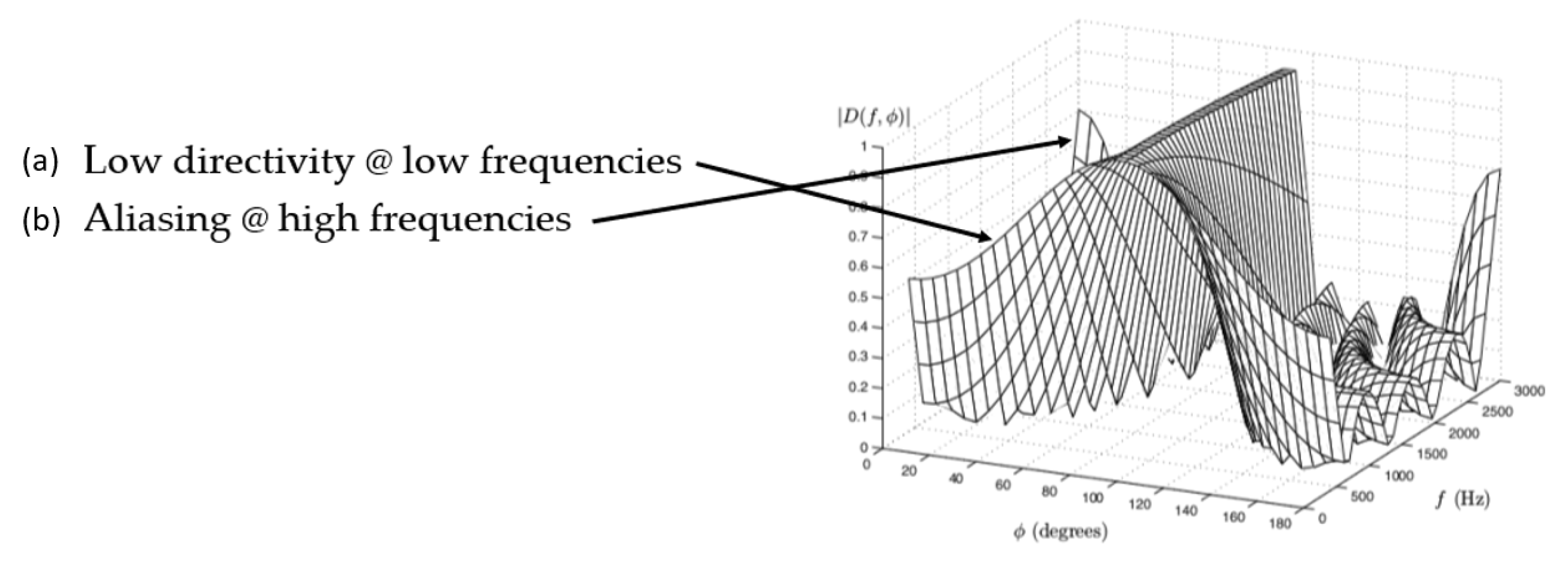
2.1. Angular Resolution

A key parameter in acoustic imaging is the angular resolution, which determines the camera’s ability to spatially discriminate sources [1]. This is influenced by the acoustic wavelength λ , propagation medium sound speed c, and array physical aperture dimensions. The angle θ between two visible sources must satisfy:
θ λ L
where L is the array size normal to the direction of arrival; the constraint arises because waves emitted from within θ will produce signals separated by less than a wavelength, making them indistinguishable. The approximate relationship shows that larger apertures provide finer angular resolution. However, simply using more microphones is insufficient—their positioning is critical, as discussed next.

2.2. Aliasing

The spatial sampling pattern of the microphones can result in aliasing artefacts that distort the acoustic image (Figure 2).
Aliasing occurs when sources at different angular positions generate identical array signals, preventing unique localization. Uniform linear or grid arrays are especially prone due to their periodic sampling structure. Sources separated by multiples of the angular period:
p = sin 1 λ d
where d is the grid spacing, will be aliased since the path length difference between microphones is identical. The resulting grating lobes complicate acoustic imaging by introducing ghost sources and ambiguity. For instance, if we simulate a periodic displacement in a planar array of 25 × 25 cm2 by putting 32 microphones in a regular grid (Figure 3), analysing the beampattern in the window of frequencies [2, 6.4] kHz, we found grating lobes, more evident at higher frequency (Figure 4). A common solution is breaking periodicity by using randomized or aperiodic array layouts [18,19]. However, this must be balanced with microphone density and area coverage to retain sensitivity. Careful array optimization is required to design alias-free configurations suited for imaging.

2.3. Array Geometry

Microphone array geometry plays a critical role in acoustic imaging performance. Key factors are:
  • Aperture —The overall physical size determines angular resolution. Larger apertures improve discrimination.
  • Number of microphones—More microphones provide enhanced spatial sampling at the cost of complexity.
  • Layout—Positions within the aperture area. Uniform grids simplify analysis but suffer aliasing. Randomized arrangements help reduce lobes.
  • Symmetry—Circular/spherical arrays enable uniform coverage but planar designs are easier to manufacture.
The greater the physical dimensions that an array of sensors has compared to what a single transducer allows, with the same wavelength λ considered, the greater the capacity for spatial discrimination of the directions of origin of the signals, and therefore the greater the resolution, referred to in this context as angular resolution. Usually, the dimensions of an array are quantified by evaluating its spatial opening D defined as the maximum distance that separates two elements belonging to it. Therefore, the spatial discrimination capacity of an array coincides with a value proportional to D / λ . An array has properties of flexibility unattainable by the single sensor with the same implementation simplicity. In fact, in many applications, it may be necessary to modify the spatial filtering function in real time to maintain an effective attenuation of the interfering signals to the advantage of the desired ones. This becomes essential in imaging applications in which the pointing direction changes constantly in order to scan all possible directions of arrival of the signal. This change, in a system that adopts an array of transducers, is achieved simply by varying the way in which the beamforming combines the data coming from each sensor in a linear fashion; in the case of a single transducer, the change is impractical as it would be necessary to act directly on the physical characteristics of the sensor.

2.4. Beamforming

Beamforming is the digital signal processing technique that allows microphone arrays to focus on particular directions [20]. It computationally mimics the capability of parabolic dish antennas to isolate radio sources. Delay-and-sum is the simplest beamforming approach. Signals originating from the look direction arrive simultaneously and in phase at the central reference point when appropriately time-shifted. Coherent summation of the aligned microphone signals passes the source undistorted. Off-axis sources remain misaligned, causing attenuation after summing. More advanced optimal and adaptive methods synthesize filters to achieve configurable directional selectivity. The ability to digitally steer the focus point enables scanning to form full acoustic images. Beamforming transforms the microphone array into a highly directional virtual sensor with sensitivity patterns tailored through data-dependent signal processing. However, fundamental limits arise from the array geometry and ambient noise. Robust acoustic imaging requires jointly optimizing the array configuration with advanced beamforming techniques [21,22,23,24] designed to maximize directional resolution.
Ideally, the array would be infinitely large with continuous spatial sampling. In practice, size constraints necessitate designing optimized configurations to maximize imaging capabilities given physical limitations. There are inherent trade-offs between aperture dimensions, microphone density, aliasing artefacts, and processing load that acoustic camera architectures must balance.
The filter-and-sum beamforming algorithm [17,19,25,26,27,28,29,30,31,32,33,34] provides improved performance over the delay-and-sum algorithm by applying filters to the microphone signals. This allows the array to focus on a specific direction more effectively and reduce the sidelobes, resulting in a clearer and more detailed acoustic image.

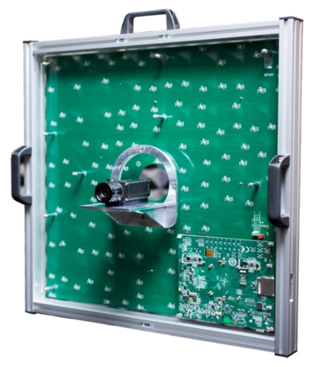
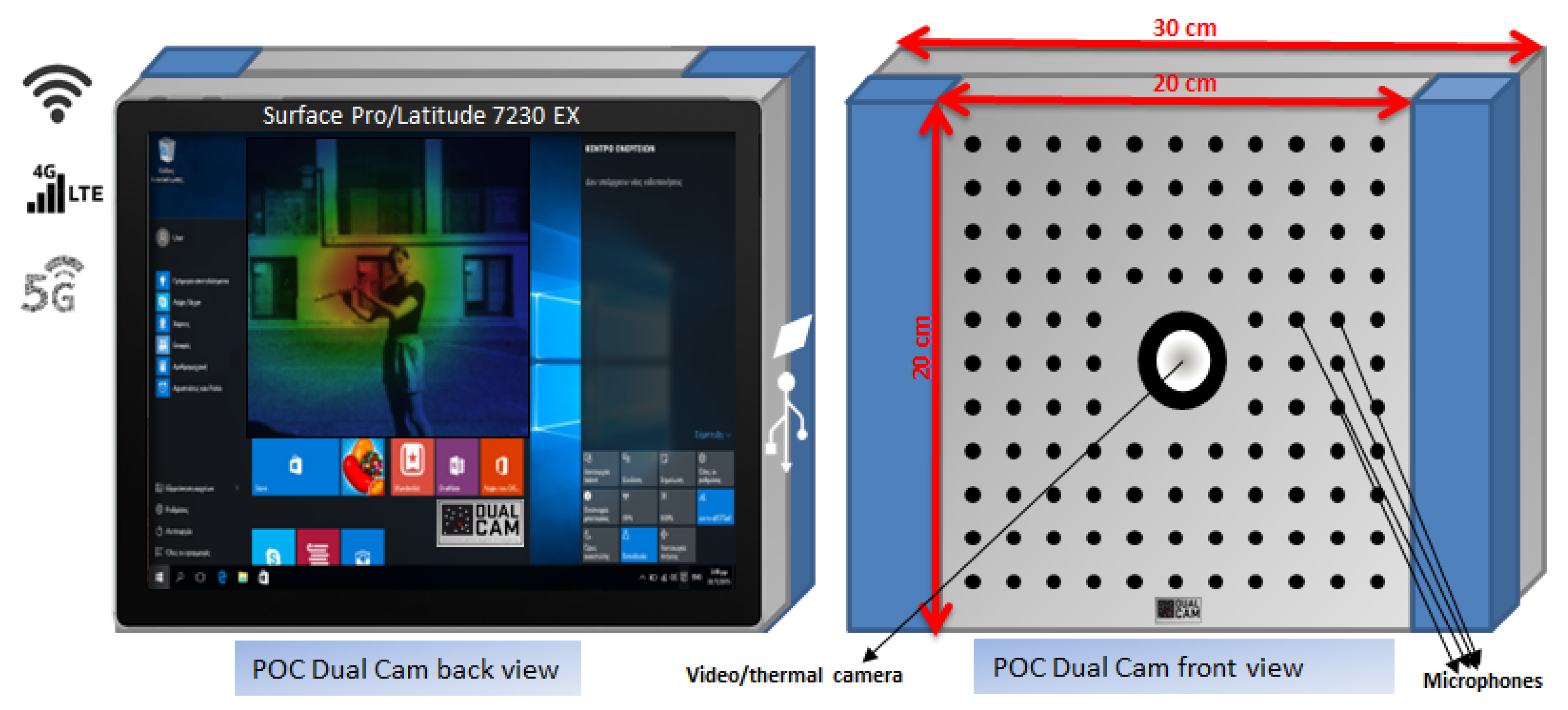
3. Dual Cam Acoustic Camera

We provide an overview of Dual Cam, an acoustic camera prototype developed at the Italian Institute of Technology [10,18]. It combines a co-located planar microphone array and video camera for aligned audiovisual imaging, as illustrated in Figure 1. The current implementation utilizes a 0.5 × 0.5 m2 128−element microphone array fabricated on a custom-printed circuit board working over wideband [500–6400] Hz. Each microphone output is digitized and processed in real time by an embedded system that performs beamforming over an azimuth–elevation scan region, where ( θ , ϕ ) equals (90 × 360) degrees. This generates acoustic images registered to the synchronized video feed, enabling visualization of spatial sound sources. However, the large form factor makes the device cumbersome for portable applications. Our goal is to significantly miniaturize the system while retaining imaging fidelity. Reducing the form factor exacerbates grating lobes and limits low-frequency coverage. Advanced optimization of the layout and beamforming filters is necessary to recover imaging performance on smaller scales through irregular configurations with microphone positioning tailored to the sensors and frequencies of interest.
Acoustic imaging systems utilizing microphone arrays enable novel techniques for localizing and separating multiple simultaneous sound sources. However, real-world deployment remains limited given the unwieldy equipment required. The array’s 128 microphones are strategically positioned using an optimized irregular layout [18,19,35,36,37,38,39] to synthesize directional acoustic images of the sound field when paired with beamforming algorithms [40] (Figure 5). These acoustic images represent spatial auditory information by mapping frequencies to pixels corresponding to locations. While originally high-dimensional, the key acoustic data can be compressed into perceptually relevant mel-frequency cepstral coefficients to reduce computational costs [41] (Figure 5). Studies demonstrate acoustic images can boost model performance by transferring spatial representations to improve audio classification accuracy. The addition of spatial audio details also helps disambiguate sources and generalize to new datasets [42]. However, real-world systems may lack these imaging capabilities. This work examines methodologies to distil the benefits of acoustic images even without access to specialized hardware. Optimized planar arrays provide more accurate spatial audio details compared to individual microphones by sampling sound fields from varied directions. Advanced beamforming techniques enable directionally focused listening to isolate specific sources in noisy scenes. Processing multi-microphone signals remains computationally intensive, though emerging algorithms and parallel computing facilitate real-time performance. The filter-and-sum [3,43] beamformer synthesizes an array of impulse responses to steer directional sensitivity. While specially designed microphone arrays can provide valuable spatial auditory images, this research investigates generalized approaches using array signal processing to improve audio sensing tasks without access to imaging hardware.
The filter-and-sum beamforming algorithm is a method for synthesizing the finite impulse response (FIR) coefficients [17,25,43] for small-sized two-dimensional microphone arrays [19]. This method can be used to generate acoustic images by focusing the array on a specific direction in space and enhancing the signal coming from that direction.
The live acoustic imaging pipeline consists of:
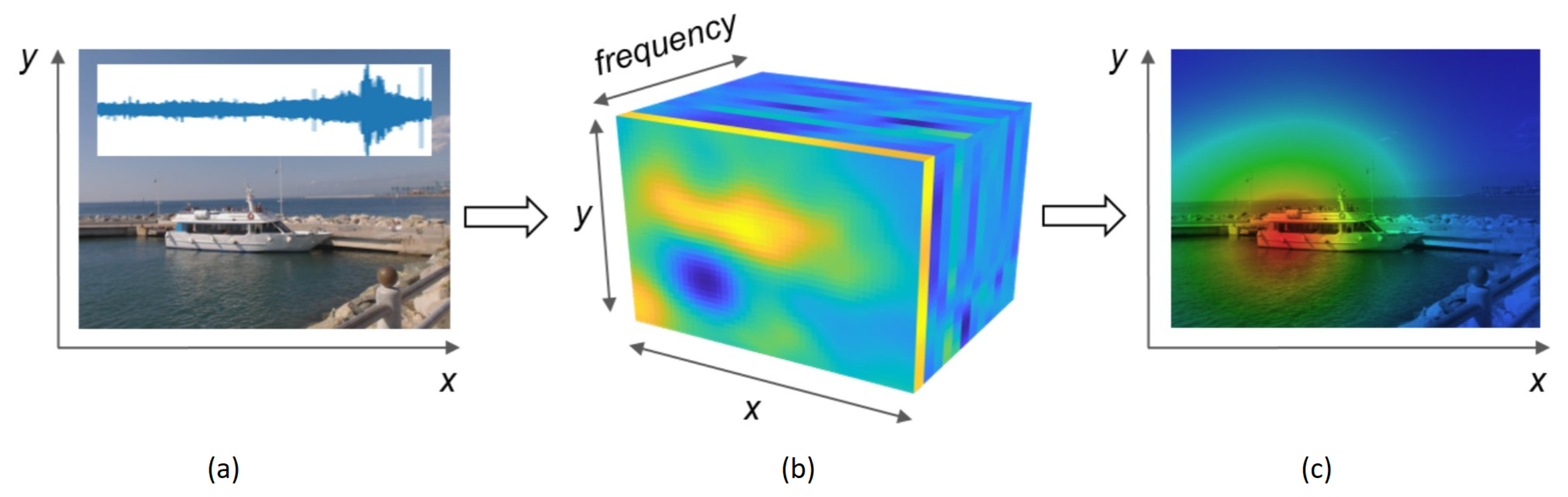
  • Digitizing microphone outputs through multichannel audio sampling.
  • Partitioning the multichannel record into short time frames.
  • Synthesizing beamformer filters according to designed array geometry.
  • Applying filters and aligning signals for each scanning direction.
  • Coherently summing aligned microphone channels to obtain beam pattern power.
  • Repeating overall look directions to generate acoustic image frames registered to video.
This digital signal chain transforms the raw multichannel audio into visualizations of spatial sound intensity (Figure 5 and Figure 6). However, the fidelity is contingent on array configuration, density, and beamforming approach. We investigate techniques to co-optimize these parameters for compact, real-time acoustic cameras without prohibitive degradation compared to larger form factors.

4. Materials and Methods

Recent advancements in acoustic imaging have enabled novel techniques for localizing and separating multiple sound sources within complex auditory scenes. However, current implementations are often constrained to laboratory settings due to large, unwieldy equipment. This research aims to transform an existing prototype (Figure 1) into an engineered portable device for real-world sound source separation (Figure 7). Through compact microphone array design and machine/deep learning algorithms run on a coupled tablet/laptop (for instance Microsoft Surface Pro or Dell Latitude 7230EX) (Figure 8), we can achieve a handheld multimodal camera that captures and processes synchronized audio and video to map multiple simultaneous sounds.
CNNs (convolutional neural networks) frequently employ image classification and segmentation tasks through acoustics. Acoustic images provide automatic learning opportunities for CNNs’ relevant features. Leading CNN structures like ResNet and U-Net have been adopted for acoustic image evaluation. Using RNNs (recurrent neural networks) like LSTMs enables the examination of audio visualization sequences evolving with time. Useful applications exist for monitoring items or procedures within video acoustic microscopy information. Acoustic image denoising and reconstruction are tasks that autoencoders excel at performing. The encoded data enables the decoder to recreate the revitalized picture flawlessly. Using GANs (generative adversarial networks) realistic sound imagery is generated, benefiting data amplification and modelling initiatives. Coordinated development through shared training brings the generator and discriminator closer to perfection. From a historical perspective, these classic ML algorithms—including random forests and support vector machines—continue to serve us well. Manual feature creation makes their training process speedier and more straightforward. Two prominent unsupervised learning approaches—k-means clustering and principal component analysis—assist in identifying hidden patterns within acoustic information. Interactive queries enable users to efficiently annotate crucial data points through active learning techniques. Model selection hinges on parameters like dataset size, work objective, and processing capacity. By investing time and resources into rigorous evaluation, we can create models capable of producing consistent outputs. To retain directional sensitivity in a smaller form factor, we optimize array layouts using analytical filter synthesis and stochastic optimization, assessing robustness via statistical error analysis. Novel steps in our approach are:
  • We optimize the analytic form of the cost function in order to cut the simulation computational load. This optimization of the cost function is a novel contribution beyond the existing state-of-the-art methods, improving computational efficiency.
  • We include the statistical evaluation of the mismatches of the microphones that are more important in shrinking the array size. The statistical characterization of microphone mismatches enables novel array size reduction.
  • We optimize the FOV (field of view) and the frequency bandwidth according to the array size reduction to explore upper harmonic reconstruction to determine whether intelligibility is retained without fundamental frequencies. The joint optimization of FOV, frequency band, and array size reduction using the upper harmonics for intelligibility preservation is an unexplored area representing a novel research direction.
A key goal is extending as much as possible the minimum detectable frequency to improve directivity with fewer elements. While reducing array aperture, we must balance performance trade-offs from decreased low-frequency directivity and potential undersampling artefacts. This work details simulations on irregular aperiodic subsampling to concentrate high-frequency information while avoiding grating lobes (Figure 4) and exploring upper harmonic reconstruction to determine whether intelligibility is retained without fundamental frequencies reducing the device’s bandwidth to optimize the simulation metrics. Following prototype optimization and evaluation using audio test signals, we compare metrics like signal-to-noise ratio to the original large-scale system. This study aims to progress acoustic imaging capabilities from constrained laboratory settings towards real-world applications through engineered mobile platforms. This work aims to re-engineer a compact, portable prototype (Figure 7) that transmits synchronized audio and video data streams to a commercial tablet or laptop. The audio is captured by an array of microphones on the primary module, while the video is acquired by a thermographic or conventional camera. These peripheral modules interface with the central unit via multiple USB connections. Embedding an FPGA onboard the central module alongside an ARM processor enables straightforward interfacing leveraging their integrated architecture (Figure 8). The system operates on battery power with LED indicators and debugging ports and can dock to the tablet mechanically. A remote internet link via WiFi, LTE, or 5G facilitates control and data sharing. The tablet/laptop display provides a visualization interface to process the multimodal data streams using algorithms, machine learning, and deep neural networks. This integrated design retains the core functionality of the original laboratory prototype while minimizing size and maximizing portability for real-world deployment. Ongoing work focuses on implementation challenges including power optimization, heat dissipation, enclosure design, calibration, and field testing. By progressing acoustic imaging capabilities from constrained lab settings to handheld adaptable platforms, this research aims to unlock new applications in machine condition monitoring, spatial sound mapping, and other domains limited by current large-scale wired systems.

5. Array Optimization Methodology

Reducing the physical array aperture while maintaining usable imaging resolution requires balancing size, microphone number, spatial sampling, and angular coverage. Simply downscaling a regular grid array would significantly increase grating lobes (Figure 4 and Figure 9). We instead utilize array signal processing optimization procedures that allow unconventional configurations with microphone numbers and positions tailored to imaging requirements. Irregular layouts are synthesized based on maximizing acoustic power focused toward directions of interest and minimizing ghost images. Key concepts are briefly introduced below (Figure 9), with formulations adapted from [8,18,35].

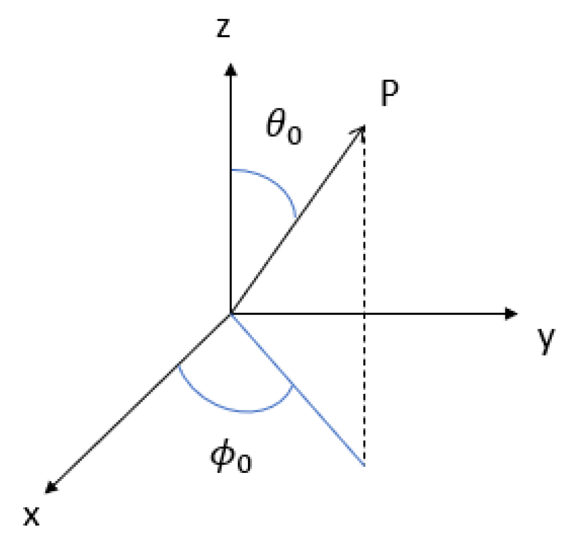
5.1. Problem Parameterization

We consider a planar array of N microphones located at positions r n = ( x n , y n ) in the x y plane (Figure 10). Acoustic sources at frequency f impinge on the array from angles θ and ϕ . The goal is to generate high-resolution, low-artefact acoustic images over the signal band [ f min , f max ] . The array geometry and frequency-dependent beamformer filter coefficients w ( f ) = [ w 1 ( f ) , , w N ( f ) ] T are jointly optimized to maximize directional sensitivity. The complex beam pattern B ( θ , ϕ , f ) encodes the array response at each look angle and is parameterized as:
B ( θ , ϕ , f ) = n = 1 N w n ( f ) e j 2 π f r ^ ( θ , ϕ ) · r n
where r ^ ( θ , ϕ ) is the source position unit vector. The expression depends on both the layout r n and filter coefficients w n ( f ) which are microphone-specific filters to be optimized. The expression has directionality dependence on both the layout r n and filter responses w n ( f ) . To allow joint optimization, a cost function J ( w , r ) is formulated that balances simultaneously directional focus, artefact suppression, frequency coverage, and robustness. It incorporates an idealized unity gain beampattern B 0 ( θ , ϕ , f ) at the look direction and minimizes the deviation from this response over angle-frequency space. Regularization terms manage overall beamformer gain and robustness. The optimization determines array configurations and filters customized for the imaging application. With the beam pattern expressed as B ( θ , ϕ , f ) = w T ( f ) V ( θ , ϕ ) , the filter coefficients w ( f ) can be analytically extracted from the cost function into a closed-form solution w opt ( f ) = R 1 ( f ) q ( f ) . For the array layout optimization with w opt ( f ) fixed, simulated annealing avoids poor local minima. Iterative stochastic perturbations to microphone locations r n are accepted probabilistically based on the cost function to enable escaping local minima. After sufficient iterations, the array geometry converges to enhance directionality. To improve robustness, the cost function is averaged over possible microphone gain and phase errors modelled as random variables. This penalizes configurations with low white noise gain, minimizing sensitivity to imperfections. The expected beam pattern E [ B ( θ , ϕ , f ) ] is incorporated to account for errors; this optimization framework (Figure 9) allows the designing of array geometries and filters customized for compact, robust acoustic imaging over desired frequency bands. The resulting unconventional configurations maximize power focused on look directions while minimizing off-axis contributions and artefacts using small apertures.
The cost function J ( w , r ) balances several competing objectives:
  • Directional focus. Minimizing deviation of the achieved beam pattern B ( θ , ϕ , f ) from the ideal unity gain pattern B 0 ( θ , ϕ , f ) at the look direction over angle-frequency space. This is quantified by the integral term:
    Θ , Φ , F | B ( θ , ϕ , f ) B 0 ( θ , ϕ , f ) | 2 d θ d ϕ d f
  • Artefact suppression. Minimizing the beam pattern gain away from the look direction, incorporated through:
    Θ , Φ , F | B ( θ , ϕ , f ) | 2 d θ d ϕ d f
  • Frequency coverage. Optimizing over the full band [fmin, fmax] through integration over f.
  • Robustness. Averaging over microphone imperfections by modelling gain and phase as random variables A n .
The overall form is a weighted combination of these terms:
J ( w , r ) = α | B ( θ , ϕ , f ) B 0 ( θ , ϕ , f ) | 2 d θ d ϕ d f + ( 1 α ) | B ( θ , ϕ , f ) | 2 d θ d ϕ d f
where α [ 0 , 1 ] controls the trade-off between directional focus and artefact suppression. To minimize J, the filter coefficients w ( f ) are first optimized analytically for a fixed array layout by extracting them into a quadratic form with closed-form solution w opt ( f ) .
The microphone locations r n are then optimized stochastically using simulated annealing to avoid poor local minima:
  • Iterative random perturbations Δ r n are applied to the microphone locations.
  • New locations are accepted probabilistically based on the cost J.
  • Acceptance probability is higher at higher initial “temperatures” and cooled over iterations.
  • After sufficient iterations, r n converges to a geometry minimizing J.
This joint optimization determines array layouts and filters tailored for directional imaging over the specified band with artefact suppression and robustness. In the simulation of the beampattern of a planar array ( z = 0 ) of microphones we have two angles of arrival θ and ϕ , two steering angles θ 0 and ϕ 0 (Figure 10) and two coordinates for the microphones x n and y n . The mathematical expression of the ideal superdirective beampattern B in far-field is:
B ( θ , ϕ , θ 0 , ϕ 0 , f ) = n = 1 N w n ( f ) e j 2 π f · x n · sin ( θ ) sin θ 0 c + y n · sin ( φ ) sin φ 0 c
where N is the number of microphones, c = 340 m/s is the speed of the acoustic waves into the medium ( λ = c / f ), and w n ( f ) is the frequency response of the n-th filter:
w n ( f ) = k = 1 K w n , k · e j 2 π f · k T c

5.2. Cost Function Definition

We recall the cost function formulated to allow optimizing the array layout and beamformer filters for directional acoustic imaging:
J ( w , r ) = α Θ , Φ , F B ( θ , ϕ , f ) B 0 ( θ , ϕ , f ) 2 d θ d ϕ d f + ( 1 α ) Θ , Φ , F B ( θ , ϕ , f ) 2 d θ d ϕ d f
B 0 ( θ , ϕ , f ) is the idealized beam pattern with unity gain at the main look direction and zero elsewhere. The first term drives the achieved response toward the desired spatial selectivity. The second term balances overall beamformer gain and robustness. α [ 0 , 1 ] controls the trade-off. The integrals are approximated over discrete grids of angles and frequencies. This cost function steers the optimization toward arrays with high directionality for acoustic imaging. It encapsulates the desired balance of sharp focus, minimal artefacts, wide frequency coverage, and robustness within a single numerical measure of performance. In order to find the position of the microphones, we have to minimize the J cost function [18] that we rewrite as:
J ( w , r ) = θ 0 min θ 0 max ϕ 0 min ϕ 0 max θ min θ max ϕ min ϕ max f min f max B w , r , θ , ϕ , θ 0 , φ 0 , f 1 2 + C B w , r , θ , ϕ , θ 0 , ϕ 0 , f 2 d θ d ϕ d θ 0 d ϕ 0 d f
where r is the vector with the positions of the microphones, w is the vector of the filter coefficients, and C is a real constant. This tunes the minimization of the first term of the cost function which is the adherenceterm and the second one which is the energy weighted term. We want to joint optimization of weights and microphones’ positions and account for superdirectivity and aperiodicity. Then, the expression (4) of the beampattern B of a planar array ( z = 0 ) of microphones in 2−D becomes:
B w , r , θ 0 , ϕ 0 , θ , ϕ , f = n = 1 N k = 1 K w n , k e j 2 π f · x n sin ( θ ) sin θ 0 c + y n · sin ( ϕ ) sin ϕ 0 c + k T c
where K is the length of the FIR filter and T c is the sampling period.

5.3. Directivity Optimization

The beam pattern expression can be reduced to:
B ( θ , ϕ , f ) = w T ( f ) V ( θ , ϕ )
where w ( f ) = [ w 1 ( f ) , , w N ( f ) ] T and V ( θ , ϕ ) is an array manifold vector with phase terms dependent on look direction. This allows extracting the filter coefficients from the cost function, converting optimization over w ( f ) into a quadratic form with a closed-form solution:
w o p t ( f ) = R 1 ( f ) q ( f )
where R ( f ) and q ( f ) accumulate integration terms. The optimal w o p t ( f ) maximizes directionality for a given layout.

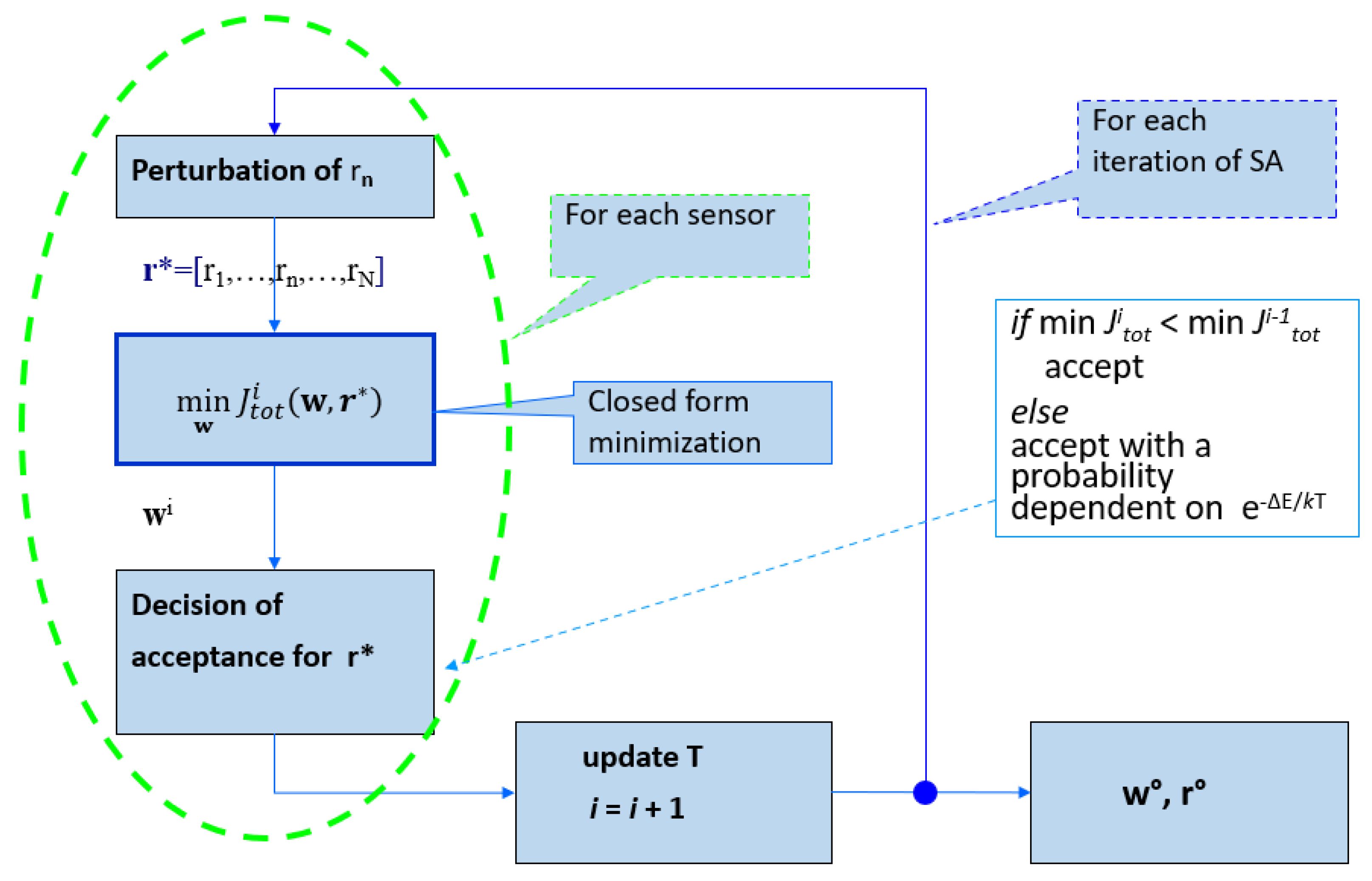
5.4. Layout Optimization

In order to achieve and improve robustness against microphone imperfections, we perform an optimization of the mean performance i.e., the multiple integrals of the cost function over the sensors’ phase e γ n and gain a n A n = a n · e γ n considered as random variables, getting a robust cost function with the PDF (probability density function) of the random variable A n [38]. The cost function J ( w , r ) is averaged over possible gain and phase errors by modelling the microphone responses A n as random variables:
J tot ( w , r ) = A 0 A N 1 J ( w , r , A 0 , , A N 1 ) f A ( A 0 ) f A ( A N 1 ) d A 0 d A N 1
where f A ( A n ) is the PDF of the random variable A n . This incorporates robustness into the optimization. However, evaluating the multiple integrals results in a large number of variables (microphone positions and FIR filter coefficients) making direct optimization of J tot computationally infeasible. To address this, a change of variables is made:
u = sin ( θ ) sin θ 0 v = sin ( ϕ ) sin ϕ 0
Substituting into the beam pattern expression gives:
B ( w , r , u , v , f ) = n = 1 N k = 1 K w n , k e j 2 π f ( x n u c + y n v c + k T c )
This allows for defining a simplified cost function:
J tot ( w , r ) = u min u max v min v max f min f max | B ( w , r , u , v , f ) 1 | 2 + C | B ( w , r , u , v , f ) | 2 d f d u d v
The filter coefficients w can then be analytically extracted into a quadratic form with a closed-form solution:
J tot ( w , r ) = w T M w 2 w T r + s
Further, the robustness integrals over A n can be approximated in closed form. The microphone positions r n are then numerically optimized using simulated annealing to avoid local minima. Iterative stochastic perturbations escape suboptimal configurations based on the cost. This joint optimization determines robust array geometries and filters for directional imaging. Performance is evaluated using metrics such as directivity D ( f ) and white noise gain W N G ( f ) . The expected beam pattern power E { | B ( θ , ϕ , f ) | 2 } is also incorporated to account for microphone imperfections. Minimizing tolerance to errors improves reliability. This framework enables the designing of robust, compact arrays tailored for spatial acoustic imaging over desired bands. The new cost function is a good approximation of the original one, allowing the number of integrals to be reduced. The vector w can be extracted from the multiple integrals in the robust cost function obtaining a quadratic form in w [18]. With ideal filters derived analytically, the microphone locations r n are optimized stochastically. A simulated annealing approach is used to avoid poor local minima. Iterative perturbations to r n are accepted probabilistically based on the cost, allowing escape from local minima at high process “temperatures” that are gradually cooled. After sufficient iterations, the microphone layout converges toward a configuration with scattering tailored to enhance directional sensitivity and suppress off-target responses. The joint optimization determines array geometries and beamformers customized for compact acoustic imaging over specified bands. For a fixed microphone displacement, the global minimum of the robust cost function can be calculated in a closed form. Conversely, the presence of local minima with respect to the microphone position prevents the use of gradient-like iterative methods. The final solution is given by a hybrid strategy analytic and stochastic based on the Simulated Annealing algorithm [36,45] (Figure 11). The steps are:
  • Iterative procedure aimed at minimizing an energy function f ( y ) .
  • At each iteration, a random perturbation is induced in the current state y i .
  • If the new configuration, y * , causes the value of the energy function to decrease, then it is accepted.
  • If y * causes the value of the energy function to increase, it is accepted with a probability dependent on the system temperature, in accordance with the Boltzmann distribution.
  • The temperature is a parameter that is gradually lowered, following the reciprocal of the logarithm of the number of iterations.
  • The higher the temperature, the higher the probability of accepting a perturbation causing a cost increase and of escaping, in this way, from unsatisfactory local minima.

5.5. Robustness Constraints

We require quantitative metrics to evaluate the algorithm’s beamforming performance. The key metrics utilized are the frequency-dependent directivity D ( f ) and white noise gain W N G ( f ) , computed for steering angles θ 0 and ϕ 0 . For a planar array, the directivity (in dB) is defined as:
D ( f ) = | B ( θ 0 , ϕ 0 , f ) | 2 1 4 π 0 2 π 0 π | B ( θ , ϕ , f ) | 2 sin ( θ ) d θ d ϕ
The white noise gain (in dB) quantifies robustness towards array imperfections:
W N G ( f ) = | B ( θ 0 , ϕ 0 , f ) | 2 n = 1 N | w n ( f ) | 2
We propose the expected beam pattern power (EBPP) metric to statistically evaluate the impact of variance in array gain and phase on the beam pattern B ( f ) :
B e 2 ( θ , ϕ , f ) = E | B ( θ , ϕ , f ) | 2 = A 0 A N 1 | B ( θ , ϕ , f ) | 2 · f A 0 ( A 0 ) f A N 1 ( A N 1 ) d A 0 d A N 1
Microphone imperfections can distort the array away from the ideal modelled response. As in [38], robustness is incorporated by averaging the cost function over possible gain and phase errors through the expectation operator E { . } .
E [ B ( θ , ϕ , f ) ] | B ( θ , ϕ , f ) | 2 + 1 W N G ( f ) ( σ g 2 + σ ψ 2 )
where σ g 2 and σ ψ 2 are variances of normally distributed microphone magnitude and phase mismatches, and W N G ( f ) is a white noise gain term. Minimizing cost tolerance to modelled errors helps ensure reliable performance. This full optimization framework allows the designing of microphone array geometries and beamformers customized for compact acoustic imaging over desired signal bands. The unconventional configurations maximize power focused toward look directions while suppressing artefacts and minimizing off-axis contributions to enable resolving spatial sound fields from small apertures. We next utilize this approach in a simulation case study of miniature array optimization. With the proposed metrics in place, we evaluate the directivity D ( f ) , white noise gain W N G ( f ) , and expected beam pattern power (EBPP) for our initial simulated array design. We model the microphone mismatches as Gaussian distributions with σ g = 0.03 = 3 % for gain error and σ ψ = 0.035 rad 2 for phase error. This preliminary simulation provides favourable results across the three figures of merit, indicating promising performance in reshaping the sensor array for the Dual Cam 2.0 system. The directivity quantifies the main lobe sharpness, white noise gain captures robustness, and the expected beam pattern incorporates statistical variations—together assessing the shaped array’s directional sensitivity, imperfections tolerance, and expected real-world behaviour. Further refinements to the array geometry and element tuning will build upon these initial positive findings, working toward an optimal miniature microphone configuration.

6. Simulation Configuration

We implement the array optimization procedures in MATLAB to enable rapid evaluation of miniaturized acoustic camera designs. The custom cost function represents the mismatch between achieved and ideal beampatterns over angles Θ , Φ and frequencies F = [ 0.5 , 6.4 ] kHz. At each iteration, filter coefficients are computed analytically then microphone positions are perturbed stochastically to minimize artefacts. The optimization concentrates power within a ± 20 degree main lobe while suppressing sidelobes. Array performance is assessed by analysing:
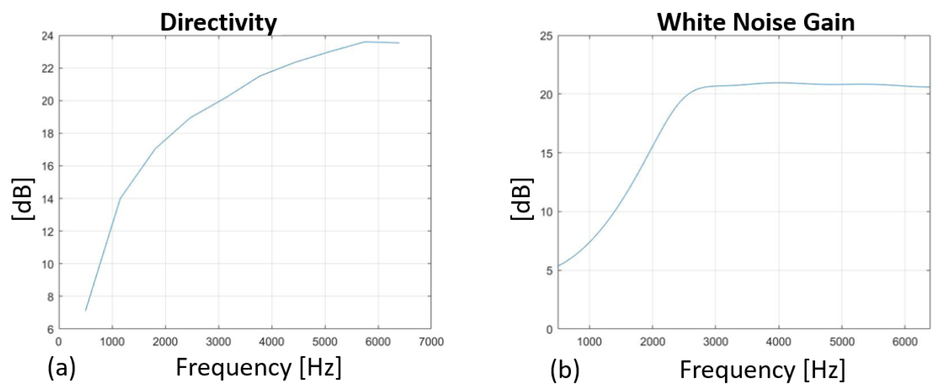
  • Directivity—angular discrimination capability;
  • White noise gain (WNG)—robustness to fabrication variations;
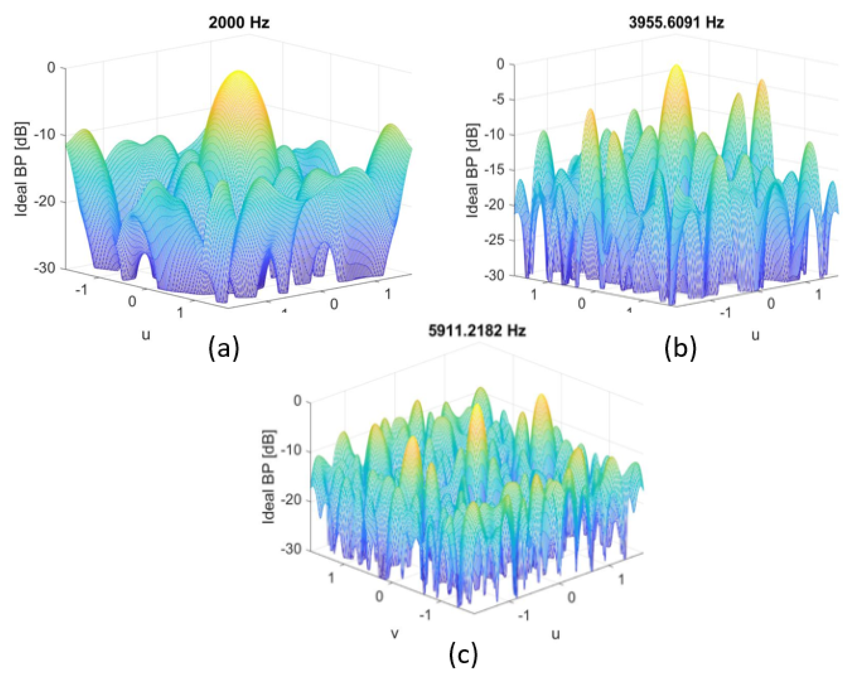
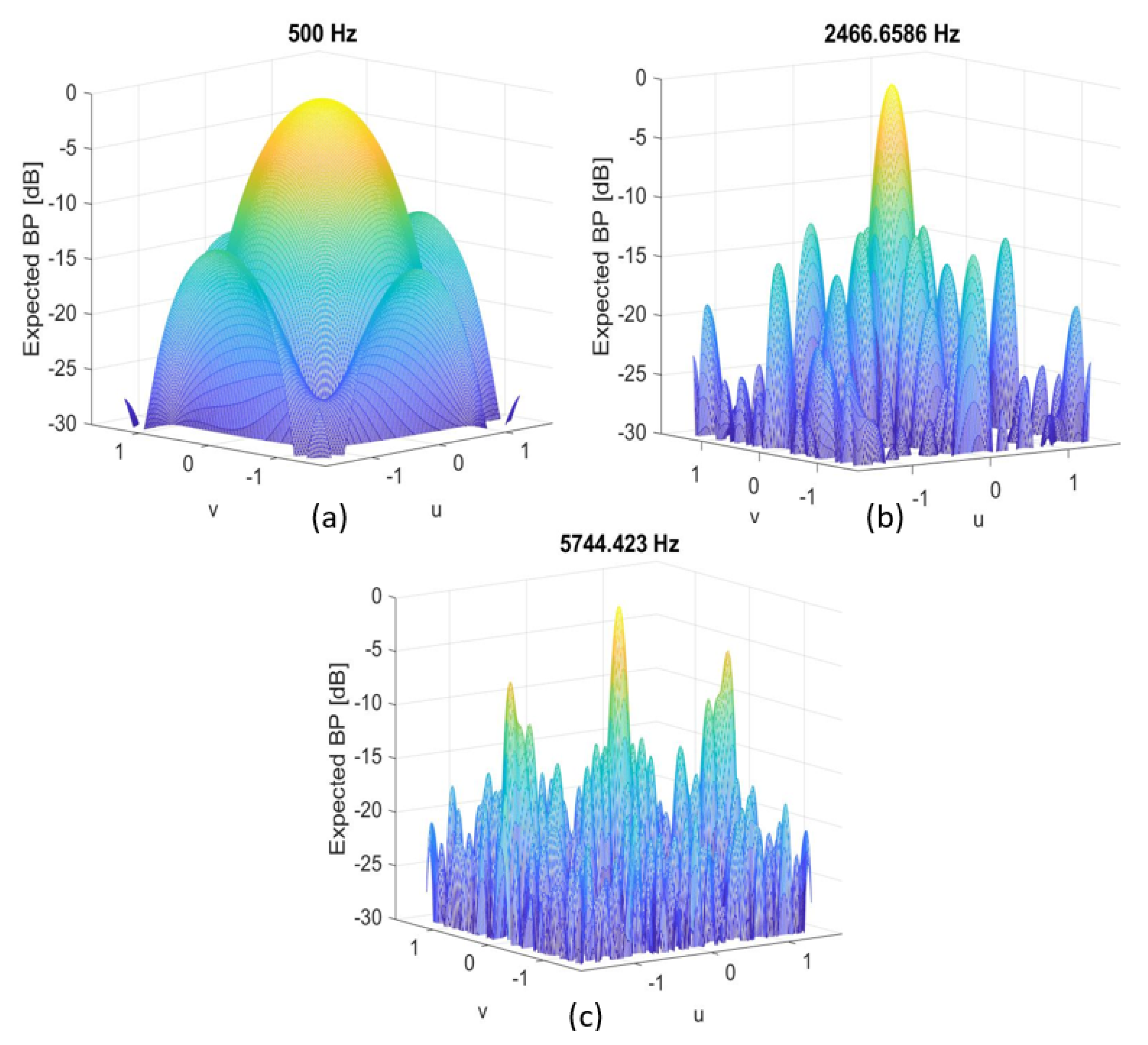
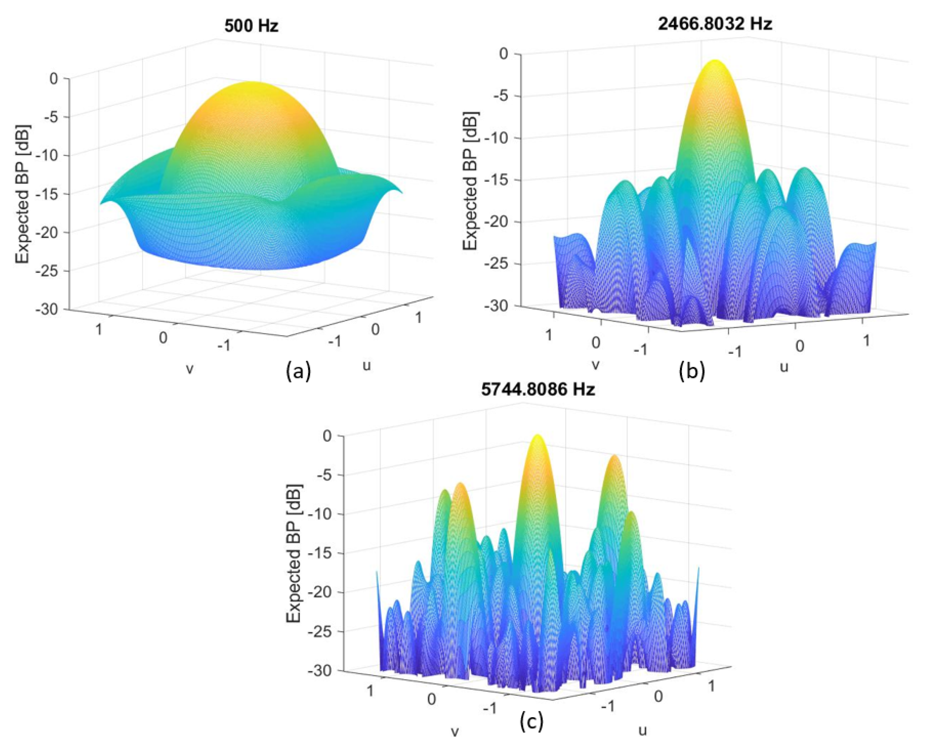
  • Beam patterns and sidelobe levels—imaging artefacts.
The numerical approach allows for efficient simulation of miniaturized configurations to quantify expected imaging performance and determine plausible hardware parameters. We consider three scenarios:
  • A 32−microphone 0.25 m square array optimized from 2 to 6.4 kHz.
  • A 32−microphone 0.21 m square array optimized from 2 to 6.4 kHz.
  • A 32−microphone 0.21 m square array covering [0.5, 6.4] kHz for comparison with Dual Cam specifications (128−microphone on a 0.5 m square array).
The different number of microphones and expanded frequency range in Case 3 demonstrates trading off aperture size versus density given constraints. Comparisons with a modelled 128−element 0.5 m array representing Dual Cam provide context on expected miniaturization imaging trade-offs. The simulation results guide physical prototype development by predicting achievable performance bounds with compact arrays.

7. Miniaturized Array Optimization: Results and Discussion

We present synthesized array configurations from the three simulated case studies along with an analysis of beam patterns, directivity, and white noise gain for Dual Cam 2.0.

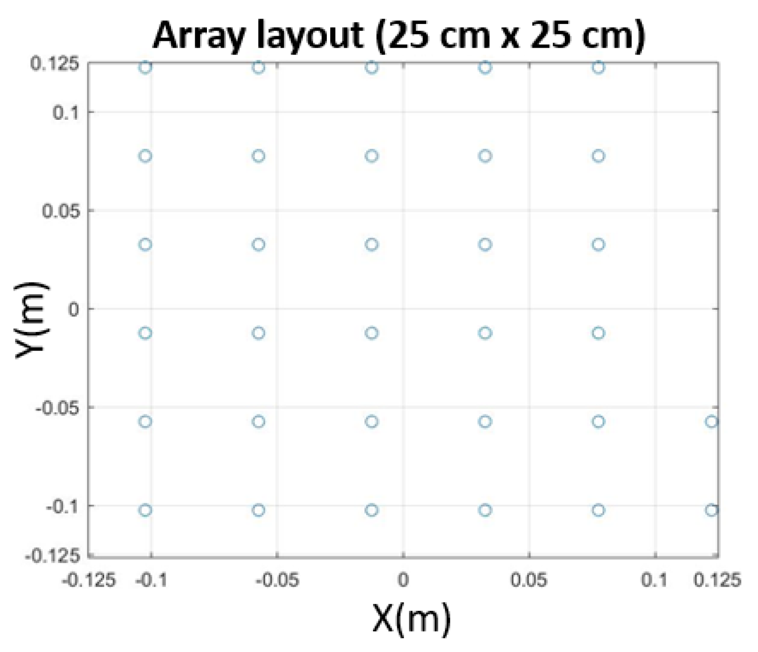
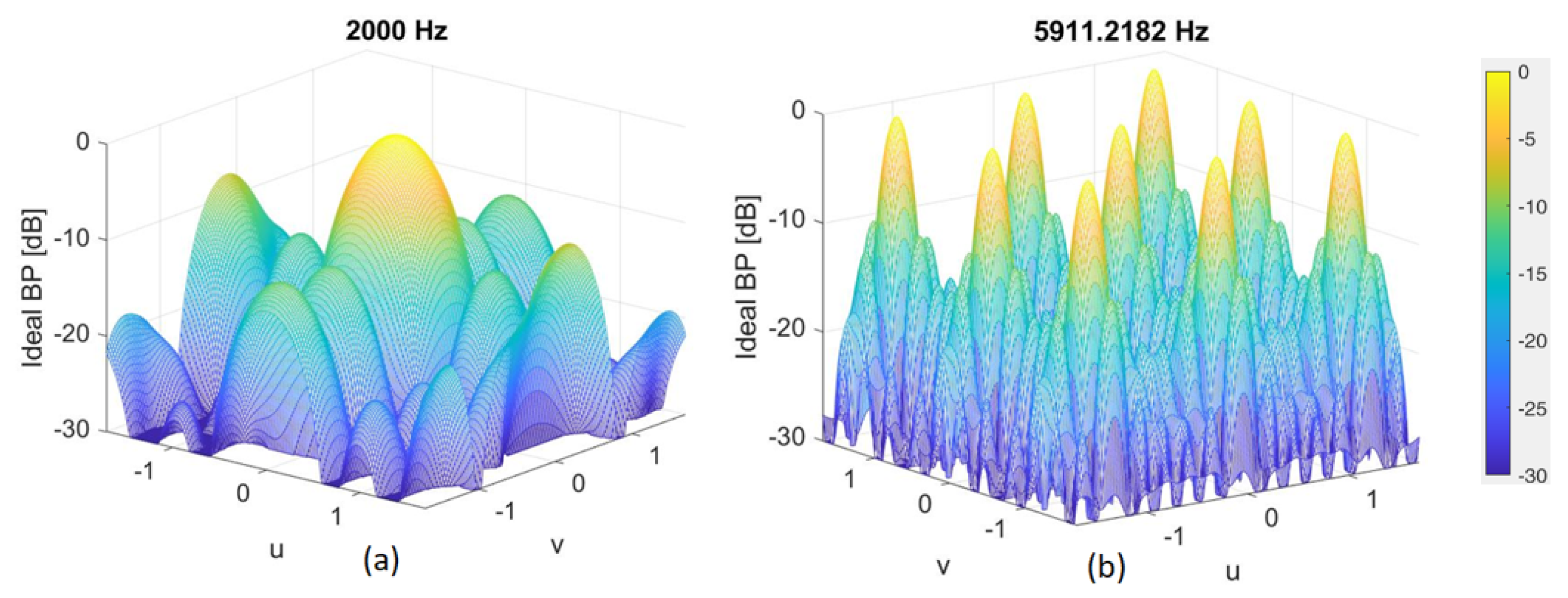
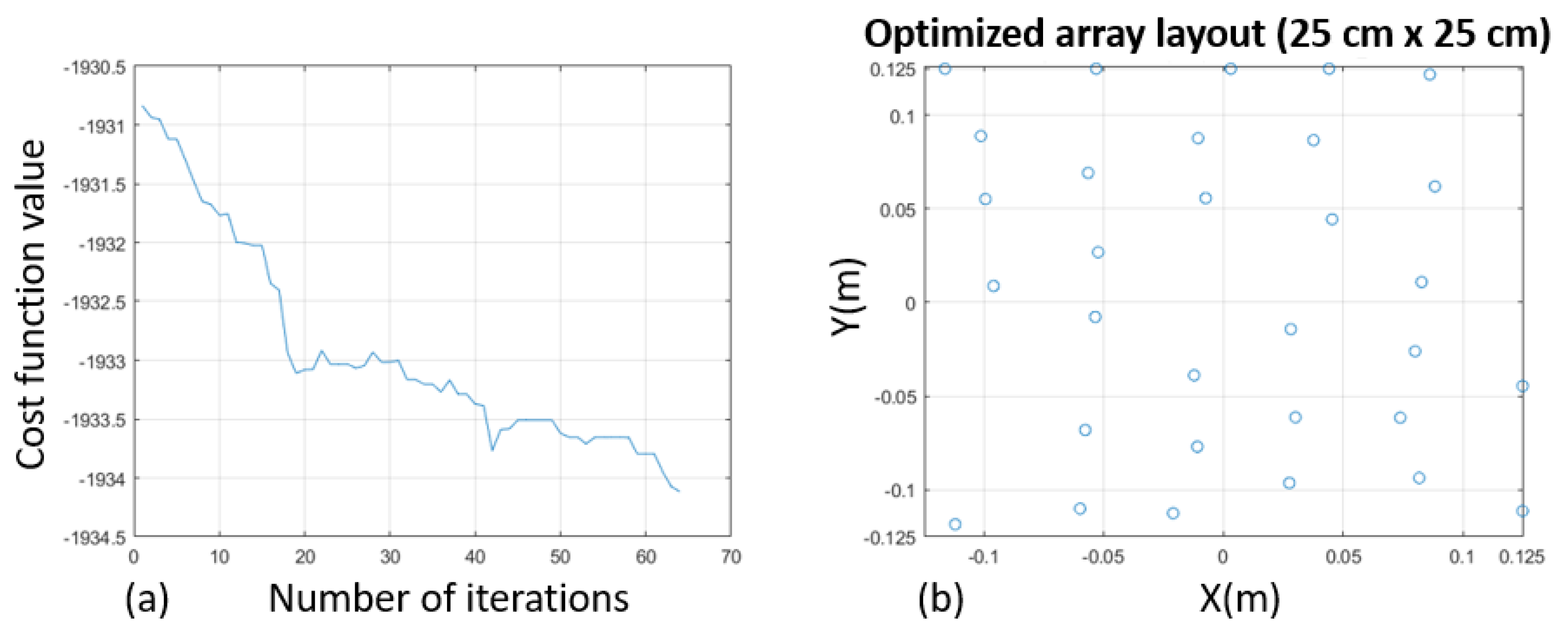
7.1. Thirty-Two-Microphones, [2, 6.4] kHz, Array 25 × 25 cm2

The first scenario optimizes a 0.25 × 0.25 m2 32−microphone array for a 4.4 kHz bandwidth. After 100 iterations, the cost function converges as shown in Figure 12. The corresponding irregular array geometry has an aperiodic structure with variable microphone spacing tailored for the acoustic parameters.
We tried to reduce the planar array aperture (u and v range) to adjust the FOV (field of view) and to increase the number of iterations. We tested this full setting:
  • L = 25 cm;
  • of microphones = 32 mic;
  • K = 31 (FIR length);
  • u ∈ [−1. 5; 1.5];
  • v ∈ [−1.5; 1.5];
  • of iterations = 100;
  • Bandwidth = [2000, 6400] Hz.
As expected, low-frequency performance is improved relative to the bandwidth [2, 6.4] kHz 32−elements array. The directivity comparison (Figure 13a) with a 0.21 × 0.21 m2 prototype in the bandwidth [0.5, 6.4] kHz indicates better sensitivity below 4 kHz. This demonstrates the potential for substantial miniaturization through optimization over the frequency bandwidth. The 32−microphone design retains 15 dB (Figure 13b) robustness, with improved low-frequency gains offsetting minor high-frequency trade-offs. The beam patterns in Figure 14 verify directional selectivity and sidelobe suppression within the band.
The beam patterns in Figure 14 show low sidelobes within the band. However, some aliasing emerges at higher frequencies due to the reduced aperture size. The 10 dB directivity in Figure 13a confirms directional sensitivity is retained over most of the band. Figure 13b indicates above 15 dB robustness to standard fabrication imperfections. In this first simulation, the performance predictions verify that a ≈4× footprint reduction of the array surface from the 0.5 m Dual Cam design is plausible with tolerable trade-offs.

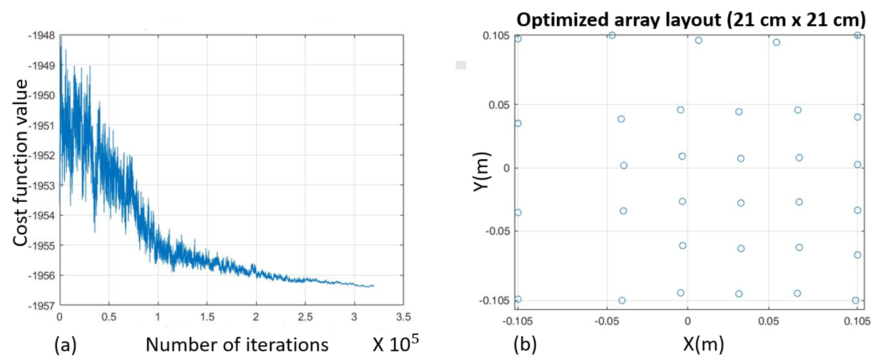
7.2. Thirty-Two-Microphones, [2, 6.4] kHz, Array 21 × 21 cm2

Increasing the number of iterations in the optimization algorithm alone does not fully suppress grating lobes at higher frequencies, even in an optimized field of view. We hypothesize that enlarging the dimensions of the main acoustic lobe provides additional degrees of freedom for the algorithm to minimize secondary grating lobes. A wider main lobe increases the target spatial region for overall sidelobe suppression. However, expanding the filter tap length can sometimes yield unstable and non-convergent solutions. We experimentally evaluate these trade-offs between main lobe width, number of taps (FIR length), and iterations. The following experiments systematically vary lobe parameters and tap length to assess their impact on grating lobe artefacts and algorithm stability. We optimize over an expanded parameter space to determine configurations that maximize grating lobe mitigation while maintaining convergence and solution integrity. This exploration provides practical insights into the interaction between beam pattern specifications, filter design constraints, and robust algorithm convergence for optimal array performance. We report the better results of the following simulation (Figure 15 and Figure 16) in comparison to the previous case:
  • L = 21 cm;
  • of microphones = 32 mic;
  • K = 31 (FIR length);
  • u ∈ [−1.5; 1.5]; v ∈ [−1.41; 1.41];
  • of iterations ≈ 10 5 ;
  • u M a i n L o b e l o w = −0.2; u M a i n L o b e h i g h = 0.2;
  • v M a i n L o b e l o w = −0.2; v M a i n L o b e h i g h = 0.2;
  • Bandwidth = [2000, 6400] Hz.
The 0.21 m array in the bandwidth [2000, 6400] Hz achieves better directivity than the 0.21 m array in the full range [500, 6400] Hz below 4 kHz, confirming substantial miniaturization optimized in a sub-range of frequencies is viable. A sub-range of u and v now optimizes the beampatterns avoiding grating lobes at higher frequencies (Figure 17 and Figure 18), even if this action reduces of course the FOV of Dual Cam 2.0.

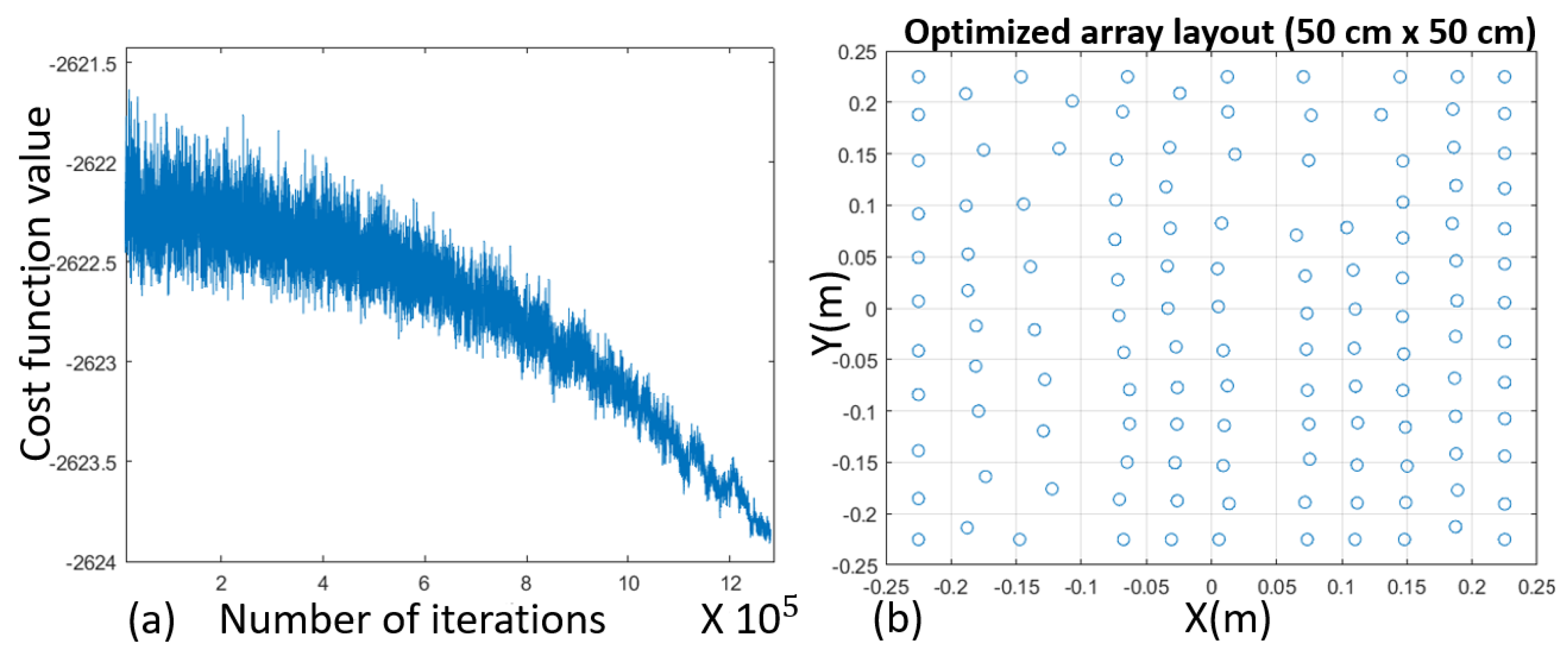
7.3. Thirty-Two-Microphones, [0.5, 6.4] kHz, 21 × 21 cm2 Array

This section compares the performance of the current acoustic device Dual Cam against a new prototype with shortened dimensions but equivalent bandwidth. We simulate this current experimental condition:
  • L = 50 cm;
  • of microphones = 128 mic;
  • K = 7 (FIR length);
  • u ∈ [−1.5; 1.5]; v ∈ [−1.41; 1.41];
  • of iterations ≈ 10 5 ;
  • u M a i n L o b e l o w = −0.06; u M a i n L o b e h i g h = 0.06;
  • v M a i n L o b e l o w = −0.06; v M a i n L o b e h i g h = 0.06;
  • Bandwidth = [500, 6400] Hz.
Simulations are conducted to analyse the key metrics of white noise gain, directivity patterns, and grating lobes. The results demonstrate the feasibility of achieving a compact form factor while maintaining wideband performance through optimization of design parameters.
In our simulation, the third scenario expands the bandwidth to cover Dual Cam 2.0 specifications for comparison with the current device:
  • L = 21 cm;
  • of microphones = 32 mic;
  • K = 31 (FIR length);
  • u ∈ [−1,5; 1.5]; v ∈ [−1,41; 1.41];
  • N° of iterations≈ 10 5 ;
  • u M a i n L o b e l o w = −0.2; u M a i n L o b e h i g h = 0.2;
  • v M a i n L o b e l o w = −0.2; v M a i n L o b e h i g h = 0.2;
  • Bandwidth = [500, 6400] Hz.
Compensating for the larger wavelength at 0.5 kHz required shrinking once again the array to 0.21 × 0.21 m2 to maintain the density with 32 microphones to give the area reduction. The cost convergence in Figure 19a follows a similar trend but more iterations are needed to escape poor local minima. The layout in Figure 19b retains an irregular structure with permutations tailored to the acoustic parameters. The current Dual Cam working prototype (Figure 20) has a better WNG and directivity, especially at low frequencies (Figure 21 and Figure 22); also, the main lobe of the BP and EBPP is sharper (Figure 23 and Figure 24). Instead, the grating lobes at high frequencies are more or less the same. The directivity comparison (Figure 13a) with a 0.21 × 0.21 m2 prototype in the bandwidth [0.5, 6.4] kHz in Figure 21a indicates better sensitivity below 4 kHz. The beam patterns in Figure 14 verify directional selectivity and sidelobe suppression within the band (Figure 21b). Some tradeoffs are highlighted between miniaturization and resolution. Further work is suggested to refine the simulations and investigate the impacts of varying filter lengths (Figure 25). The simulated performance demonstrates that high-fidelity acoustic imaging over audio frequencies can plausibly be achieved with array apertures 4× smaller than the Dual Cam benchmark.
This supports developing compact prototypes based on these optimized configurations. Ongoing research is focused on the physical implementation of miniaturized arrays guided by these modelling results.

8. Hardware Development Considerations

Constructing optimized microphone arrays to realize portable acoustic cameras presents additional implementation challenges including:
  • Fabricating irregular array geometries with a large number of elements;
  • Microphone calibration and mismatch compensation;
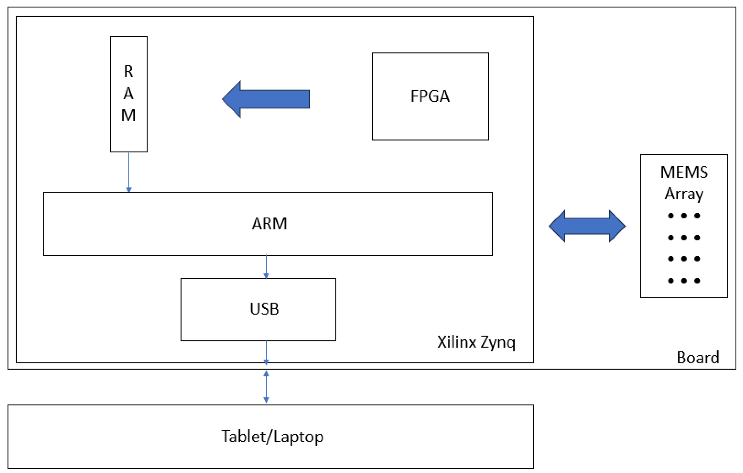
  • Embedded platform with multichannel digitization and processing;
  • Robust beamforming algorithms executable in real time;
  • Packaging, power, and interfacing for field deployment.
The printed circuit board population provides a potential fabrication approach for unconventional layouts. The layout can be rendered as copper traces linking microphone footprints. Micro-electromechanical system (MEMS) technology enables compact sensors [46]. Calibration tools measure each microphone response to derive compensation filters. FPGAs offer parallelism for multichannel acquisition and beamforming [47,48]. Robust and adaptive algorithms help counteract model errors. Energy-efficient architectures would enable battery-powered operation. A USB- or WiFi-linked interface with a smartphone or tablet app could provide deployment flexibility. Ongoing research is focused on addressing these areas to translate the simulated performance gains into practical miniature acoustic cameras for expanded applications. In addition to hardware, robust calibration procedures and beamforming software refinement would help approximate idealized models. User studies assessing video augmented with acoustic imaging for tasks like machine diagnostics can quantify real-world benefits. Developing the signal processing, microphone technologies, and system integration techniques to realize compact acoustic cameras would represent a breakthrough for broader adoption in noise monitoring, condition-based maintenance, virtual reality, and other fields constrained by large form factors today.

9. Conclusions

This paper investigated methodologies to minimize the physical aperture of real-time acoustic cameras for improved mobility.
Acoustic systems rely on an array of microphones to perform directional processing. Reducing the physical aperture of the array typically decreases the angular resolution and introduces grating lobes. However, making the assumption of using higher audio harmonics while maintaining intelligibility without the fundamental frequencies and with careful selection of design parameters, compact arrays may still achieve wideband performance on par with larger arrays. This work investigates this premise through simulation of a current acoustic system and proposed compact prototype. A case study of the Dual Cam prototype that utilizes a 0.5 × 0.5 m2, 128−microphone planar array to generate acoustic field visualizations in real time revealed limitations around size, weight, power, and computational complexity that restrict widespread adoption. To transform such cameras into portable devices, we proposed co-optimizing the array layout and beamforming filters through simulations to concentrate directional sensitivity and minimize artefacts. Analyses quantified that a 32−element 0.21 × 0.21 m2 array optimized for the bandwidth [2, 6.4] kHz operation could theoretically achieve better directivity than the full-scale Dual Cam prototype up to 4 kHz, confirming substantial miniaturization is viable with tolerable performance trade-offs. Ongoing efforts are focused on constructing miniature microphone arrays guided by these numerical optimizations to develop hand-held acoustic cameras that interface with tablets and smartphones for easy deployment. Realizing compact, real-time acoustic imaging devices could expand applications in structural health monitoring, urban noise mapping, VR/AR audio rendering, and other fields currently constrained by large form factors. This paper provided an array of signal processing insights to guide physical prototype development towards transforming acoustic imaging capabilities from constrained lab settings into widely accessible mobile platforms. With further progress in microphone technologies, embedded computing, and calibration techniques, ubiquitous acoustic imaging could become viable—providing uniquely valuable spatial and semantic context across applications ranging from the industrial internet of things to smart city sound monitoring (Figure 26).

Funding

This research received no external funding.

Data Availability Statement

Not applicable.

Conflicts of Interest

The author declares no conflict of interest.

References

  1. Dmochowski, J.P.; Benesty, J. Steered Beamforming Approaches for Acoustic Source Localization. In Speech Processing in Modern Communication; Cohen, I., Benesty, J., Gannot, S., Eds.; Springer Topics in Signal Processing; Springer: Berlin/Heidelberg, Germany, 2010; Volume 3. [Google Scholar] [CrossRef]
  2. Rafaely, B. Fundamentals of Spherical Array Processing; Springer: Berlin/Heidelberg, Germany, 2019. [Google Scholar]
  3. Van Veen, B.D.; Buckley, K.M. Beamforming: A versatile approach to spatial filtering. IEEE Assp Mag. 1988, 5, 4–24. [Google Scholar] [CrossRef] [PubMed]
  4. Jombo, G.; Zhang, Y. Acoustic-Based Machine Condition Monitoring—Methods and Challenges. Eng 2023, 4, 47–79. [Google Scholar] [CrossRef]
  5. Na, Y. An Acoustic Traffic Monitoring System: Design and Implementation. In Proceedings of the 2015 IEEE 12th International Conference on Ubiquitous Intelligence and Computing and 2015 IEEE 12th International Conference on Autonomic and Trusted Computing and 2015 IEEE 15th International Conference on Scalable Computing and Communications and Its Associated Workshops (UIC-ATC-ScalCom), Beijing, China, 10–14 August 2015. [Google Scholar] [CrossRef]
  6. António, R. On acoustic gunshot localization systems. In Proceedings of the Society for Design and Process Science SDPS-2015, Fort Worth, TX, USA, 1–5 November 2015; pp. 558–565. [Google Scholar]
  7. Lluís, F.; Martínez-Nuevo, P.; Møller, M.B.; Shepstone, S.E. Sound field reconstruction in rooms: Inpainting meets super-resolution. J. Acoust. Soc. Am. 2020, 148, 649–659. [Google Scholar] [CrossRef] [PubMed]
  8. Yan, J.; Zhang, T.; Broughton-Venner, J.; Huang, P.; Tang, M.-X. Super-Resolution Ultrasound Through Sparsity-Based Deconvolution and Multi-Feature Tracking. IEEE Trans. Med. Imaging 2022, 41, 1938–1947. [Google Scholar] [CrossRef]
  9. Crocco, M.; Cristani, M.; Trucco, A.; Murino, V. Audio Surveillance: A Systematic Review. ACM Comput. Surv. 2016, 48, 46. [Google Scholar] [CrossRef]
  10. Crocco, M.; Martelli, S.; Trucco, A.; Zunino, A.; Murino, V. Audio Tracking in Noisy Environments by Acoustic Map and Spectral Signature. IEEE Trans. Cybern. 2018, 48, 1619–1632. [Google Scholar] [CrossRef]
  11. Worley, R.; Dewoolkar, M.; Xia, T.; Farrell, R.; Orfeo, D.; Burns, D.; Huston, D. Acoustic Emission Sensing for Crack Monitoring in Prefabricated and Prestressed Reinforced Concrete Bridge Girders. J. Bridge Eng. 2019, 24, 04019018. [Google Scholar] [CrossRef]
  12. Bello, J.P.; Silva, C.; Nov, O.; Dubois, R.L.; Arora, A.; Salamon, J.; Mydlarz, C.; Doraiswamy, H. SONYC: A system for monitoring, analyzing, and mitigating urban noise pollution. Commun. ACM 2019, 62, 68–77. [Google Scholar] [CrossRef]
  13. Sun, X. Immersive audio, capture, transport, and rendering: A review. Apsipa Trans. Signal Inf. Process. 2021, 10, e13. [Google Scholar] [CrossRef]
  14. Zhang, H.; Wang, J.; Li, Z.; Li, J. Design and Implementation of Two Immersive Audio and Video Communication Systems Based on Virtual Reality. Electronics 2023, 12, 1134. [Google Scholar] [CrossRef]
  15. Padois, T.; St-Jacques, J.; Rouard, K.; Quaegebeur, N.; Grondin, F.; Berry, A.; Nélisse, H.; Sgard, F.; Doutres, O. Acoustic imaging with spherical microphone array and Kriging. JASA Express Lett. 2023, 3, 042801. [Google Scholar] [CrossRef]
  16. Chu, Z.; Yin, S.; Yang, Y.; Li, P. Filter-and-sum based high-resolution CLEAN-SC with spherical microphone arrays. Appl. Acoust. 2021, 182, 108278. [Google Scholar] [CrossRef]
  17. Ward, D.B.; Kennedy, R.A.; Williamson, R.C.; Brandstein, M. Microphone Arrays Signal Processing Techniques and Applications (Digital Signal Processing); Springer: Berlin/Heidelberg, Germany, 2001. [Google Scholar]
  18. Crocco, M.; Trucco, A. Design of Superdirective Planar Arrays With Sparse Aperiodic Layouts for Processing Broadband Signals via 3-D Beamforming. IEEE/ACM Trans. Audio Speech Lang. Process. 2014, 22, 800–815. [Google Scholar] [CrossRef]
  19. Crocco, M.; Trucco, A. Stochastic and Analytic Optimization of Sparse Aperiodic Arrays and Broadband Beamformers WITH Robust Superdirective Patterns. IEEE Trans. Audio Speech Lang. Process. 2012, 20, 2433–2447. [Google Scholar] [CrossRef]
  20. Mars, R.; Reju, V.G.; Khong, A.W.H.; Hioka, Y.; Niwa, K. Chapter 12—Beamforming Techniques Using Microphone Arrays; Chellappa, R., Theodoridis, S., Eds.; Academic Press Library in Signal Processing; Academic Press: Cambridge, MA, USA, 2018; Volume 7, pp. 585–612. ISBN 9780128118870. [Google Scholar] [CrossRef]
  21. Hansen, R.C. Phased Array Antennas, 2nd ed.; John Wiley & Sons, Inc.: Hoboken, NJ, USA, 2009; ISBN 978-0-470-40102-6. [Google Scholar]
  22. Cox, H.; Zeskind, R.; Kooij, T. Practical supergain. IEEE Trans. Acoust. Speech, Signal Process. 1986, 34, 393–398. [Google Scholar] [CrossRef]
  23. Kates, J.M. Superdirective arrays for hearing aids. J. Acoust. Soc. Am. 1993, 94, 1930–1933. [Google Scholar] [CrossRef] [PubMed]
  24. Bitzer, J.; Simmer, K.U. Superdirective microphone arrays. In Microphone Arrays: Signal Processing Techniques and Applications; Brandstein, M.S., Ward, D.B., Eds.; Springer: New York, NY, USA, 2001; pp. 19–38. [Google Scholar]
  25. Van Trees, H.L. Optimum Array Processing: Part IV of Detection, Estimation, and Modulation Theory; John Wiley & Sons, Inc.: Hoboken, NJ, USA, 2002. [Google Scholar]
  26. Ward, D.B.; Kennedy, R.A.; Williamson, R.C. Theory and design of broadband sensor arrays with frequency invariant far-field beam patterns. J. Acoust. Soc. Am. 1995, 97, 1023–1034. [Google Scholar] [CrossRef]
  27. Crocco, M.; Trucco, A. Design of Robust Superdirective Arrays With a Tunable Tradeoff Between Directivity and Frequency-Invariance. IEEE Trans. Signal Process. 2011, 59, 2169–2181. [Google Scholar] [CrossRef]
  28. Doclo, S. Multi-microphone noise reduction and dereverberation techniques for speech applications. Ph.D. Thesis, Katholieke Universiteit Leuven, Leuven, Belgium, 2003. Available online: ftp://ftp.esat.kuleuven.ac.be/stadius/doclo/phd/ (accessed on 14 June 2023).
  29. Crocco, M.; Trucco, A. The synthesis of robust broadband beamformers for equally-spaced linear arrays. J. Acoust. Soc. Am. 2010, 128, 691–701. [Google Scholar] [CrossRef]
  30. Mabande, E. Robust Time-Invariant Broadband Beamforming as a Convex Optimization Problem. Ph.D. Thesis, Friedrich-Alexander-Universität, Erlangen, Germany, 2015. Available online: https://opus4.kobv.de/opus4-fau/frontdoor/index/index/year/2015/docId/6138/ (accessed on 14 June 2023).
  31. Trucco, A.; Traverso, F.; Crocco, M. Robust superdirective end-fire arrays. In Proceedings of the 2013 MTS/IEEE OCEANS—Bergen, Bergen, Norway, 10–13 June 2013; pp. 1–6. [Google Scholar] [CrossRef]
  32. Traverso, F.; Crocco, M.; Trucco, A. Design of frequency-invariant robust beam patterns by the oversteering of end-fire arrays. Signal Process. 2014, 99, 129–135. [Google Scholar] [CrossRef]
  33. Trucco, A.; Crocco, M. Design of an Optimum Superdirective Beamformer Through Generalized Directivity Maximization. IEEE Trans. Signal Process. 2014, 62, 6118–6129. [Google Scholar] [CrossRef]
  34. Trucco, A.; Traverso, F.; Crocco, M. Broadband performance of superdirective delay-and-sum beamformers steered to end-fire. J. Acoust. Soc. Am. 2014, 135, EL331–EL337. [Google Scholar] [CrossRef] [PubMed]
  35. Doclo, S.; Moonen, M. Superdirective Beamforming Robust Against Microphone Mismatch. IEEE Trans. Audio, Speech, Lang. Process. 2007, 15, 617–631. [Google Scholar] [CrossRef]
  36. Crocco, M.; Trucco, A. A Synthesis Method for Robust Frequency-Invariant Very Large Bandwidth Beamforming. In Proceedings of the 18th European Signal Processing Conference (EUSIPCO 2010), Aalborg, Denmark, 23–27 August 2010; pp. 2096–2100. [Google Scholar]
  37. Trucco, A.; Crocco, M.; Traverso, F. Avoiding the imposition of a desired beam pattern in superdirective frequency-invariant beamformers. In Proceedings of the 26th Annual Review of Progress in Applied Computational Electromagnetics, Tampere, Finland, 26–29 April 2010; pp. 952–957. [Google Scholar]
  38. Doclo, S.; Moonen, M. Design of broadband beamformers robust against gain and phase errors in the microphone array characteristics. IEEE Trans. Signal Process. 2003, 51, 2511–2526. [Google Scholar] [CrossRef]
  39. Mabande, E.; Schad, A.; Kellermann, W. Design of robust superdirective beamformers as a convex optimization problem. In Proceedings of the 2009 IEEE International Conference on Acoustics, Speech and Signal Processing, Taipei, Taiwan, 19–24 April 2009; pp. 77–80. [Google Scholar] [CrossRef]
  40. Greco, D.; Trucco, A. Superdirective Robust Algorithms’ Comparison for Linear Arrays. Acoustics 2020, 2, 707–718. [Google Scholar] [CrossRef]
  41. Pérez, A.F.; Sanguineti, V.; Morerio, P.; Murino, V. Audio-Visual Model Distillation Using Acoustic Images. In Proceedings of the 2020 IEEE Winter Conference on Applications of Computer Vision (WACV), Snowmass, CO, USA, 1–5 March 2020; pp. 2843–2852. [Google Scholar] [CrossRef]
  42. Sanguineti, V.; Morerio, P.; Pozzetti, N.; Greco, D.; Cristani, M.; Murino, V. Leveraging acoustic images for effective self-supervised audio representation learning. In Proceedings of the Computer Vision—ECCV 2020: 16th European Conference, Glasgow, UK, 23–28 August 2020; Part XXII 16. pp. 119–135. [Google Scholar]
  43. Ward, D.B.; Kennedy, R.A.; Williamson, R.C. FIR filter design for frequency invariant beamformers. IEEE Signal Process. Lett. 1996, 3, 69–71. [Google Scholar] [CrossRef]
  44. Sanguineti, V.; Morerio, P.; Bue, A.D.; Murino, V. Unsupervised Synthetic Acoustic Image Generation for Audio-Visual Scene Understanding. IEEE Trans. Image Process. 2022, 31, 7102–7115. [Google Scholar] [CrossRef]
  45. Kirkpatrick, S.; Gelatt, C.D., Jr.; Vecchi, M.P. Optimization by Simulated Annealing. Science 1983, 220, 671–680. [Google Scholar] [CrossRef]
  46. Chae, M.S.; Yang, Z.; Yuce, M.R.; Hoang, L.; Liu, W. A 128-channel 6 mW wireless neural recording IC with spike feature extraction and UWB transmitter. IEEE Trans. Neural Syst. Rehabil. Eng. 2009, 17, 312–321. [Google Scholar] [CrossRef]
  47. Paolo, M.; Alessandro, C.; Gianfranco, D.; Michele, B.; Francesco, C.; Davide, R.; Luigi, R.; Luca, B. Neuraghe: Exploiting CPU-FPGA synergies for efficient and flexible CNN inference acceleration on zynQ SoCs. ACM Trans. Reconfigurable Technol. Syst. 2017, 11, 1–24. [Google Scholar] [CrossRef]
  48. Da Silva, B.; Braeken, A.; Touhafi, A. FPGA-Based Architectures for Acoustic Beamforming with Microphone Arrays: Trends, Challenges and Research Opportunities. Computers 2018, 7, 41. [Google Scholar] [CrossRef]
Figure 1. Dual Cam prototype integrates co-located acoustic and visual imaging modalities using a planar microphone array paired with a video camera [10].
Applsci 13 11110 g001
Figure 2. Broadband beamforming issues (1-D): (a) low directivity at low frequencies and (b) aliasing at high frequencies. B ( f , ϕ ) , beampattern; f, function of frequency; ϕ , DOA (direction of arrival) [17].
Applsci 13 11110 g002
Figure 3. Simulation of a periodic 32−microphone positioning on a planar array 25 × 25 cm2.
Applsci 13 11110 g003
Figure 4. Two−dimensional beam pattern using a periodic positioning of 32−microphones on a planar array 25 × 25 cm2 (Figure 3) at different frequencies: (a) beam pattern at 2 kHz, (b) beam pattern at ≈6 kHz, both functions of θ and ϕ (u and v; see later on). Increasing the frequency, the grating lobes equal the main central lobe. The colorbar maps from 0 dB (yellow) to -30 dB (blue).
Applsci 13 11110 g004
Figure 5. From raw audio (a) to 3-D acoustic image (b) to 2-D energy heatmap (c) (from red maximum sound to blue minimum sound) [44].
Applsci 13 11110 g005
Figure 6. Three examples from a collected dataset. We visualize the acoustic image by summing the energy of all frequencies for each acoustic pixel. The resulting map (from red maximum sound to blue minimum sound) is overlaid on the corresponding RGB frame. From left to right: (a) drone, (b) train, (c) vacuum cleaner [42].
Applsci 13 11110 g006
Figure 7. New Dual Cam 2.0 POC (proof of concept) idea. The periodic positioning of the microphones is generic and for illustrative purposes only.
Applsci 13 11110 g007
Figure 8. The Dual Cam board is based on an FPGA that reads continuously from the I2S MEMS microphones (TDK/InvenSense); using a programmed DMA the read microphones values are stored in a RAM buffer. In our new proof of concept (POC) the processor can easily read data from RAM and redirect them to the USB port.
Applsci 13 11110 g008
Figure 9. Conceptual framework in the microphone array simulation.
Applsci 13 11110 g009
Figure 10. Cartesian coordinates system and steering angles ( θ 0 , ϕ 0 ).
Applsci 13 11110 g010
Figure 11. Flow chart of Simulated Annealing algorithm for function cost minimization.
Applsci 13 11110 g011
Figure 12. Simulation results for [2, 6.4] kHz optimization of a 32−elements 0.25 m acoustic array: (a) cost function convergence over 100 iterations, (b) optimized 32−microphone 0.25 m array layout.
Applsci 13 11110 g012
Figure 13. (a) Directivity and (b) white noise gain metrics confirm reasonable performance across the [2, 6.4] kHz band from the 0.25 m array.
Applsci 13 11110 g013
Figure 14. Simulation array 25 × 25 cm2. Beam patterns within the optimization band and the aperiodic microphone localization exhibit low sidelobes and main lobe focusing (Figure 4). (a) 2 kHz, (b) ≈4 kHz, (c) ≈6 kHz.
Applsci 13 11110 g014
Figure 15. Simulation results for [2, 6.4] kHz optimization of a 32−element 0.21 m acoustic array: (a) cost function convergence over 10 5 iterations, (b) optimized 32−microphone 0.21 m array layout.
Applsci 13 11110 g015
Figure 16. (a) Directivity and (b) white noise gain metrics confirm reasonable performance across the [2,6.4] kHz band even from the reduced 0.21 m array.
Applsci 13 11110 g016
Figure 17. Simulation results for [2, 6.4] kHz optimization of a 32−element 0.21 m acoustic array. Beampatten comparison: BP (left) vs EBPP (right) at 2 kHz.
Applsci 13 11110 g017
Figure 18. Simulation results for [2, 6.4] kHz optimization of a 32−element 0.21 m acoustic array. Beampatten comparison: BP (left) vs EBPP (right) at ≈6 kHz.
Applsci 13 11110 g018
Figure 19. Simulation results for [0.5, 6.4] kHz optimization of a 32−element 0.21 × 0.21 m2 planar acoustic array: (a) cost function convergence over 10 5 iterations, (b) optimized 32−microphone 0.21 m array layout.
Applsci 13 11110 g019
Figure 20. Current Dual Cam prototype. Simulation results for [0.5, 6.4] kHz optimization of a 128−element 0.50 × 0.50 m2 planar acoustic array: (a) cost function convergence over ≈ 10 5 iterations, (b) optimized 128−microphone 0.50 m array layout.
Applsci 13 11110 g020
Figure 21. Dual Cam 2.0 with larger audio bandwidth [500, 6400] Hz on a 0.21 × 0.21 m2 array. Directivity (a) and WNG (b).
Applsci 13 11110 g021
Figure 22. Current Dual Cam prototype. Expected beam pattern power at different frequencies: (a) 500 Hz, (b) ≈2.5 kHz, (c) ≈6 kHz.
Applsci 13 11110 g022
Figure 23. Current Dual Cam prototype: (a) Directivity and (b) WNG over the full bandwidth [500, 6400] Hz on a 50 × 50 cm2 array.
Applsci 13 11110 g023
Figure 24. Dual Cam 2.0 cted beam pattern power at different frequencies: (a) 500 Hz, (b) ≈2.5 kHz, (c) ≈6 kHz.
Applsci 13 11110 g024
Figure 25. Dual Cam 2.0 with larger audio bandwidth [0.5, 6.4] kHz: effect of the FIR length on the metrics of the evaluation. (a) Directivity with K = 7 (red) vs K = 21 (blue); (b) WNG with K = 7 (red) vs. K = 21 (blue).
Applsci 13 11110 g025
Figure 26. Dual Cam 2.0 Business Model Canvas.
Applsci 13 11110 g026
Disclaimer/Publisher’s Note: The statements, opinions and data contained in all publications are solely those of the individual author(s) and contributor(s) and not of MDPI and/or the editor(s). MDPI and/or the editor(s) disclaim responsibility for any injury to people or property resulting from any ideas, methods, instructions or products referred to in the content.

