Abstract
A personal audio system has a wide application prospect in people’s lives, which can be implemented by sound field control technology. However, the current sound field control technology is mainly based on sound pressure or its improvement, ignoring another physical property of sound: particle velocity, which is not conducive to the stability of the entire reconstruction system. To address the problem, a sound field method is constructed in this paper, which minimizes the reconstruction error in the bright zone, minimizes the loudspeaker array effort in the reconstruction system, and at the same time controls the particle velocity and sound pressure of the dark zone. Five unevenly placed loudspeakers were used as the initial setup for the computer simulation experiment. Simulation results suggest that the proposed method is better than the PM (pressure matching) and EDPM (eigen decomposition pseudoinverse method) methods in the bright zone in an acoustic contrast index, the ACC (acoustic contrast control) method in a reconstruction error index, and the ACC, PM, and EDPM methods in the bright zone in a loudspeaker array effort index. The average array effort of the proposed method is the smallest, which is about 9.4790, 8.0712, and 4.8176 dB less than that of the ACC method, the PM method in the bright zone, and the EDPM method in the bright zone, respectively, so the proposed method can produce the most stable reconstruction system when the loudspeaker system is not evenly placed. The results of computer experiments demonstrate the performance of the proposed method, and suggest that compared with traditional methods, the proposed method can achieve more balanced results in the three indexes of acoustic contrast, reconstruction error, and loudspeaker array effort on the whole.
1. Introduction
Based on multizone sound field reconstruction technologies, a personal audio system can be used to concentrate sound effects in a listening area without affecting listeners in other areas. A bright zone and a dark zone can be generated by multizone sound field reconstruction techniques. The desired sound pressure field could be generated in the bright zone, while the sound pressure level is attenuated in the dark zone. Personal audio systems can be used in game systems, audio system exhibits, home theaters, car audio systems, etc. [1]. With the development of sound field reconstruction technology, more and more people pay attention to personal audio systems. Many researchers have put forward many new research methods and techniques for a personal audio system.
The acoustic contrast control (ACC) method was introduced by Choi et al., which solves loudspeakers’ allocation coefficients by maximizing the acoustic contrast between the bright zone and the dark zone [2]. However, the ACC method does not control the phase, and its energy is unevenly distributed in the bright zone, which will affect the subjective listening experience of listeners. The pressure matching (PM) method can solve these problems by minimizing the error between the desired sound pressure and the reconstructed sound pressure at control points [3]. Additionally, the planarity control (PC) method was proposed [4], which filters the sound pressure at the control points spatially, and maximizes the energy of the bright zone under the constraint of the dark zone energy based on the super-directional beamforming. The advantage of the PM method and the PC method is that they can generate a directional sound field in the range of the bright zone, while the disadvantage of the PM method and the PC method is that the acoustic contrasts generated by them are smaller than that of the ACC method. Shin et al. introduced a method that maximizes the acoustic energy difference, which changes the focus of the ACC method by focusing on the ratio of the mean square sound pressure difference between the bright and dark zones. The comparison experiments with the ACC method show that this method can maintain the sound pressure difference between two listening zones and improve the radiation efficiency of sound space. In addition, this method is simple to calculate [5]. Chang et al. tried to take advantage of the ACC method and the PM method and proposed the ACC–PM method by combining these two methods. By selecting the appropriate adjustment factor, the ACC–PM method can obtain the tradeoff effect between the bright zone reconstruction error and acoustic contrast [6]. Based on the PM approach, Olivieri et al. proposed a beamforming approach to control the tradeoff between listener position sound field quality and directivity performance. This proposed method selects control points that contribute to the PM cost function in a frequency-dependent manner according to the angular distance between control points relative to a given wavelength [7]. Based on the PM method, Afghah et al. proposed the eigen decomposition pseudoinverse method (EDPM) [8]. This method constructs a regularization strategy to solve the pseudoinverse of ill-conditioned matrices, replacing the Tikhonov regularization method traditionally used in the PM method. This method is used to improve the performance at dark points without generating artifacts at bright points. In view of the robustness and regularization of the ACC method, Elliott et al. proposed that robustness could be enhanced by imposing limits on array effort. Robustness can generally be improved by a regularization method, but good regularization parameters are often difficult to choose [9]. Zhu et al. proposed a robust sound zone reconstruction design framework that solves the parameters by acoustic modeling. However, they did not examine the relationship between different loudspeaker directivities and robust optimization and explore the accuracy required for robust ACC acoustic modeling [10]. Han et al. proposed a method for acoustic contrast control in a wave domain for three dimension cases. The three-dimensional sound field is represented by spherical harmonic decomposition, and the sound energy of the interested region is calculated. The three-dimensional multizone sound field is reconstructed by using a planar circular loudspeaker array instead of a spherical one. Experiments show that this method is better than the ACC method in high-frequency acoustic contrast performance [11]. The time-domain ACC method (TACC) is favored because it can optimize the entire bandwidth by one step, but the disadvantage of TACC is that the frequency response is not uneven. In order to explain this problem theoretically, Hu et al. constructed a progressively equivalent form of TACC in frequency domain, and demonstrated that TACC has an inclination to fetch frequency constituents of the largest contrast [12]. By considering the signal feature and human auditory system, Lee et al. introduced a sound zone control frame called perception VAST. The experiments suggest that the perception VAST method performs better than the ACC and PM methods in terms of the perceptive index of STOI and PESQ [13]. Then, in order to make the leakage error under a fixed acoustic contrast as imperceptible as possible, they extended this work to an adaptive case and proposed a time-domain sound region control method using a variable span tradeoff filter [14]. To reduce computational complexity, they then proposed two VAST framework-based approaches (narrowband approach and broadband approach) in the discrete Fourier transform domain [15]. Ryu et al. proposed a personal audio effect controller whose effects change linearly with the customer’s input. The weight trajectories of loudspeakers are modeled as continuous functions based on piecewise linear approximations of the performance variation. The experimental results show that the controller can regulate the system performance linearly [16]. Hu et al. introduced a sound field control method in a time domain based on sound pressure and particle velocity for single-zone sound field reconstruction. In this method, the eigenvalue-decomposition-based way and the conjugate-gradient way are used to decrease the complexity of computing [17]. In order to reduce the requirements on microphone placement geometry and a control sound field in the whole region, Du et al. proposed a two-region 2D sound field reproduction approach based on equivalent source and the ACC method. The goal of this method is to maximize the acoustic energy difference between the two regions [18]. Additionally, Du et al. introduced another two-region sound field reconstruction method based on equivalent source and the PM and ACC methods. Compared with the traditional method, sound field control in a dark region by Du’s method is not limited to several points at the boundary of the dark zone, but extends to the whole dark zone [19]. The number and location of loudspeakers have important influence on the reconstruction effect in multizone sound field reconstruction. When people perform multizone sound field reconstruction, people often arrange the loudspeakers in a circular, linear, and curved fashion, but these arrangements are obtained by experience. To solve the problem, Zhu et al. introduced a method to select the required number of loudspeaker locations from candidate loudspeaker locations iteratively [20]. Then, enlightened by the theory in [21], Zhao et al. proposed an evolutionary optimization approach based on a candidate location set to optimize loudspeaker array placement [22]. Different from the iterative method, this method eliminates one loudspeaker from the loudspeaker candidate set at each iteration. Zhong et al. investigated the feasibility of using multiparameter array loudspeakers to remotely generate a quiet zone in a free sound field. They obtained the relationship between the size of the quiet zone and the number of secondary sound sources and the wavelength of secondary sound sources in two and three dimension cases [23]. Abe et al. proposed an amplitude matching algorithm for multizone sound field control, which produces the expected amplitude distribution in the designated region by alternating the direction method of multipliers, without paying attention to phase distribution [24].
There are also some experts who have studied the application of personal audio systems. Elliott et al. studied the application of the ACC method to a headrest [25]. Cheer et al. conducted some research on the application of personal audio systems to mobile phones [26]. Cheer et al. also put personal audio systems into a car with two loudspeaker arrays [27]. Different from the method described in the literature [27], Liao et al. proposed to fix loudspeaker arrays on the ceiling of a car compartment in order to produce separate high-frequency listening regions in the front and rear seats of the car compartment [28]. They also investigated the geometric size design method for ceiling-mounted loudspeaker arrays and target sound pressures’ selection method. Compared with the system in the literature [27], the system proposed by Liao et al. shows obvious performance improvement in the frequency range of 1–4 kHz. Based on an line loudspeaker array mounted on a flat-screen TV in the form of a bar loudspeaker, Choi proposed two kinds of sound field control systems for home applications that are real-time. One kind of system is a personal audio system that makes users at different positions experience independent sound effects by reducing the mutual interference of different sound zones; another kind of system can exert an influence on the spatial audio scene [29].
The sound property considered by most existing sound field control technologies is sound pressure. Additionally, many of the sound field control technologies proposed by researchers are improved techniques based on sound pressure. Sound pressure and particle velocity can be used to describe sound [30]. Additionally, it is pointed out in [31] that when loudspeakers are not evenly placed, the loudspeaker signal obtained by controlling the sound pressure of a single region is less stable than the loudspeaker signal obtained by controlling the particle velocity of a single region. Because in real life, many loudspeaker arrays are not evenly placed, particle velocity should be considered in addition to sound pressure in the design of sound field control methods. On the basis of traditional methods, a sound field control method based on sound pressure and particle velocity is introduced in order to reconstruct a sound field in the bright zone better, reduce acoustic energy in the dark zone, and pay attention to the stability of the system.
The main contributions of this paper are as follows: based on the traditional sound field control technology, a new sound field control method is proposed by introducing particle velocity. The proposed method attempts to minimize the reconstruction error in the bright zone and minimize the loudspeaker array effort while controlling the sound pressure and particle velocity in the dark zone. The proposed method attempts to control or optimize acoustic contrast, reconstruction error, and array effort at the same time. The model of the proposed method contains three weight factors; this paper introduces their functions and gives their selection methods. The content of this paper is arranged as follows: Section 1 mainly describes the development status of sound field control technology. Section 2 describes three existing sound field control technologies and analyzes their advantages and disadvantages. Section 3 introduces the model of this new method and parameter selection method of the model. Section 4 introduces the comparison experiment between traditional methods and the proposed method, and analyzes and discusses the results. Section 5 gives the conclusions.
2. Three Traditional Sound Field Control Methods
This part introduces three traditional acoustic field reconstruction methods: ACC [2], PM [3], and EDPM [8]. The ACC and PM methods in the bright zone are relatively important methods and have important influence in the field of sound field control. Acoustic contrast and reconstruction error are important indicators to measure the effect of sound field control. The ACC method is used to maximize acoustic contrast, so it has the maximum acoustic contrast. The PM method in the bright zone works to minimize the reconstruction error in the bright zone, so it has minimal reconstruction error. The ACC method and the PM method in the bright zone are the best methods in a certain index, and compared with them, the advantages and disadvantages of the proposed methods can be better displayed. The EDPM method in the bright zone is an improvement of the PM method in the bright zone, and they are essentially the same class of methods that try to minimize the reconstruction error in the bright zone. The EDPM method in the bright zone is relatively new compared with the PM method in the bright zone, so it is necessary to compare the proposed method with the EDPM method in the bright zone.
2.1. ACC Method [2]
The ratio of the sound potential energy density of the bright region to the sound potential energy density of the dark region is the definition of acoustic contrast. The goal of the ACC method is to make the acoustic contrast to obtain the maximum value. The formula for calculating acoustic contrast is
where the bright zone is labeled , and the dark zone is labeled . The bright zone volume is labeled , and the dark zone volume is labeled . is the sound pressure in the bright zone, and is the sound pressure in the dark zone as shown in Figure 1.
is source strengths, which is the vector. is the sound pressure transfer function vector in the bright zone, which is a dimension, and is the sound pressure transfer function vector in the dark zone, which also is a dimension. M is the number of sources or loudspeakers. Spatial correlation matrices in the bright zone and the dark zone are labeled and , respectively.
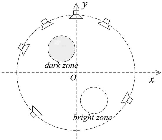
Figure 1.
Loudspeaker array and sound zone diagram.
The acoustic contrast reaches its maximum value when the eigenvector associated with the maximum eigenvalue of is equal to the source strengths. The source strengths at this point are the optimal source strengths.
2.2. PM Method [3]
As shown in Figure 1, it is assumed that M loudspeakers (they also indicate the location of loudspeakers) are placed on the same ring, with s sampling points (they also indicate the location of sampling points) in the bright zone and t sampling points in the dark zone. We suppose that the sound pressure produced by the original source in the bright and the dark zone, respectively, are
where is the amplitude modulation factor. Suppose that the sound pressure generated by M loudspeakers at point () in the bright zone and at point () in the dark zone are, respectively,
The sound pressure transfer function is labeled [32] or , where
If we want to recover the sound pressure produced by the original source in the bright zone, the equation constructed by the PM method is
Formula (10) can also be expressed as
The solution of Equation (11) is ; the inverse of a matrix is labeled . We call this method the PM method in the bright zone.
If we want to recover the pressure generated by the original sound source in both the bright and dark zones, the equation constructed by the PM method is
Formula (12) can also be written as
The solution of Formula (12) can be obtained by .
2.3. EDPM Method [8]
The EDPM method is described in detail in [8]. Here, we mainly introduce the EDPM method in the bright zone, which is similar to the EDPM method. The eigen decomposition theory tells us that a square matrix can be decomposed as follows:
where is a matrix of columnwise eigenvectors, is a diagonal matrix of eigenvalues, and its main diagonal elements are eigenvalues When Tikhonov regularization is applied to the matrix , we can obtain
Inspired by Tikhonov regularization, the pseudoinverse of can be replaced as follows:
where is a scalar and moderator; it goes from 0 to infinity. The main diagonal elements of are
The solution of Formula (11) can be obtained by Tikhonov regularization:
where the Hermitian transpose is labeled H, the identity matrix is labeled I, and the regularization factor is labeled .
2.4. Comparison of Three Traditional Methods
The ACC method can obtain the maximum acoustic contrast, but it does not take into account the sound field reproduction error in the bright region. The PM method in the bright zone can reduce the sound field reproduction error in the bright zone, but it does not pay attention to the acoustic contrast about the bright zone and the dark zone. In the PM method, increasing array efforts by Tikhonov regularization does not minimize well the reconstruction error at dark points. However, the EDPM method can improve dark points’ performance close to that of an elimination method. The EDPM method in the bright zone also does not focus on the acoustic contrast about the bright zone and the dark zone.
3. Proposed Method
This section describes a sound field control optimization model.
3.1. Sound Field Control Method Optimization Model
Reference [30] points out that sound can be described by sound pressure and particle velocity. Reference [31] points out that when loudspeakers are placed unevenly, the loudspeaker signal obtained by controlling the sound pressure of a single region is less stable than the loudspeaker signal obtained by controlling the particle velocity of a single region. Inspired by these conclusions and combined with traditional sound field control methods, this paper proposes a sound field control method that minimizes the error of sound field reproduction in the bright zone, minimizes array effort, and controls the sound pressure and particle velocity in the dark zone at the same time. It is expected to improve the sound field reproduction effect in the bright zone, improve the stability of a loudspeaker array system, and reduce the acoustic energy radiation in the dark zone. The proposed method can be formulated as a constrained optimization problem as follows:
where and are weight factors and , , indicates the threshold and is greater than zero, stands for the power of sound pressure error between the original sound field pressure and the reproduced sound field pressure in the bright zone, stands for dark zone sound energy, stands for sound source power or control effort, and stands for the radial particle velocity of the dark zone:
where r is the distance between point and and , k is the wave number, , is the particle velocity transmission function between a loudspeaker at and point [31], stands for the radial particle velocity transmission function, and is the unit radial vector perpendicular to the surface of the dark zone and is inward.
The cost function of the proposed method includes the error of reconstructed sound pressure in the bright zone, acoustic energy in the dark zone, and sound source power. The three weight factors , , and have their own functions in the model. is used to modulate the sound pressure error in the bright zone and acoustic energy in the dark zone, is used to adjust sound source power, and is used to control the value of particle velocity in the dark zone. The selection strategy of the parameters , , and is described in the next part. The optimization problem in Equation (20) can be solved using the convex optimization software CVX [33,34,35].
3.2. The Selection of Parameters and
Assume that the initial setup of a loudspeaker system is consistent with the experimental section below. Suppose that the value of ranges from 0.1 to 0.9; the change step is 0.1; the value of are 0.1, 0.4, 0.6, and 0.9, respectively; and the original sound source signals are 200, 500, 800, and 1000 Hz, respectively. With different values of , the relationship between the cost function and the parameter is shown in Figure 2, Figure 3, Figure 4 and Figure 5, respectively. These graphs show that the value of the relevant cost function increases with the gradual increase in the value of on the whole. For all values of , the cost function ranges from approximately 0.01 to 0.1. The smaller the value of , the stronger the control on the acoustic energy minimization in the dark zone, and the weaker the control on the sound pressure error minimization in the bright zone. The principle for selecting the value of the parameter is that the smaller the cost function is, the better the system performs. However, the cost function changes little from 0.01 to 0.1. In the meantime, the sound pressure error in the bright zone has great influence on the auditory sensation. Taking these factors into consideration, the value of is chosen to be 0.9. We can see from these figures that, with the constant increase in the parameter , when reaches a certain value, the value of the corresponding cost function basically remains unchanged for a selected value of . Therefore, the value of is chosen to be 1.4384. We also performed other simulation experiments: the value of ranges from 0.1 to 0.9, and the change step is 0.1; equals 0.2, 0.3, 0.5, 0.7, and 0.8, respectively; the original sound source signals are 200, 500, 800, and 1000 Hz, respectively; the value of ranges from 0.1 to 0.9, and the change step is 0.1; equals 0.9; the original sound source signals are 2000, 4000, 8000, 10,000, and 20,000 Hz, respectively, and can obtain a similar trend.
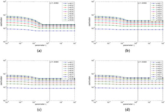
Figure 2.
Graph of the relationship between the cost function and the parameter ; varies from 0.1 to 0.9, and the original sound source signals are 200 Hz. (a) ; (b) ; (c) ; (d) .
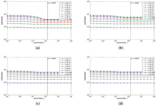
Figure 3.
Graph of the relationship between the cost function and the parameter ; varies from 0.1 to 0.9, and the original sound source signals are 500 Hz. (a) ; (b) ; (c) ; (d) .
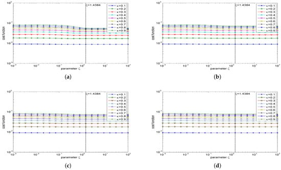
Figure 4.
Graph of the relationship between the cost function and the parameter ; varies from 0.1 to 0.9, and the original sound source signals are 800 Hz. (a) ; (b) ; (c) ; (d) .
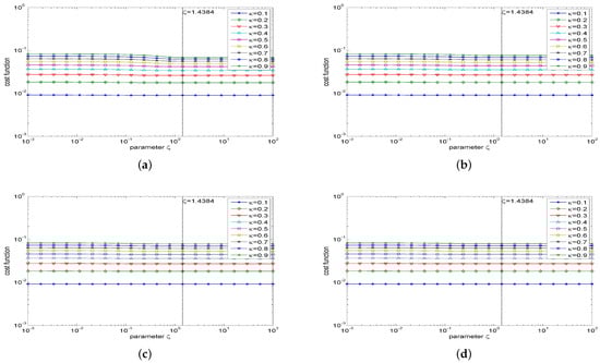
Figure 5.
Graph of the relationship between the cost function and the parameter ; varies from 0.1 to 0.9, and the original sound source signals are 1000 Hz. (a) ; (b) ; (c) ; (d) .
3.3. Quality of Sound Field Control
Reconstruction error (RE), acoustic contrast (AC), and array effort (AE) are indicators used to indicate the quality of sound field control. RE is the sound pressure error generated by the sound source and the reconstruction system in the bright zone, and its calculation formula is
AC is the ratio of the sound potential energy density of the bright region to the sound potential energy density of the dark region, which is introduced in Section 2.1; here we discretize it and take its logarithm to obtain the calculation formula as
AE is the sum of the square of loudspeakers’ distribution coefficient, calculated as follows:
The measurement criteria of these three indicators are as follows: the smaller the RE, the better the corresponding method; the larger the AC, the better the corresponding method; the smaller the AE, the better the corresponding method, and the more robust and stable the system [16].
3.4. The Selection of Parameter
Then let us choose the value of . Assuming that the source signal’s frequency ranges from 100 to 1000 Hz, the step size is 100 Hz, and changes from 0.1 to 0.9, the change step is 0.1; the relationship between the average RE, average AC, average AE, and is shown in Figure 6. From Figure 6, we can see that with the increase in , the average AC increases gradually, but the increase is relatively small; the average RE increases gradually, from −5.7584 to −1.6931 dB; the average AE decreases gradually, from −9.4790 to −20.4003 dB. Considering the measurement criteria of RE, AC, and AE comprehensively, the value of is selected as 0.1 for this example. The is because the average AC at this time is not much different from the average AC when takes other values. The average RE at this time is the smallest, and the average RE increases gradually when other values are taken, which is not good for listening experience. The average AE at this time is −9.4790 dB, which is small enough, although the average AE corresponding to other values is even smaller.
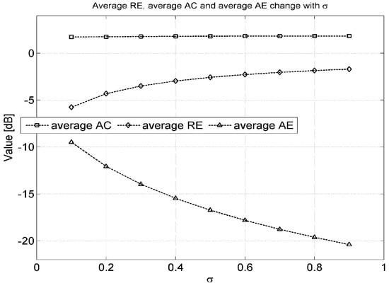
Figure 6.
Graph of the relationship between average RE, average AC, average AE, and .
4. Simulation Experiment
In this part, the performance of the proposed method is compared with that of the ACC method, the PM method in the bright zone, and the EDPM method in the bright zone in Section 2 through computer simulation experiments. In this paper, an unevenly placed five-channel system is used to verify that the proposed method can ensure the stability of the reconstruction system under the condition of ensuring relatively larger acoustic contrast and smaller reconstruction error. The relationship between the number of loudspeakers and system’s performance is not the subject of this paper.
4.1. Experiment Settings
Five loudspeakers, labeled ld 1, ld 2, …, ld 5, are placed unevenly on the same ring, and their coordinates are shown in Table 1. The loudspeaker array has a radius of 2 m. The loudspeaker array surrounds the bright zone and dark zone, which are 0.4 m in diameter. The bright zone can accommodate a listener to listen to the sound. The distance from the center point of the bright zone to the center point of the dark zone is 0.6 m. See Table 1 for the coordinates of the center points of the bright and dark zones. The origin is point O. The frequency of the original source signal changes from 100 to 1000 Hz. The original source’s location is shown in Table 1. The sound speed expressed in c is 340 m per second, the wavenumber is , and f stands for signal frequency. The sampling interval in both the bright zone and the dark zone is 0.0364 m. The relative position of the unevenly placed five-channel system is shown by Figure 7.

Table 1.
Relevant coordinates in the system.
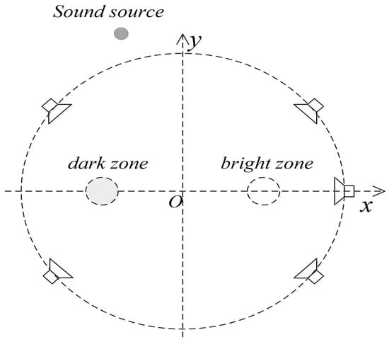
Figure 7.
Five-channel sound system structure diagram.
4.2. Experiment Results
Figure 8 shows a comparison of the acoustic contrast about four methods relative to the change with frequency. From Figure 8, we can see that the acoustic contrast of the ACC method ranges from 8.1056 to 31.1125 dB, and on the whole, different methods produce sound contrast in the order of high and low: ACC method, our method, EDPM method in the bright zone, and PM method in the bright zone. Because the goal of the ACC method is to obtain the maximum acoustic contrast, neither the EDPM method in the bright zone nor the PM method in the bright zone focuses on acoustic contrast; the proposed method controls the sound energy in the dark zone, which will improve the acoustic contrast, so the proposed method produces higher acoustic contrast than the EDPM method in the bright zone and the PM method in the bright zone. In addition to improving the acoustic contrast, the proposed method also needs to consider other factors, which affects the effect of the proposed method on acoustic contrast improvement, so the proposed method produces lower acoustic contrast than the ACC method.
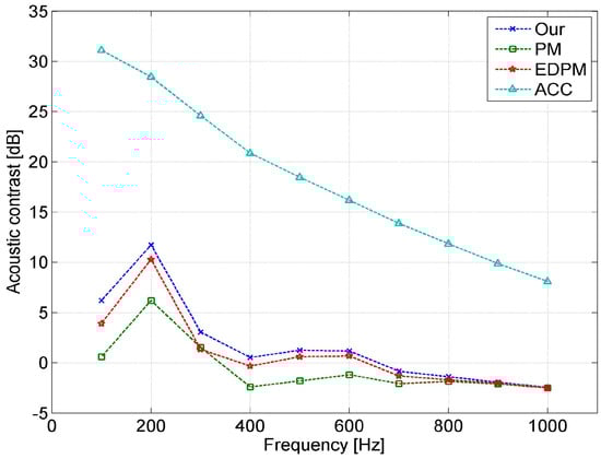
Figure 8.
Acoustic contrast comparison diagram of four methods with respect to frequency variation.
The average acoustic contrasts generated by four methods with respect to frequency are shown in Table 2. The average acoustic contrast results generated by four methods are in keeping with Figure 8. The ACC method achieves an average acoustic contrast of 18.3381 dB, the largest of all methods. The average acoustic contrast produced by our method is 2.2898 dB larger than that produced by the PM method in the bright zone and 0.8362 dB larger than that produced by the EDPM method in the bright zone.
Table 2.
Average acoustic contrast comparison of four methods with respect to frequency.
Figure 9 shows a comparison of the reconstruction error of four methods with respect to the change in frequency. The reconstruction errors of the ACC method are greater than 0 dB, which are the largest among all methods. The reconstruction errors of our method are smaller than those produced by the ACC method, and their values range from −12.2945 dB to −1.3299 dB, but are larger than those produced by the EDPM method in the bright zone and the PM method in the bright zone. The PM method in the bright zone has the smallest reconstruction error, and its values vary from −52.5606 dB to −2.0855 dB. The reason is that the goal of the PM method in the bright zone is to reduce reconstruction error as much as possible and restore the original sound field in the bright zone. The EDPM method in the bright zone is an improvement of the PM method in the bright zone in solving algorithm, and they are similar methods. The ACC method does not pay attention to reconstruction error. Our method controls reconstruction error in the bright zone, so the reconstruction errors of our method are smaller than those of the ACC method. However, our method needs to control other factors in the sound field in addition to controlling the reconstruction error in the bright zone, so the reconstruction errors of our method are larger than those of the PM method in the bright zone and the EDPM method in the bright zone.
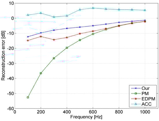
Figure 9.
Reconstruction error comparison diagram of four methods with respect to the change in frequency.
The average reconstruction errors generated by four methods with respect to frequency are shown in Table 3. The average reconstruction error results generated by different methods are consistent with Figure 9. The average reconstruction error produced by the PM method in the bright zone is −17.8140 dB, which is the smallest of all methods. The average reconstruction error produced by the ACC method is 4.3408 dB, which is the largest among all methods. The average reconstruction error produced by our method is −5.7584 dB, which is 10.0992 dB smaller than that of the ACC method, but larger than that produced by the PM method in the bright zone and the EDPM method in the bright zone.
Table 3.
Average reconstruction error comparison of different methods with respect to frequency.
Figure 10 shows a comparison of the array effort of four methods with respect to the change in frequency. The array effort produced by the ACC method is about 0 dB at 10 frequencies, which is the largest of all methods. The array efforts produced by the PM method in the bright zone are smaller than the ACC method at most frequencies, but higher than the ACC method at 100 and 200 Hz. The array efforts at all frequencies produced by the EDPM method in the bright zone are smaller than those produced by the ACC method and the PM method in the bright zone. Our method produces the lowest array efforts at all frequencies of all methods, and its value ranges from −11.8789 dB to −8.0994 dB. Our method controls array effort in the process of sound field reconstruction, while the ACC and PM methods in the bright zone and the EDPM method in the bright zone do not consider the optimization of array effort in the process of sound field reconstruction, so the array efforts generated by them are larger than those generated by our method.
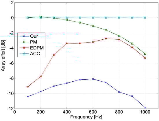
Figure 10.
Array effort diagram of four methods with respect to frequency variation.
The average array efforts generated by four methods with respect to frequency are shown in Table 4. The average array effort results generated by different methods are consistent with Figure 10. The average array effort produced by the ACC method is 0 dB, which is the largest of all methods. The average array effort produced by the other three methods is smaller than the average array effort produced by the ACC method. The average array effort produced by our method is −9.4790 dB and the smallest among all methods, which is 9.4790 dB smaller than that of the ACC method, about 8.0712 dB smaller than that of the PM method in the bright zone, and about 4.8176 dB smaller than that of the EDPM method in the bright zone.
Table 4.
Average array effort comparison of four methods with respect to frequency variation.
4.3. Discussion
Acoustic contrast, reconstruction error, and array effort are important indexes to demonstrate the sound field control ability. These three indicators are difficult to achieve the best at the same time, and there is a tradeoff relationship between them. Generally, if one of the three indicators is better for a sound field control method, the other two indicators are worse. Overall, as shown in Section 4.2 of this article, the largest acoustic contrast is obtained by the ACC method due to its focus on maximizing acoustic contrast, but it does not perform well in terms of reconstruction error and array effort; the smallest reconstruction error is achieved by the PM method in the bright zone, as it strives to minimize the reconstruction error in the bright zone, but it presents poor results in acoustic contrast and loudspeaker array effort. The EDPM method in the bright zone is similar to the PM method in the bright zone, but it has some improvements in the solving method, which is superior to the PM method in the bright zone in acoustic contrast and array effort performance, but inferior to the PM method in the bright zone in reconstruction error performance, and fails to perform better than the PM method in the bright zone in all indexes. The ACC method, PM method in the bright zone, and EDPM in the bright zone all control or optimize only one of these indexes: acoustic contrast, reconstruction error, and loudspeaker array effort, and they do not take into account the other two indexes, so they perform better in one index and poorly in the other two indexes. However, our approach is designed to reduce reconstruction error in the bright zone and loudspeaker array effort as much as possible, and to exert influence on sound pressure and particle velocity in the dark zone range. Our approach attempts to control or optimize acoustic contrast, reconstruction error, and array effort at the same time. Therefore, it is superior to the PM method in the bright zone and the EDPM method in the bright zone in terms of acoustic contrast, better than the ACC method in terms of reconstruction error, and significantly better than the ACC and PM methods in the bright zone and the EDPM method in the bright zone in terms of array effort, which can ensure the most stable reconstruction system.
5. Conclusions
Traditional sound field control technology is mainly based on sound pressure or sound pressure improvement technology, without considering another physical property of sound: particle velocity; if the loudspeaker array is placed unevenly, it will make the reconstruction system unstable. In order to solve this problem, we introduce a new sound field control method based on the traditional sound field control technology. This method pays attention to both sound pressure and particle velocity, exerts influence on the sound pressure and particle velocity in the dark zone, and tries its best to reduce the reconstruction error in the bright zone and reduce the loudspeaker array effort. The model of our method contains three weight factors: , , and , and their function and selection method are introduced in detail in this paper. Computer simulation experiments are carried out on a system with five unevenly placed loudspeaker, and our method is compared with the ACC method, PM method in the bright zone and the EDPM method in the bright zone, and the comparison indexes are reconstruction error, acoustic contrast, and loudspeaker array effort. Although the ACC method performs best in acoustic contrast and the PM method in the bright zone performs best in reconstruction error, they both focus on only one indicator and perform poorly in the other two. The EDPM method in the bright zone is an improvement of the PM method in the bright zone. Like the PM method in the bright zone, the EDPM method in the bright zone focuses on only one indicator. Although it outperforms the PM method in the bright zone on acoustic contrast and array effort, it is inferior to the PM method in the bright zone on reconstruction error. Compared with the three traditional methods, our method has the best compromise on reconstruction error, acoustic contrast, and array effort. Our method significantly outperforms other comparison methods in array effort performance. The average array effort produced by our method is about 9.4790 dB smaller than that produced by the ACC method, about 8.0712 dB smaller than that produced by the PM method in the bright zone, and about 4.8176 dB smaller than that produced by the EDPM method in the bright zone. Therefore, our method can guarantee optimal system stability in the case of uneven placement of loudspeaker array.
Author Contributions
Conceptualization, S.W.; methodology, S.W.; software, S.W.; validation, S.W.; formal analysis, C.Z.; investigation, S.W.; resources, S.W. and C.Z.; data curation, S.W.; writing—original draft preparation, S.W.; writing—review and editing, S.W. and C.Z.; visualization, S.W.; supervision, C.Z.; project administration, S.W. and C.Z.; funding acquisition, S.W. All authors have read and agreed to the published version of the manuscript.
Funding
This research was funded by the Science and Technology Research Project of the Education Department of Hubei Province (No. B2022245).
Institutional Review Board Statement
Not applicable.
Informed Consent Statement
Not applicable.
Data Availability Statement
Data are contained within the article.
Conflicts of Interest
The authors declare no conflict of interest.
References
- Yang, J.; Wu, M.; Lu, H. A review of sound field control. Appl. Sci. 2022, 12, 7319. [Google Scholar] [CrossRef]
- Choi, J.-W.; Kim, Y.-H. Generation of an acoustically bright zone with an illuminated region using multiple sources. J. Acoust. Soc. Am. 2002, 111, 1695–1700. [Google Scholar] [CrossRef] [PubMed]
- Poletti, M. An investigation of 2D multizone surround sound systems. In Proceedings of the 125th AES Convention, San Francisco, CA, USA, 2–5 October 2008. [Google Scholar]
- Coleman, P.; Jackson, P.J.B.; Olik, M.; Pedersen, J.A. Personal audio with a planar bright zone. J. Acoust. Soc. Am. 2014, 136, 1725–1735. [Google Scholar] [CrossRef] [PubMed]
- Shin, M.; Lee, S.Q.; Fazi, F.M.; Nelson, P.A.; Kim, D.; Wang, S.; Park, K.H.; Seo, J. Maximization of acoustic energy difference between two spaces. J. Acoust. Soc. Am. 2010, 128, 121–131. [Google Scholar] [CrossRef] [PubMed]
- Chang, J.-H.; Jacobsen, F. Sound field control with a circular double-layer array of loudspeakers. J. Acoust. Soc. Am. 2012, 131, 4518–4525. [Google Scholar] [CrossRef]
- Olivieri, F.; Fazi, F.M.; Shin, M.; Nelson, P. Pressure-matching beamforming method for loudspeaker arrays with frequency dependent selection of control points. In Proceedings of the 138th AES Convention, Warsaw, Poland, 7–10 May 2015. [Google Scholar]
- Afghah, T.; Patros, E.; Puckette, M. A pseudoinverse technique for the pressure-matching beamforming method. In Proceedings of the 145th AES Convention, New York, NY, USA, 17–20 October 2018. [Google Scholar]
- Elliott, S.J.; Cheer, J.; Choi, J.-W.; Kim, Y. Robustness and regularization of personal audio systems. IEEE Trans. Audio Speech Lang. Process. 2012, 20, 2123–2133. [Google Scholar] [CrossRef]
- Zhu, Q.; Coleman, P.; Wu, M.; Yang, J. Robust acoustic contrast control with reduced in-situ measurement by acoustic modeling. J. Audio Eng. Soc. 2017, 65, 460–473. [Google Scholar] [CrossRef]
- Han, Z.; Wu, M.; Zhu, Q.; Yang, J. Three-dimensional wave-domain acoustic contrast control using a circular loudspeaker array. J. Acoust. Soc. Am. 2019, 145, EL488–EL493. [Google Scholar] [CrossRef]
- Hu, M.; Lu, J. Theoretical explanation of uneven frequency response of time-domain acoustic contrast control method. J. Acoust. Soc. Am. 2021, 149, 4292–4297. [Google Scholar] [CrossRef]
- Lee, T.; Nielsen, J.K.; Christensen, M.G. Towards perceptually optimized sound zones: A proof-of-concept study. In Proceedings of the 2019 ICASSP, Brighton, UK, 12–17 May 2019; pp. 136–140. [Google Scholar]
- Lee, T.; Nielsen, J.K.; Christensen, M.G. Signal-adaptive and perceptually optimized sound zones with variable span trade-off filters. IEEE/ACM Trans. Audio Speech Lang. Process. 2020, 28, 2412–2426. [Google Scholar] [CrossRef]
- Lee, T.; Shi, L.; Nielsen, J.K.; Christensen, M.G. Fast generation of sound zones using variable span trade-off filters in the dft-domain. IEEE/ACM Trans. Audio Speech Lang. Process. 2021, 29, 363–378. [Google Scholar] [CrossRef]
- Ryu, H.; Wang, S.; Kim, S.M. Development of a personal audio performance controller with efficient, fine, and linear tunable functions. IEEE Access 2020, 8, 123916–123928. [Google Scholar] [CrossRef]
- Hu, X.; Wang, J.; Zhang, W.; Zhang, L. Time-domain sound field reproduction with pressure and particle velocity jointly controlled. Appl. Sci. 2021, 11, 10880. [Google Scholar] [CrossRef]
- Du, B.; Zeng, X.; Wang, H. A two-zone sound field reproduction based on the region energy control. In Proceedings of the Inter Noise 2021, Washington, DC, USA, 1–5 August 2021; pp. 348–354. [Google Scholar]
- Du, B.; Zeng, X.; Vorländer, M. Multizone sound field reproduction based on equivalent source method. Acoust. Aust. 2021, 49, 317–329. [Google Scholar] [CrossRef]
- Zhu, M.; Zhao, S. An iterative approach to optimize loudspeaker placement for multi-zone sound field reproduction. J. Acoust. Soc. Am. 2021, 149, 3462–3468. [Google Scholar] [CrossRef] [PubMed]
- Xie, Y.M.; Steven, G.P. A simple evolutionary procedure for structural optimization. Comput. Struct. 1993, 49, 885–896. [Google Scholar] [CrossRef]
- Zhao, S.; Burnett, I.S. Evolutionary array optimization for multizone sound field reproduction. J. Acoust. Soc. Am. 2022, 151, 2791–2801. [Google Scholar] [CrossRef]
- Zhong, J.; Zhuang, T.; Kirby, R.; Karimi, M.; Zou, H.; Qiu, X. Quiet zone generation in an acoustic free field using multiple parametric array loudspeakers. J. Acoust. Soc. Am. 2022, 151, 1235–1245. [Google Scholar] [CrossRef]
- Abe, T.; Koyama, S.; Ueno, N.; Saruwatari, H. Amplitude matching for multizone sound field control. IEEE/ACM Trans. Audio Speech Lang. Process. 2023, 31, 656–669. [Google Scholar] [CrossRef]
- Elliott, S.J.; Jones, M. An active headrest for personal audio. J. Acoust. Soc. Am. 2006, 119, 2702–2709. [Google Scholar] [CrossRef]
- Cheer, J.; Elliott, S.J.; Kim, Y. Practical implementation of personal audio in a mobile device. J. Audio Eng. Soc. 2013, 61, 290–300. [Google Scholar]
- Cheer, J.; Elliott, S.J.; Gálvez, M.F.S. Design and implementation of a car cabin personal audio system. J. Audio Eng. Soc. 2013, 61, 412–424. [Google Scholar]
- Liao, X.; Cheer, J.; Elliott, S.J.; Zheng, S. Design of a loudspeaker array for personal audio in a car cabin. J. Audio Eng. Soc. 2017, 65, 226–238. [Google Scholar] [CrossRef]
- Choi, J.W. Real-Time demonstration of personal audio and 3D audio rendering using line array systems. In Proceedings of the MMM 2020, Daejeon, Republic of Korea, 5–8 January 2020. [Google Scholar]
- Pierce, A.D. Acoustics, an Introduction to Its Physical Principles and Applications; Acoustical Society of America: New York, NY, USA, 1989. [Google Scholar]
- Shin, M.; Nelson, P.A.; Fazi, F.M.; Seo, J. Velocity controlled sound field reproduction by non-uniformly spaced loudspeakers. J. Sound Vib. 2016, 370, 444–464. [Google Scholar] [CrossRef]
- Olivieri, F.; Fazi, F.M.; Nelson, P.A.; Fontana, S. Comparison of strategies for accurate reproduction of a target signal with compact arrays of loudspeakers for the generation of zones of private sound and silence. J. Audio Eng. Soc. 2016, 64, 905–917. [Google Scholar] [CrossRef]
- Grant, M.; Boyd, S. CVX, Version 1.21 MATLAB Toolbox for Disciplined Convex Programming. Available online: http://cvxr.com/cvx (accessed on 5 November 2023).
- Bai, M.R.; Chen, C.C. Application of convex optimization to acoustical array signal processing. J. Sound Vib 2013, 332, 6596–6616. [Google Scholar] [CrossRef]
- Grant, M.; Boyd, S.; Ye, Y. Disciplined convex programming. In Global Optimization: From Theory to Implementation, Nonconvex Optimization and Applications; Liberti, L., Maculan, N., Eds.; Springer: New York, NY, USA, 2006; pp. 155–210. [Google Scholar]
Disclaimer/Publisher’s Note: The statements, opinions and data contained in all publications are solely those of the individual author(s) and contributor(s) and not of MDPI and/or the editor(s). MDPI and/or the editor(s) disclaim responsibility for any injury to people or property resulting from any ideas, methods, instructions or products referred to in the content. |
© 2023 by the authors. Licensee MDPI, Basel, Switzerland. This article is an open access article distributed under the terms and conditions of the Creative Commons Attribution (CC BY) license (https://creativecommons.org/licenses/by/4.0/).