
Flexible Job Shop Scheduling Optimization for Green Manufacturing Based on Improved Multi-Objective Wolf Pack Algorithm


Abstract
:1. Introduction
2. Problem Description and Modeling
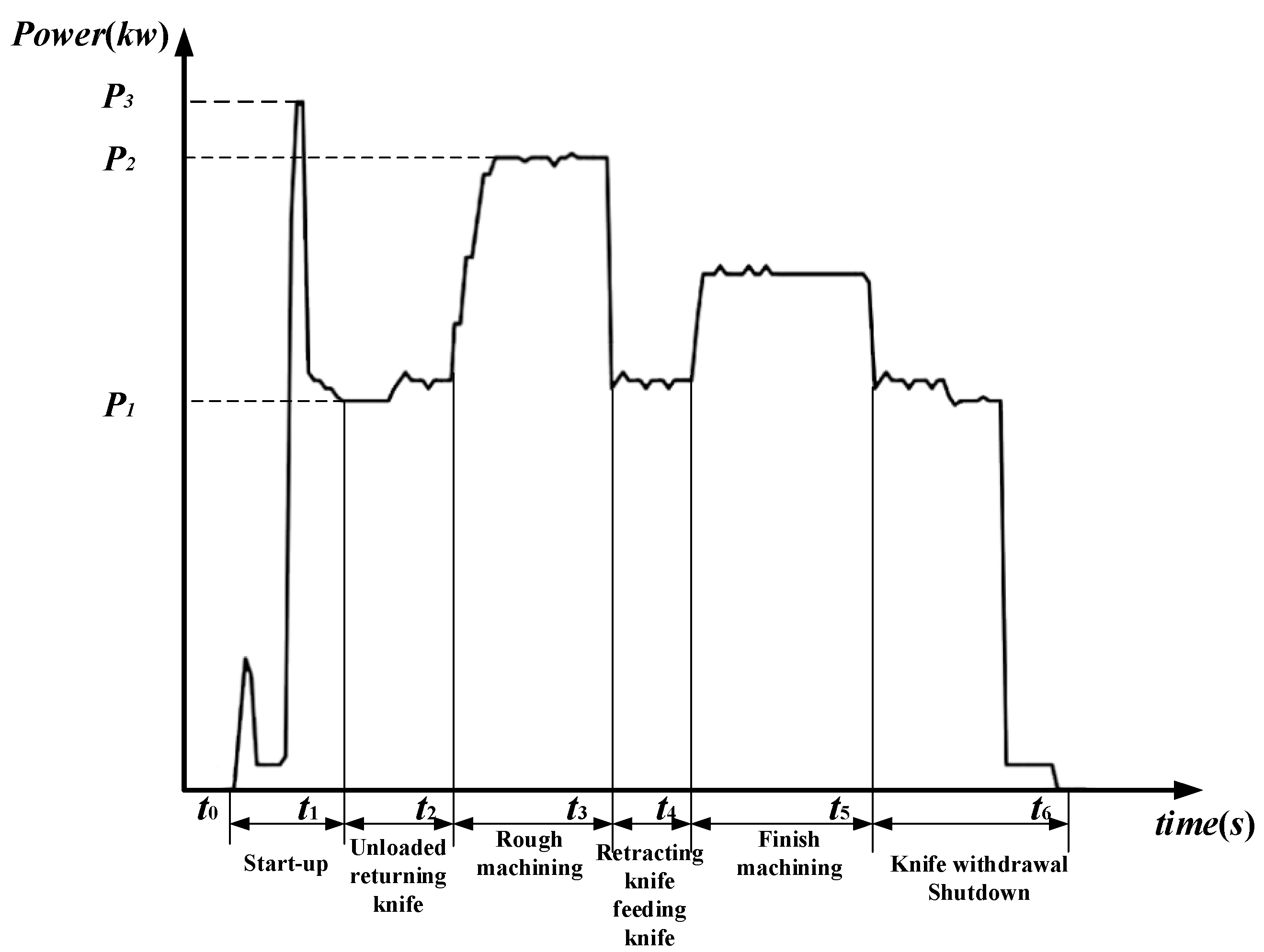
2.1. Problem Description
- (1)
- Each workpiece must be processed in the previous process before it can be processed in the next process;
- (2)
- Each process of each workpiece can only be processed on one machine;
- (3)
- The workpiece will not be interrupted during processing;
- (4)
- At the same time, each machine can only process one workpiece, and each workpiece can only be processed by one machine;
- (5)
- At the initial moment, all workpieces and machines are ready;
- (6)
- For the first process of each workpiece, transportation time and energy consumption are not considered;
- (7)
- The idle start time of each machine is the end time of the last process, and the idle end time is the start time of the first process;
- (8)
- During the transportation of workpieces, problems such as transportation failures are not considered.
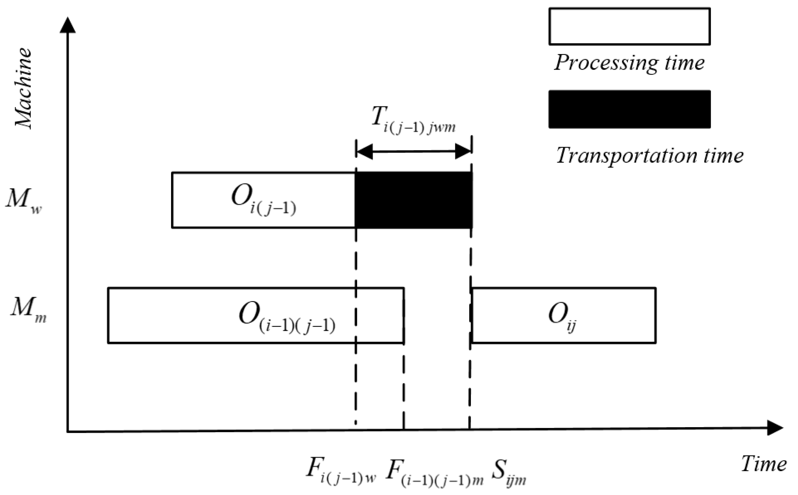
2.2. Mathematical Model Building
3. Improved Multi-Objective Wolf Pack Algorithm Design
3.1. Encoding and Decoding
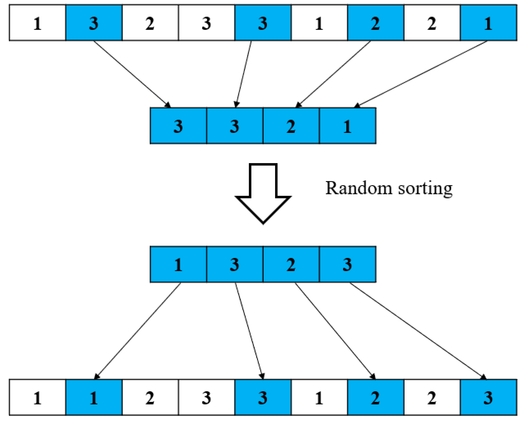
3.2. Population Initialization
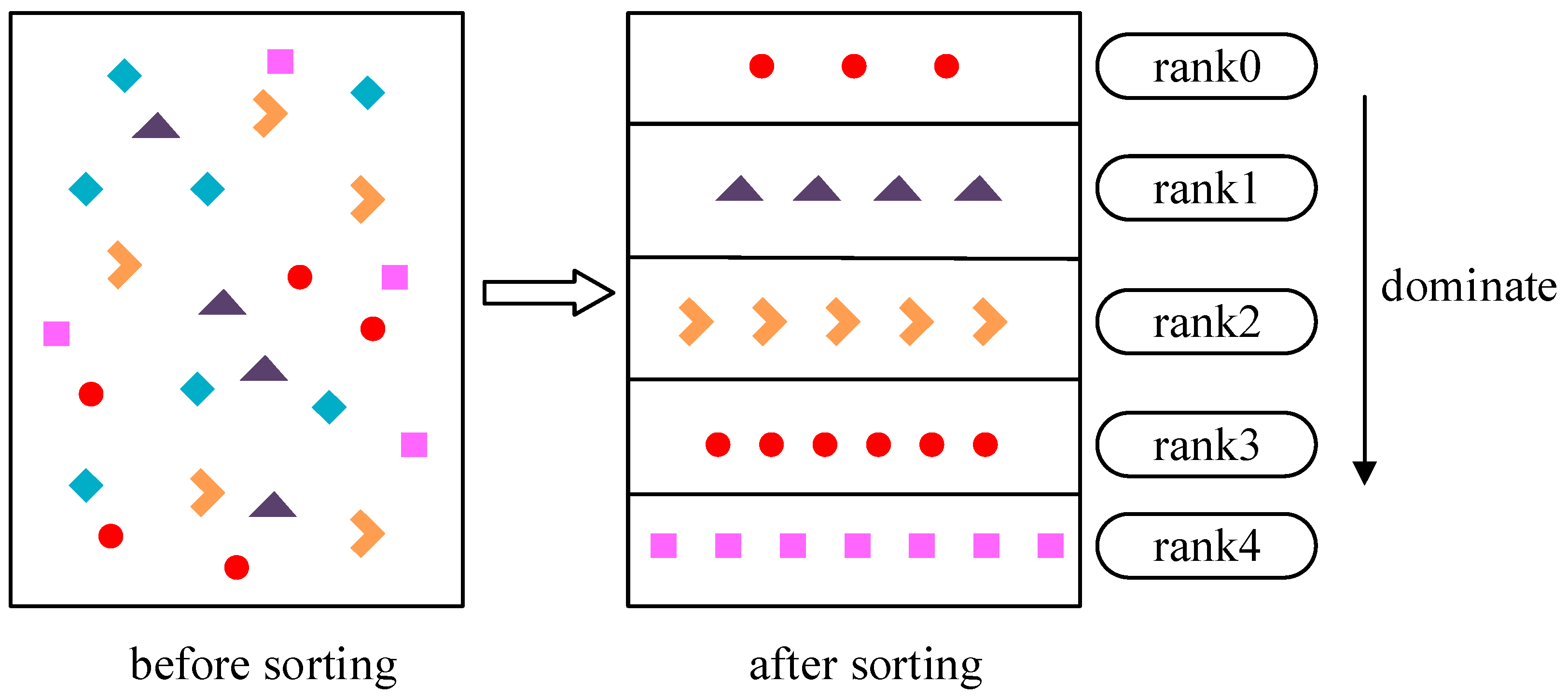
3.3. Non-Dominated Crowding Ranking
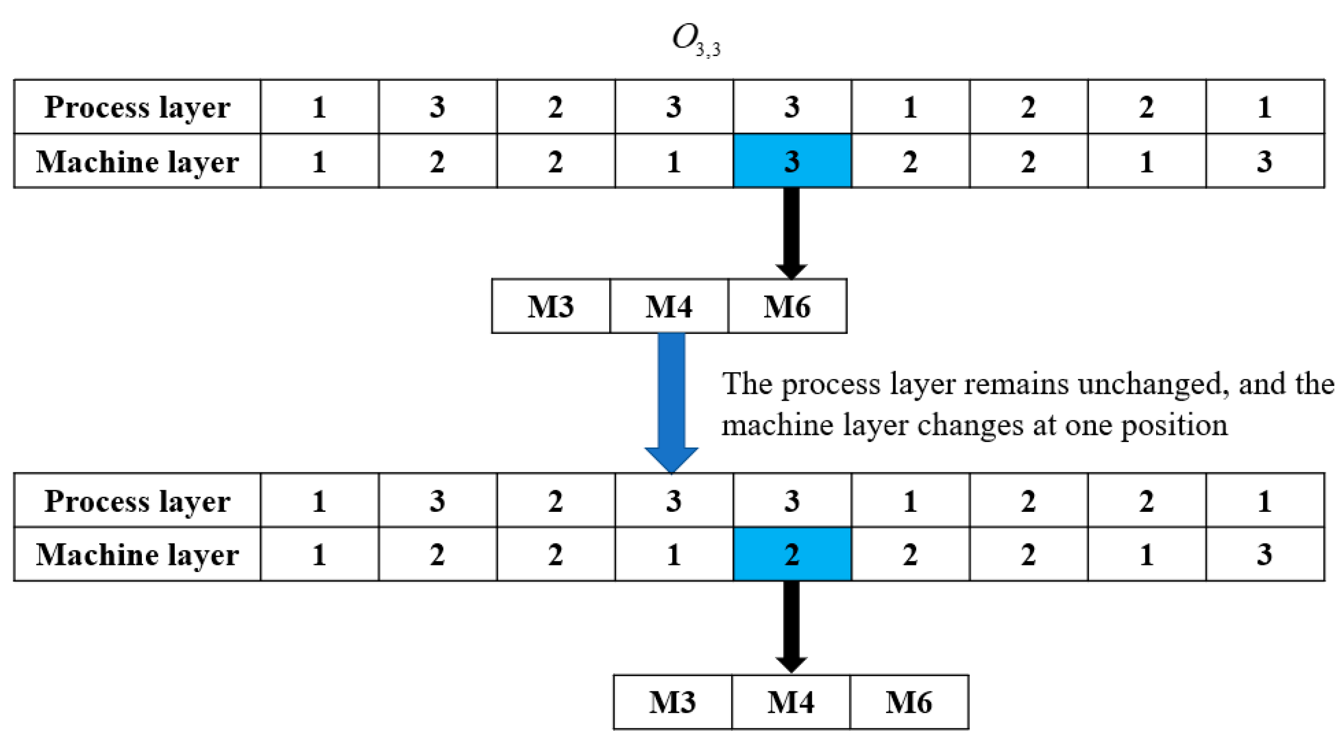
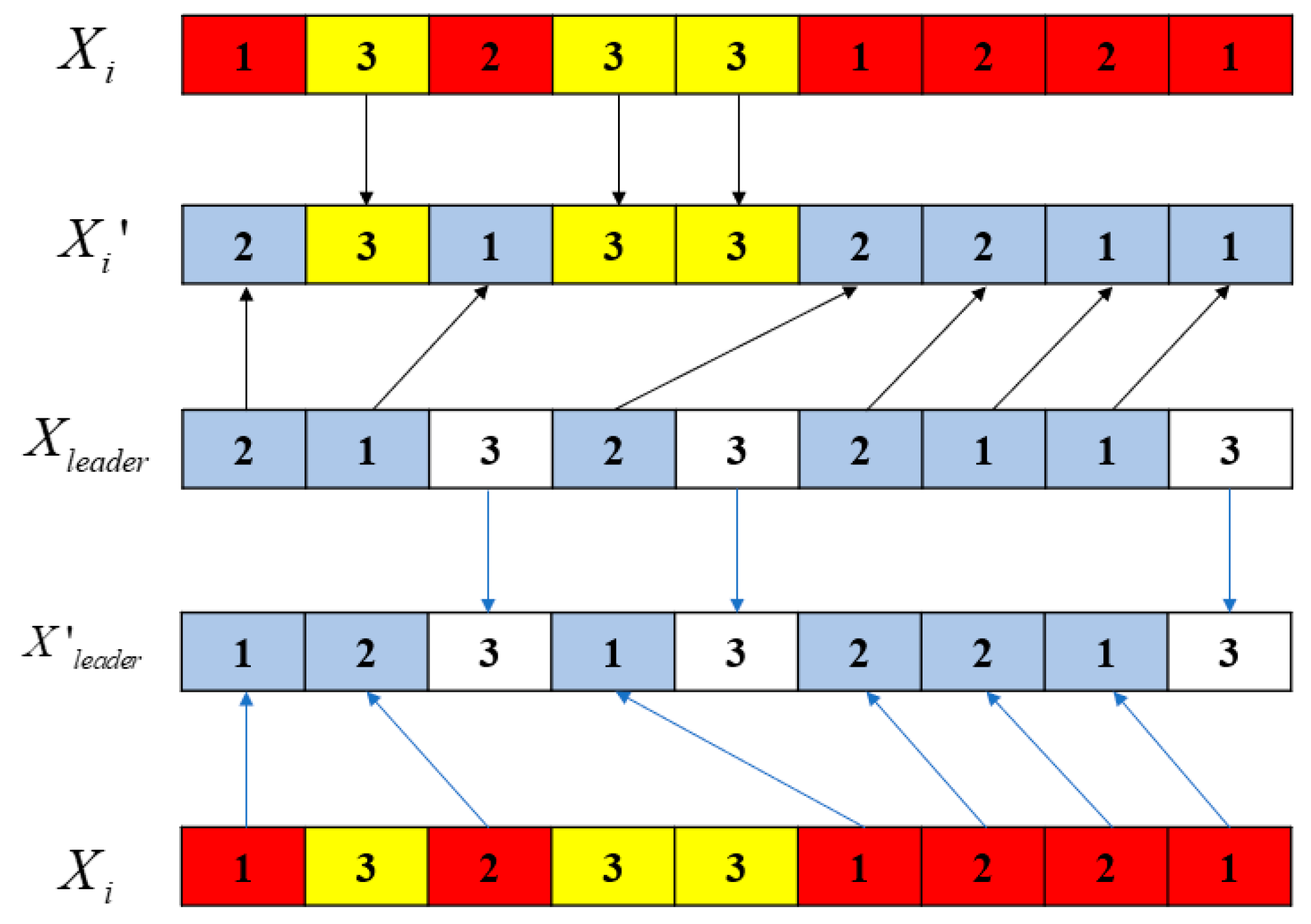
3.4. Intelligent Behavior Design
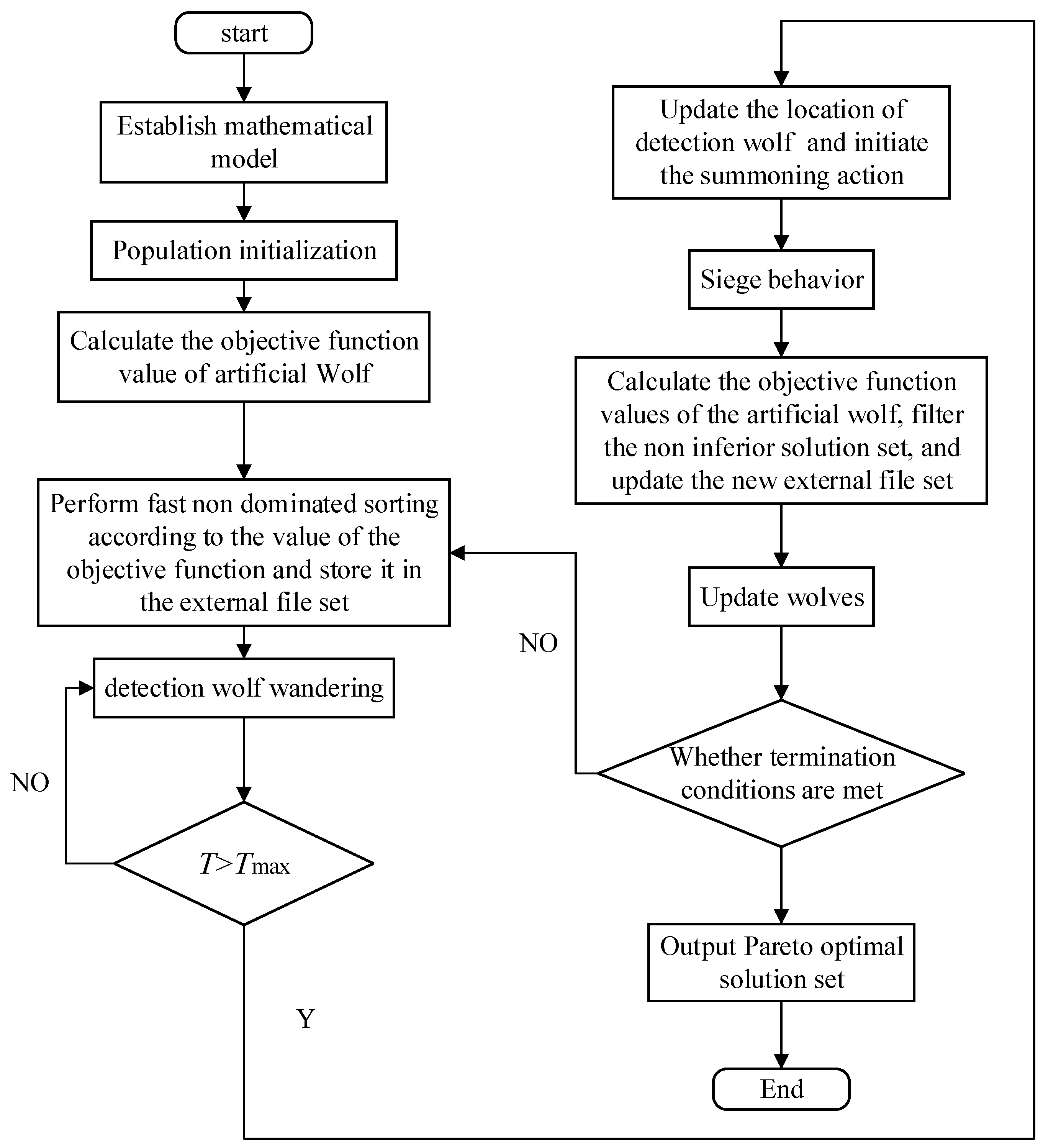
3.5. Algorithm Flow
4. Simulation Testing and Analysis
4.1. Test Example
4.2. Selection of Pareto Optimal Solution Set
- (1)
- Calculate the weight value
- (2)
- Data normalization
- (3)
- Calculation of gray correlation coefficient
- (4)
- Calculation of gray correlation degree
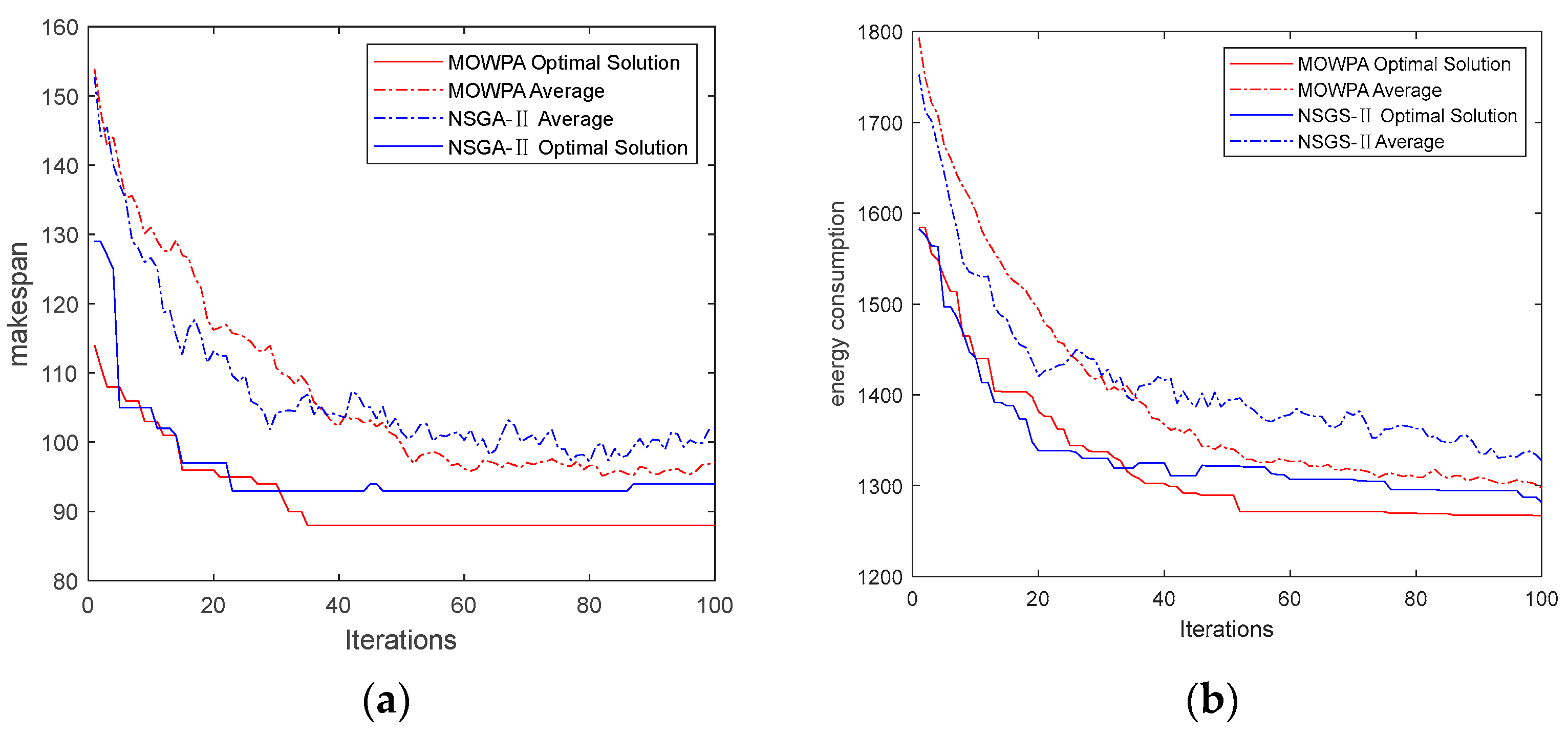
4.3. Algorithm Performance Evaluation
5. Conclusions
Author Contributions
Funding
Institutional Review Board Statement
Informed Consent Statement
Data Availability Statement
Conflicts of Interest
References
- Garey, M.R.; Sethi, J.R. The complexity of flow shop and job shop scheduling. Math. Oper. Res. 1976, 1, 117–129. [Google Scholar] [CrossRef]
- Shen, L.; Dauzère, P.; Stéphane; Neufeld, J.S. Solving the flexible job shop scheduling problem with sequence-dependent setup times. Eur. J. Oper. Res. 2018, 265, 503–516. [Google Scholar] [CrossRef]
- Homayouni, S.M.; Fontes, D.; Gonalves, J.F. A multistart biased random key genetic algorithm for the flexible job shop scheduling problem with transportation. Int. Trans. Oper. Res. 2020, 30, 688–716. [Google Scholar] [CrossRef]
- Peng, K.; Pan, Q.K.; Gao, L.; Li, X.; Das, S.; Zhang, B. A multi-start variable neighbourhood descent algorithm for hybrid flow shop rescheduling. Swarm Evol. Comput. 2019, 45, 92–112. [Google Scholar] [CrossRef]
- An, Y.; Chen, X.; Zhang, J.; Li, Y. A hybrid multi-objective evolutionary algorithm to integrate optimization of the production scheduling and imperfect cutting tool maintenance considering total energy consumption. J. Clean. Prod. 2020, 268, 121540. [Google Scholar] [CrossRef]
- Zheng, X.; Wang, L. A Collaborative Multiobjective Fruit Fly Optimization Algorithm for the Resource Constrained Unrelated Parallel Machine Green Scheduling Problem. IEEE Trans. Syst. Man Cybern. Syst. 2018, 48, 790–800. [Google Scholar] [CrossRef]
- Luo, S.; Zhang, L.; Fan, Y. Energy-efficient scheduling for multi-objective flexible job shops with variable processing speeds by grey wolf optimization. J. Clean. Prod. 2019, 234, 1365–1384. [Google Scholar] [CrossRef]
- Wu, X.; Sun, Y. A Green Scheduling Algorithm for Flexible Job Shop with Energy-Saving Measures. J. Clean. Prod. 2018, 172 Pt 3, 3249–3264. [Google Scholar] [CrossRef]
- Peng, Z.; Zhang, H.; Tang, H.; Feng, Y.; Yin, W. Research on flexible job-shop scheduling problem in green sustainable manufacturing based on learning effect. J. Intell. Manuf. 2022, 33, 1725–1746. [Google Scholar] [CrossRef]
- Hasani, A.; Hosseini, S. A bi-objective flexible flow shop scheduling problem with machine-dependent processing stages: Trade-off between production costs and energy consumption. Appl. Math. Comput. 2020, 386, 125533. [Google Scholar] [CrossRef]
- Zhu, Z.; Zhou, X. An efficient evolutionary grey wolf optimizer for multi-objective flexible job shop scheduling problem with hierarchical job precedence constraints. Comput. Ind. Eng. 2020, 140, 106280. [Google Scholar] [CrossRef]
- Caldeira, R.H.; Gnanavelbabu, A. A Pareto based discrete Jaya algorithm for multi-objective flexible job shop scheduling problem. Expert Syst. Appl. 2021, 170, 114567. [Google Scholar] [CrossRef]
- Kui, C.; Li, B. Research on FJSP based on improved particle swarm optimization algorithm considering transportation time. J. Syst. Simul. 2021, 4, 845–853. [Google Scholar]
- Xiabao, H.; Shuling, W. High dimensional multi-objective flexible job shop scheduling considering low carbon. J. Wuhan Univ. Technol. Inf. Manag. Eng. Ed. 2019, 41, 592–598. [Google Scholar]
- Foumani, M.; Smith-miles, K. The impact of various carbon reduction policies on green flowshop scheduling. Appl. Energy 2019, 249, 300–315. [Google Scholar] [CrossRef]
- Chen, W.; Wang, J.; Yu, G.; Hu, Y. Energy-Efficient Hybrid Flow-Shop Scheduling under Time-of-Use and Ladder Electricity Tariffs. Appl. Sci. 2022, 12, 6456. [Google Scholar] [CrossRef]
- Liu, Z.; Guo, S.; Wang, L. Integrated green scheduling optimization of flexible job shop and crane transportation considering comprehensive energy consumption. J. Clean. Prod. 2019, 211, 765–786. [Google Scholar] [CrossRef]
- Chen, X.; Cheng, F.; Liu, C.; Cheng, L.; Mao, Y. An improved Wolf pack algorithm for optimization problems: Design and evaluation. PLoS ONE 2021, 16, e0254239. [Google Scholar] [CrossRef]
- Yong, Y.; Huizhen, Z. Wolf swarm algorithm for vehicle routing problem with multiple distribution centers. Comput. Appl. Res. 2017, 34, 2590–2593. [Google Scholar]
- Shan, G.; Meng, L. Greedy stochastic adaptive gray wolf optimization algorithm for solving TSP problems. Mod. Electron. Technol. 2019, 42, 50–54. [Google Scholar]
- Liwen, W.; Shuyi, S.; Qingxian, W.; Zengliang, H. Unmanned Helicopter Trajectory Planning Based on Improved Wolf Pack Algorithm. Systems Engineering and Electronics Technology 2023.07.22. Available online: http://kns.cnki.net/kcms/detail/11.2422.TN.20221228.1122.005.htm (accessed on 17 June 2023).
- Shikui, Z. Two-Level Neighborhood Search Hybrid Algorithm for Flexible Workshop Scheduling Problem. J. Mech. Eng. 2015, 51, 175–184. [Google Scholar]
- Jinliang, S.; Fei, L.; Dijian, X.; Guorong, C. Energy-saving Decision-making Model and Practical Method of CNC Machine Tool in No-load Operation. China Mach. Eng. 2009, 20, 1344–1346. [Google Scholar]
- Husheng, W.; Fengming, Z.; Lushan, W. A new swarm intelligence algorithm—The wolf swarm algorithm. Syst. Eng. Electron. Technol. 2013, 35, 2430–2438. [Google Scholar]
- Chaoyong, Z.; Yunqing, R.; Xiangjun, L.; Peigen, L. A Genetic Algorithm Based on POX Intersection for Solving Jobs Shop Scheduling Problem. China Mech. Eng. 2004, 23, 83–87. [Google Scholar]
- Brandimarte, P. Routing and scheduling in a flexible job shop by tabu search. Ann. Oper. Res. 1993, 41, 157–183. [Google Scholar] [CrossRef]
- Czyzzak, P.; Jaszkiewicz, A. Pareto simulated annealing—A metaheuristic technique for multiple-objective combinatorial optimization. J. Multi-Criteria Decis. Anal. 1998, 7, 34–47. [Google Scholar] [CrossRef]


| Symbols | Definitions | |
|---|---|---|
| Parameters | Workpieces | |
| Working sequence | ||
| Machines | ||
| The j-th process of the i-th workpiece | ||
| Processing time of on machine k | ||
| Time for transporting N from machine tool to machine tool between operation and of workpiece N | ||
| Integer variable, takes 0 or 1 if is processed on machine k, otherwise 0 | ||
| Machining power of machine tool k | ||
| Standby power of machine tool k | ||
| Power for transporting N from machine tool to machine tool between operation and of workpiece N | ||
| Variables | Starting processing time of at machine k | |
| end processing time on machine k | ||
| Completion time for workpiece i | ||
| Machining time of machine tool k | ||
| Standby time of machine tool k | ||
| Total energy consumption of machine tool k | ||
| Machining energy consumption of machine tool k | ||
| Standby energy consumption of machine tool k | ||
| Total transportation energy consumption |
| Process layer | 1 | 1 | 2 | 3 | 3 | 1 | 2 | 2 | 3 |
| Machine layer | 1 | 2 | 2 | 1 | 2 | 2 | 2 | 1 | 3 |
| Machine Power | ||||||||||
|---|---|---|---|---|---|---|---|---|---|---|
| Processing power | 2 | 1.8 | 1.6 | 2.4 | 2.4 | 4.1 | 3.5 | 4.1 | 2.8 | 2.7 |
| standby power | 0.5 | 0.6 | 0.3 | 0.4 | 0.4 | 0.6 | 0.8 | 0.9 | 0.3 | 0.4 |
| Machines | ||||||||||
|---|---|---|---|---|---|---|---|---|---|---|
| 0 | 2 | 1 | 2 | 4 | 3 | 4 | 3 | 2 | 3 | |
| 2 | 0 | 2 | 2 | 3 | 2 | 3 | 4 | 4 | 2 | |
| 1 | 2 | 0 | 3 | 2 | 4 | 3 | 1 | 5 | 2 | |
| 2 | 2 | 3 | 0 | 4 | 4 | 3 | 4 | 3 | 2 | |
| 4 | 3 | 2 | 4 | 0 | 1 | 4 | 4 | 3 | 4 | |
| 3 | 2 | 4 | 4 | 1 | 0 | 4 | 3 | 2 | 2 | |
| 4 | 3 | 3 | 3 | 4 | 4 | 0 | 5 | 1 | 3 | |
| 3 | 4 | 1 | 4 | 4 | 3 | 5 | 0 | 4 | 1 | |
| 2 | 4 | 5 | 3 | 3 | 2 | 1 | 4 | 0 | 3 | |
| 3 | 2 | 2 | 2 | 4 | 2 | 3 | 1 | 3 | 0 |
| Parameter Name | Numerical Value |
|---|---|
| Population number | 200 |
| Iterations | 100 |
| External archive collection size | 100 |
| Maximum number of walking | 10 |
| Procedure walking step | 6 |
| Machine Walking Steps | 4 |
| Siege steps | 6 |
| Detection wolf scale factor | 0.4 |
| Update scale factor | 0.3 |
| Serial Number | Energy Consumption of Each Part | ||||
|---|---|---|---|---|---|
| Transportation Energy Consumption | Processing Energy Consumption | Standby Energy Consumption | |||
| 1 | 87 | 1332.60 | 359.10 | 856.50 | 117.00 |
| 2 | 89 | 1320.76 | 347.76 | 854.60 | 118.40 |
| 3 | 90 | 1311.08 | 343.98 | 836.50 | 130.60 |
| 4 | 91 | 1300.91 | 357.21 | 836.20 | 130.50 |
| 5 | 92 | 1270.43 | 334.53 | 828.70 | 107.20 |
| 6 | 93 | 1267.99 | 342.09 | 826.80 | 99.10 |
| 7 | 94 | 1259.91 | 338.31 | 824.60 | 97.00 |
| 8 | 95 | 1242.32 | 336.42 | 805.10 | 100.80 |
| 9 | 100 | 1219.09 | 323.19 | 765.50 | 130.40 |
| 10 | 101 | 1210.43 | 320.53 | 763.30 | 126.60 |
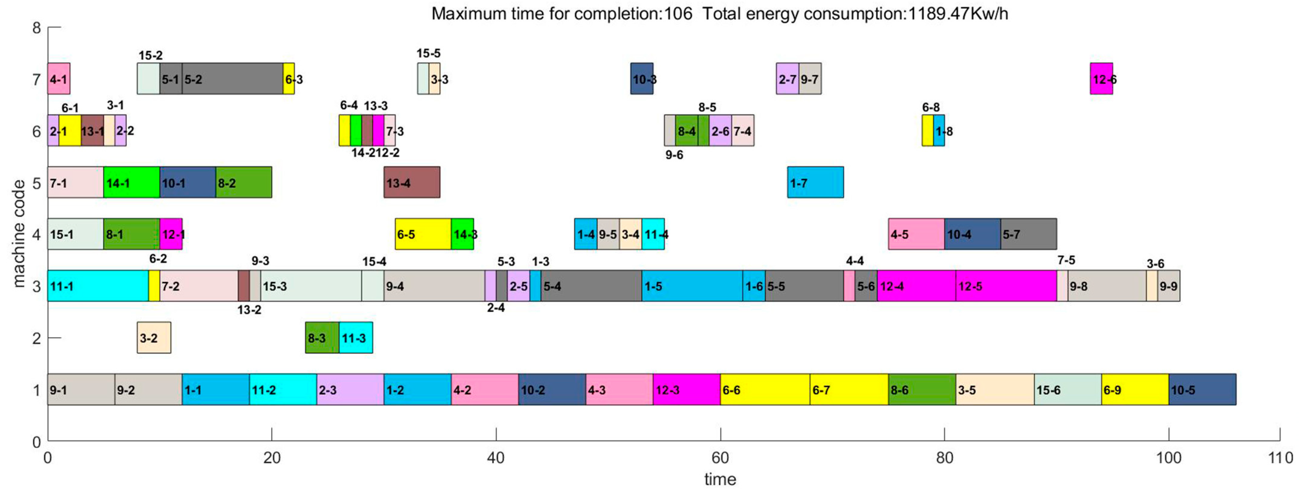
| 11 | 106 | 1189.47 | 308.07 | 743.80 | 137.60 |
| Indicators | Weights | ||
|---|---|---|---|
| 1 | 1/2 | 1/3 | |
| 2 | 1 | 2/3 |
| Test Data | The Set of Pareto Solutions Obtained by MOWPA | The Set of Pareto Solutions Obtained by NSGA-II |
|---|---|---|
| MK01 | (46;525.53), (52;516.62), (58;513.43) (47;522.11), (51;518), (45;526.91) (44;530) | (49;546.97), (50;539.37), (51;532.77) (52;524.79), (58;501.11) |
| MK02 | (37;526.91), (38;519.49), (39;514.91) (40;513.09), (41;512.51), (42;512.11) (43;511.47), (44;510.89), (45;509.49) | (38;539.11), (39;534.44), (40;530.68) (43;527.56), (44;522.98) |
| MK03 | (208;3,452.10), (209;3,430.66) (212;3,418.42), (213;3,399.43) (215;3,384.83) | (210;3,462.53), (211;3,439.23) (214;3,410.55), (217;3,398.75) (218;3,375.26) |
| MK04 | (87;1,332.6), (89;1,320.76), (90;1,311.08) (91;1,300.91), (92;1,270.43), (93;1,267.99) (94;1,259.91), (95;1,242.32) (100;1,219.09), (101;1,210.43) (110;1,189.47) | (89;1,357.97), (93;1,337.47), (94;1,313.83) (100;1,289.51), (102;1,276.07), (104;1,259.23) (109;1,251.44) |
| MK05 | (180;1,632.63), (183;1,630.21) (185;1,626.91), (186;1,624.62) (189;1,623.4) | (182;1,669.95), (183;1,652.78) (184;1,644.08), (186;1,625.29) |
| MK06 | (108;1,740.01), (109;1,719.93) (110;1,699.66), (111;1,696.25) (112;1,689.56), (113;1,688.45) (114;1,685.01), (115;1,683.09) | (108;1,799.12), (109;1,750.59) (110;1,740.88), (112;1,730.54) (113;1,720.03), (115;1,690.67) |
| MK07 | (144;1,745.22), (145;1,738.03) (146;1,735.03), (150;1,730.65) (155;1,724.42), (160;1,720.72) (162;1,719.44) | (146;1,766.53), (147;1,754.86) (149;1,750.31), (150;1,743.33) |
| Test Data | C (MOWPA, NSGA-II) | IGD (MOWPA) | IGD (NSGA-II) |
|---|---|---|---|
| MK01 | 1.00 | 1.2070 | 4.8498 |
| MK02 | 1.00 | 1.3956 | 1.2903 |
| MK03 | 0.60 | 1.1363 | 2.3480 |
| MK04 | 1.00 | 3.9281 | 4.5960 |
| MK05 | 1.00 | 0.5362 | 3.0486 |
| MK06 | 1.00 | 3.6433 | 8.4704 |
| MK07 | 1.00 | 1.5487 | 0.8967 |
Disclaimer/Publisher’s Note: The statements, opinions and data contained in all publications are solely those of the individual author(s) and contributor(s) and not of MDPI and/or the editor(s). MDPI and/or the editor(s) disclaim responsibility for any injury to people or property resulting from any ideas, methods, instructions or products referred to in the content. |
© 2023 by the authors. Licensee MDPI, Basel, Switzerland. This article is an open access article distributed under the terms and conditions of the Creative Commons Attribution (CC BY) license (https://creativecommons.org/licenses/by/4.0/).
Share and Cite
Li, J.; Li, H.; He, P.; Xu, L.; He, K.; Liu, S. Flexible Job Shop Scheduling Optimization for Green Manufacturing Based on Improved Multi-Objective Wolf Pack Algorithm. Appl. Sci. 2023, 13, 8535. https://doi.org/10.3390/app13148535
Li J, Li H, He P, Xu L, He K, Liu S. Flexible Job Shop Scheduling Optimization for Green Manufacturing Based on Improved Multi-Objective Wolf Pack Algorithm. Applied Sciences. 2023; 13(14):8535. https://doi.org/10.3390/app13148535
Chicago/Turabian StyleLi, Jian, Huankun Li, Pengbo He, Liping Xu, Kui He, and Shanhui Liu. 2023. "Flexible Job Shop Scheduling Optimization for Green Manufacturing Based on Improved Multi-Objective Wolf Pack Algorithm" Applied Sciences 13, no. 14: 8535. https://doi.org/10.3390/app13148535
APA StyleLi, J., Li, H., He, P., Xu, L., He, K., & Liu, S. (2023). Flexible Job Shop Scheduling Optimization for Green Manufacturing Based on Improved Multi-Objective Wolf Pack Algorithm. Applied Sciences, 13(14), 8535. https://doi.org/10.3390/app13148535