Article

Machine Learning Techniques for Soil Characterization Using Cone Penetration Test Data

by
Ayele Tesema Chala
* and
Richard P. Ray
*
Structural and Geotechnical Engineering Department, Faculty of Architecture, Civil and Transport Sciences, Szechenyi Istvan University, H-9026, Egyetem Ter 1, 9026 Gyor, Hungary
*
Authors to whom correspondence should be addressed.
Appl. Sci. 2023, 13(14), 8286; https://doi.org/10.3390/app13148286
Submission received: 6 June 2023 / Revised: 10 July 2023 / Accepted: 13 July 2023 / Published: 18 July 2023
(This article belongs to the Special Issue The Application of Machine Learning in Geotechnical Engineering)

Abstract

:
Seismic response assessment requires reliable information about subsurface conditions, including soil shear wave velocity ( V s ) . To properly assess seismic response, engineers need accurate information about V s , an essential parameter for evaluating the propagation of seismic waves. However, measuring V s is generally challenging due to the complex and time-consuming nature of field and laboratory tests. This study aims to predict V s using machine learning (ML) algorithms from cone penetration test (CPT) data. The study utilized four ML algorithms, namely Random Forests (RFs), Support Vector Machine (SVM), Decision Trees (DT), and eXtreme Gradient Boosting (XGBoost), to predict V s . These ML models were trained on 70% of the datasets, while their efficiency and generalization ability were assessed on the remaining 30%. The hyperparameters for each ML model were fine-tuned through Bayesian optimization with k-fold cross-validation techniques. The performance of each ML model was evaluated using eight different metrics, including root mean squared error (RMSE), mean absolute error (MAE), mean absolute percentage error (MAPE), coefficient of determination ( R 2 ), performance index ( P I ), scatter index ( S I ), A 10 I , and U 95 . The results demonstrated that the RF model consistently performed well across all metrics. It achieved high accuracy and the lowest level of errors, indicating superior accuracy and precision in predicting V s . The SVM and XGBoost models also exhibited strong performance, with slightly higher error metrics compared with the RF model. However, the DT model performed poorly, with higher error rates and uncertainty in predicting V s . Based on these results, we can conclude that the RF model is highly effective at accurately predicting V s using CPT data with minimal input features.

1. Introduction

Soil characterization plays a vital role in seismic response assessment and interpreting subsurface conditions for large-scale engineering projects. To properly assess seismic response, engineers need accurate and reliable information about subsurface conditions, including soil shear wave velocity ( V s ), an essential parameter for evaluating the propagation of seismic waves [1,2,3,4,5,6]. Seismic-refraction and reflection methods using geophysical signal processing [7,8,9,10] measure V s at various depths and precision to produce a profile (preferably to bedrock) for later analysis. To measure V s , an active source generates a wave and its travel time to one or more receivers is measured. The velocity results from knowing the time and distance traveled between the source and receiver. There are several V s measurement methods, including seismic cone penetration testing (SCPT) [7], Multi-Channel Analysis of Surface Waves (MASW) [8], Cross-hole testing [8], and down-hole testing methods. These techniques provide valuable information about subsurface conditions but become more complex with increasing soil layering.
Additionally, laboratory tests such as bender element [11], triaxial test [12], and resonant column tests [13] measure V s in different ways. These tests are conducted on soil samples collected from the site and offer a controlled environment for testing, providing detailed information on soil behavior under varying stress conditions. However, retrieving high-quality intact soil samples is a challenging task that requires specialist equipment [14]. Furthermore, it is important to note that the properties of collected samples may significantly change over time due to variations in stress conditions, temperature fluctuations, and moisture content.
A viable alternative is to correlate V s to cone penetration test (CPT) data, a relatively easier approach. Many empirical correlations have been developed over the past couple of decades to estimate V s from CPT data [15,16,17,18,19]. The CPT test involves pushing a cone-shaped instrument into the ground at a constant rate while measuring the resistance of the soil. Two measurements are typically taken during this test: cone tip resistance ( q c ) and sleeve friction ( f s ) [20,21]. The CPT test provides continuous and reliable soil data, making it an efficient and cost-effective method in geotechnical engineering practice. This wealth of CPT data has attracted the attention of many geotechnical researchers to further improve the prediction accuracy of V s employing machine learning (ML) algorithms [22,23,24,25,26]. ML algorithms have shown great promise in accurately predicting V s from CPT data. The ML algorithms can learn complex relationships between input variables (e.g., q c and f s records) and output variables (e.g., soil V s ) from large datasets without the need for explicit mathematical models.
Many ML algorithms, such as gradient boosting, random forest, support vector machine (SVM) artificial neural network (ANN), and decision trees (DT), have been used in various geotechnical applications, including soil classification [27,28,29,30,31,32,33], V s prediction [23,24,25,26,34], liquefaction analysis [35,36,37,38,39,40], stability analysis [41,42,43,44,45], and settlement prediction [46,47,48]. The application of ML algorithms in geotechnical engineering has shown promising results in terms of efficiency and accuracy. For example, Tsiaousi et al. [25] successfully employed an ANN model to characterize soil stratigraphy and predict V s . This study demonstrates how ML approaches can be used to improve soil characterization and prediction of important geotechnical parameters. Assaf et al. [24] and Riyadi et al. [49] have also used ML algorithms, including RF and XGBoost, to predict V s . Their findings confirm that ML models can achieve high accuracy and performance in predicting V s . Previous research has also shown that SVM performs well in predicting V s [50,51]. These studies collectively demonstrate the potential of ML algorithms in improving the accuracy of V s prediction in geotechnical engineering applications.
The aim of this study is to improve the prediction of V s using various ML algorithms with minimal input features. Four ML algorithms, namely RF, SVM, DT, and eXtreme gradient boosting (XGBoost), are employed to predict V s from CPT data. The study also aims to minimize the need for expensive and time-consuming fields or laboratory measurements. The development of ML models can lead to higher accuracy and performance in predicting V s . The improvement in the accuracy of V s prediction has significant implications for site response assessment and seismic risk reduction. By utilizing ML to predict V S , this study has the potential to enhance existing knowledge and inspire future research in the field of ML applications for soil characterization.
The rest of this document is organized as follows: Section 2 discusses dataset preprocessing and visualization, Methodology and performance metrics are described in Section 3, Section 4 describes the ML models, and Section 5 presents the results. Finally, Section 6 outlines the main results of the study and concludes by suggesting future research.

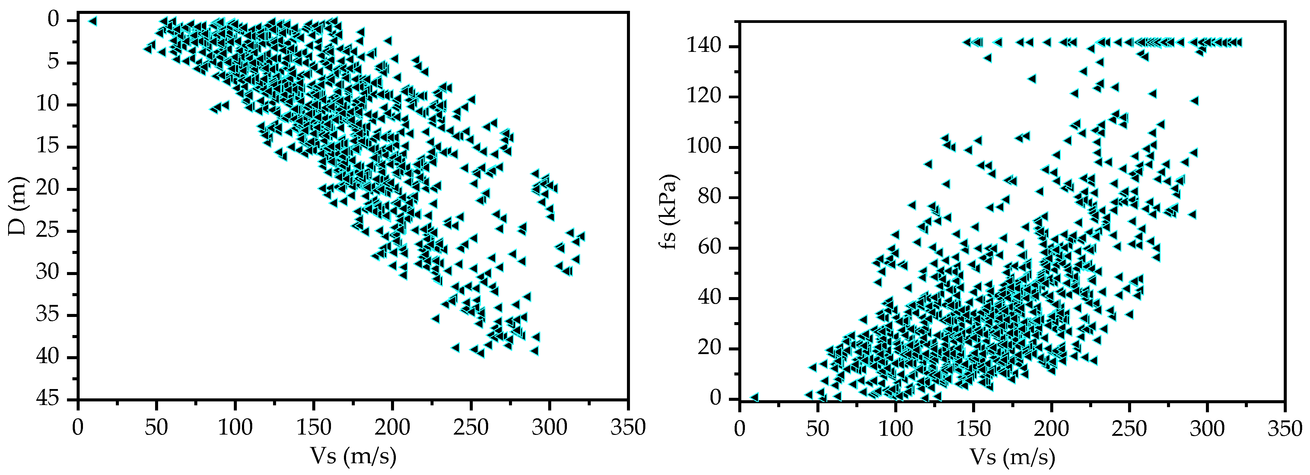
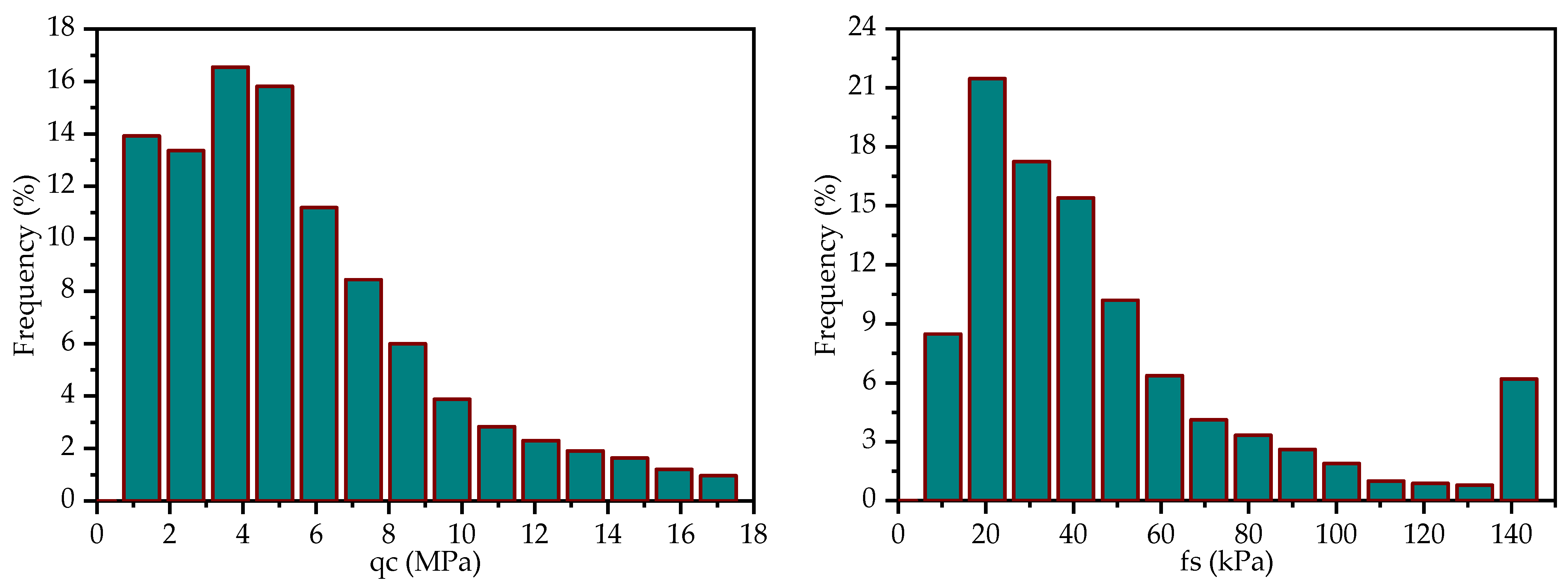
2. Datasets Preprocessing and Visualization

The dataset used in this study was obtained from a previously published dataset [52]. This study utilized 61 CPT soundings, each containing over 1000 q c and f s recordings. These data sets were collected from various regions of Austria, including the Vienna Basin, Gastein Valley, and Zell Basin. The data is publicly accessible and can be downloaded from the following link: https://www.tugraz.at/en/institutes/ibg/research/computational-geotechnics-group/database/ (accessed on 12 May 2023). The CPT datasets were preprocessed before applying ML training and testing techniques. The preprocessing step involved removing outliers from the data. Specifically, outliers were identified and removed from both the q c and f s values in the raw CPT data. Any data point that exceeded twice the interquartile range ( I Q R ) , where I Q R is the difference between the third quartile ( Q 3 ) and the first quartile ( Q 1 ), was considered an outlier. Next, the target variable, which in this case was the shear wave velocity, V s , was estimated using Equation (1) [16]. Subsequently, the datasets were divided into a training set and a testing set, with a ratio of 0.7:0.3 for training and testing purposes.
V S = ( q c σ v 0 p a × 10 0.55 I c + 1.68 )
where q c represents cone tip resistance, σ v 0 represents total overburden pressure, p a represents atmospheric pressure, and   I c represents soil behavioral type index estimated as follows:
I c = ( 3.47 l o g ( ( q c σ v 0 ) / σ v 0 ) 2 + ( l o g F r + 1.22 ) 2 ) 0.5
F r = f s / ( q c σ v 0 ) × 100
where f s represents sleeve friction, σ v 0 is the effective overburden stress, and F r represents normalized friction ratio.
The statistical summaries of both the training and testing datasets considered in this study are presented in Table 1. To gain further insights into the relationship between the input features and the target variable ( V s ), scatter plots are presented in Figure 1. Each scatter plot indicates the correlation between an individual input feature and the target variable. In addition, Figure 2 shows the frequency distribution of the input features and target variable, providing a visual representation of their distribution patterns. Furthermore, box plots of both the input features and the target variable are presented in Figure 3, offering an overview of their distribution.
The interdependencies among input features in ML models can lead to overfitting and decreased efficiency. To assess the correlation between each input feature, a Pearson’s correlation analysis was conducted. Figure 4 displays the correlation coefficients among the input features in the dataset. The correlation coefficients range from −0.08 to 0.51, indicating a combination of weak to moderate correlations among the features. The absence of highly correlated features in the correlation analysis suggests a lower risk of overfitting, as no redundant features were observed.

3. Methodology

This section outlines the training and testing procedures for the ML models used to predict V s . Four ML models, namely RF, SVM, DT and XGBoost, were trained for this purpose. Each ML model was trained on the training datasets, with q c ,   f s , friction ratio ( R f ), and soil depth ( D ) serving as input features and V s as target variable (output). To optimize the performance of these models, the hyperparameters of each model were fine-tuned using a model-based Bayesian optimization technique. To ensure that the models can generalize well to new data, the commonly used k-fold cross-validation techniques were employed. This involves dividing the data into k subsets, training the model on k-1 subsets, and evaluating their performance on the remaining subset. The root mean squared error (RMSE) was used as the evaluation metric to assess the models’ accuracy. In addition to hyperparameter tuning, permutation feature importance and/or recursive feature elimination techniques were applied using the optimized models. This technique was used for the identification and removal of irrelevant features, if present, in the input features. Once the irrelevant features were eliminated, the hyperparameter tuning process was repeated with the updated features to further enhance the models’ performance. Finally, the performances of the optimized models were assessed using the testing dataset. The entire process of training and testing the models is presented in Figure 5, providing a visual representation of the workflow.
The performance of optimized ML models was evaluated using multiple statistical metrics such as root mean squared error (RMSE), mean absolute error (MAE), mean absolute percentage error (MAPE), coefficient of determination ( R 2 ) , scatter index ( S I ), and performance index ( P I ) (see Table 2). Many researchers utilized these indices to evaluate the predictive performance of different ML models [53,54,55,56,57,58,59,60]. The RMSE measures the average magnitude of the errors between the predicted and actual values, indicating the model’s predictive accuracy. A lower RMSE indicates better model performance. MAE estimates the average absolute difference between the predicted and actual values. Like RMSE, a lower MAE indicates better model performance. MAPE represents the average percentage difference between the predicted and actual values. A lower MAPE signifies better model accuracy. R 2 measures the proportion of the variance in the target variable ( V S ) that can be explained by the model, with values closer to 1 indicating a better fit. Furthermore, a newly proposed engineering index ( A 10 I ) was used to evaluate the predictive performance of the models [55,59,61,62,63]. In an ideal model, the value of A 10 I is expected to be one. The A 10 I has significance in engineering as it represents the proportion of samples that fall within ± 10 % deviation from the predicted values compared with the target value. Additionally, the efficiency of the models was evaluated using uncertainty analysis at 95% confidence level ( U 95 ) [64,65].

4. Machine Learning Models

4.1. Random Forests

RF is an ML algorithm that has been widely used for classification and regression tasks [66,67]. It is an ensemble method that combines multiple decision trees to improve predictive accuracy and reduce overfitting. RF has several advantages over other machine learning algorithms, including its ability to handle high-dimensional data, nonlinear relationships between variables, and missing values [68]. In addition, it provides measures of variable importance that can be used for feature selection and interpretation [69].
RF classification and regression can be implemented in R using various packages such as randomForest [68] and ranger [70]. The randomForest package is one of the most widely used packages for RF classification and regression in R. It provides a simple interface for building and evaluating RF models and supports both classification and regression tasks. The ranger package is another popular package for RF classification and regression in R. It is designed to be faster and more memory-efficient than the randomForest package, and supports parallel processing [70].
The ranger package provides several hyperparameters that can be tuned to improve the performance and robustness of RF models. To tune these hyperparameters, one common approach is to use cross-validation. This involves splitting the data into training and test sets, fitting the model on the training set with different combinations of hyperparameters, and evaluating the performance on the validation set. Bayesian optimization is one of the most efficient methods for hyperparameter tuning. It uses a probabilistic model to predict the performance of different hyperparameter configurations based on previous evaluations [71].

4.2. Support Vector Machine

SVMs have gained immense popularity in the field of machine learning due to their ability to solve both classification and regression problems effectively. SVMs work by constructing hyperplanes that can optimally separate data points belonging to different classes or predict target variables with maximum margin. One of the most significant advantages of using SVMs is their ability in handling high-dimensional datasets and nonlinear relationships between variables [72].
In R, e1071 package [73] is commonly utilized to implement SVM models for regression and classification tasks. The package provides options for tuning hyperparameters such as the kernel function, regularization parameter, and cost parameter. One important consideration when using SVMs is their robustness to outliers and noise in the data. Outliers influence the position of the hyperplane and lead to poor generalization performance. To address this issue, Bayesian optimization can be utilized to increase the model’s performance and robustness. Bayesian optimization has been shown to be effective at tuning hyperparameters in various machine-learning algorithms, including SVMs [71].

4.3. Decision Trees

The DT algorithm is commonly used for both classification and regression tasks. The DT algorithms recursively partition data into subsets based on the values of input features and then assign labels to each subset based on the majority class or average value of the target variable. The resulting tree structure can be used to make predictions on new data by traversing the tree from the root node to a leaf node that corresponds to a specific class or value. According to Quinlan [74], decision trees are particularly useful for problems with discrete-valued output variables and can handle both categorical and continuous input features. They are also easy to interpret and visualize, making them a popular choice for exploratory data analysis and decision-making tasks. Figure 6 presents a sample decision tree structure to provide insights into the relationships and decision-making process within the data, aiding in understanding and interpreting the model’s predictions. The node numbers are depicted within the boxes, while the input features are represented by the variables (see Section 1 and Section 3). The green leaves in the figure represent the target value, V s .
The implementation of the DT algorithm for regression tasks is usually performed using the rpart package [75]. The package provides ranges of DT hyperparameters, including complexity parameters, maximum number of trees, minimum number of splits, etc., that can be tuned through grid search or Bayesian optimization. DT algorithms have been used for a variety of geotechnical applicatons, including classification [76,77] and soil parameters predictions.

4.4. eXtreme Gradient Boosting

Recently, the XGBoost algorithm has gained popularity due to its high accuracy and efficiency. XGBoost is an ensemble method that combines multiple weak learners such as decision trees into a single strong learner [78,79]. The algorithm iteratively adds decision trees to the model, with each tree attempting to correct the errors of the previous trees.
XGBoost package [78] is usually utilized to implement the XGBoost regression model in R. The XGBoost package also offers support for hyperparameter tuning, which can significantly improve the model’s performance. It provides a range of options for tuning its hyperparameters, including learning rate (eta), maximum depth of each tree (max_depth), number of trees, and regularization parameters (alpha and gamma). Bayesian optimization can be used for hyperparameter tuning in XGBoost.

5. Results and Discussion

In Section 2, we indicated that the datasets were randomly split into training and testing datasets. The training datasets were used to train the ML models, while the testing datasets were used to evaluate the efficiency of each model in predicting V s . In this section, we will discuss the results obtained from training and testing ML models. All the ML models were trained and tested using a personal computer with 8GB RAM and Intel(R) Core(TM) i7-1065G7 CPU @ 1.30GHz 1.50 GHz processor (Intel Co., Santa Clara, CA, USA). The performance of each ML model was evaluated using the multiple performance metrics listed in Table 2.

5.1. Hyperparameter Optimization Results

The hyperparameters of each model were fine-tuned using Bayesian optimization with a k-fold cross-validation strategy. Specifically, we used 10-fold cross-validation with the RMSE as the evaluation metric for fine-tuning the hyperparameters. The goal was to minimize the RMSE, as lower values indicate better performance. The maximum number of iterations for the fine-tuning process was set to 100 for each model. Figure 7 illustrates the convergence behaviors of the ML models during the fine-tuning process. It shows how the performance metric (RMSE) changed over the iterations. We observed that all the ML models reached stable results within 100 iterations.
Table 3 presents the hyperparameters of the ML models along with their optimized values. The optimized values represent the set of hyperparameters that yielded the best average performance according to the RMSE metric.

5.2. Performance of ML Models

Figure 8 illustrates actual V s and predicted V s using the optimized ML models, along with ± 10 % error lines (red lines). The green lines show a match between actual and predicted V s values. The results demonstrate that all ML models, except for the DT model, achieved excellent predictive accuracy on both training and testing datasets with high R 2 and A 10 I score values of 1. This shows that the RF, SVM, and XGBoost models can explain all the variance in the V s using the given features. Furthermore, the scatter plots for these models show that many data points are closer to the error bounds, indicating that the models performed well. In contrast, the DT model achieved lower R 2 and A 10 I values ranging from 0.94 to 0.95 and from 0.77 to 0.78 on the testing and training data, respectively.
The residual plots of ML models are shown in Figure 9, illustrating a random distribution of points around the horizontal orange line at y = 0 (line of zero error). This indicates that the model’s predictions are unbiased and have captured the underlying patterns in the data. Additionally, the frequency distributions of residuals (green bars) are shown in the figure. The distribution is approximately symmetric, indicating that the errors are normally distributed, a desirable property. To gain more insight into the performance of the ML models, a further comparison is carried out in the following subsection.

5.3. Comparisons of ML Models

Table 4 provides a summary of the evaluation results for the ML models. Based on our results, the DT model exhibited lower accuracy, as evidenced by a lower R 2 on both training and testing data. The DT model recorded RMSE of 13.06 and 13.16, MAE of 10.27 m/s and 10.34 m/s, MAPE of 7.27% and 7.31%, and R 2 of 0.95 and 0.94 on the training and testing datasets, respectively. Additionally, Spider charts were utilized to visualize and assess each model’s efficiency relative to others (Figure 10). The spider chart shows that the DT model significantly diverged towards higher RMSE, MAPE, and MAE on both training and testing datasets in comparison to other ML models. The RF, SVM, and XGBoost models outperform the DT model in terms of RMSE, MAE, MAPE, and R 2 . All RF, SVM, and XGBoost models have lower error values and higher R 2 scores, indicating higher accuracy and better performance in predicting V S from the input features.
Figure 11 illustrates the performance of ML models in predicting V s   as evaluated using four performance metrics: U 95   ,   A 10 I ,   P I ,   and   S I . The results indicate that the DT model achieved lower performance in comparison to other models, as evidenced by its higher U 95   ,   P I ,   and   S I scores and lower A 10 I values. On the other hand, the RF model demonstrated exceptional performance, outperforming the other models in terms of these performance indicators. In terms of S I , the RF, SVM, and XGBoost models achieved excellent precision (EP), with S I < 0.05 on both the training and testing datasets. In contrast, the DT model achieved good precision with 0.05 < S I < 0.1 on the training and testing datasets. Overall, the RF model ranked first, outperforming the other three ML models, while the DT model ranked fourth. The SVM and XGBoost models ranked second and third, respectively.
To further assess the performance of the ML models, a comparison was made between model-predicted V S values and estimated V S values based on existing empirical correlation. A correlation model was selected to estimate V S from CPT soundings. Equation (12) [80] was utilized for the estimation of V S from CPT soundings.
V S = 10 0.31 I c + 0.77 × ( q c σ v 0 ) / p a
where V S is soil shear wave velocity, I c is soil behavior type index, q c is cone tip resistance, σ v 0 is total overburden pressure, and p a is atmospheric pressure.
This correlation model served as a benchmark for evaluating the accuracy and reliability of the ML models’ predictions. Figure 12 illustrates the models’ predictions (red) alongside the profiles of estimated V S values (black) based on the empirical correlations. The results of this comparison indicate a high level of agreement between the predicted V S values and the estimated V S values. This demonstrates that the ML models can produce accurate predictions in line with the established correlations.

6. Conclusions

This study utilized various ML algorithms, including RF, SVM, DT, and XGBoost, to predict V S from CPT data. To train and test these ML models, we used a previously published open-source CPT dataset. The hyperparameters of each ML model were fine-tuned through Bayesian optimization with cross-validation techniques. Eight performance metrics, namely   R M S E ,   M A E ,   M A P E ,   R 2 ,   A 10 I ,   S I ,   P I   and   U 95 , provided quantitative evaluation of the models. Based on our results, the following conclusion can be drawn:
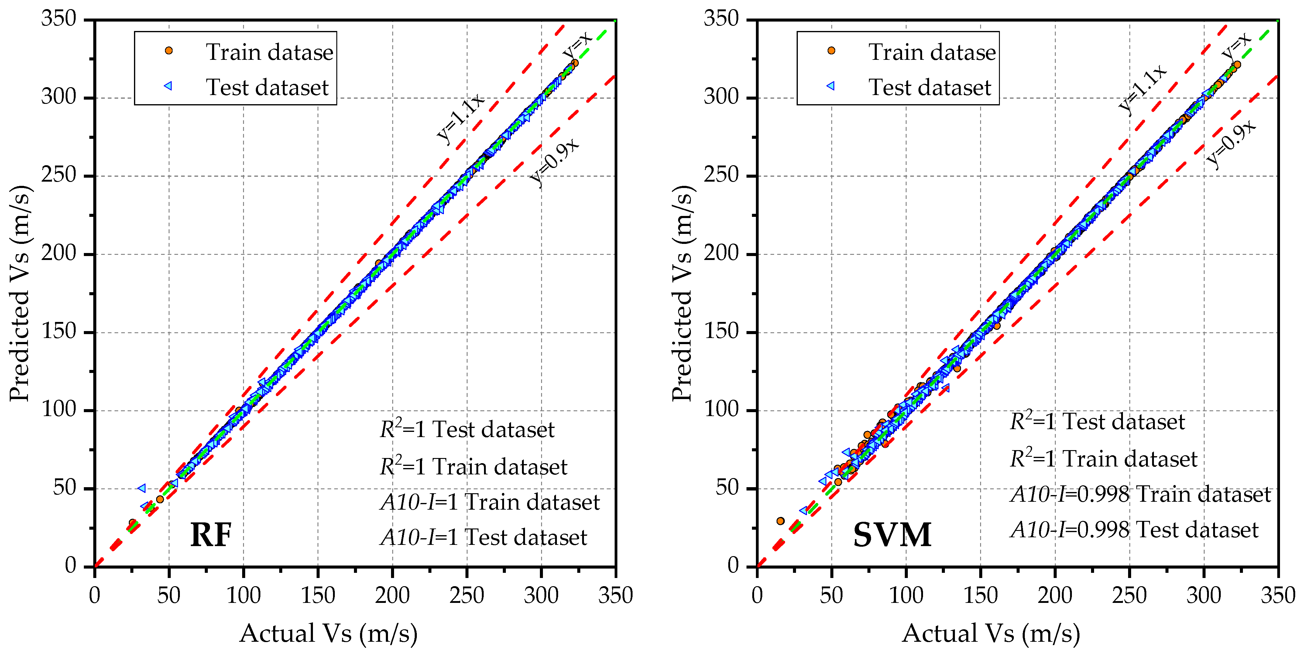
  • The RF model outperformed the other ML models, achieving the lowest error metrics on both the training and testing datasets. Specifically, it achieved an R M S E of 0.46 and 0.96, an M A E of 0.24 m/s and 0.5 m/s, and an M A P E of 0.17% and 0.36%, respectively. The model also demonstrated low scatter, with S I values of 0.003 and 0.006, and P I values of 0.002 and 0.004 on the training and testing datasets, respectively. Additionally, the RF model achieved R 2 and A 10 I values of 1 on both datasets, indicating a perfect fit. Furthermore, the RF model recorded the lowest uncertainty, with a U 95 value of 1.24 on the training dataset.
  • The SVM and XGBoost models also exhibited strong performance, with slightly higher error metrics compared with the RF model. These two models ranked second and third, respectively, following the RF model, which achieved the highest performance. However, the DT model performed poorly, with higher error rates and uncertainty in predicting V s .
  • The RF model demonstrated its overall superior performance and high accuracy in predicting soil V s , even when trained with minimal input features. Hence, owing to its excellent performance across multiple metrics, the RF model can be integrated into a software package for rapid and accurate prediction of soil V s .
  • In summary, while this study relied solely on CPT data for training ML models, it is important to recognize the limitations of the CPT, particularly its primary suitability for fine-grained soils. To further enhance the application of ML models in soil characterization, future research should consider incorporating experimental results and data for coarse-grained soil types.

Author Contributions

Conceptualization, A.T.C. and R.P.R.; methodology, A.T.C.; software, A.T.C.; validation, A.T.C. formal analysis, A.T.C.; writing—original draft preparation, A.T.C.; writing—review and editing, R.P.R.; visualization, A.T.C.; supervision, R.P.R. All authors have read and agreed to the published version of the manuscript.

Funding

This publication was financially supported by Széchenyi István University.

Institutional Review Board Statement

Not applicable.

Informed Consent Statement

Not applicable.

Data Availability Statement

The CPT data can be downloaded from the following link: https://www.tugraz.at/en/institutes/ibg/research/computational-geotechnics-group/database/ (accessed on 12 May 2023).

Conflicts of Interest

The authors declare no conflict of interest.

Abbreviations

A 10 I Engineering index with ± 10 % deviation R 2 Coefficient of determination
A N N Artificial neural network R f Friction ratio
C P T Cone penetration test R F Random forest
D Depth of soil (m) R M S E Root mean squared error
DT Decision trees S C P T Seismic cone penetration testing
F r Normalized friction ratioSDStandard deviation
f s sleeve friction S I Scatter index
I c Soil behavioral type index S V M Support vector machine
I Q R interquartile range U 95 Uncertainty at 95% confidence interval
M A E Mean absolute error V s Shear wave velocity
M A P E Mean absolute percentage error σ v 0 Total overburden stress
M A S W Multi-Channel Analysis of Surface Waves σ v 0 Effective overburden stress
M L Machine learning P a Atmospheric pressure
n Total number of datasets Q 3 Third quartile
P a Atmospheric pressure X ¯ Mean
P I Performance index X i Predicted value of ith observation
q c cone tip resistance X i Actual value of ith observation
Q 1 First quartile X G B o o s t Extreme gradient boosting

References

  1. Kalinina, A.V.; Ammosov, S.M.; Bykova, V.V.; Tatevossian, R.E. Effect of the Upper Part of the Soil Profile on the Site Response. Seism. Instrum. 2018, 54, 499–513. [Google Scholar] [CrossRef]
  2. Kawase, H. Site Effects on Strong Ground Motions. In International Geophysics; Kyushu University: Fukuoka, Japan, 2003; Volume 81, pp. 1013–1030. [Google Scholar]
  3. Borcherdt, R.D.; Glassmoyer, G. On the Characteristics of Local Geology and Their Influence on Ground Motions Generated by the Loma Prieta Earthquake in the San Franciso Bay Region, California. Bull. Seismol. Soc. Am. 1992, 82, 603–641. [Google Scholar] [CrossRef]
  4. Hanks, T.C.; Krawinkler, H. The 1989 Loma Prieta Earthquake and Its Effects: Introduction to the Special Issue. Bull. Seismol. Soc. Am. 1991, 81, 1415–1423. [Google Scholar] [CrossRef]
  5. Aki, K. Local Site Effect on Ground Motion. Am. Soc. Civil Eng. 1988, 20, 103–155. [Google Scholar]
  6. Tokimatsu, K. Geotechnical Site Characterization Using Surface Waves. In Earthquake Geotechnical Engineering, Proceedings of the IS-Tokyo’95, the First International Conference on Earthquake Geotechnical Engineering, Tokyo, Japan, 14–16 November 1995; A.A. Balkema: Rotterdam, The Netherlands, 1995; pp. 1136–1333. [Google Scholar]
  7. Robertson, P.K.; Campanella, R.G. Interpretation of CPT-Sand&Clay. Can. Geotech. J. 1983, 20, 718–733. [Google Scholar]
  8. Park, C.B.; Miller, R.D.; Xia, J. Multichannel Analysis of Surface Waves. Geophysics 1999, 64, 800–808. [Google Scholar] [CrossRef] [Green Version]
  9. Aka, M.; Agbasi, O. Delineation of Weathered Layer Using Uphole and Surface Seismic Refraction Methods in Parts of Niger Delta, Nigeria: Delineation of Weathered Layer. Sultan Qaboos Univ. J. Sci. SQUJS 2021, 26, 58–66. [Google Scholar] [CrossRef]
  10. Musgrave, A.W. Seismic Refraction Prospecting; Society of Exploration Geophysicists: Houston, TX, USA, 1967; ISBN 1560802677. [Google Scholar]
  11. Viggiani, G.; Atkinson, J.H. Interpretation of Bender Element Tests. Geotechnique 1995, 45, 149–154. [Google Scholar] [CrossRef] [Green Version]
  12. Nishio, S.; Tamaoki, K. Measurement of Shear Wave Velocities in Diluvial Gravel Samples Under Triaxial Conditions. Soils Found. 1988, 28, 35–48. [Google Scholar] [CrossRef] [Green Version]
  13. Drnevich, V. Resonant-Column Testing—Problems and Solutions; ASTM International: Singapore, 1978. [Google Scholar]
  14. Le, T.T.; Skentou, A.D.; Mamou, A.; Asteris, P.G. Correlating the Unconfined Compressive Strength of Rock with the Compressional Wave Velocity Effective Porosity and Schmidt Hammer Rebound Number Using Artificial Neural Networks; Springer: Vienna, Austria, 2022; Volume 55, ISBN 0123456789. [Google Scholar]
  15. Andrus, R.D.; Mohanan, N.P.; Piratheepan, P.; Ellis, B.S.; Holzer, T.L. Predicting Shear-Wave Velocity From Cone Penetration Resistance. In Proceedings of the 4th International Conference on Earthquake Geotechnical Engineering, Thessaloniki, Greece, 25–28 June 2007. [Google Scholar]
  16. Robertson, P.K. Interpretation of Cone Penetration Tests—A Unified Approach. Can. Geotech. J. 2009, 46, 1337–1355. [Google Scholar] [CrossRef] [Green Version]
  17. Wolf, Á.; Ray, R.P. Comparison and Improvement of the Existing Cone Penetration Test Results: Shear Wave Velocity Correlations for Hungarian Soils. Int. J. Environ. Chem. Ecol. Geol. Geophys. Eng. 2017, 11, 338–347. [Google Scholar]
  18. Mayne, P.W.; Rix, G.J. Correlations Between Shear Wave Velocity and Cone Tip Resistance in Natural Clays. Soils Found. 1995, 35, 107–110. [Google Scholar] [CrossRef] [PubMed] [Green Version]
  19. Tonni, L.; Simonini, P. Shear Wave Velocity as Function of Cone Penetration Test Measurements in Sand and Silt Mixtures. Eng. Geol. 2013, 163, 55–67. [Google Scholar] [CrossRef]
  20. Robertson, P.K. Cone Penetration Test (CPT)-Based Soil Behaviour Type (SBT) Classification System—An Update. Can. Geotech. J. 2016, 53, 1910–1927. [Google Scholar] [CrossRef]
  21. Robertson, P.K.; Campanella, R.G.; Gillespie, D.; Greig, J. Use of Piezometer Cone Data. In Use of In Situ Tests in Geotechnical Engineering; ASCE: Reston, VA, USA, 1986; pp. 1263–1280. [Google Scholar]
  22. Chen, J.; Vissinga, M.; Shen, Y.; Hu, S.; Beal, E.; Newlin, J. Machine Learning–Based Digital Integration of Geotechnical and Ultrahigh–Frequency Geophysical Data for Offshore Site Characterizations. J. Geotech. Geoenvironmental Eng. 2021, 147, 04021160. [Google Scholar] [CrossRef]
  23. Olayiwola, T.; Tariq, Z.; Abdulraheem, A.; Mahmoud, M. Evolving Strategies for Shear Wave Velocity Estimation: Smart and Ensemble Modeling Approach. Neural Comput. Appl. 2021, 33, 17147–17159. [Google Scholar] [CrossRef]
  24. Assaf, J.; Molnar, S.; El Naggar, M.H. CPT-Vs Correlations for Post-Glacial Sediments in Metropolitan Vancouver. Soil Dyn. Earthq. Eng. 2023, 165, 107693. [Google Scholar] [CrossRef]
  25. Tsiaousi, D.; Travasarou, T.; Drosos, V.; Ugalde, J.; Chacko, J. Machine Learning Applications for Site Characterization Based on CPT Data. In Proceedings of the Geotechnical Earthquake Engineering and Soil Dynamics V, Austin, TX, USA, 10–13 June 2018; American Society of Civil Engineers: Reston, VA, USA, 2018; pp. 461–472. [Google Scholar]
  26. Taheri, A.; Makarian, E.; Manaman, N.S.; Ju, H.; Kim, T.H.; Geem, Z.W.; Rahimizadeh, K. A Fully-Self-Adaptive Harmony Search GMDH-Type Neural Network Algorithm to Estimate Shear-Wave Velocity in Porous Media. Appl. Sci. 2022, 12, 6339. [Google Scholar] [CrossRef]
  27. Kang, T.H.; Choi, S.W.; Lee, C.; Chang, S.H. Soil Classification by Machine Learning Using a Tunnel Boring Machine’s Operating Parameters. Appl. Sci. 2022, 12, 11480. [Google Scholar] [CrossRef]
  28. Carvalho, L.O.; Ribeiro, D.B. Soil Classification System from Cone Penetration Test Data Applying Distance-Based Machine Learning Algorithms. Soils Rocks 2019, 42, 167–178. [Google Scholar] [CrossRef]
  29. Eyo, E.; Abbey, S. Multiclass Stand-Alone and Ensemble Machine Learning Algorithms Utilised to Classify Soils Based on Their Physico-Chemical Characteristics. J. Rock Mech. Geotech. Eng. 2022, 14, 603–615. [Google Scholar] [CrossRef]
  30. Hikouei, I.S.; Kim, S.S.; Mishra, D.R. Machine-Learning Classification of Soil Bulk Density in Salt Marsh Environments. Sensors 2021, 21, 4408. [Google Scholar] [CrossRef]
  31. Aydın, Y.; Işıkdağ, Ü.; Bekdaş, G.; Nigdeli, S.M.; Geem, Z.W. Use of Machine Learning Techniques in Soil Classification. Sustainability 2023, 15, 2374. [Google Scholar] [CrossRef]
  32. Carvalho, L.O.; Ribeiro, D.B. A Multiple Model Machine Learning Approach for Soil Classification from Cone Penetration Test Data. Soils Rocks 2021, 44, 1–14. [Google Scholar] [CrossRef]
  33. Chala, A.T.; Ray, R. Assessing the Performance of Machine Learning Algorithms for Soil Classification Using Cone Penetration Test Data. Appl. Sci. 2023, 13, 5758. [Google Scholar] [CrossRef]
  34. Akhundi, H.; Ghafoori, M.; Lashkaripour, G. Prediction of Shear Wave Velocity Using Artificial Neural Network Technique, Multiple Regression and Petrophysical Data: A Case Study in Asmari Reservoir (SW Iran). Open J. Geol. 2014, 4, 303–313. [Google Scholar] [CrossRef] [Green Version]
  35. Demir, S.; Sahin, E.K. An Investigation of Feature Selection Methods for Soil Liquefaction Prediction Based on Tree-Based Ensemble Algorithms Using AdaBoost, Gradient Boosting, and XGBoost. Neural Comput. Appl. 2023, 35, 3173–3190. [Google Scholar] [CrossRef]
  36. Demir, S.; Şahin, E.K. Liquefaction Prediction with Robust Machine Learning Algorithms (SVM, RF, and XGBoost) Supported by Genetic Algorithm-Based Feature Selection and Parameter Optimization from the Perspective of Data Processing. Environ. Earth Sci. 2022, 81, 459. [Google Scholar] [CrossRef]
  37. Samui, P.; Sitharam, T.G. Machine Learning Modelling for Predicting Soil Liquefaction Susceptibility. Nat. Hazards Earth Syst. Sci. 2011, 11, 1–9. [Google Scholar] [CrossRef] [Green Version]
  38. Ozsagir, M.; Erden, C.; Bol, E.; Sert, S.; Özocak, A. Machine Learning Approaches for Prediction of Fine-Grained Soils Liquefaction. Comput. Geotech. 2022, 152, 105014. [Google Scholar] [CrossRef]
  39. Alobaidi, M.H.; Meguid, M.A.; Chebana, F. Predicting Seismic-Induced Liquefaction through Ensemble Learning Frameworks. Sci. Rep. 2019, 9, 11786. [Google Scholar] [CrossRef] [PubMed] [Green Version]
  40. Jas, K.; Dodagoudar, G.R. Explainable Machine Learning Model for Liquefaction Potential Assessment of Soils Using XGBoost-SHAP. Soil Dyn. Earthq. Eng. 2023, 165, 107662. [Google Scholar] [CrossRef]
  41. Wang, L.; Wu, C.; Tang, L.; Zhang, W.; Lacasse, S.; Liu, H.; Gao, L. Efficient Reliability Analysis of Earth Dam Slope Stability Using Extreme Gradient Boosting Method. Acta Geotech. 2020, 15, 3135–3150. [Google Scholar] [CrossRef]
  42. Zhang, W.; Zhang, R.; Wu, C.; Goh, A.T.C.; Wang, L. Assessment of Basal Heave Stability for Braced Excavations in Anisotropic Clay Using Extreme Gradient Boosting and Random Forest Regression. Undergr. Space 2022, 7, 233–241. [Google Scholar] [CrossRef]
  43. Bharti, J.P.; Mishra, P.; Moorthy, U.; Sathishkumar, V.E.; Cho, Y.; Samui, P. Slope Stability Analysis Using Rf, Gbm, Cart, Bt and Xgboost. Geotech. Geol. Eng. 2021, 39, 3741–3752. [Google Scholar] [CrossRef]
  44. Samui, P. Slope Stability Analysis: A Support Vector Machine Approach. Environ. Geol. 2008, 56, 255–267. [Google Scholar] [CrossRef]
  45. Xiao, L.; Zhang, Y.; Peng, G. Landslide Susceptibility Assessment Using Integrated Deep Learning Algorithm along the China-Nepal Highway. Sensors 2018, 18, 4436. [Google Scholar] [CrossRef] [PubMed] [Green Version]
  46. Nejad, F.P.; Jaksa, M.B. Load-Settlement Behavior Modeling of Single Piles Using Artificial Neural Networks and CPT Data. Comput. Geotech. 2017, 89, 9–21. [Google Scholar] [CrossRef]
  47. Nejad, F.P.; Jaksa, M.B.; Kakhi, M.; McCabe, B.A. Prediction of Pile Settlement Using Artificial Neural Networks Based on Standard Penetration Test Data. Comput. Geotech. 2009, 36, 1125–1133. [Google Scholar] [CrossRef] [Green Version]
  48. Chen, R.; Zhang, P.; Wu, H.; Wang, Z.; Zhong, Z. Prediction of Shield Tunneling-Induced Ground Settlement Using Machine Learning Techniques. Front. Struct. Civ. Eng. 2019, 13, 1363–1378. [Google Scholar] [CrossRef]
  49. Riyadi, Z.A.; Husen, M.H.; Lubis, L.A.; Ridwan, T.K. The Implementation of TPE-Bayesian Hyperparameter Optimization to Predict Shear Wave Velocity Using Machine Learning: Case Study From X Field in Malay Basin. Pet. Coal 2022, 64, 467–488. [Google Scholar]
  50. Shooshpasha, I.; Kordnaeij, A.; Dikmen, U.; Molaabasi, H.; Amir, I. Shear Wave Velocity by Support Vector Machine Based on Geotechnical Soil Properties. Nat. Hazards Earth Syst. Sci. 2014, 2, 2443–2461. [Google Scholar] [CrossRef]
  51. Bagheripour, P.; Gholami, A.; Asoodeh, M.; Vaezzadeh-Asadi, M. Support Vector Regression Based Determination of Shear Wave Velocity. J. Pet. Sci. Eng. 2015, 125, 95–99. [Google Scholar] [CrossRef]
  52. Oberhollenzer, S.; Premstaller, M.; Marte, R.; Tschuchnigg, F.; Erharter, G.H.; Marcher, T. Cone Penetration Test Dataset Premstaller Geotechnik. Data Brief 2021, 34, 106618. [Google Scholar] [CrossRef] [PubMed]
  53. Esmaeili-Falak, M.; Benemaran, R.S. Ensemble Deep Learning-Based Models to Predict the Resilient Modulus of Modified Base Materials Subjected to Wet-Dry Cycles. Geomech. Eng. 2023, 32, 583–600. [Google Scholar]
  54. Harandizadeh, H.; Armaghani, D.J.; Asteris, P.G.; Gandomi, A.H. TBM Performance Prediction Developing a Hybrid ANFIS-PNN Predictive Model Optimized by Imperialism Competitive Algorithm; Springer: London, UK, 2021; Volume 33, ISBN 0052102106. [Google Scholar]
  55. Hajihassani, M.; Abdullah, S.S.; Asteris, P.G.; Armaghani, D.J. A Gene Expression Programming Model for Predicting Tunnel Convergence. Appl. Sci. 2019, 9, 4650. [Google Scholar] [CrossRef] [Green Version]
  56. Li, Z.; Bejarbaneh, B.Y.; Asteris, P.G.; Koopialipoor, M.; Armaghani, D.J.; Tahir, M.M. A Hybrid GEP and WOA Approach to Estimate the Optimal Penetration Rate of TBM in Granitic Rock Mass. Soft Comput. 2021, 25, 11877–11895. [Google Scholar] [CrossRef]
  57. Abushanab, A.; Wakjira, T.G.; Alnahhal, W. Machine Learning-Based Flexural Capacity Prediction of Corroded RC Beams with an Efficient and User-Friendly Tool. Sustainability 2023, 15, 4824. [Google Scholar] [CrossRef]
  58. Wakjira, T.G.; Ebead, U.; Alam, M.S. Machine Learning-Based Shear Capacity Prediction and Reliability Analysis of Shear-Critical RC Beams Strengthened with Inorganic Composites. Case Stud. Constr. Mater. 2022, 16, e01008. [Google Scholar] [CrossRef]
  59. Ahmed, H.U.; Mohammed, A.S.; Faraj, R.H.; Abdalla, A.A.; Qaidi, S.M.A.; Sor, N.H.; Mohammed, A.A. Innovative Modeling Techniques Including MEP, ANN and FQ to Forecast the Compressive Strength of Geopolymer Concrete Modified with Nanoparticles. Neural Comput. Appl. 2023, 35, 12453–12479. [Google Scholar] [CrossRef]
  60. Skentou, A.D.; Bardhan, A.; Mamou, A.; Lemonis, M.E.; Kumar, G.; Samui, P.; Armaghani, D.J.; Asteris, P.G. Closed-Form Equation for Estimating Unconfined Compressive Strength of Granite from Three Non-Destructive Tests Using Soft Computing Models. Rock Mech. Rock Eng. 2023, 56, 487–514. [Google Scholar] [CrossRef]
  61. Xu, H.; Zhou, J.; Asteris, P.G.; Armaghani, D.J.; Tahir, M.M. Supervised Machine Learning Techniques to the Prediction of Tunnel Boring Machine Penetration Rate. Appl. Sci. 2019, 9, 3715. [Google Scholar] [CrossRef] [Green Version]
  62. Mahmood, W.; Mohammed, A. Performance of ANN and M5P-Tree to Forecast the Compressive Strength of Hand-Mix Cement-Grouted Sands Modified with Polymer Using ASTM and BS Standards and Evaluate the Outcomes Using SI with OBJ Assessments. Neural Comput. Appl. 2022, 34, 15031–15051. [Google Scholar] [CrossRef]
  63. Abdalla, A.; Salih, A. Implementation of Multi-Expression Programming (MEP), Artificial Neural Network (ANN), and M5P-Tree to Forecast the Compression Strength Cement-Based Mortar Modified by Calcium Hydroxide at Different Mix Proportions and Curing Ages. Innov. Infrastruct. Solut. 2022, 7, 1–15. [Google Scholar] [CrossRef]
  64. Shi, X.; Yu, X.; Esmaeili-Falak, M. Improved Arithmetic Optimization Algorithm and Its Application to Carbon Fiber Reinforced Polymer-Steel Bond Strength Estimation. Compos. Struct. 2023, 306, 116599. [Google Scholar] [CrossRef]
  65. Behar, O.; Khellaf, A.; Mohammedi, K. Comparison of Solar Radiation Models and Their Validation under Algerian Climate—The Case of Direct Irradiance. Energy Convers. Manag. 2015, 98, 236–251. [Google Scholar] [CrossRef]
  66. Cutler, D.R.; Edwards, T.C.; Beard, K.H.; Cutler, A.; Hess, K.T.; Gibson, J.; Lawler, J.J. Random Forests for Classification in Ecology. Ecology 2007, 88, 2783–2792. [Google Scholar] [CrossRef] [PubMed]
  67. Breiman, L. Random Forests. Mach. Learn. 2001, 45, 5–32. [Google Scholar] [CrossRef] [Green Version]
  68. Liaw, A.; Wiener, M. Classification and Regression by RandomForest. R News 2002, 2, 18–22. [Google Scholar]
  69. Hastie, T.; Tibshirani, R.; Friedman, J.H.; Friedman, J.H. The Elements of Statistical Learning: Data Mining, Inference, and Prediction; Springer: Berlin/Heidelberg, Germany, 2009; Volume 2. [Google Scholar]
  70. Wright, M.N.; Ziegler, A. Ranger: A Fast Implementation of Random Forests for High Dimensional Data in C++ and R. arXiv 2015, arXiv:1508.04409. [Google Scholar] [CrossRef] [Green Version]
  71. Snoek, J.; Larochelle, H.; Adams, R.P. Practical Bayesian Optimization of Machine Learning Algorithms. arXiv 2012, arXiv:1206.2944. [Google Scholar]
  72. Cortes, C.; Vapnik, V. Support-Vector Networks. Mach. Learn. 1995, 20, 273–297. [Google Scholar] [CrossRef]
  73. Meyer, D.; Dimitriadou, E.; Hornik, K.; Weingessel, A.; Leisch, F. E1071: Misc Functions of the Department of Statistics, Probability Theory Group (Formerly: E1071), TU Wien; R Package Version 1.7-13; R Core Team: Vienna, Austria, 2023. [Google Scholar]
  74. Quinlan, J.R. Induction of Decision Trees; Springer: Berlin/Heidelberg, Germany, 1986; Volume 1. [Google Scholar]
  75. Therneau, T.; Atkinson, B.; Ripley, B.; Ripley, M.B. Rpart: Recursive Partitioning and Regression Trees, R Package version 4.1-10; R Core Team: Vienna, Austria, 2015; pp. 1–9. [Google Scholar]
  76. Song, Y.Y.; Lu, Y. Decision Tree Methods: Applications for Classification and Prediction. Shanghai Arch. Psychiatry 2015, 27, 130–135. [Google Scholar] [CrossRef] [PubMed]
  77. Bhattacharya, B.; Solomatine, D.P. Machine Learning in Soil Classification. Neural Networks 2006, 19, 186–195. [Google Scholar] [CrossRef]
  78. Chen, T.; Guestrin, C. Xgboost: A Scalable Tree Boosting System. In Proceedings of the 22nd ACM SIGKDD International Conference on Knowledge Discovery and Data Mining, San Francisco, CA, USA, 13–17 August 2016; pp. 785–794. [Google Scholar]
  79. Fei, Z.; Liang, S.; Cai, Y.; Shen, Y. Ensemble Machine-Learning-Based Prediction Models for the Compressive Strength of Recycled Powder Mortar. Materials 2023, 16, 583. [Google Scholar] [CrossRef]
  80. Ray, R.P.; Wolf, A.; Kegyes-Brassai, O. Harmonizing Dynamic Property Measurements of Hungarian Soils. In Proceedings of the 6th International Conference on Geotechnical and Geophysical Site Characterization (ISC2020), Budapest, Hungary, 7–11 September 2020. [Google Scholar]
Figure 1. Scatter plots of input features with respect to target variable.
Applsci 13 08286 g001aApplsci 13 08286 g001b
Figure 2. Frequency distribution of input features and the target variable.
Applsci 13 08286 g002aApplsci 13 08286 g002b
Figure 3. Box plot of input features and target variable.
Applsci 13 08286 g003aApplsci 13 08286 g003b
Figure 4. Table of feature correlations.
Applsci 13 08286 g004
Figure 5. Flow diagram illustrating machine learning models used for predicting V S .
Applsci 13 08286 g005
Figure 6. Sample decision tree structure illustrating the splitting criteria for predicting the V S .
Applsci 13 08286 g006
Figure 7. Convergence behavior of ML models.
Applsci 13 08286 g007
Figure 8. Scatter plot illustrating the correlation between actual V S and predicted V S .
Applsci 13 08286 g008aApplsci 13 08286 g008b
Figure 9. Scatter plots and frequency distributions of residuals.
Applsci 13 08286 g009aApplsci 13 08286 g009b
Figure 10. Spider plot showing the performance metrics of the different models.
Applsci 13 08286 g010
Figure 11. Performance of ML models based on of U 95   ,   A 10 I ,   P I ,   and   S I indices.
Applsci 13 08286 g011
Figure 12. Comparison of predicted and estimated V S based on empirical correlation.
Applsci 13 08286 g012
Table 1. Statistical summary of training and testing datasets.
FeaturesUnitClassTraining DatasetTesting Dataset
MeanSDMinMaxCountMeanSDMinMaxCount
D mInput12.428.880.014079,57912.388.780.014034,104
q c MPaInput4.893.600.011779,5794.873.590.011734,104
f s kPaInput42.9135.350.0714279,57942.8835.390.1014234,104
R f %Input1.566.110.00112179,5791.576.280.00108334,104
V s m/sTarget166.7655.8910.0632279,579166.5555.579.9332234,104
Table 2. Performance indices used to evaluate the efficiency of the models.
MetricsBest PerformanceEquationsEquation No.
Root mean squared errorLower value R M S E = i = 1 n ( X i X i ) 2 n (4)
Mean absolute errorLower value M A E = 1 n × | i = 1 n X i X i | (5)
Mean absolute percentage errorLower value M A P E = 1 n × | i = 1 n ( X i X i ) X i | × 100 % (6)
Coefficient of determinationunity R 2 = 1 i = 1 n ( X i X i ) 2 ( X i X ¯ ) 2 (7)
A 10 I unity A 10 I = n 10 n (8)
Scatter indexLower value S I = R M S E X ¯ (9)
Performance indexLower value P I = R M S E X ¯ × R 2 + 1 (10)
Uncertainty at 95% confidence levelLower value U 95 = S D 2 + R M S E 2 (11)
S I [64,65]SI < 0.05: excellent precision (EP), 0.05 < SI < 0.1: good precision (GP), 0.1 < SI < 0.15: fair precision (FP), SI > 0.15: poor precision (PP)
n is total number of datasets, X i is the actual value of the ith observation, X i is the predicted value of the ith observation, and X ¯ is mean of target variable. n 10 is the number of samples with actual/predicted value between 0.90 and 1.10, U 95 is uncertainty with 95% confidence intervals, and S D is standard deviation of residuals (the difference between target V s and predicted V s ).
Table 3. Optimized hyperparameters.
ML ModelsTuned Hyperparameters
NamesRangesOptimized Values
RFNumber of variables, mtry1–43
Minimum node of tree1–302
Maximum depth of tree2–10064
Number of trees in the forest1–3012
SVMPenalty parameter, Cost0.1–10058.75
Kernel coefficient, gamma0.01–109.44
Margin of tolerance, Epsilon0.01–10.026
Kernel typeradialradial
DTComplexity parameter, cp0.001–10.001
Maximum depth of trees1–3020
Minimum number of splits2–205
Minimum number of observations
at terminal node, minbucket
2–206
Maximum number of splits at node, maxcompete1–209
XGBoostLearning rate, eta0.01–10.26
Loss reduction term, gamma0.01–103.79
L2 regularization term, lambda0.01–10.38
L1 regularization term, alpha0.01–10.83
Number of boosting rounds, nrounds1–10084
Maximum depth of trees2–109
Fraction of samples for each tree, subsample0.1–10.79
Table 4. Summary of evaluation results for each ML model using training and testing datasets.
ModelsTrain datasetRank
A10 − IRMSE R 2 PISIMAEMAPEU95
RF1 (1)0.46 (1)1 (1)0.002 (1)0.003 (1)0.24 (1)0.17 (1)1.24 (1)1
SVM0.998 (2)1.11 (2)1 (1)0.005 (2)0.007 (2)0.37 (2)0.28 (2)3.07 (2)2
DT0.78 (3)13.1 (4)0.95 (2)0.06 (4)0.08 (4)10.27 (4)7.23 (4)36.20 (4)4
XGBoost1 (1)1.68 (3)1 (1)0.007 (3)0.01 (3)1.29 (3)0.87 (3)4.65 (3)3
ModelsTest datasetRank
A10 − IRMSE R 2 PISIMAEMAPEU95
RF1 (1)0.96 (1)1 (1)0.004 (1)0.006 (1)0.50 (2)0.36 (2)2.66 (2)1
SVM0.998 (2)1.36 (2)1 (1)0.006 (2)0.008 (2)0.38 (1)0.31 (1)2.3 (1)2
DT0.77 (3)13.2 (4)0.94 (2)0.06 (4)0.08 (4)10.34 (4)7.31 (4)36.48 (4)4
XGBoost1 (1)1.86 (3)1 (1)0.008 (3)0.01 (3)1.40 (3)0.94 (3)5.16 (3)3
Disclaimer/Publisher’s Note: The statements, opinions and data contained in all publications are solely those of the individual author(s) and contributor(s) and not of MDPI and/or the editor(s). MDPI and/or the editor(s) disclaim responsibility for any injury to people or property resulting from any ideas, methods, instructions or products referred to in the content.

