Research on Multi-Objective Optimization Model of Foundation Pit Dewatering Based on NSGA-II Algorithm

Abstract

This study focuses on optimizing the foundation pit dewatering scheme using the foundation pit dewatering theory and the principles of multi-objective optimization. It explores the development of a multi-objective optimization model and efficient solution technology for foundation pit dewatering. This research focuses on the foundation pit dewatering project at the inverted siphon section of Xixiayuan canal head, specifically from pile number XZ0+326 to XZ0+500. It establishes an optimized mathematical model for foundation pit dewatering that incorporates three objectives. Additionally, a dewatering optimization program is developed by utilizing the MATLAB optimization toolbox and the multi-objective optimization algorithm program based on the NSGA-II algorithm (Gamultiobj). The multi-objective optimization mathematical model is solved, and a Pareto-optimal solution set with uniform distribution is obtained. The multi-objective optimization evaluation system based on AHP is constructed from the three aspects of dewatering cost, the impact of settlement on the environment, and the safety and stability of the foundation pit. The optimization scheme of the Pareto-optimal solution set is selected as the decision result to provide multiple feasible schemes for the dewatering construction of foundation pits. The optimization scheme is verified by using the GMS software. The simulation results demonstrate that the optimization scheme fulfills the requirements for water level and settlement control. Moreover, the developed optimization program efficiently solves the multi-objective optimization problem associated with foundation pit dewatering. Lastly, an evaluation system incorporating the NSGA-II algorithm and AHP is developed and utilized in the context of dewatering engineering in order to offer multiple viable optimal dewatering schemes.

1. Introduction

In the construction process of various large-scale projects, the dewatering design of the foundation pit is one of the most important technical and scientific issues. The management objectives of foundation pit dewatering under different working conditions (minimum dewatering cost, minimum land subsidence, maximum drawdown of the foundation pit center water level, etc.), dewatering engineering design (well depth, well diameter, etc.), and geological environment constraints (maximum allowable pumping flow of a single well, allowable value of land subsidence, etc.) should be unified in the optimization model. Taking the strong permeable foundation pit dewatering project in the inverted siphon section of the head of the water diversion project of the Xixiayuan Water Conservancy Project in Henan Province as an example, the multi-objective optimization model of foundation pit dewatering based on the NSGA-II algorithm is established in combination with the multi-objective requirements of groundwater level reduction, settlement deformation control, the groundwater environment, and the economic cost.

In recent years, significant progress has been made in the research and application of optimization algorithms at home and abroad. The genetic algorithm, simulated annealing, the Ant colony algorithm, and particle swarm optimization have made important breakthroughs in theoretical research and practical application [1]. The utilization of optimization algorithms is crucial in enhancing efficiency, reducing costs, and optimizing resource utilization.

Reza introduced a variety of multi-objective optimization algorithms to optimize the power generation efficiency of the hydropower station reservoir [2]. Wang applied the NSGA-II algorithm to power grid optimization planning, established the design model of multi-objective power grid planning, and provided schemes for the trade-off analysis of various objectives. Based on the objective function method [3], Xu optimized and analyzed the dewatering plan for a subway foundation pit with the minimum total water inflow as the objective function and combined with the water level constraints of each control point [4]. Liu applied the genetic algorithm to determine the optimal number of wells for foundation pit dewatering and used a simple and efficient genetic algorithm to control a set of model sets to obtain the overall optimal plan [5]. Yang proposed a NPTSGA algorithm, which combines the genetic algorithm and the tabu search algorithm. The algorithm was used to simulate and optimize the problem of seawater intrusion in coastal areas [6]. Fazli incorporated the crossover operator of the genetic algorithm into the position change phase of the firefly algorithm, and fused the two algorithms to solve the optimization problem [7]. Geng introduced the scatter search algorithm into the computational framework of the particle swarm optimization algorithm, and gave full play to their fast convergence characteristics to study the vehicle scheduling problem with uncertain traffic flow [8]. Li proposed a multi-objective optimization algorithm based on particle swarm optimization, which guided the particle swarm to search more fully, improved the diversity and distribution of its non-inferior solutions, and verified the effectiveness of the particle swarm optimization algorithm by using three multi-objective test functions [9]. Ma systematically summarized the basic principle of the genetic algorithm and introduced the simulated annealing algorithm. The annealing operation was added to the original genetic algorithm, and the algorithm was improved to solve the multi-objective optimization model of subway engineering [10].

Nima proposed a new metaheuristic algorithm, the Crystal structure algorithm, which can effectively handle multi-objective problems [11]. Mohamed helped the metaheuristic algorithm to achieve better results in multi-objective optimization problems based on the marine predators algorithm proposed in recent years, and, compared with other algorithms, achieved remarkable results [12]. Thanh proposed a new Shrimp and Gobi joint search algorithm (SGA) for solving large-scale global optimization problems. This algorithm avoids local optima better than population-based algorithms and has faster convergence speed. Thanh also proposed an improved Grey Wolf optimizer (GWO) algorithm, which improves the speed of the algorithm and can be used to study structural damage identification in high-dimensional problems [13,14]. Matteo proposed that the EPLANopt model developed by the Eurac Research Institute was coupled with the multi-objective evolutionary algorithm of DEAP based on Python, which solved the multi-objective optimization problem of optimizing different energy sources [15]. Zhang proposed an improved particle swarm optimization algorithm to solve the model of multimodal multi-objective problems, and introduced the dynamic neighborhood learning strategy instead of the global learning strategy to enhance the diversity of the population [16]. Srinivas studied the concept of non-dominated sorting called the Goldberg algorithm, while searching for multiple Pareto optimal niche and species formation methods. This method can be extended to higher dimensional and more difficult multi-objective problems [17]. Xu proposed a new multi-objective constraint optimization model, which can normalize the weighted sum of the original objective function and the degree of constraint violation on the basis of minimizing both the objective function and the degree of constraint violation (the degree of violation of each constraint or its sum) [18]. Mirjalili proposed a new multi-objective Grasshopper Optimization algorithm based on the navigation of locust swarms in nature. The algorithm can estimate the Pareto optimal frontier of multi-objective problems by combining the target selection and archiving technology [19]. Wang proposed an effective coevolutionary multi-group garden balm optimization algorithm (CMGBO) to ensure the convergence of Pareto regions with good diversity [20]. Zhang proposed an evolutionary strategy for solving multi-modal and multi-objective optimization problems, mainly studying the strategy of finding solutions with good convergence and distribution in the decision space. This strategy can effectively solve multiple groups of optimal solutions simultaneously [21]. Gaurav introduced a multi-objective Seagull Optimization Algorithm. This algorithm introduced the concept of dynamic archiving and had the characteristics of caching the non-dominated Pareto optimal solution [22]. Muhammad proposed a search-based software engineering solution by using a multi-objective evolutionary algorithm. The results of the algorithm can be tested under the background of different objectives and two quality indicators. The results reveal the influence of the attribute of the feature model, the implementation environment, and the number of objectives on the performance of the algorithm [23]. Guan established a multi-objective water supply optimization model considering cost, reliability, and water quality for the mountain water distribution network (WDN). The NSGA-II algorithm was used to optimize the WDN design model in the complex terrain of the mountain area, which provided valuable information for the decision makers in the complex terrain WDN [24]. Li has developed a proxy-assisted stochastic optimization inversion algorithm called “dam parameter identification”. This algorithm assesses the influence of randomly selected training and testing datasets on the modeling and prediction outcomes of artificial neural networks [25]. Huynh used the dataset collected from the Mekong River test project as an example to train and test a multi-objective dataset by evaluating the results of on-site load tests [26].

Taking the multi-objective optimization model of foundation pit dewatering as the main research objective, this paper carries out research through theoretical research, NSGA-II algorithm design, a multi-objective optimization model MATLAB solving Pareto solution set, and GMS numerical simulation verification, and develops a multi-objective optimization program and quantitative evaluation system based on the Analytic Hierarchy Process. The multi-objective dewatering optimization model solution and numerical simulation verification are carried out for the foundation pit dewatering project of the Xixiayuan canal head inverted siphon section at pile number XZ0+326 to XZ0+500, which provides the dewatering optimization decision scheme for the foundation pit dewatering design and construction.

2. Establishment of Multi-Objective Optimization Model and Evaluation System for Foundation Pit Dewatering

2.1. Establishment of Objective Function, Constraints, and Control Conditions

To construct the optimization model with the objective function method, three basic elements should be determined. The first is the objective function, the second is the constraint condition, and the third is the control condition.

2.1.1. Establishment of Objective Function of Optimization Model

Using the objective function method, three objective functions are constructed, as shown in Equations (1) to (4):

(1)

Minimum total cost of dewatering

The objective function is related to the number of wells and the pumping flow of the wells, and the pumping capacity and the number of pumping wells should be reasonably selected to ensure the lowest engineering cost.

$$J_1=Z_{min}={\alpha }_1{\displaystyle \sum }_{i=1}^w{n}_i+{\alpha }_2{\displaystyle \sum }_{i=1}^w{q}_i i=1,2,\dots ,w$$

(1)

Among them, $J_1$ is the minimum target of the total dewatering cost ($Z_{min}$); $w$ is the total number of pumping wells; $n_i$ is a binary variable, indicating whether the $i$-th well is in operation, with a value of 1 indicating operation and 0 indicating no operation; $q_i$ is the flow of the $i$-th pumping well, m³/d; ${\alpha }_1$ is the construction cost of the pumping well; ${\alpha }_2$ is the cost per unit of pumping capacity; and ${\alpha }_1$ and ${\alpha }_2$ are different coefficients related to local market economic conditions.

(2)

The minimum amount of land subsidence caused by dewatering

Considering the influence of dewatering on the premise of meeting the allowable settlement value, it is required that the settlement of important building settlement control points should be the minimum; that is, the settlement influence coefficient should be the minimum. The settlement influence coefficient before optimization is 1, the optimization model can continuously reduce the amount of land subsidence, and the settlement influence coefficient decreases from 1.

$$J_2={\left[C\right]}_{min}=\frac{{{\displaystyle \sum }}_{g=1}^{n_g} {\left[s\right]}_g}{{{\displaystyle \sum }}_{g=1}^{n_g} {\left[s\right]}_y} g=1,2,\dots ,n_g$$

(2)

Among them, $J_2$ is the goal of minimizing the settlement influence coefficient (${\left[C\right]}_{min}$); $n_g$ is the total number of settlement control points; ${\left[s\right]}_y$ is the total allowable settlement, mm; and ${\left[s\right]}_g$ is the optimized settlement of the $g$-th settlement control point, mm.

(3)

The maximum drawdown of the water level in the center of the foundation pit

When implementing the foundation pit dewatering, it is necessary to reduce the groundwater level as much as possible to ensure the safety of the foundation pit structure, but at the same time, it is necessary to ensure that the hydraulic gradient at the bottom of the pit is within the safe allowable range.

$$H^2-h_j^2=\left(2H-S_j\right)S_j={\displaystyle \sum }_{i=1}^{n_w}\frac{q_i}{\pi K}\ln \frac{R_i}{r_{ji}}j=1,2,\dots ,n_j$$

(3)

$$J_3=H_{max}={\displaystyle \sum }_{j=1}^{n_j}\frac{H-h_j}{n_j} j=1,2,\dots ,n_j$$

(4)

Among them, $H$ is the initial water level value of aquifer, m;$h_j$ is the water level value of the $j$-th water level control point after pumping, m; $S_j$ is the water level drawdown value at control point $j$, m; $n_w$ is the number of pumping wells; $q_i$ is the flow rate of the $i$-th pumping well, m³/d; $n_j$ is the number of water level control points; $R_i$ is the influence radius of the pumping well, m; $r_{ji}$ is the distance from the $i$-th well to the $j$-th water level control point, m; $K$ is the permeability coefficient, m/d; $J_3$ is the maximum target of groundwater drawdown at the center of the foundation pit ($H_{max}$), m.

2.1.2. Determination of Constraints in Optimization Model

The multi-objective optimization model of foundation pit dewatering shall meet the following constraints:

(1)

Groundwater level

To meet the construction requirements for foundation pit dewatering, it is necessary to lower the groundwater level in the pit below its bottom and establish water level control points within the pit. The actual drawdown at these control points must exceed the design drawdown.

$$S_j\le {\displaystyle \sum }_{i=1}^w{S}_{ji} j=1,2,\dots ,n_j$$

(5)

where $S_j$ is the design drawdown value at control point $j$, m; $S_{ji}$ is the drawdown of the $i$-th well to the water level control point at $j$, m; $w$ is the number of pumping wells; and $n_j$ is the number of water level control points.

(2)

Single well pumping capacity

The pumping capacity of the pumping well is related to the well structure and aquifer permeability. It is required that the maximum pumping capacity of the pumping well shall not exceed its allowable maximum pumping capacity:

$$0\le q_i\le q_{max}\left(i\right) i=1,2,\dots ,w$$

(6)

where $q_{max}\left(i\right)$ is the maximum pumping capacity of the $i$-th pumping well, m³/d.

(3)

Number of pumping wells

In the construction process of pumping wells, the number of pumping wells needs to be restricted. The restriction of the number of pumping wells in operation is as follows:

$$\sum n_i\le n_{max}$$

(7)

where $n_i$ is whether the $i$-th well exists. If the $i$-th well exists, then $n_i$= 1; if the contrary is true, then $n_i$ = 0. $n_{max}$ is the maximum number of pumping wells when all pumping wells exist.

(4)

Settlement

In order to ensure the environmental safety around the foundation pit, a settlement control point is set. The ground settlement value at the control point should be less than the allowable settlement at this point:

$${\left[s\right]}_g\le {\left[s\right]}_y$$

(8)

where ${\left[s\right]}_g$ is the settlement at control point g, mm; variable ${\left[s\right]}_g$ is the function of state variable $h_i$ and decision variable $q_i$; among them, $h_i$ is the groundwater level, m; $q_i$ is the pumping capacity of a single well, m³/d; and ${\left[s\right]}_y$ is the allowable settlement, mm.

2.1.3. Determination of Optimal Model Control Conditions

The control conditions are used to determine and control the parameter levels of decision variables and state variables, and the well radius and hydraulic gradient of the pumping well are used as the control conditions.

(1)

Well radius

In order to meet the installation of dewatering equipment, the radius of the pumping well is generally required to be greater than or equal to 0.2 m, as follows:

$$0.2\le r_w\left(i\right)$$

(9)

where $r_{w}i$ is the radius of the $i$-th well, taken as 0.2 m.

(2)

Hydraulic gradient

The water level drawdown at the bottom of the foundation pit is the largest. This is the area with the largest hydraulic gradient. There are potential problems of piping or soil flow. The risk level is the highest, which needs to be considered. In order to consider the safety of foundation pit design, the hydraulic gradient is taken as the control condition:

$$K_s=\frac{i_{cr}}{i_{max}}$$

(10)

$$i_{max}=\frac{\Delta h}{\Delta L}$$

(11)

$$i_{cr}=\frac{G_s-1}{e+1}$$

(12)

where $K_s$ is the safety factor, and the safety factor is usually greater than 1.5~2.5 in the dewatering design; $i_{max}$ is the maximum hydraulic gradient; $i_{cr}$ is the critical hydraulic gradient; $h$ is the difference between the internal and external water head, m; $\Delta L$ is the seepage path, m; $G_s$ is the specific gravity of aquifer soil particles; and $e$ is the void ratio.

2.2. Establishment of Multi-Objective Optimization Evaluation System

There is a large number and wide distribution range of the Pareto optimal solution set of the multi-objective optimization model. Each Pareto solution can meet the requirements of foundation pit dewatering. Therefore, the Analytic Hierarchy Process [27] (AHP) combined with the evaluation scoring method can be used to establish the evaluation system, so as to select the candidate set with high score in the Pareto solution set as the decision basis. The most important step for evaluation and decision making is to determine the weight and scoring standard of the sub-target layer (total dewatering cost, settlement influence coefficient, and safety and stability of the foundation pit structure).

The evaluation system based on the multi-objective optimization model of dewatering is structured into two layers. The first layer, denoted as A, represents the main objective of optimizing the foundation pit dewatering. The second layer, referred to as the sub-target layer, includes three components: total dewatering cost (A1), settlement influence coefficient (A2), and safety and stability of the foundation pit structure (A3).

According to the dewatering optimization experience, combined with the Saaty scale table [28], the weight judgment among sub-target layers is carried out, and the judgment matrix A is constructed. The maximum eigenvalue and corresponding eigenvector of the judgment matrix are calculated according to Equation (13):

$$AW={\lambda }_{max}W$$

(13)

where $W$ is the weight corresponding to the sub-target layer, and ${\lambda }_{max}$ is the maximum eigenvalue of the judgment matrix.

In order to avoid the influence of human subjective factors, it is necessary to carry out the consistency test on the constructed judgment matrix and calculate the consistency index $C.I.$ of the judgment matrix and the consistency ratio $C.R.$ Generally, when $C.R.$ < 0.1, the consistency of the constructed judgment matrix can pass the test.

$$C.I.=\frac{{\lambda }_{max}-n}{n-1}$$

(14)

$$C.R.=\frac{C.I.}{R.I.}$$

(15)

where $n$ is the order of the constructed judgment matrix; $C.I.$ is a consistency index; $C.R.$ is the consistency ratio; and $R.I.$ is the average random consistency index.

Therefore, it is seen from

Table 1. A judgment matrix.

A	A1	A2	A3	W0	W0 Normalization
A1	1	1/3	1/5	0.492	0.109
A2	3	1	1/2	1.39	0.309
A3	5	2	1	2.617	0.582

that the judgment matrix of the total dewatering cost, the settlement influence coefficient, and the safety and stability of the foundation pit structure on the total target A in the sub-target layer is constructed, and the weight and normalized weight corresponding to the sub-target layer are calculated according to Equation (13).

The maximum eigenvalue of the judgment matrix ${\lambda }_{max}$ is 3.004. $C.R.$= 0.002 < 0.1 is calculated by the formula, and the consistency of the matrix can pass the test. From the normalized weights of the three sub-objectives, it can be seen that the decision makers are most interested in the safety and stability of the foundation pit structure, followed by the settlement influence coefficient, and, finally, the total cost of dewatering.

In combination with the actual situation and relevant experience of the project, the total cost of dewatering in the sub-target layer, the settlement influence coefficient, and the safety and stability of the foundation pit structure are evaluated and scored, and the score values are shown in

Table 2. Sub-target layer parameter evaluation score.

Sub-Target Layer	Parameter Range	Scoring Value (0–100)
Total cost of dewatering (Minimum total pumping flow, m3/d)	$<$1.45 $\times$ 105	95
	1.45 $\times$ 105–1.5 $\times$ 105	85
	1.5 $\times$ 105–1.55 $\times$ 105	75
	$>$1.55 $\times$ 105	65
Impact of settlement on environment (Settlement influence coefficient)	$<$0.53	90
	0.53–0.55	80
	0.55–0.57	70
Safety and stability of foundation pit structure (The central water level is lower than the foundation pit bottom plate, m)	$>$1.8	90
	0.6–1.8	80
	0–0.6	70

. Therefore, the solution with the highest score in the Pareto optimal solution set in the multi-objective optimization model is selected as the optimization decision solution.

3. Solution of Multi-Objective Optimization Model

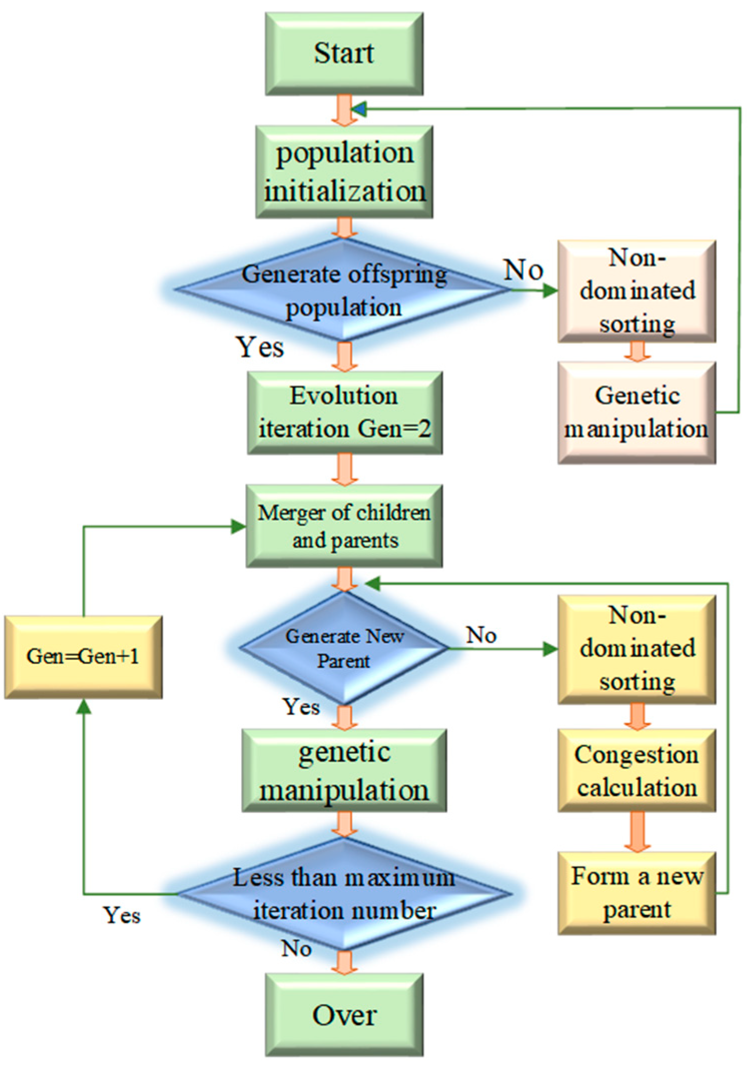
3.1. NSGA-II Algorithm

In 1975, the genetic algorithm appeared in the optimization problem, which was proposed by J Houand and systematically summarized by Goldberg, which realized the development of the population and the continuous improvement of the individual level. The genetic algorithm is based on Darwin’s genetic evolution theory and embodies the idea of “natural selection and survival of the fittest” [29]. The genetic algorithm has the characteristics of self-selection and self-adaptation in evolutionary engineering. It has the ability of global search and it can quickly search all solutions. NSGA-II (non-dominated sorting genetic algorithm) is one of the most widely used and effective multi-objective genetic algorithms [17]. It is an algorithm based on the non-dominated sorting algorithm, which has a small amount of calculation and is an elite algorithm. It was originally proposed for 2–3 objective problems [30]. Compared with the original NSGA algorithm, its computational complexity is greatly reduced, and the computation time is greatly reduced. At the same time, it can ensure the diversity of individuals in the population. Therefore, the NSGA-II algorithm has improved in terms of optimization and computation time compared to the original NSGA algorithm, so it is more excellent as a multi-objective algorithm [31].

The flow chart of the NSGA-II algorithm is shown in Figure 1.

3.2. MATLAB Optimization Toolbox

The MATLAB optimization toolbox is an extension toolbox of the MATLAB software’s numerical calculation. The toolbox has a variety of conventional functions and heuristic algorithms. It has powerful functions, which can be visualized, and it has high solving efficiency [32]. The optimization functions in the optimization toolbox are shown in

Table 3. MATLAB main optimization functions.

Function	Description
Fgoalattain	Multi-objective achievement problem
Fmincon	Constrained nonlinear minimization
Fminimax	Minimization and maximum
Linprog	Linear program
Quadprog	Quadratic programming
Gamultiobj	Multi-objective nonlinear minimization

.

The Gamultiobj program is capable of solving optimization problems with multiple sub-objectives, and it can be utilized either by inputting code or using the graphical toolbox in the MATLAB optimization toolbox. This function incorporates most of the operations from the NSGA-II algorithm, and it is optimized based on it. The Gamultiobj program is consistent with the NSGA-II algorithm in terms of dominance level, non-inferior solution, Pareto ranking, and congestion. However, it introduces the optimal front-end individual coefficient to provide a more precise representation of the Pareto solution. This coefficient has a maximum value of 1 and a minimum value of 0, expressing the ratio of the optimal individual to the total population. A larger ratio results in obtaining more sets of Pareto solutions. The following are the fundamental steps to call the Gamultiobj program, based on the NSGA-II algorithm, for solving practical engineering problems:

(1)

According to the actual engineering conditions in the study area, the expression of the objective function is determined, the decision variables are determined, the constraints and control conditions are established according to the construction requirements, and the optimal mathematical model for solving the problem is established;

(2)

Launch the MATLAB optimization toolbox and utilize the Gamultiobj program to input the established multi-objective optimization mathematical model into the toolbox, following the specific format guidelines;

(3)

Combined with the optimization code, the results of the optimization mathematical model are solved and output.

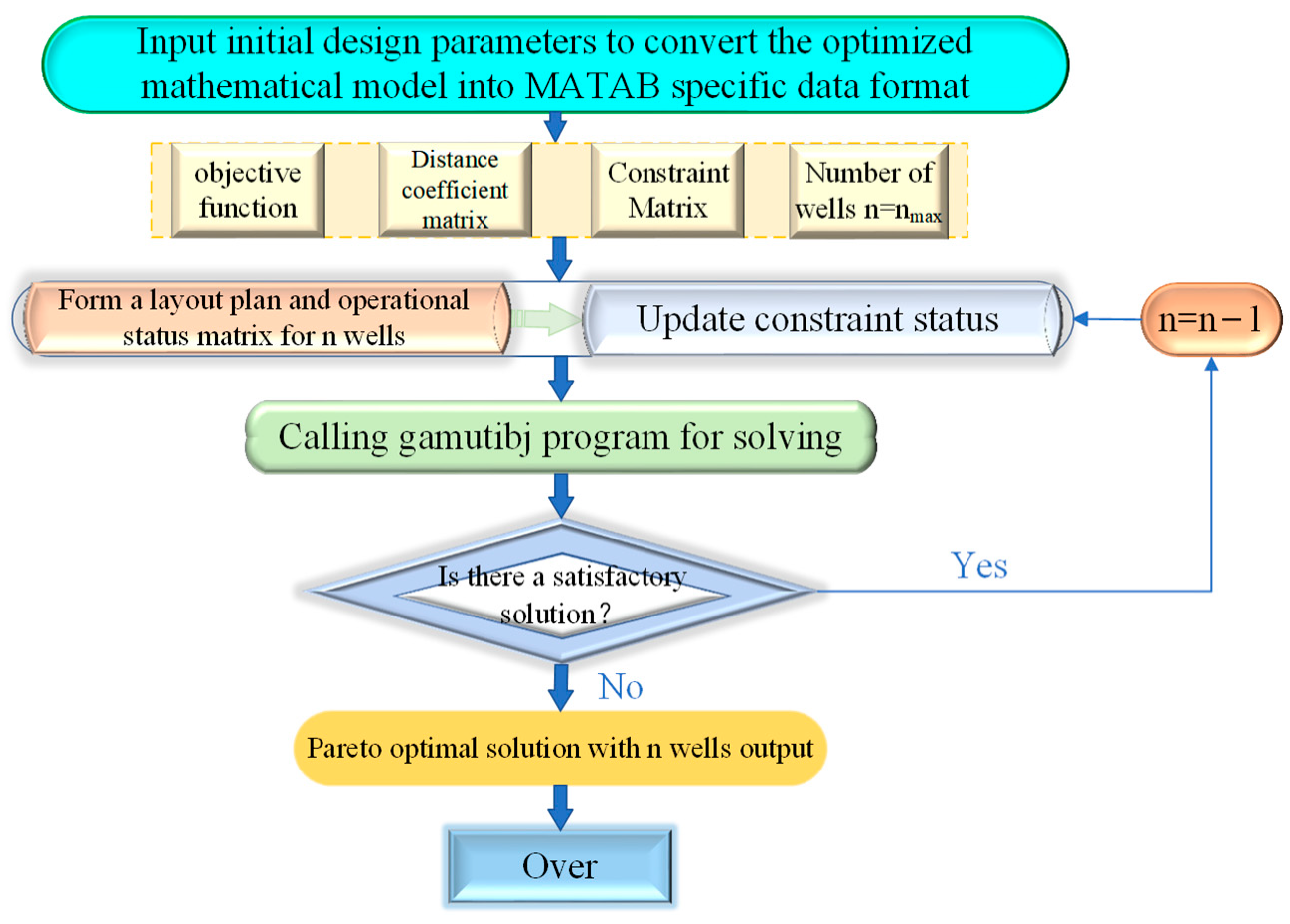
3.3. Program Design for Solving Multi-Objective Optimization Model

The technical route of the optimization solution using the NSGA-II algorithm is shown in Figure 2.

The designed dewatering optimization program has the following advantages:

(1)

The program can simultaneously optimize the number of pumping wells and the pumping capacity of a single well, and it can obtain the Pareto optimal solution set under different working conditions;

(2)

The Pareto solution set is obtained based on the NSGA-II algorithm, with a uniform distribution of Pareto frontiers and while retaining more excellent solutions;

(3)

The program avoids complex programming steps and uses the MATLAB optimization solver to input parameters and output results in a visual form.

4. Engineering Background

4.1. General Situation

The water conservancy and irrigation area engineering of the Xixiayuan water conservancy project is located on the North Bank of the Yellow River in Henan Province, China. It is one of the 172 major water conservancy construction projects in the country. The overview of the study area is shown in Figure 3. This paper focuses on the foundation pit project located at the inverted siphon section of the canal head with the specified pile range (XZ0+326 to XZ0+500). This particular section is situated within the Yellow River wetland protection zone, spanning a total length of 174 meters. Notably, the groundwater is found in a highly permeable pebble layer, approximately 11 meters above the foundation surface. Consequently, the excavation of the foundation pit presents challenges pertaining to dewatering and drainage. The constructed multi-objective optimization model and evaluation system are used to optimize the design of the tube well dewatering scheme, providing a reference for similar projects.

4.1.1. Engineering Geological Conditions

The geomorphic unit of the site belongs to the Yellow River beach area. The terrain is flat and open. It is generally high in the north and low in the south. The ground elevation is 122.19–127.75 m, and the bottom elevation of the foundation pit of the inverted siphon section of the canal head is 111.10–111.30 m.

The stratum is quaternary Holocene alluvium, and the lithology is mainly sandy loam and pebble.

Sandy loam (Q₄^2al) in the first layer: brown yellow, dry or slightly wet, loose, uneven soil, with high sand content in some parts. The thickness is 1.7~2.0 m, and the bottom elevation is 122.02~122.89 m.

Pebble (Q₄^2al) in the second layer: grayish white, purplish red, mixed with a small amount of quartzite and andesite. The particle size is generally 3~6 cm, a small amount of 15~20 cm, and the maximum particle size is more than 20 cm, mostly in sub round shape, accounting for about 55~65%, filled with argillaceous sand and not cemented.

4.1.2. Hydrogeologic Condition

The groundwater in the study area is Quaternary pore phreatic water, which mainly occurs in the pores of the second pebble layer. The buried depth of the groundwater level is 2.60–3.85 m, and the groundwater level is 121.37–121.99 m. Groundwater primarily receives recharge from atmospheric precipitation and the Yellow River, while discharge occurs through evaporation, artificial exploitation, and lateral runoff. The first layer of sandy loam is generally weakly or moderately permeable, with a permeability coefficient of 4 × 10⁻⁴ cm/s. The second layer of pebbles is highly permeable, and the permeability coefficient is generally about 3 × 10⁻¹–1.0 cm/s.

4.2. Initial Scheme of Foundation Pit Dewatering in the Study Area

To achieve dewatering and maintain a dry excavation in the foundation pit of the inverted siphon section of the canal head, this study implements the tube well dewatering method instead of utilizing a waterproof curtain. Moreover, a circular arrangement approach is employed to uniformly position dewatering wells at a distance of 1 m outside the pit to effectively lower the groundwater level. In this paper, the foundation pit with a pile number of XZ0+326–XZ0+500 in the inverted siphon section of the canal head is selected for dewatering design in the pebbles stratum. The length of the foundation pit is 174 meters, and the width is 39 m. The ground elevation of the project area is about 122.5 m, the first layer of sandy loam is about 3 m thick, and the second layer of pebbles is about 20 m thick. The initial groundwater level is about 121.5 m, the bottom elevation of the phreatic aquifer is about 99.5 m, the thickness of the aquifer is about 22 m, the bottom elevation of the foundation pit is 110.3 m, the average excavation depth of the foundation pit is 12 m, the groundwater level is calculated as 1 m below the foundation pit bottom plate, and the drawdown of the water level in the project area is 11~12 m. The engineering geological longitudinal section and foundation pit location of the canal head inverted siphon XZ0+326–XZ0+500 section in the project area is shown in Figure 4. The red line in the figure shows the location of the foundation pit.

The initial design scheme uses a group of phreatic completely penetrating wells for dewatering, which needs to lower the groundwater to 0.5–1 m below the bottom of the foundation pit. According to the technical specification for building a foundation pit (JGJ/120-2012) [33], calculate the total water inflow of the foundation pit:

$$Q=\pi k\frac{\left(2H-s_d\right)s_d}{\ln \left(1+\frac{R}{r_0}\right)}$$

(16)

Among them, $Q$ is the total water inflow, m³/d; $k$ is the permeability coefficient, m/d; $H$ is the thickness of the phreatic aquifer, m; $s_d$ is the design drawdown of the groundwater level of the foundation pit, m; $r_0$ is the equivalent radius of foundation pit, m, which can be calculated according to $r_0=\sqrt{\raisebox{1ex}{$A$}\!\left/ \!\raisebox{-1ex}{$\pi $}\right.}$; $A$ is the area of foundation pit, m²; and $R$ is the influence radius of dewatering, m.

The influence radius of dewatering can be calculated according to the drawdown value of the observation well arranged in the pumping test, combined with the graphical method. If there is no water level observation well, it can also be solved by using the phreatic aquifer empirical formula method with reference to the parameters obtained from the pumping test:

$$R=2s_w\sqrt{kH}$$

(17)

where $s_w$ is the drawdown value of the well water level, m. The meaning of the other symbols is the same as above.

In order to ensure the dewatering effect, the number of tube wells can be calculated using the following formula when tube wells are arranged at equal intervals for dewatering:

$$n=\left(1.1~1.2\right)\frac{Q}{q_{max}}$$

(18)

where $n$ is the number of wells and $q_{max}$ is the maximum water yield of a well, m³/d.

The maximum allowable pumping capacity of the pumping well is generally obtained from the pumping test. In the absence of a pumping test, it can be solved according to the following empirical formula:

$$q_{max}=120\pi rl\sqrt[3]{K}$$

(19)

where $q_{max}\left(i\right)$ is the maximum pumping capacity of the $i$-th pumping well, m³/d; $r$ is the screen radius of the pumping well, m; and $l$ is the effective working length of the screen of the pumping well, m.

According to the construction quality acceptance code for building foundation engineering (GB50202-2018) [34], the allowable settlement value caused by foundation pit dewatering is 15 mm, which is related to the height of the dam.

Then, based on survey data and on-site slug test techniques [35,36,37,38], the permeability coefficient of the aquifer was obtained. The initial design scheme calculation parameters are shown in

Table 4. Calculation parameters of initial design scheme.

Foundation Pit Section	K/(m/d)	Influence Radius R/(m)	${\mathit{q}}_{\mathit{m}\mathit{a}\mathit{x}}$/ (m3/d)	Number of Pumping Wells	Water Level Control Point	Settlement Control Points	Total Q/(m3/d)
XZ0+326– XZ0+500	432	2242.5	6000	26	5	2	156,000

.

According to the calculation parameters of the initial design scheme, 26 phreatic completely penetrating wells are planned to be arranged, 5 water level control points K1–K5 are arranged along the longitudinal axis of the foundation pit, and 2 settlement control points P1 and P2 are arranged next to the dam of the Xixiayuan water conservancy project in the southwest, as shown in Figure 3.

5. Solving Pareto Optimal Solution Set and Analysis Decision

The multi-objective optimization model of foundation pit dewatering based on the NSGA-II algorithm optimizes the preliminary design scheme, inputs the initial design parameters, calls the Gamultiobj program, and sets the parameters. The initial population size of the Gamultiobj program is set to 100, the genetic iteration is set to 30 generations, the cross ratio is set to 0.7, the function tolerance is set to 1 × 10⁻⁶, and the Pareto set ratio is set to 0.6; that is, the Pareto solution set is generated after 3000 operations and 30 iterations of the function. Through the optimization calculation, in order to meet the program convergence, constraints, and control conditions, at least 24 pumping wells need to be operated. Therefore, the Pareto optimal solution set under three working conditions (24–26 pumping wells in operation) is obtained. The constructed dewatering multi-objective optimization evaluation system assigns scores and evaluates the Pareto optimal solution set. Based on the higher evaluation score, the Pareto solution is analyzed to serve as the foundation for decision making. To assess the feasibility of the proposed scheme, a numerical simulation was conducted to verify its feasibility in Section 6.

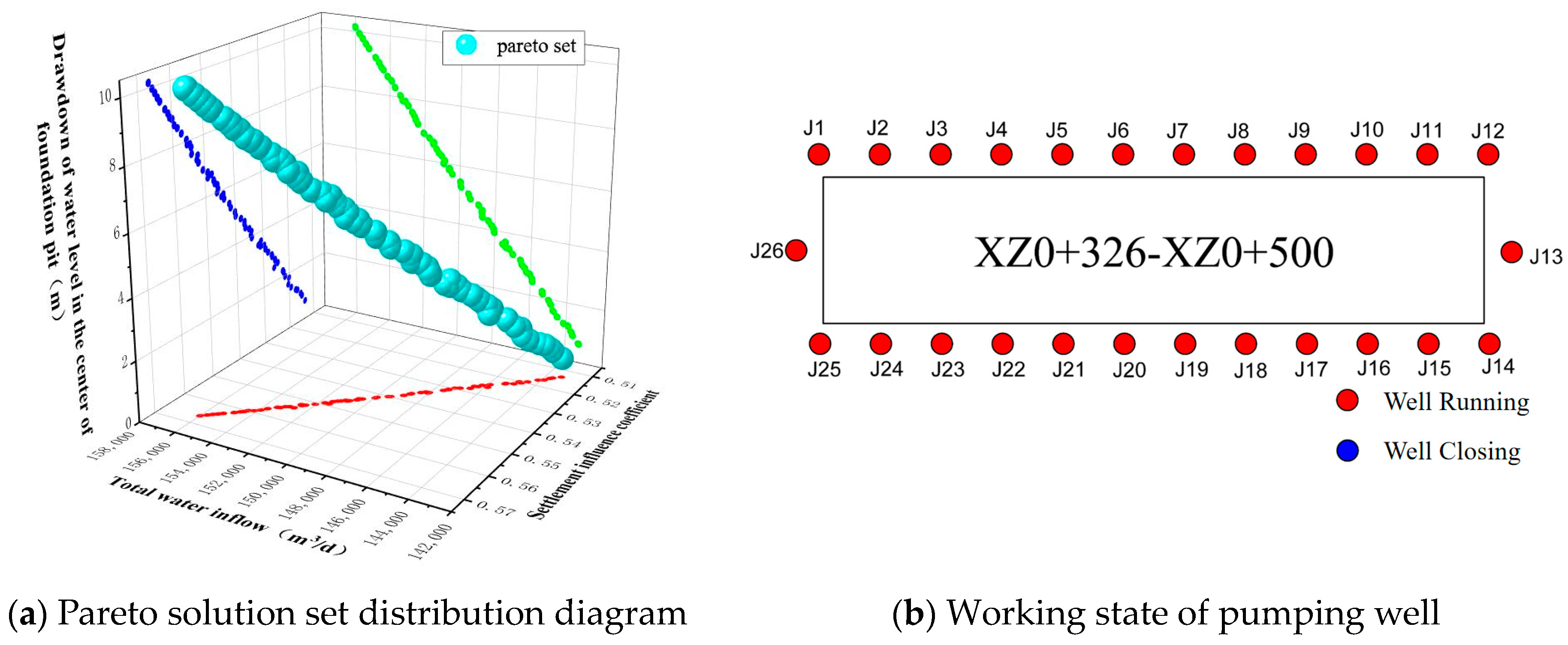
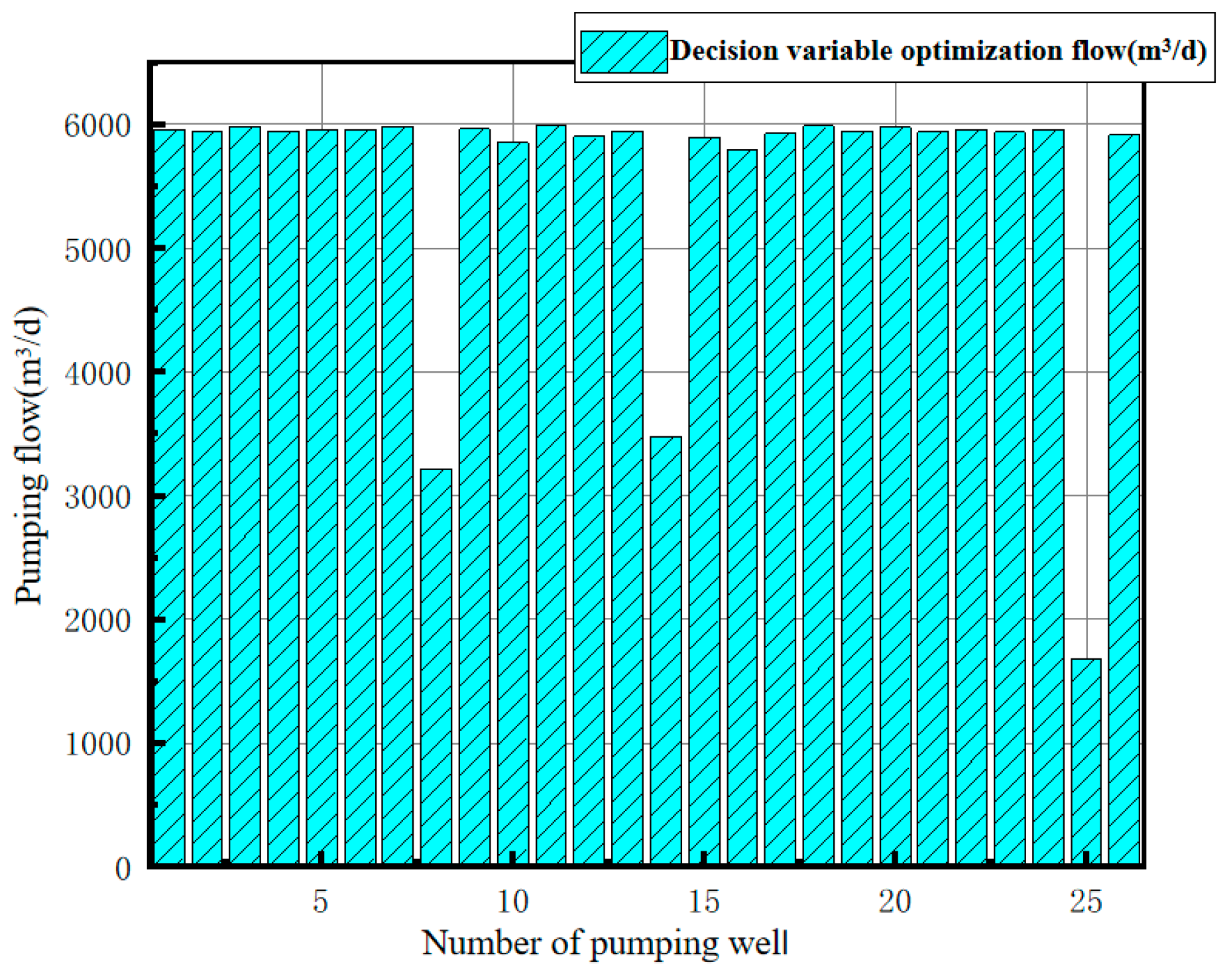
5.1. Pareto Optimal Solution Set and Analysis of Running 26 Pumping Wells Schemes

The multi-objective optimization model for foundation pit dewatering allows for the identification of Pareto optimal solutions and the generation of multiple dewatering schemes tailored to different objectives. The first working condition is set with 26 running wells, and the Gamultiobj program, based on the NSGA-II algorithm, is employed to obtain the Pareto optimal solution set and the operational status of the pumping wells. This information is depicted in Figure 5.

It can be seen from Figure 5 that the optimization model maintains the running of all of the initial 26 pumping wells. After 30 iterations of the algorithm, the Pareto optimal solution set is obtained. The light green color ball in the solution set is the Pareto optimal solution. The red dot indicates the relationship between the total water inflow of the foundation pit and the settlement influence coefficient, the green dot indicates the relationship between the central water level drawdown of the foundation pit and the total water inflow, and the blue dot indicates the relationship between the central water level drawdown of the foundation pit and the settlement influence coefficient. Under the condition of meeting constraints and control conditions, the total water inflow ranges from 1.42 × 10⁵ to 1.56 × 10⁵ m³/d. The settlement influence coefficient is between 0.51 and 0.57, which is converted into the settlement value of 7.65–8.55 mm, which is less than the allowable settlement value of 15 mm. The drawdown of the water level in the center of the foundation pit is 0.2–10 m, meeting the drawdown requirements of more than 0 m. All Pareto solutions of 26 pumping wells under all running conditions are substituted into the dewatering multi-objective optimization evaluation system to calculate the evaluation score, which is arranged in descending order according to the weighted scores of the three objectives. The score results of Pareto solutions obtained by the scheme are shown in

Table 5. Evaluation table for optimal scheme of foundation pit dewatering for running 26 pumping wells.

Pareto Solution No.	Score for Objective Ⅰ	Score for Objective Ⅱ	Score of Objective Ⅲ	Weighted Scores of Three Objectives of Dewatering Optimization
1	95	90	90	90.545
2	85	90	90	89.455
3	85	80	90	86.365
4	75	80	90	85.275
5	95	90	80	84.725
6	75	70	90	82.185
7	65	70	90	81.095

.

It can be seen from Table 5 that the solutions in the Pareto optimal solution set are evaluated by AHP combined with the scoring method, and the Pareto solution with a high evaluation score is selected. So, the dewatering scheme with a weighted evaluation score of 90.545 is selected. The comparison of the optimization results of the three objectives is shown in

Table 6. Three objective optimization results of running 26 pumping wells.

	Each Objective	Well Status	Total Pumping Flow/(m3/d)	Settlement Value (mm)	The Distance Where Water Level in the Center of the Foundation Pit Is Lower than the Bottom Plate/(m)	Hydraulic Gradient Value
Schemes
Preliminary scheme		26 wells in running	156,000	<15	>0	<0.9
The first optimized working condition		26 wells in running	144,972	7.8	1.84	0.65

, and the optimal results of decision variables are shown in Figure 6.

It can be seen from Table 6 that the total water inflow of objective I under the first optimization working condition is about 1.45 × 10⁵ m³/d, the settlement value of objective II is 7.8 mm, which is less than the allowable settlement value of 15 mm, and the foundation pit central water level of objective III is 0.39 m lower than the foundation pit bottom plate, meeting the design requirements for construction of more than 0 m. In this scheme, if the construction and installation of the pumping well have been completed, the score of the three objectives is the best, but the disadvantage is that the number of the pumping wells is the largest, and it is not necessarily the best scheme in the area with a high cost of construction and installation of the pumping well.

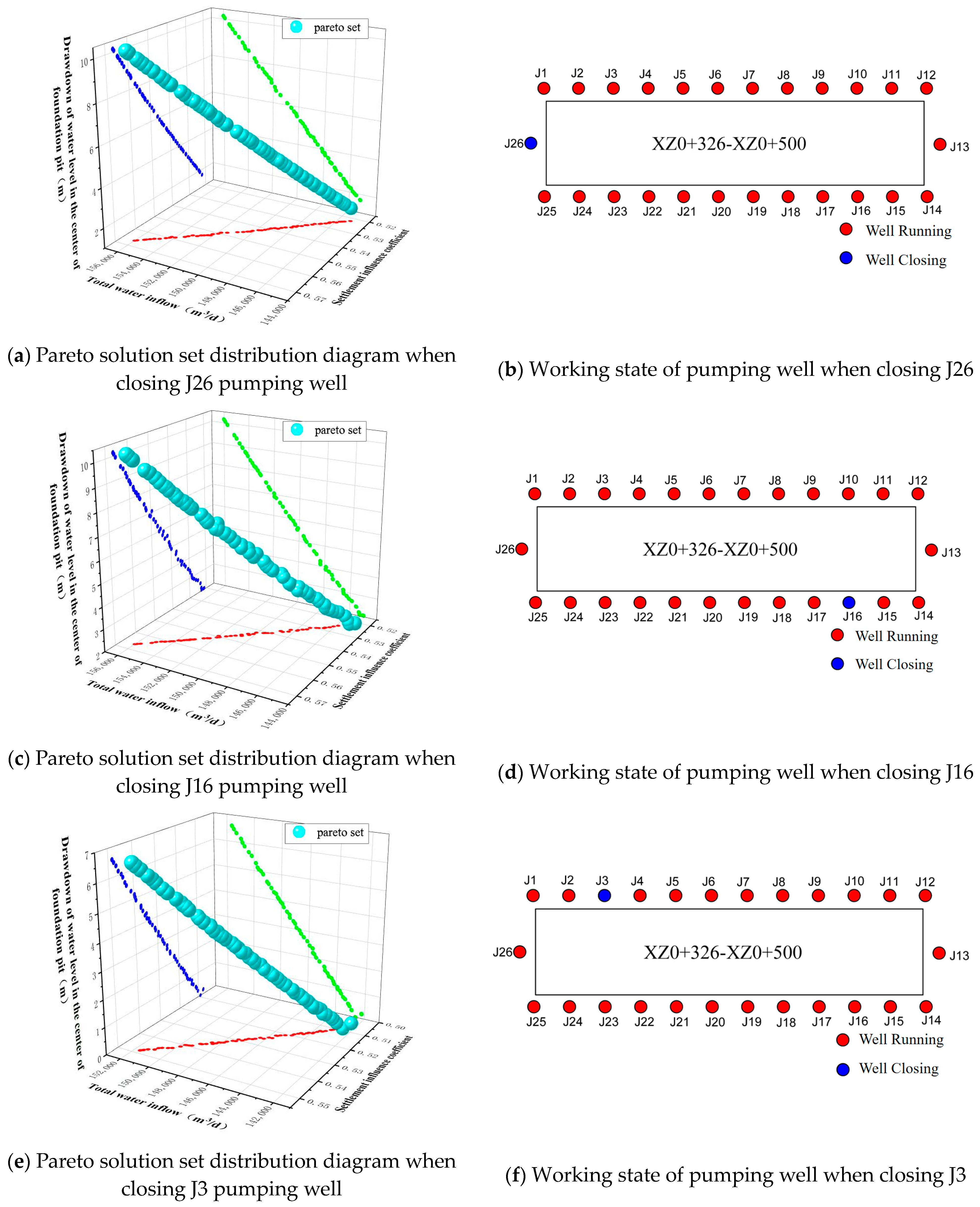
5.2. Pareto Optimal Solution Set and Analysis of Running 25 Pumping Wells Schemes

Similarly, on the premise of meeting the constraints and control conditions, the second optimization working condition is set to arbitrarily close one of the wells, resulting in a total of 26 layout schemes, without changing the location of the wells in the preliminary layout scheme. After optimization by the Gamultiobj program, 26 sets of Pareto solution sets are obtained, and 26 feasible schemes can be optimized for three objectives. Three sets of layout optimization schemes with evenly distributed Pareto solution sets are selected for analysis. The Pareto optimal solution set and pumping well layout state under the second optimization working condition are shown in Figure 7.

It can be seen from Figure 7 that the three schemes under the second optimized working condition are to close the J26, J16, or J3 pumping well, respectively. Similarly, all Pareto solutions of the three schemes under the second optimization condition are substituted into the dewatering multi-objective optimization evaluation system, and the evaluation scores are calculated. The weighted scores of the three objectives are arranged in descending order. The score results of the Pareto solutions of each scheme are shown in

Table 7. Evaluation table for optimal scheme of foundation pit dewatering for running 25 pumping wells.

Each Scheme	Pareto Solution No.	Score for Objective Ⅰ	Score for Objective Ⅱ	Score of Objective Ⅲ	Weighted Scores of Three Objectives of Dewatering Optimization
Close J26 pumping well	1	85	90	90	89.455
	2	85	80	90	86.365
	3	75	80	90	85.275
	4	95	90	80	84.725
	5	85	90	80	83.635
	6	65	70	90	81.095
Close J16 pumping well	1	85	90	90	89.455
	2	85	90	90	89.455
	3	85	80	90	86.365
	4	75	80	90	85.275
	5	95	90	80	84.725
	6	75	70	90	82.185
Close J3 pumping well	1	85	90	90	89.455
	2	85	90	90	89.455
	3	85	80	90	86.365
	4	75	80	90	85.275
	5	95	90	80	84.725
	6	75	70	90	82.185

.

Select the Pareto solution with the highest evaluation score among the dewatering optimization schemes in Table 7, which are the three dewatering schemes with weighted scores of 89.455, 90.545, and 89.455, respectively. The comparison of the optimization results of the three objectives is shown in

Table 8. Three objective optimization results of running 25 pumping wells.

	Each Objective	Well Status	Total Pumping Flow/(m3/d)	Settlement Value (mm)	The Distance Where Water Level in the Center of the Foundation Pit Is Lower than the Bottom Plate/(m)	Hydraulic Gradient Value
Schemes
Preliminary scheme		26 wells in running	156,000	<15	>0	<0.9
The second optimized working condition		Close J26	145,498	7.9	1.85	0.65
		Close J16	149,608	8.4	1.88	0.67
		Close J3	145,037	7.7	1.83	0.63

. The optimal results of decision variables are shown in Figure 8.

It can be seen from Table 8 that the total water inflow of objective I under the second optimized working condition is 1.45 × 10⁵–1.49 × 10⁵ m³/d, and the settlement value of objective II is between 7.85 and 8.4 mm, which is less than the allowable settlement value of 15 mm. The foundation pit central water level of objective III is 1.83–1.88 m lower than the foundation pit bottom plate, which meets the requirements of construction of more than 0 m. In this scheme, the highest evaluation scores for separately closing pumping wells J26, J16, or J3 are basically the same, but according to Table 8, the advantages and disadvantages of each scheme can be analyzed in detail. If the minimum settlement and the lowest hydraulic gradient are considered, pumping well J3 should be shut down; if the maximum water level drawdown value and the safest structure are considered, pumping well J16 should be shut down.

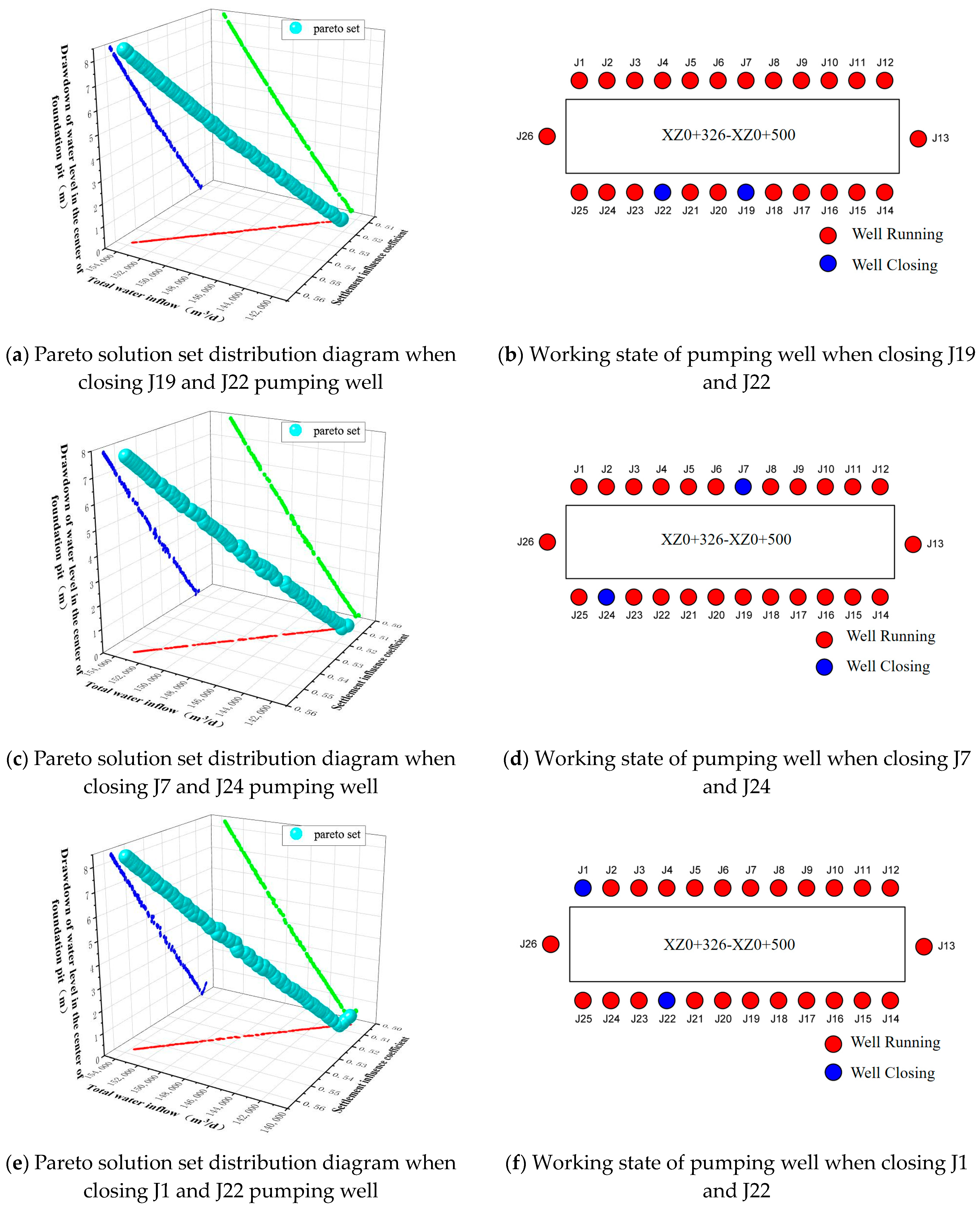
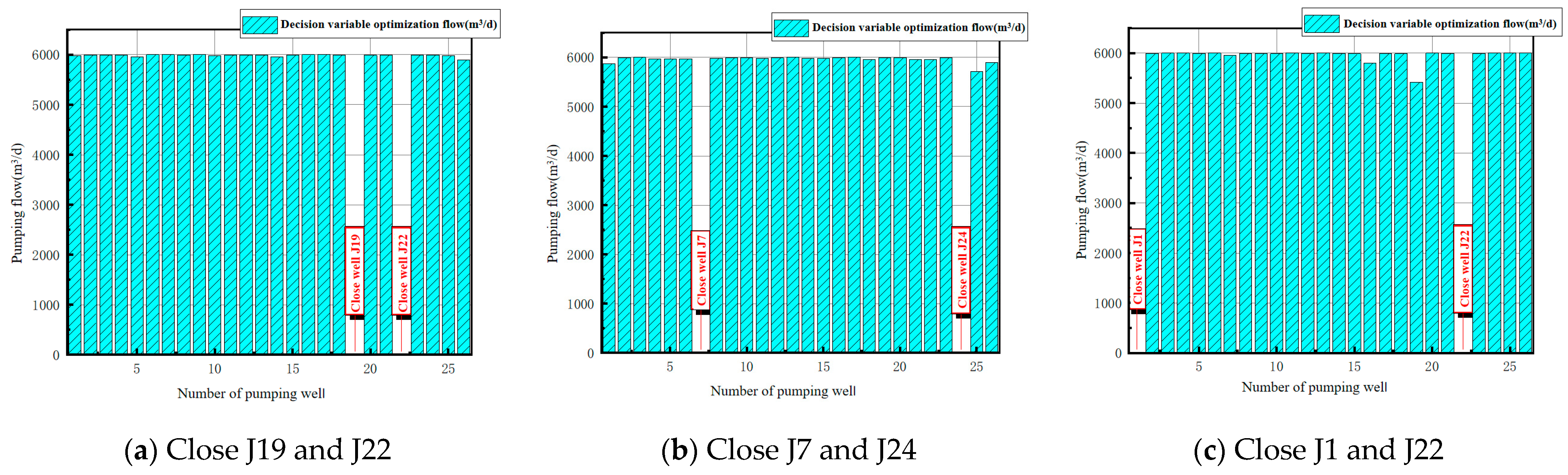
5.3. Pareto Optimal Solution Set and Analysis of Running 24 Pumping Wells Schemes

Similarly, on the premise of meeting the constraints and control conditions, the third optimal working condition is set to arbitrarily close two of the pumping wells, resulting in a total of 325 layout schemes, which does not change the location of the wells in the preliminary layout scheme. After the optimization of the Gamultiobj program, the program converges to 100 sets of Pareto solution sets, and 100 feasible schemes can be optimized for the three objectives. Three sets of layout optimization schemes with evenly distributed Pareto solution sets under the third working condition are selected for analysis. Pareto optimal solution sets and the pumping well layout status are shown in Figure 9.

It can be seen from Figure 9 that under the third optimization condition, the optimization model runs 24 pumping wells. Scheme 1 is to close the J19 and J22 pumping wells, scheme 2 is to close the J7 and J24 pumping wells, and scheme 3 is to close the J1 and J22 pumping wells. Similarly, all Pareto solutions of the three schemes under the third optimization condition are substituted into the dewatering multi-objective optimization evaluation system, and the evaluation scores are calculated. The weighted scores of the three objectives are arranged in descending order from larger to smaller. The score results of Pareto solutions of each scheme are shown in

Table 9. Evaluation table for optimal scheme of foundation pit dewatering for running 24 pumping wells.

Each Scheme	Pareto Solution No.	Score for Objective Ⅰ	Score for Objective Ⅱ	Score of Objective Ⅲ	Weighted Scores of Three Objectives of Dewatering Optimization
Close J19 and J22 pumping wells	1	95	90	90	90.545
	2	85	80	90	86.365
	3	75	80	90	85.275
	4	95	90	80	84.725
	5	75	70	90	82.185
	6	95	90	70	78.905
Close J7 and J24 pumping wells	1	95	90	90	90.545
	2	85	80	90	86.365
	3	75	80	90	85.275
	4	95	90	80	84.725
	5	75	70	90	82.185
	6	95	90	70	78.905
Close J1 and J22 pumping wells	1	95	90	90	90.545
	2	85	80	90	86.365
	3	75	80	90	85.275
	4	95	90	80	84.725
	5	75	70	90	82.185
	6	95	90	70	78.905

.

Select the Pareto solution with the highest evaluation score in the dewatering optimization scheme in Table 9; that is, the three groups of dewatering schemes with the same weighted score of 89.455. The comparison of three objective optimization results is shown in

Table 10. Three objective optimization results of running 24 pumping wells.

	Each Objective	Well Status	Total Water Inflow/(m3/d)	Settlement Value (mm)	The Distance Where Water Level in the Center of the Foundation Pit Is Lower Than the Bottom Plate/(m)	Hydraulic Gradient Value
Schemes
Preliminary scheme		26 wells in running	156,000	<15	>0	<0.9
The third optimized working condition		Close J19, J22	143,665	7.95	1.84	0.66
		Close J7, J24	143,121	7.95	1.83	0.65
		Close J1, J22	143,036	7.95	1.83	0.65

. The optimization results of decision variables are shown in Figure 10.

It can be seen from Table 10 that the total water inflow of objective I under the third optimized condition is about 1.43 × 10⁵ m³/d, the ground settlement value of objective II is about 7.95 mm, which is less than the allowable settlement value of 15 mm, and the foundation pit central water level of objective III is 1.83–1.84 m lower than the foundation pit bottom plate. In this scheme, due to the minimum number of pumping wells and pumping capacity, the cost of dewatering is minimized. However, disadvantages of this scheme are that the settlement of the control point is relatively large, particularly in residential areas where this may not be the optimal choice.

5.4. Pareto Optimal Solution Set Analysis and Decision Making

The multi-objective optimization model of foundation pit dewatering based on the NSGA-II algorithm is solved to obtain the Pareto optimal solution set under three different dewatering conditions. Using the multi-objective optimization evaluation system, the optimization scheme in the Pareto optimal solution set is selected as the decision optimization result from the three objectives of total dewatering cost, settlement influence coefficient, and the safety and stability of the foundation pit structure, which provides a variety of feasible schemes for the dewatering construction of the foundation pit.

The three objectives in the foundation pit dewatering optimization model affect and interact with each other. Therefore, the specific analysis and decision making are as follows:

(1)

When giving priority to the total cost of dewatering, it is important to consider the drilling and pumping costs for foundation pit dewatering. Within the optional Pareto solution set, a solution with a smaller number of pumping wells and lower total pumping capacity should be the first choice based on the dewatering multi-objective optimization evaluation system. Specifically, the operation scheme of closing the J1 and J22 pumping wells under the third optimization condition can be preferred;

(2)

If the focus is on the impact of dewatering on the surrounding environment, preference should be given to a dewatering scheme with a settlement impact coefficient of less than 0.53. Specifically, the operation scheme corresponding to Pareto solution No. 1 under the first optimized condition in Table 5, and the operation scheme corresponding to closing the J3 pumping well under the second optimized condition in Table 7, can ensure minimal ground settlement under the conditions of meeting the total cost requirements of dewatering and the safety and stability of the foundation pit structure;

(3)

When prioritizing the safety and stability of the foundation pit structure, achieving a significant drawdown of the water level in the center of the foundation pit is crucial for ensuring successful construction and enhancing structural safety. Considering the dewatering multi-objective optimization evaluation system, a preferable dewatering scheme is to maintain the water level approximately 1.5 m below the bottom plate of the foundation pit. Therefore, the operation scheme of running 25 pumping wells while closing the J16 pumping well under the second working condition is recommended to meet the maximum drawdown of the water level.

6. Numerical Simulation Verification of Dewatering Optimization Scheme Based on GMS

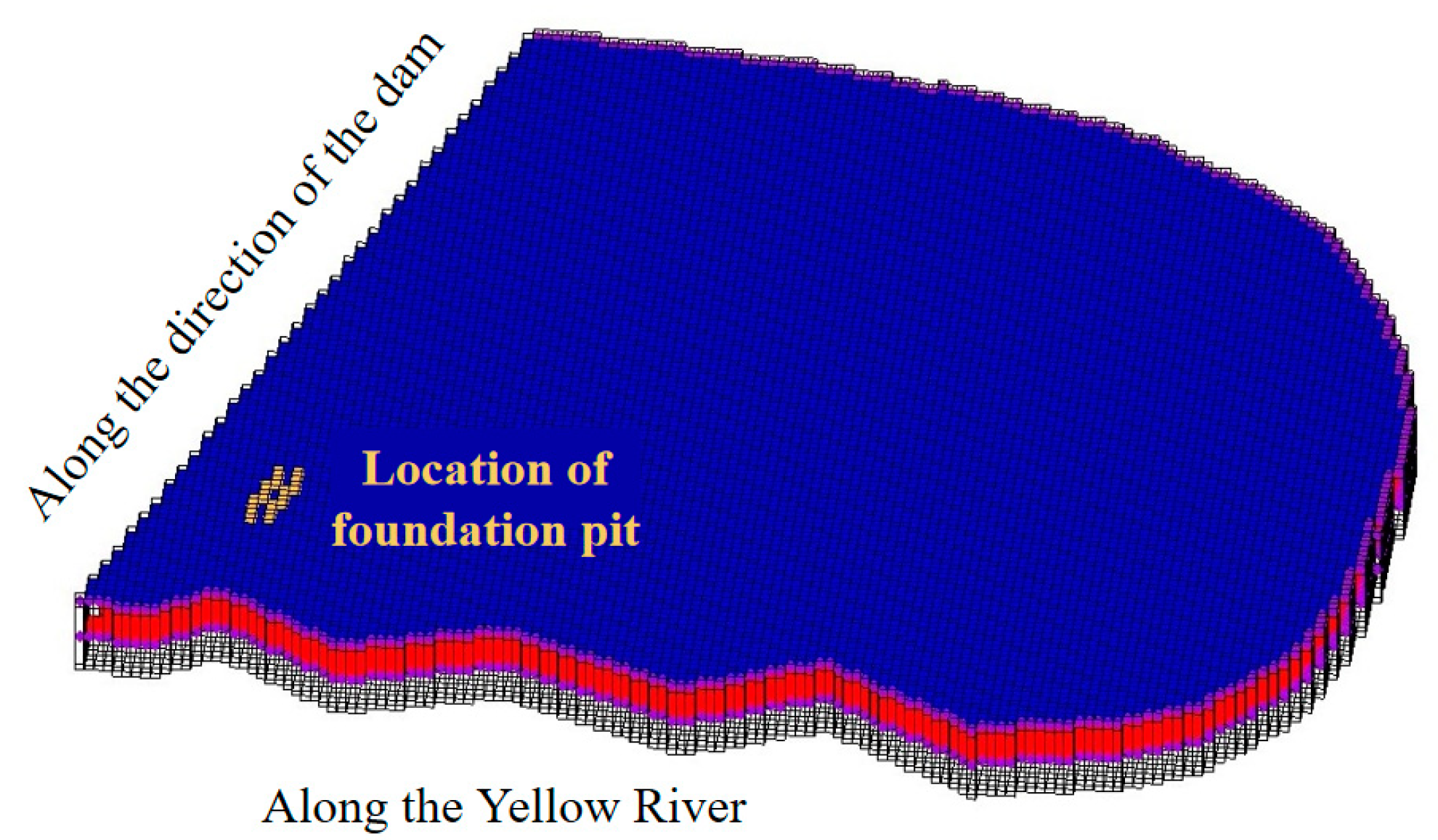
6.1. Element Subdivision of Numerical Model and Determination of Boundary Conditions

Based on the hydrogeological conditions in the study area, a numerical model is established using GMS software. The model is divided into two layers, each of which is divided into 22,500 element meshes of 150 $\times$ 150. The first layer is a sandy loam layer (119.5–122.5 m), the second layer is a pebble layer (99.5–119.5 m), and the bottom is a claystone layer. The terrain is flat, so it is treated as a horizontal layer. The vertical thickness of the overall model is 23 m. The southwest of the foundation pit in the study area is close to the Yellow River, and the fixed water head boundary is set according to the measured water level of the Yellow River during the simulation period. The Xixiayuan reservoir dam is located in the northwest, which is regarded as the impermeable boundary treatment. The poor permeability of the bottom claystone layer is regarded as the impermeable boundary, and the remaining boundaries are determined as the constant water head boundary according to the influence radius of pumping, which is set to be equal to the initial head of the study area. The grid division of the 3D geological model in the study area is shown in Figure 11. Specifically, the water level values of all constant water head boundaries in the numerical model are consistent with those taken in the optimization algorithm.

The hydrogeological parameters and physical mechanical parameters of each layer are obtained according to the survey reports and on-site slug test results, as shown in

Table 11. Hydrogeological parameters and physical and mechanical parameters of each layer.

Aquifer	Permeability Coefficient K/(m/d)	Specific Yield	Porosity	Elastic Water Storage Rate ${\mathit{S}}_{\mathit{s}\mathit{k}\mathit{e}}$ (1/m)	Inelastic Water Storage Rate ${\mathit{S}}_{\mathit{s}\mathit{k}\mathit{v}} (1/\mathbf{m})$
Sandy loam soil layer	0.35	0.05	0.3	6 × 10−4	1.2 × 10−3
Pebble layer	432	0.2	0.4	1.2 × 10−4	1.6 × 10−4

.

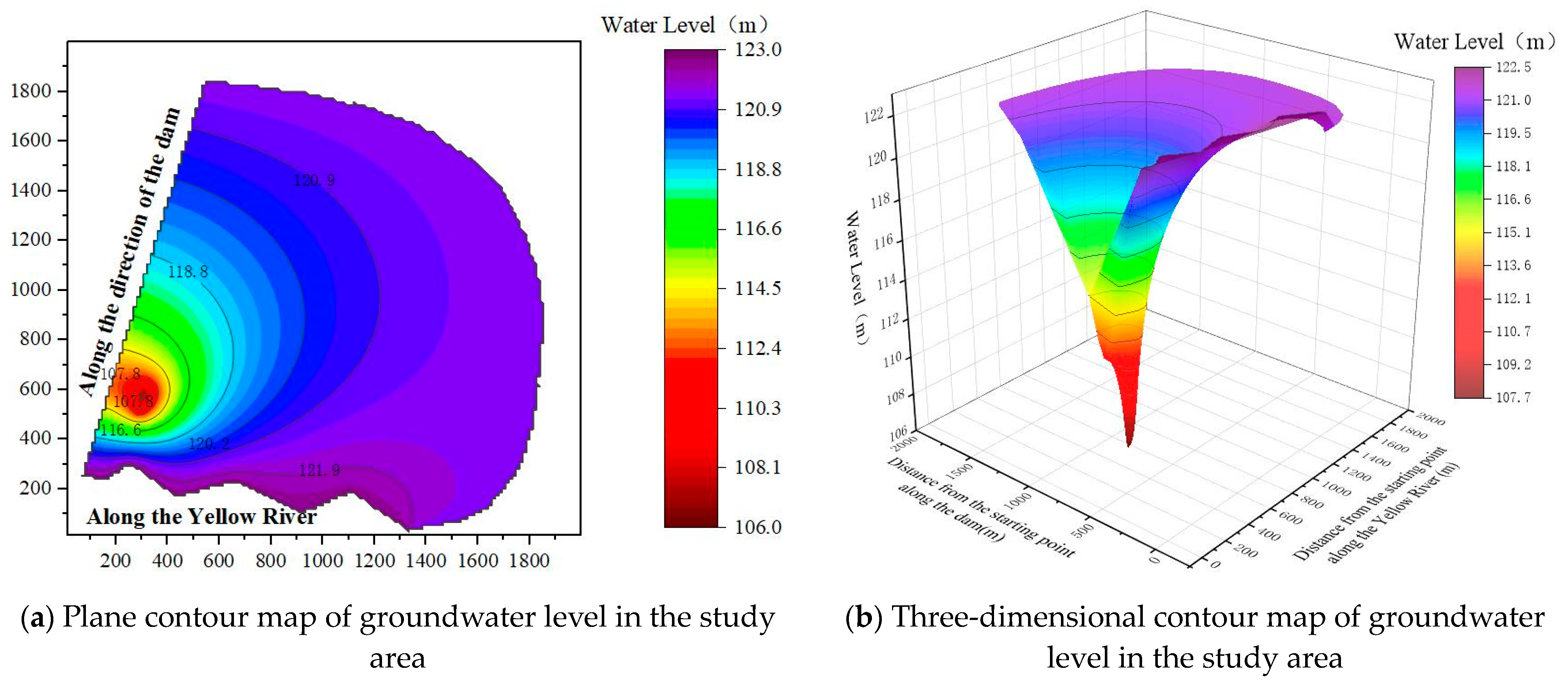
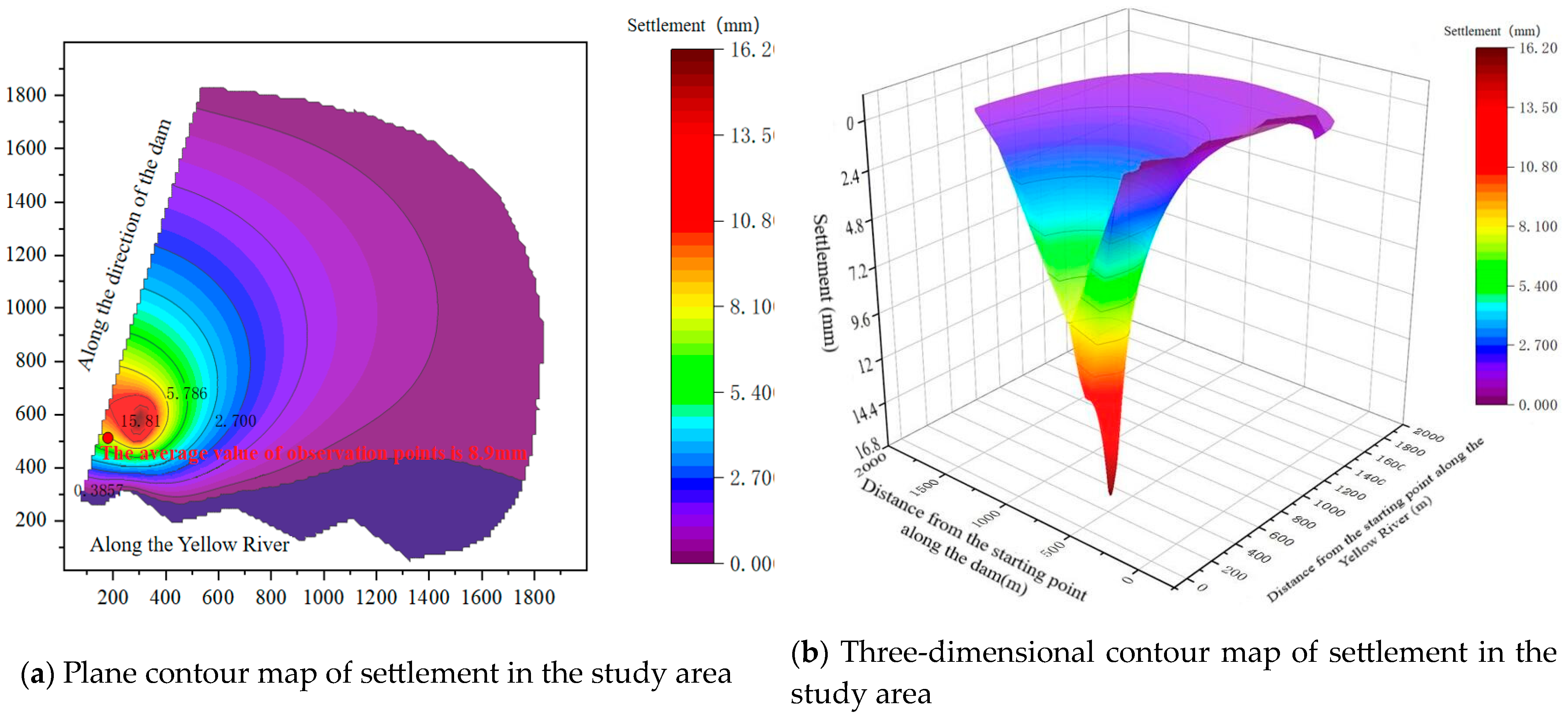
6.2. Numerical Simulation Results and Analysis

Based on the MODFLOW module and SUB subroutine package in GMS, according to the requirements of foundation pit dewatering and settlement control, and comprehensively considering three objectives, the dewatering scheme of running 24 pumping wells and closing the J19 and J22 pumping wells under the third optimal condition is numerically simulated and analyzed to verify its feasibility and accuracy. Therefore, the groundwater level and settlement contour maps in the study area under this dewatering scheme are shown in Figure 12 and Figure 13.

It can be seen from Figure 12 that the water level at the groundwater level control point in the foundation pit is lower than the elevation 110.3 m of the foundation pit bottom, and the water level in the pit is stable between 108.9 and 109.6 m, which can lower the water level to 1.4 m below the foundation pit bottom plate and meet the construction requirements.

It can be seen from Figure 13 that the settlement in the foundation pit settlement observation points is up to 8.8–9.0 mm, and the average settlement is about 8.9 mm. Compared with the allowable settlement of 15 mm calculated by the layered summation method, the simulation results show that the settlement is far less than the allowable settlement, which can reduce about 41% of the settlement. It can be verified that the optimized dewatering scheme of running 24 pumping wells and closing the J19 and J22 pumping wells under the third optimal working condition will not cause settlement damage to the foundation pit and surrounding buildings, and this can ensure construction safety.

The numerical simulation results and optimization results under this dewatering scheme are compared and analyzed, and the comparison results are shown in

Table 12. Verification and comparison of different results under the third optimal working condition.

Types	The Distance Where Water Level in the Center of the Foundation Pit Is Lower than the Bottom Plate/(m)	Mean Value of Ground Settlement Observation Points/(mm)	Total Pumping Wells Flow/(m3/d)
Allowable value	>0	<15	<144,000
Optimal results	1.84	7.95	143,665
Numerical simulation results	1.40	8.9	143,815

. The comparison results show that the numerical simulation results can lower the water level in the center of the foundation pit to 1.4 m below the bottom of the foundation pit and meet the requirements of water level drawdown. The observed value of settlement is 8.9 mm, which is less than the allowable value of 15 mm of settlement, which verifies the feasibility of the optimization results.

7. Conclusions

(1)

The objective function method is used to establish the multi-objective optimization mathematical model of foundation pit dewatering. Combined with the non-dominated sorting genetic algorithm NSGA-II and MATLAB optimization toolbox, the Gamultiobj program is called to develop an iterative program to optimize the pumping capacity of a single well and the number of pumping wells, and the solving process is given. The advantages of multi-objective optimization based on NSGA-II are that the uniformly distributed Pareto optimal solution set can be obtained, and multi-objective optimization problems for foundation pit dewatering can more quickly and efficiently be handled based on the fast-elite selection strategy. Using the Analytic Hierarchy Process (AHP) combined with the evaluation scoring method to establish an evaluation system, the candidate set with high scores in the Pareto solution set is used as the decision-making basis. The construction of an evaluation system combining NSGA-II and AHP applied in foundation pit dewatering engineering represents an innovative technology and method.

(2)

Using the NSGA-II algorithm and MATLAB optimization toolbox programming, the dewatering optimization of the foundation pit project of the inverted siphon section of the canal head (pile No. XZ0+326–XZ0+500) in the water conservancy and irrigation area engineering of the Xixiayuan water conservancy project was carried out, and the Pareto optimal solution set under three optimal conditions (24 to 26 pumping wells in running) was obtained. By incorporating the dewatering multi-objective optimization evaluation system based on the Analytic Hierarchy process, the optimization scheme within the set of Pareto optimal solutions is chosen as the ultimate decision for optimization. This scheme takes into account three objectives: the total dewatering cost, the settlement influence coefficient, and the safety and stability of the foundation pit structure. Consequently, it offers a range of workable plans for the construction of the foundation pit dewatering.

(3)

The study area’s numerical model is created using the MODFLOW module and SUB subroutine package within GMS. The optimization outcomes for the decision variables in the dewatering scheme, which involves operating 24 pumping wells and closing the J19 and J22 pumping wells based on the third optimal condition, are applied to the numerical model. The numerical simulation of this optimized scheme validates the scientific nature and accuracy of the multi-objective optimization model for foundation pit dewatering. Importantly, the established multi-objective optimization model and evaluation system offer numerous viable dewatering optimization plans.

References

1. Zhang, Y.Q.; Li, M.G.; Wang, J.H.; Chen, J.J.; Zhu, Y.F. Field tests of pumping-recharge technology for deep confined aquifers and its application to a deep excavation. Eng. Geol. 2017, 228, 249–259. [Google Scholar] [CrossRef]
2. Sharifi, M.R.; Akbarifard, S.; Madadi, M.R.; Qaderi, K.; Akbarifard, H. Optimization of hydropower energy generation by 14 robust evolutionary algorithms. Sci. Rep. 2022, 12, 7739. [Google Scholar] [CrossRef]
3. Wang, X.L.; Li, S.H.; Chen, H.Y.; Wang, X.F.; Mei, Y. Multi-objective and multi region power grid planning based on non dominated genetic algorithm and coevolutionary algorithm. Proceeding CSEE 2006, 12, 11–15. [Google Scholar]
4. Xu, Y.; Yan, Y. Optimal Design of Foundation Pit Dewatering Based on Objective Functions and Numerical Analysis. Adv. Mater. Res. 2011, 368–373, 2495–2499. [Google Scholar] [CrossRef]
5. Liu, J.; Luo, X. Application of Genetic Algorithm in Deep Foundation Pit Dewatering. Site Investig. Sci. Technol. 2000, 3, 42–45. [Google Scholar]
6. Yang, Y.; Wu, J.; Sun, X.; Wu, J.; Zheng, C. Development and application of a master-slave parallel hybrid multi-objective evolutionary algorithm for groundwater remediation design. Environ. Earth Sci. 2013, 70, 2481–2494. [Google Scholar] [CrossRef]
7. Wahid, F.; Alsaedi, A.K.Z.; Ghazali, R. Using improved firefly algorithm based on genetic algorithm crossover operator for solving optimization problems. J. Intell. Fuzzy Syst. 2019, 36, 1547–1562. [Google Scholar] [CrossRef]
8. Geng, J.; Cui, Z.; Gu, X. Scatter search-based particle swarm optimization algorithm for earliness/tardiness flow shop scheduling with uncertainty. Int. J. Autom. Comput. 2016, 13, 285–295. [Google Scholar] [CrossRef]
9. Li, N.; Zou, T.; Sun, D. Multi-objective optimization algorithm based on particle swarm optimization. Comput. Eng. Appl. 2005, 23, 43–46. [Google Scholar]
10. Ma, C. Multi-Objective Optimization of Subway Construction Projects Based on Improved Genetic Algorithm. Ph.D. Thesis, Lanzhou Jiaotong University, Lanzhou, China, 2020. [Google Scholar]
11. Khodadadi, N.; Azizi, M.; Talatahari, S.; Sareh, P. Multi-Objective Crystal Structure Algorithm (MOCryStAl): Introduction and Performance Evaluation. IEEE Access 2021, 9, 117795–117812. [Google Scholar] [CrossRef]
12. Abdel-Basset, M.; Mohamed, R.; Mirjalili, S.; Chakrabortty, R.K.; Ryan, M. An Efficient Marine Predators Algorithm for Solving Multi-Objective Optimization Problems: Analysis and Validations. IEEE Access 2021, 9, 42817–42844. [Google Scholar] [CrossRef]
13. Sang-To, T.; Le-Minh, H.; Wahab, M.A.; Thanh, C.-L. A new metaheuristic algorithm: Shrimp and Goby association search algorithm and its application for damage identification in large-scale and complex structures. Adv. Eng. Softw. 2023, 176, 103363. [Google Scholar] [CrossRef]
14. Sang-To, T.; Le-Minh, H.; Mirjalili, S.; Wahab, M.A.; Cuong-Le, T. A new movement strategy of grey wolf optimizer for optimization problems and structural damage identification. Adv. Eng. Softw. 2022, 173, 103276. [Google Scholar] [CrossRef]
15. Prina, M.G.; Cozzini, M.; Garegnani, G.; Manzolini, G.; Moser, D.; Oberegger, U.F.; Pernetti, R.; Vaccaro, R.; Sparber, W. Multi-objective optimization algorithm coupled to EnergyPLAN software: The EPLANopt model. Energy 2018, 149, 213–221. [Google Scholar] [CrossRef]
16. Zhang, X.; Liu, H.; Tu, L. A modified particle swarm optimization for multimodal multi-objective optimization. Eng. Appl. Artif. Intell. 2020, 95, 103905. [Google Scholar] [CrossRef]
17. Srinivas, N.; Deb, K. Muiltiobjective Optimization Using Nondominated Sorting in Genetic Algorithms. Evol. Comput. 1994, 2, 221–248. [Google Scholar] [CrossRef]
18. Xu, T.; He, J.; Shang, C.; Ying, W. A New Multi-objective Model for Constrained Optimisation. In Advances in Computational Intelligence Systems; Springer: Cham, Switzerland, 2017; pp. 71–85. [Google Scholar] [CrossRef]
19. Mirjalili, S.Z.; Mirjalili, S.; Saremi, S.; Faris, H.; Aljarah, I. Grasshopper optimization algorithm for multi-objective optimization problems. Appl. Intell. 2018, 48, 805–820. [Google Scholar] [CrossRef]
20. Wang, X.; Li, S. Multi-Objective Optimization Using Cooperative Garden Balsam Optimization with Multiple Populations. Appl. Sci. 2022, 12, 5524. [Google Scholar] [CrossRef]
21. Zhang, K.; Chen, M.; Xu, X.; Yen, G.G. Multi-objective evolution strategy for multimodal multi-objective optimization. Appl. Soft Comput. J. 2021, 101, 107004. [Google Scholar] [CrossRef]
22. Dhiman, G.; Singh, K.K.; Soni, M.; Nagar, A.; Dehghani, M.; Slowik, A.; Kaur, A.; Sharma, A.; Houssein, E.H.; Cengiz, K. MOSOA: A new multi-objective seagull optimization algorithm. Expert Syst. Appl. 2021, 167, 114150. [Google Scholar] [CrossRef]
23. Jamil, M.A.; Nour, M.K.; Alotaibi, S.S.; Hussain, M.J.; Hussaini, S.M.; Naseer, A. Software Product Line Maintenance Using Multi-Objective Optimization Techniques. Appl. Sci. 2023, 15, 9010. [Google Scholar] [CrossRef]
24. Guan, Y.; Chu, Y.; Lv, M.; Li, S.; Li, H.; Dong, S.; Su, Y. Application of Strength Pareto Evolutionary Algorithm II in Multi-Objective Water Supply Optimization Model Design for Mountainous Complex Terrain. Sustainability 2023, 15, 12091. [Google Scholar] [CrossRef]
25. Huynh, T.Q.; Nguyen, T.T.; Nguyen, H. Base resistance of super-large and long piles in soft soil: Performance of artificial neural network model and field implications. Acta Geotechica 2023, 18, 2755–2775. [Google Scholar] [CrossRef]
26. Li, Y.; Hariri-Ardebili, M.A.; Deng, T.; Wei, Q.; Cao, M. A surrogate-assisted stochastic optimization inversion algorithm: Parameter identification of dams. Adv. Eng. Inform. 2023, 55, 101853. [Google Scholar] [CrossRef]
27. Wu, J.; Zhu, X. Development trend of groundwater flow numerical simulation software based on MODFLOW. Eng. Investig. 2000, 2, 12–15. [Google Scholar]
28. Rong, Y.; Fang, Z. Risk assessment of ground settlement induced by construction dewatering of Taizhou Bridge anchorage caisson foundation. In Proceedings of the 2011 Second International Conference on Mechanic Automation and Control Engineering, Huhhot, China, 15–17 July 2011. [Google Scholar] [CrossRef]
29. Corne, D.W.; Knowles, J.D.; Oates, M.J. The Pareto envelope-based selection algorithm for multiobjective optimization: International Conference on Parallel Problem Solving from Nature. Lect. Notes Comput. Sci. 2000, 1917, 839–848. [Google Scholar]
30. Sharma, S.; Kumar, V. A Comprehensive Review on Multi-objective Optimization Techniques: Past, Present and Future. Arch. Comput. Methods Eng. 2022, 29, 5605–5633. [Google Scholar] [CrossRef]
31. Shi, F. Analysis of 30 Cases of MATLAB Intelligent Algorithms [M]; Beijing University of Aeronautics and Astronautics Press: Beijing, China, 2011. [Google Scholar]
32. Furtuna, R.; Curteanu, S.; Leon, F. An elitist non-dominated sorting genetic algorithm enhanced with a neural network applied to the multi-objective optimization of a polysiloxane synthesis process. Eng. Appl. Artif. Intell. 2011, 24, 772–785. [Google Scholar] [CrossRef]
33. JGJ/120-2012; Technical Regulations for Building Foundation Pit Support. Ministry of Housing and Urban-Rural Development, People’s Republic of China: Beijing, China, 2012.
34. GB50202-2018; The Construction Quality Acceptance Code for Building Foundation Engineering. Ministry of Housing and Urban-Rural Development, People’s Republic of China: Beijing, China, 2018.
35. Zhao, Y.; Dong, X.; Wang, H.; Wang, J.; Wei, Y.; Huang, Y.; Xue, R. Comparative Study on the Application of Different Slug Test Models for Determining the Permeability Coefficients of Rock Mass in Long-Distance Deep Buried Tunnel Projects. Appl. Sci. 2022, 12, 10235. [Google Scholar] [CrossRef]
36. Zhao, Y.; Wang, H.; Lv, P.; Dong, X.; Huang, Y.; Wang, J.; Yang, Y. Theoretical Model and Experimental Research on Determining Aquifer Permeability Coefficients by Slug Test under the Influence of Positive Well-Skin Effect. Water 2022, 14, 3089. [Google Scholar] [CrossRef]
37. Zhao, Y.; Wei, Y.; Dong, X.; Rong, R.; Wang, J.; Wang, H. The Application and Analysis of Slug Test on Determining the Permeability Parameters of Fractured Rock Mass. Appl. Sci. 2022, 12, 7569. [Google Scholar] [CrossRef]
38. Zhao, Y.; Zhang, Z.; Rong, R.; Dong, X.; Wang, J. A new calculation method for hydrogeological parameters from unsteady-flow pumping tests with a circular constant water-head boundary of finite scale. Q. J. Eng. Geol. Hydrogeol. 2022, 55, qjegh2021-112. [Google Scholar] [CrossRef]
Figure 1. NSGA-II algorithm flow chart.
Applsci 13 10865 g001
Figure 2. Technical route for optimal solution of multi-objective optimization model of foundation pit dewatering based on NSGA-II algorithm.
Applsci 13 10865 g002
Figure 3. Location distribution map of study area.
Applsci 13 10865 g003
Figure 4. Engineering geological longitudinal section and foundation pit location of canal head inverted siphon section XZ0+326–XZ0+500.
Applsci 13 10865 g004
Figure 5. Pareto set distribution diagram and pumping well working state under the first optimized working condition. (In the figure (a), the red dot indicates the relationship between the total water inflow and the settlement influence coefficient, the green dot indicates the relationship between the central water level drawdown and the total water inflow, the blue dot indicates the relationship between the central water level drawdown and the settlement influence coefficient).
Applsci 13 10865 g005
Figure 6. Optimization results of decision variables under the first optimization working condition.
Applsci 13 10865 g006
Figure 7. Pareto set distribution diagram and pumping well working state under the second optimal working condition. (In the figure (a,c,e), the red dot indicates the relationship between the total water inflow and the settlement influence coefficient, the green dot indicates the relationship between the central water level drawdown and the total water inflow, the blue dot indicates the relationship between the central water level drawdown and the settlement influence coefficient).
Applsci 13 10865 g007
Figure 8. Optimization results of decision variables under the second optimization working condition.
Applsci 13 10865 g008
Figure 9. Pareto set distribution diagram and pumping well working state under the third optimal working condition. (In the figure (a,c,e), the red dot indicates the relationship between the total water inflow and the settlement influence coefficient, the green dot indicates the relationship between the central water level drawdown and the total water inflow, the blue dot indicates the relationship between the central water level drawdown and the settlement influence coefficient).
Applsci 13 10865 g009
Figure 10. Optimization results of decision variables under the third optimization working condition.
Applsci 13 10865 g010
Figure 11. Grid division of 3D geological model of the study area.
Applsci 13 10865 g011
Figure 12. Contour map of groundwater level in the study area.
Applsci 13 10865 g012
Figure 13. Contour map of settlement in the study area.
Applsci 13 10865 g013