Article

Evaluating the Influence of Sand Particle Morphology on Shear Strength: A Comparison of Experimental and Machine Learning Approaches

by
Firas Daghistani
1,2 and
Hossam Abuel-Naga
1,*
1
Department of Civil Engineering, La Trobe University, Bundoora, VIC 3086, Australia
2
Department of Civil Engineering, University of Business and Technology, Jeddah 21448, Saudi Arabia
*
Author to whom correspondence should be addressed.
Appl. Sci. 2023, 13(14), 8160; https://doi.org/10.3390/app13148160
Submission received: 7 June 2023 / Revised: 10 July 2023 / Accepted: 11 July 2023 / Published: 13 July 2023
(This article belongs to the Special Issue The Application of Machine Learning in Geotechnical Engineering)

Abstract

:
Particulate materials, such as sandy soil, are everywhere in nature and form the basis for many engineering applications. The aim of this research is to investigate the particle shape, size, and gradation of sandy soil and how they relate to shear strength, which is an essential characteristic that impacts soil stability and mechanical behaviour. This will be achieved by employing a combination of experimental methodology, which includes the use of a microscope direct shear apparatus, and machine learning techniques, namely multiple linear regression and random forest regression. The experimental findings reveal that angular-shaped sand particles enhance the shear strength characteristics compared to spherical, rounded ones. Similarly, coarser sand particles improve these characteristics compared to finer sand particles, as do well-graded particles when compared to poorly graded ones. The machine learning findings show the validity of both models in predicting shear strength when compared to the experimental results, showing high accuracy. The models are designed to predict shear strength of sand considering six input features: mean particle size, uniformity coefficient, curvature coefficient, dry density, normal stress, and particle regularity. The most important features from both models were identified. In addition, an empirical equation for calculating shear strength was developed through multiple linear regression analysis using the six features.

1. Introduction

Natural particulate materials, such as sandy soil, are found everywhere and are essential to many engineering applications. Various fields, from civil engineering to materials science, require an understanding of the mechanical behaviour of particle-to-particle [1,2] and their interactions with different surfaces [3,4,5,6]. Understanding these materials is strongly reliant on particle morphology, which has a significant influence on the mechanical response of granular materials such as sand. The term ‘particle morphology’ is used to refer to particle shape, size, form, sphericity, or surface roughness. With regards to particle size, the soil size in descending order is boulder, cobbles, pebbles, gravel, sand, silt, and clay. The scope of this paper will be limited to sand, which is a granular material composed of individual particles classified into three sizes: coarse, medium, and fine sand, as specified by the Australian standard [7].
While the particle shape has been a topic that has raised many questions in the literature, its implication on the behaviour of soil is a major area of study with constant research progression. The soil particle shape can be graded on three independent properties: form (sphericity: overall shape), roundness, and roughness, each of which has a different influence on the behaviour of the material [8]. With regards to the sphericity, the soil particles can be bulky, flaky, and needle shaped. Sand particles are considered bulky, and their shape is mostly set during formation. Researchers often use terms such as ‘well-rounded’, ‘rounded’, ‘sub-rounded’, ‘subangular’, ‘angular’, and ‘very angular’ to describe the roundness of bulky particles. However, the sand’s surface roughness can change significantly with mechanical and chemical weathering of rocks and minerals over geological time [9]. While sphericity and roundness are macro- and medium-scale particle measurements, particle surface texture is a microscale measurement [10]. With regards to granular sand, the particle shape, including sphericity, roundness, and roughness, affect the sand’s stiffness, strength, minimum and maximum void ratio (e min and e max), critical state friction angle (φ c), dilatancy (ψ), dilation, strain localisation, and the evolution of strength anisotropy [11]. Furthermore, particle shape can significantly influence the compressibility of granular structures. Experimental studies have found that particle roundness and sphericity (particle regularity) can affect both packing density and compressibility [2].
The shape of soil particles, including roundness, angularity, and surface roughness, plays a significant role in determining soil mechanical behaviour. Roundness impacts how particles interact, affecting soil mass packing and stiffness [12,13,14]. Angular particles, due to their enhanced interlocking, exhibit higher friction angles and shear strength [15]. Li [16] found that as sample convexity decreased, friction angle increased. This statement was supported by an experimental and numerical study by Peng et al. [17], whose results showed that angular particles have more shear strength compared to rounded particles. Surface roughness influences soil stiffness [18] and wave propagation parameters [19]. Angularity affects the undrained response of fine sands, with more angular particles offering increased resistance to movement, thereby boosting soil strength [20,21]. The work of researchers like Miura et al. [22] in studying the impact of these properties on soil behaviour contributes to more accurate predictive models, directly informing engineering practices.
Particle size has an important effect on the behaviour of individual particles and the packaging density. Vangla and Latha [23] investigated the effect of particle size on shear strength characteristics. They attempted to eliminate the effect of morphological characteristics by selecting three sands with different particle sizes (coarse, medium, and fine) but similar particle shapes (angularity, roundness, sphericity, and roughness). The samples were prepared at a similar void ratio, and the test was carried out using direct shear. The results showed that particle size has a slight influence on the peak friction angle but not on the mechanism of shearing, with coarse sand particles taking longer to reach the peak compared to fine sand particles. In contrast, an experiment by Wang et al. [24] investigated the effect of sand and gravel size on shear strength using both direct shear and triaxial tests in the laboratory. The results showed that as the mean particle diameter D50 increased, the angle of shearing resistance also increased, leading to higher shear strength. Similar results were reported by [16,25,26], who found that peak and residual shear strength increase as particle size increases, whereas in glass beads, interparticle friction between two glass beads increases as sphere size increases [27]. Interestingly, particle size also affects the compressibility of the granular structure, with smaller particles leading to greater compression compared to larger particles [1].
Researchers in the engineering, geotechnics, as well as the medical field have become more interested in artificial intelligence (AI) techniques over the last two decades. A variety of machine learning algorithms have been utilised with significant success, including multiple linear regression (MLR) and random forest regression (RFR), which we have adopted in our research. In a study by Xie et al. [28], the two models, MLR and RF, were compared for estimating soil extracellular enzyme activities in reclaimed coastal saline land. The authors report that the RF model performed better than the MLR model in predicting the activities of soil amylase and urease, which are important indicators of soil carbon and nitrogen cycling. The article also identifies the main factors affecting soil extracellular enzyme activities, such as soil water content, total nitrogen, and pH. Another study by Zhang et al. [29], who also used MLR and RF models, investigated the prediction of soil organic carbon (SOC) in a coastal reclamation zone of eastern China. The authors compared the effects of different factors on SOC dynamics and found that soil pH, chloride, and silt contents were the most important factors influencing SOC. Results from the study indicated that the RF model also performed better than MLR due to its superiority in handling non-linear relationships between SOC and the predictors. The RF model showed substantially reduced error indices (ME, MSE, and RMSE), as well as a higher R2. Another interesting technique is the Adaptive Neuro-Fuzzy Inference System (ANFIS) introduced by Jang in 1993. ANFIS integrates the elements of neural networks and fuzzy logic, demonstrating capabilities of learning and generalisation [30]. The system has found diverse applications across various domains. It has been used for predicting skin permeability in drug-delivery scenarios [31], controlling quality and predicting characteristics in food-processing technology [32], determining heavy metal concentrations in water resources [33], and even predicting the security index of ad hoc vehicular networks [34]. Moreover, it has shown efficacy in predicting the higher heating value of biomass [35] and modelling thermal error [36]. In addition, a recent article [37] presents a method to control the cooling of machine tool spindles using ANFIS. The method adjusts the coolant pump frequency based on the spindle speed and thermal state, achieving high accuracy and efficiency in reducing thermal deformation and energy consumption. While MLR and RFR provide robust and interpretable models, the potential of ANFIS, given its successful implementation in various studies, indicates it as an intriguing future direction for predictive modelling research, including predicting the shear strength of cohesionless soil.
The analysis of shear strength of cohesionless soil such as sand can be influenced by granular shape, size, and gradation. However, no comprehensive model taking these parameters into account can be found in the literature. This is because there are many variables that affect it in non-linear ways. In the geotechnical field, machine learning has been used successfully for problems such as slope stability [38], soil mechanics [39,40], soil cracking [41], and soil improvement with recycled materials [42,43,44,45,46]. However, the application of AI methodologies for predicting the shear strength of cohesionless soil, considering the combined influence of particle shape, size, and gradation, has not been sufficiently investigated, indicating a large gap in past research. This research aims to fill this gap by conducting and analysing a series of direct shear tests across different granular sizes and shapes. This is followed by the application of both MLR and RFR, which are based on six input features: mean particle size (D50), coefficient of uniformity (Cu), coefficient of curvature (Cc), dry density (Ꝭd), normal stress (σn), and particle regularity ( r ) , the last of which is the average of roundness and sphericity. The research then presents an empirical equation for predicting the shear strength of sand, considering the six input features. Finally, after careful examination of the results derived from the models, the study presents the most effective model and investigates the significance of the inputs involved in each model. This study provides a strong base for a deep investigation into a new area that was not explored before.

2. Materials and Methods
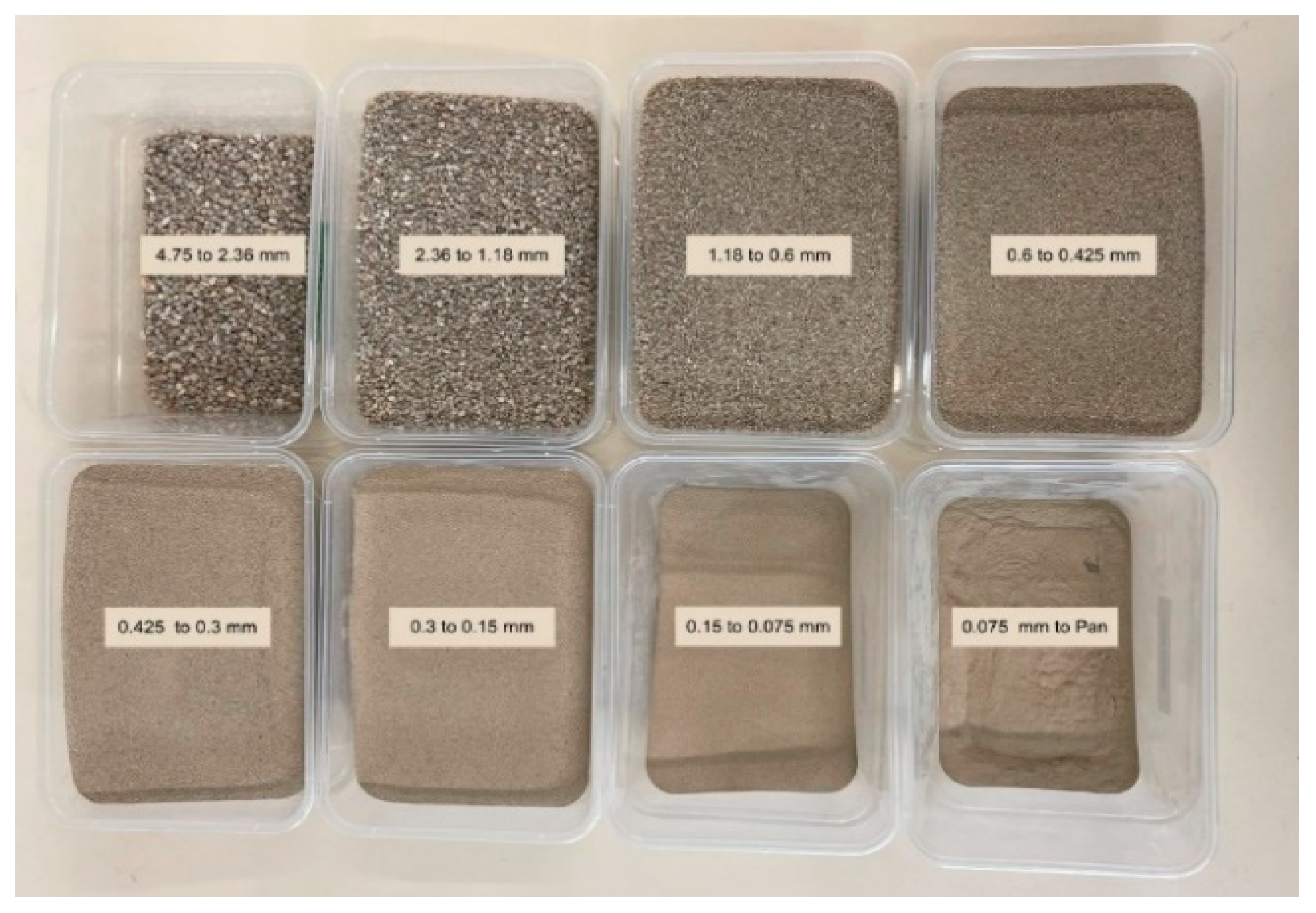
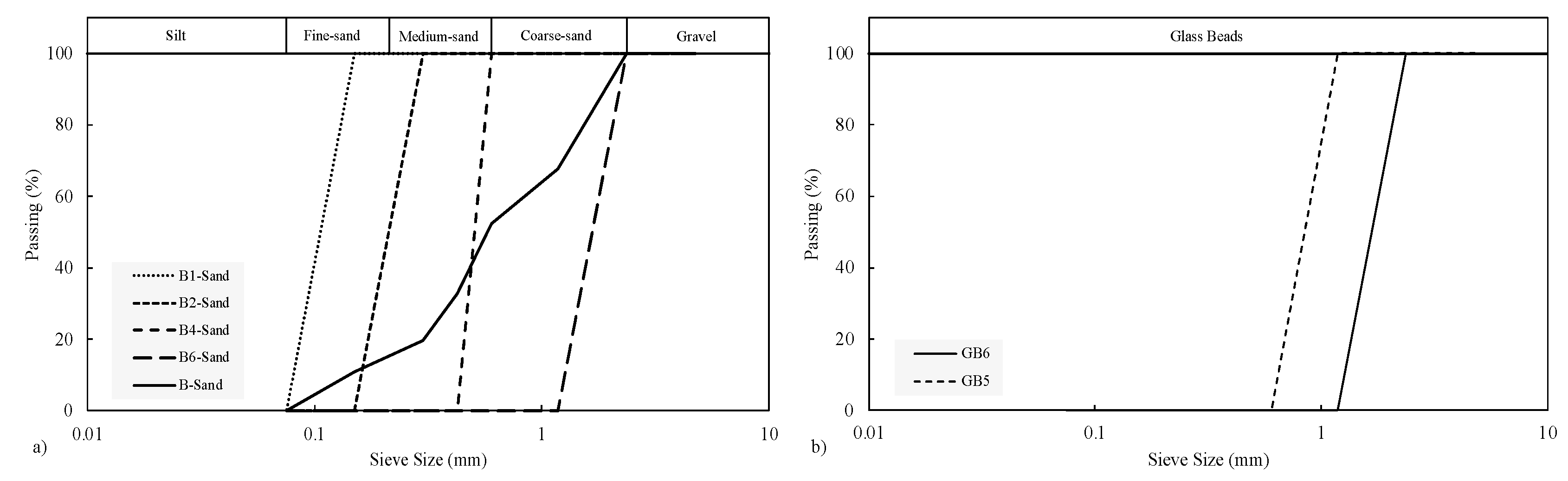
2.1. Material

According to the Australian standard [7], sand sizes range from 2.36 mm to 0.075 mm, with coarse sand ranging from 2.36 to 0.6 mm, medium sand ranging from 0.6 to 0.212 mm, and fine sand ranging from 0.212 to 0.075 mm. Particles larger than 2.36 mm are classified as gravel, while particles smaller than 0.075 mm are classified as silt or clay. Different types of sand were used in the experiments to examine the effect of particle size and shape. The sands used in the study are referred to as L-Sand, M-Sand, P-Sand, and B-Sand.
For the particle shape impact, four types of sand were used, namely L-Sand, B-Sand, M-Sand, and P-Sand, were each sieved and separated into four different sizes (1.18 to 0.6 mm, 0.6 to 0.425 mm, 0.425 to 0.3 mm, and 0.3 to 0.15 mm). Due to the limitation of the microscope lens, which tends to overlook particles larger than 1.18 mm, only particles below this size were selected.
To study the impact of particle size, B-sand was sieved and divided into containers based on their size (Figure 1), and five different sands were selected for testing. According to Australian standards [7], four of the selected sands are poorly graded and are considered to be fine sand (B1-Sand) with D50 of 0.11 mm, low medium sand (B2-Sand) with D50 of 0.23 mm, high medium sand (B4-Sand) with D50 of 0.51 mm, and coarse sand (B6-Sand) with D50 of 1.77 mm. The fifth one is a mixture of sand to create a well-graded sand (B-Sand) with D50 of 0.58 mm. Therefore, five different sizes were chosen to examine the differences between coarse, medium, and fine sands, as well as to study the effect of poorly graded and well-graded sands.
Glass beads were utilised to avoid particle shape influence and concentrate only on particle size impact on mechanical behaviour. The glass beads are made of silica mixed with other minerals melted at high temperature to produce a viscous, thick liquid. The liquid is moulded into spherical shapes and hardens as it cools. The regularity of the particle shape of the glass beads, as observed under the microscope, was found to be almost one. The glass beads were separated into two different sizes: GB5 with a D50 of 0.89 mm and GB6 with a D50 of 1.77 mm. The specific gravity of the glass beads ranges from 2.45 to 2.50. The specifications of used particulate materials including sand and glass beads are presented in Table 1. The sieve analysis was conducted according to the Australian standard [47], and the results for the used granular material are shown in Figure 2.

2.2. Experimental

A total of 1068 tests, including microscopy, direct shear, oedometer, and specific gravity tests, were conducted. Out of these experiments, 1000 involved photographing various types of sand, which include L-Sand, M-Sand, P-Sand, and B-Sand. Each of these sands was sieved and separated into different containers based on their sizes. Subsequently, microscope analysis was performed on uniformly sized specimens. We considered 50 particles in each specimen in order to determine particle regularity. Additionally, 46 direct shear tests were conducted, considering different particle sizes, shapes, and densities. Further, six tests were carried out to measure compressibility across varying particle sizes and densities using an oedometer apparatus. Lastly, 16 tests were conducted to determine the specific gravity of different types of sand of various particle sizes. This was done to investigate the impact of the mean particle size on specific gravity.

2.2.1. Direct Shear Apparatus

A Mateset direct shear apparatus was used to conduct the experiments, which were carried out according to the Australian standard [48]. The dimensions of the mould in the direct shear box were 60 × 60 mm. In each test, different amounts of normal stresses, 25, 50, 100, and 200 kPa, were applied to the sample. Each test was conducted on a dry sample at a shear rate of 1 mm/min, which is the maximum allowable speed according to the standard.
The pluviation technique, sometimes called the rainfall method, is employed in the preparation of granular soil samples, specifically sands, with differing relative densities. Figure 3 provides a schematic diagram of the pluviation technique. By adjusting the height from which the sand particles are dropped, the method allows for the creation of samples with the required density.
The relationship between drop height versus void ratio and relative density is shown in Figure 4, with the void ratio decreasing as drop height increases. A loose sample is achieved by dropping the soil from a low distance between the cone and mould, reducing the particles’ kinetic energy and enabling them to loosely pack. Conversely, a dense sample is formed by dropping the particles from a high distance, increasing their kinetic energy, and causing them to efficiently rearrange and pack densely. Upon dropping the particles from the selected height, the mould is removed, and the sample can be used for shearing testing.
In the study, two different densities were considered when preparing the sample: the loose and dense density states. In the loose density state, the sand was spooned and dropped from a very low height (zero height). Conversely, in the dense state, the sample was dropped from a cone with a 5.2 mm opening at a height of 83 cm.

2.2.2. Microscope

In this experiment, we used a Nikon Eclipse MA100 microscope, a valuable tool in geotechnical laboratories for identifying particle shapes. The microscope comes with a built-in Progression system, offers high-quality optics that enable accurate and efficient identification of soil particle shapes and sizes. Several parameters are used to characterize sand particle shape and quality, including sphericity and roundness (Figure 5).
The sphericity of a particle is a measure of how closely it looks like a circle, while roundness determines how curved its corners are. A ceramic proppant and high-quality frac sand are typically both spherical and round, scoring around 0.9 in both metrics. The same high score is observed in silica sand samples with nearly circular particles, where the sphericity measure can reach 0.7 or higher. Nonetheless, sand particles featuring angular edges are expected to have reduced roundness measurements, often falling in the region of 0.2 to 0.5. The schematic representation in Figure 6 shows the method of finding particle shape parameters including roundness, sphericity, and regularity.

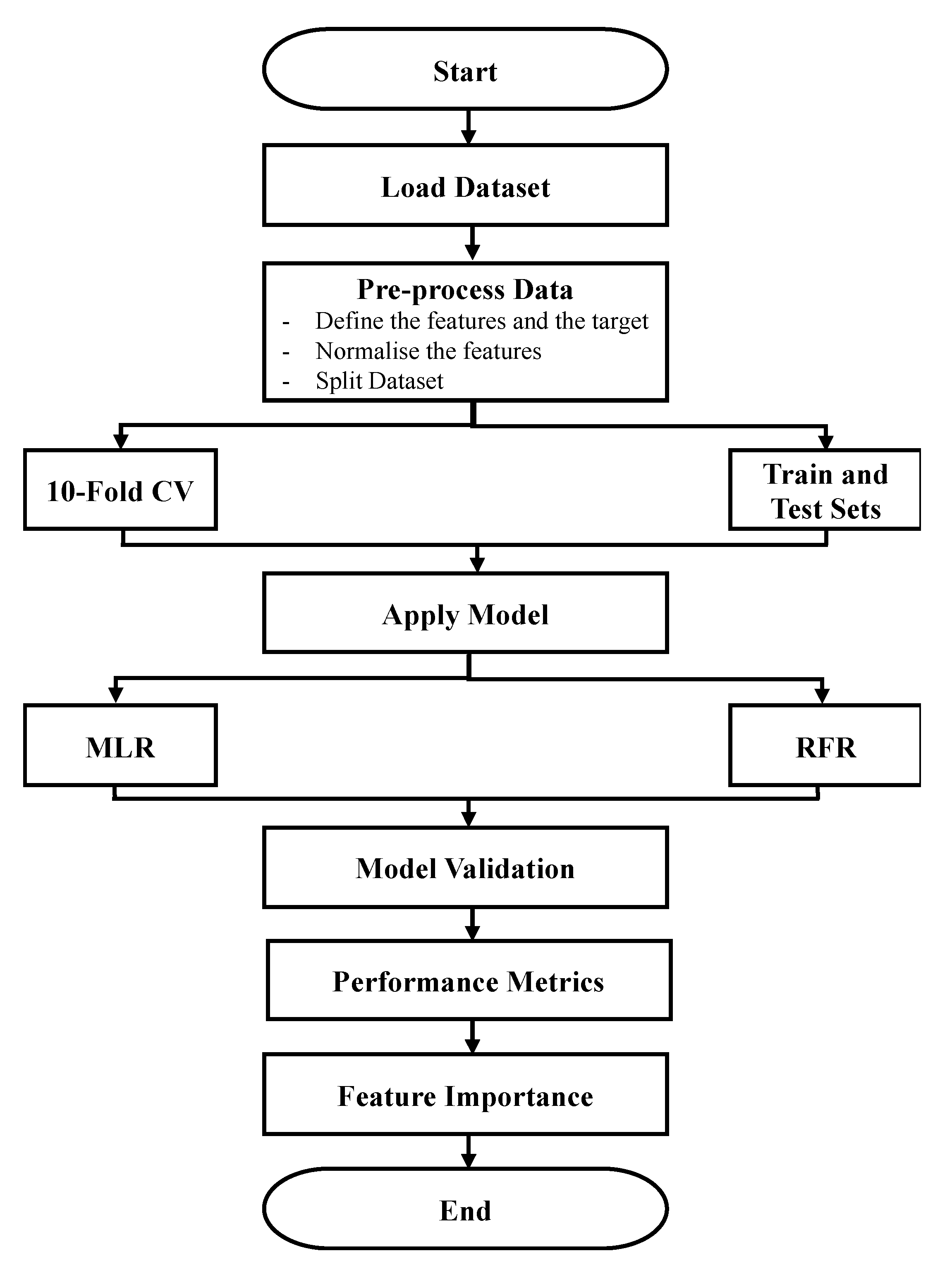
2.3. Mathematical Model

The mathematical model was implemented in the Python programming language. The research objectives entailed testing two models: a simple model via multiple linear regression (MLR), and a complex model through random forest regression (RFR). In addition, MLR was specifically applied to model linearity, while RFR was used to navigate nonlinearity. In both implemented models (MLR and RFR) the following libraries were utilised: pandas for data manipulation and analysis, NumPy for numerical computations, scikit-learn for machine learning tasks including data splitting, normalisation, regression modelling, and metric evaluation, and finally matplotlib for data visualisation. The workflow diagram below (Figure 7) outlines the different processes performed for the machine learning algorithm implementation. Further details of these processes are discussed in the following subsections.

2.3.1. Pre-Process Data

The pre-processing of data involved two steps: normalisation and splitting the dataset. Normalisation in machine learning is a vital process that standardizes numerical data in your dataset, similar to converting measurements from feet, inches, and yards all into metres, so everything is on the same scale. This process ensures that the machine learning models treat all features fairly and do not overvalue one feature while undervaluing another [50]. When all of the features are on the same scale, the model can learn and make predictions more effectively and efficiently. Techniques like min-max normalisation, Z-score normalisation, and robust scaling are commonly used. In other words, normalisation makes the data neat and uniform, helping machine learning models perform at their best.
In the results analysis, the min-max Normalisation method was followed, which rescales the data to a range between 0 and 1. The formula for this is as follows:
X = ( X X   m i n ) ( X   m a x X   m i n )
where X is the original value, and X min and X max are the smallest and largest values in the data.
Following normalisation is the splitting of the dataset. Data splitting is a popular method for model validation in which we divide a given dataset into two distinct sets: training and testing. Following that, the statistical and machine learning models are fitted to the training set and validated using the testing set. By separating a portion of the data for validation purposes, independent of the training process, we can effectively assess and compare the predictive performance of various models. The most used ratio of data splitting is 80:20, where 80% of the data is used for training and 20% for testing. This conventional method relies on a single random split of the data. The 80:20 split draws its justification from the well-known Pareto principle, which states that roughly 80% of the effects come from 20% of the causes or inputs [51]. The train–test split, although commonly used, has been found to have potential biases and limitations in assessing model performance. To overcome these challenges, we implemented the k-fold cross-validation method.
The k-fold cross-validation is a popular statistical method that provides a more comprehensive, robust, and reliable approach to assess the model’s performance and reduce computation time without any bias resulting from random dataset splitting [52,53]. This technique enables a more rigorous evaluation of the model’s effectiveness compared to the train_test_split approach.
In our own dataset, we incorporated both the train_test_split and the k-fold cross-validation (10 folds) methods. For the k-fold cross-validation, the dataset was divided into 10 sections, with nine sections used for training the model and the remaining section for testing. In each fold, a different section was designated for training, while the remaining sections were used for testing. This process was repeated across all folds until each section was used for both training and testing. The final result obtained from our 10-fold cross-validation was an average of the performance across all folds.

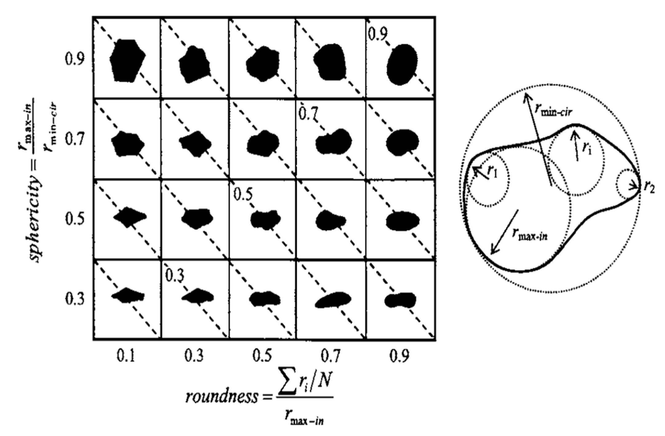
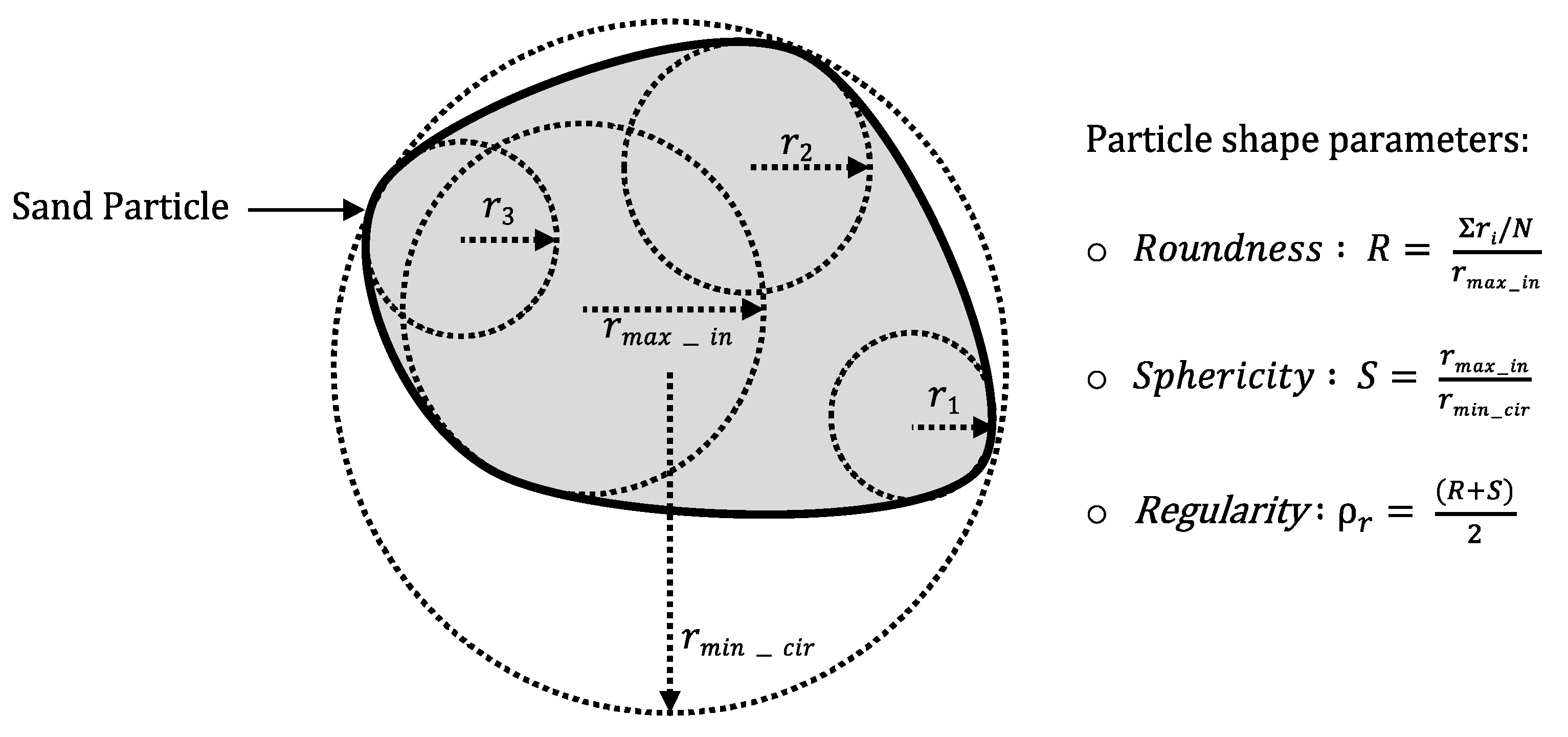
2.3.2. Statistical Parameters

Several metrics, each with its own strengths and limitations, can be used to compare the performance of various AI models. The following are some common metrics:
  • Mean absolute error (MAE) is a measure that captures the average absolute disparity between predicted and true values. By focusing solely on the magnitude of the error, irrespective of its direction, it provides an evaluation of the model’s effectiveness in accurately forecasting the actual values.
  • Root mean square error (RMSE) is a performance metric like MAE, but it considers the square of the errors, thus placing more penalty on larger discrepancies. RMSE is typically employed when substantial errors pose a greater problem than minor ones.
  • Root mean square log error (RMSLE) is a useful metric when dealing with a target variable that spans a broad range of values. It employs the logarithms of both predicted and actual values, which lessens the effect of substantial discrepancies between these values. When the distribution of the target variable is skewed, employing this metric can be particularly beneficial.
  • R-squared (R2) is a statistical measure that measures the degree to which the model matches the data, relative to a simple, baseline model. R2 values can range from 0 to 1, with higher values signifying a better fit. However, it is important to note that R2 can provide a skewed perspective if the underlying baseline model is unfitting, or the data are contaminated with outliers. Equations (2)–(5) show these metrics:
M A E = N X m X p N
R M S E = N X m X p 2 N
R M S L E = N log ( X m + 1 ) log X p + 1 2 N
R 2 = i = 1 N ( X m X m ¯ ) ( X p X p ¯ ) i = 1 N ( X m X m ¯ ) 2 i = 1 n ( X p X p ¯ ) 2 2
where N is the number of datasets, Xm and Xp are actual and predicted values, and X m ¯ X p ¯ are the average of actual and predicted values, respectively. The model should ideally have an R2 value of 1 and MAE, RMSE, and RMSLE values of 0.

2.3.3. Multiple Linear Regression

In the realm of statistical modelling, multiple linear regression (MLR) is a powerful method that is used to understand the relationship between multiple predictors and a single response variable. This method, which extends the principles of simple linear regression, allows us to uncover complex dependencies and valuable insights hidden within the data. MLR aims to establish a linear relationship between the predictors and the response variable, capturing their combined effect on the result. This method becomes useful in real-life situations where there are multiple factors that simultaneously influence the target variable. Multiple linear regression makes several assumptions to ensure the validity of the regression model. These assumptions include linearity, independence, homoscedasticity (constant variance), and normality of residuals. Any deviations from these assumptions can affect the accuracy and reliability of the regression model and may require additional measures to address them. The MLR code utilises the scikit-learn library with the default hyperparameter values. Furthermore, the numerical hyperparameters that were set for pre-processing data, feature importance estimation, and the visualisation process are displayed on Table 2.

2.3.4. Random Forest Regression

Random forest regression (RFR) has several advantages that make it a popular choice for regression tasks, including its robustness in dealing with many input features, both numerical and categorical variables, and its ability to deal with outliers and missing values in the data, reducing the need for extensive data preprocessing. Furthermore, RFR is capable of capturing complex non-linear correlations between input data and the target variable, making it appropriate for applications where linear models are insufficient. Random forest regression also provides useful insights on feature importance, which aids in finding the underlying relationships in the data. Because of its versatility, it can be used in a variety of regression tasks and can effectively handle large datasets, making it a useful technique for a wide range of applications. The RFR code utilises the scikit-learn library with the default hyperparameter values. Furthermore, the numerical hyperparameters that were set for pre-processing data, model, and the visualisation process are displayed in Table 3.

3. Results

3.1. Experimental Results

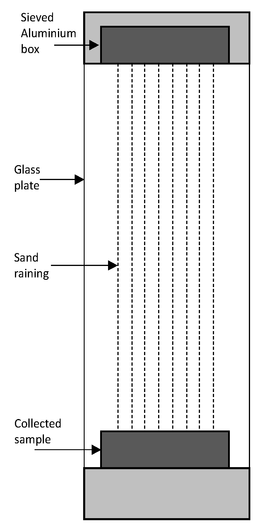
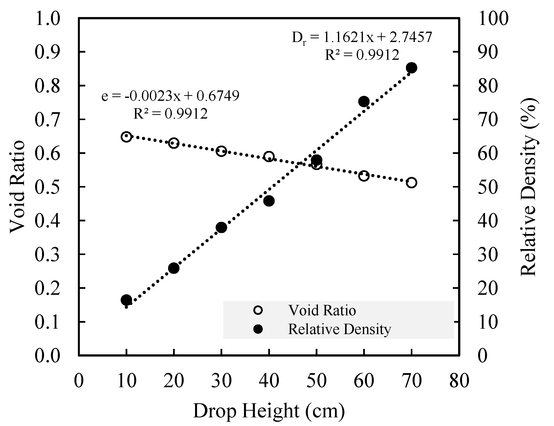
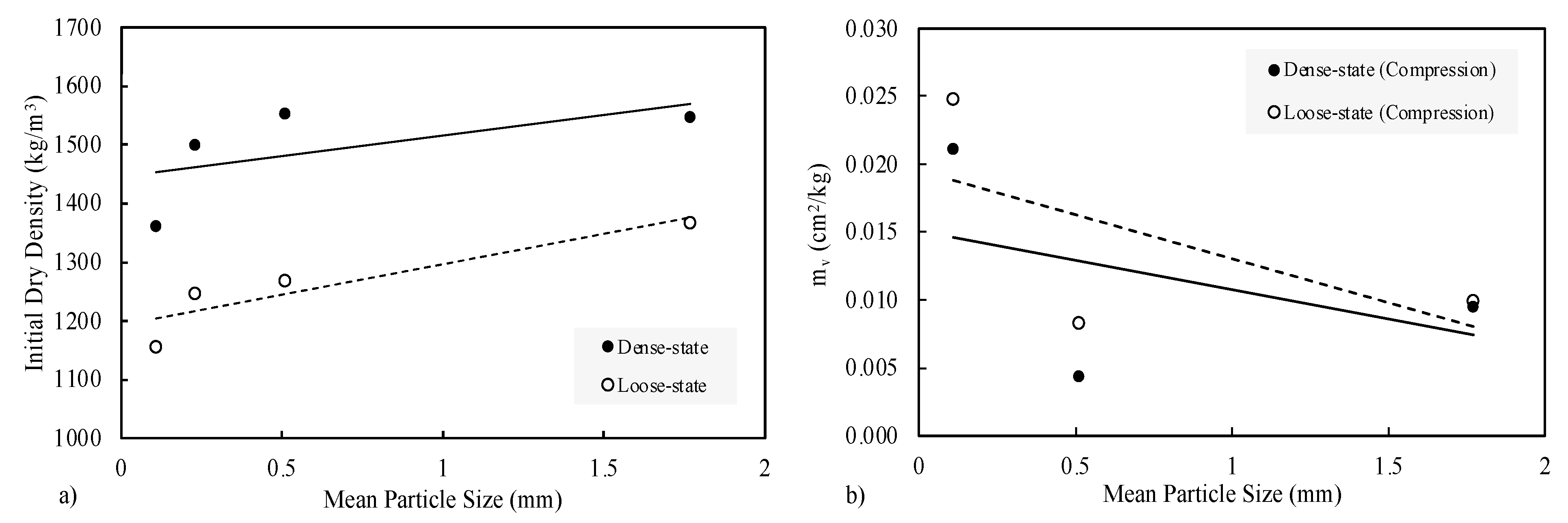
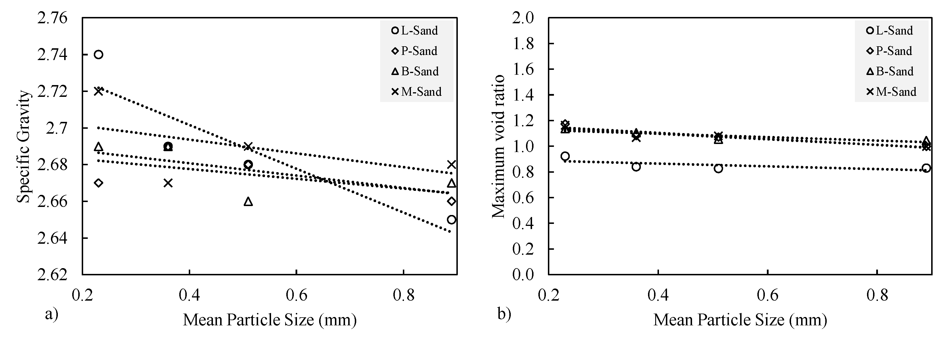
3.1.1. Packing Density

The structure of a sand sample (skeleton) plays a crucial role in determining the mechanical behaviour, which can be controlled by density and anisotropy. The packing density of sand can depend on multiple factors, such as the particle shape, size, and gradation along with the arrangement of particles. A sample consisting of particles with high regularity has a higher density and low void ratio compared to a sample with low regularity particles [2].
Sand gradation can be poorly graded, well graded, or gap graded. A poorly graded sand represents sand that has similar grain sizes; in contrast, the well-graded sand has a percentage of each size when the Cu is greater than 6 and when the Cc lies between 1 and 3. The gap-graded sand represents sand that has two different mixed sizes, in other words, two different poorly graded sands mixed together [9]. A well-graded sample will have a high density and a lower void ratio compared to a poorly graded sample.
According to Burmister [54], when the particle size range is coarser, the density increases and the void ratios decrease. In the poorly graded sand used, it was shown that as the mean particle size increases, the density also increases, and the coefficient of volume compressibility decreases, as demonstrated in Figure 8. These findings are consistent with the works of Burmister [54] and Lafata [1].
In terms of shape, there is a strong correlation between particle shape and packing density. A complete sphere shape has the densest possible structure compared to other shapes [1]. Spherical shapes require less compressive force to achieve a dense state because they are easier to reorient compared to less spherical shapes [1]. However, further studies [55] have shown that for particles of similar sizes, the optimal shape for achieving maximum packing fraction is not necessarily a perfect sphere. A comparison between a marble-ball model and M&M candies (which have an elongated and flattened shape) showed that the M&M candy shape has a higher packing fraction of C = 71% compared to a sphere shape with C = 64%. When examining the relationship between particle shape and void ratio, Cho, Dodds and Santamarina [2] found that as particle roundness, sphericity, and regularity approach one (indicating complete rounded and spherical shape), the difference between the maximum and minimum void ratio decreases. Similar results were found by Maroof et al. [56], where the void ratio decreased as regularity increased.
The mineral composition of a soil is one of its essential characteristics. Mineralogy influences properties such as specific gravity, Young’s modulus, shear modulus, and the Poisson ratio [12,57]. The dry unit weight and specific gravity of sand are important, as they can influence the sample’s void ratio, as shown in the following equation:
e = G s   γ w γ d 1
where Gs represents the specific gravity, γw indicates the unit weight of water, and γ d represents the dry unit weight of the sample. According to the equation, when the specific gravity increases, the void ratio also increases. Similarly, when the dry unit weight decreases, the void ratio increases. The specific gravity of sand typically ranges from 2.65–2.67, while that of inorganic clay ranges from 2.70–2.80 [58]. Based on the lab experiment, it was observed that among the four types of sand, as the D50 (mean particle size) of the sand increases, the dry unit weight of the sample also increases, while the specific gravity decreases, even within the range of sand particles (2.36 mm to 0.075 mm according to the Australian standard [7]). Consequently, the void ratio decreases as the mean particle size increases, as shown in Figure 9.

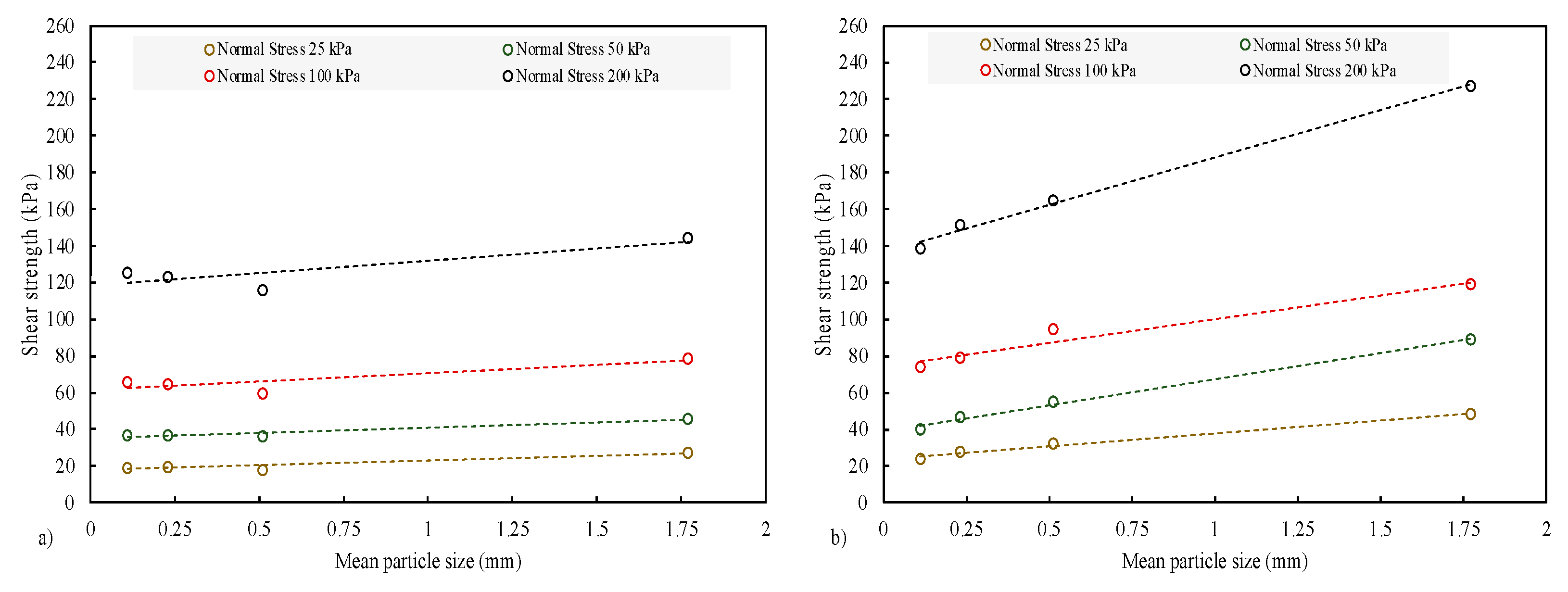
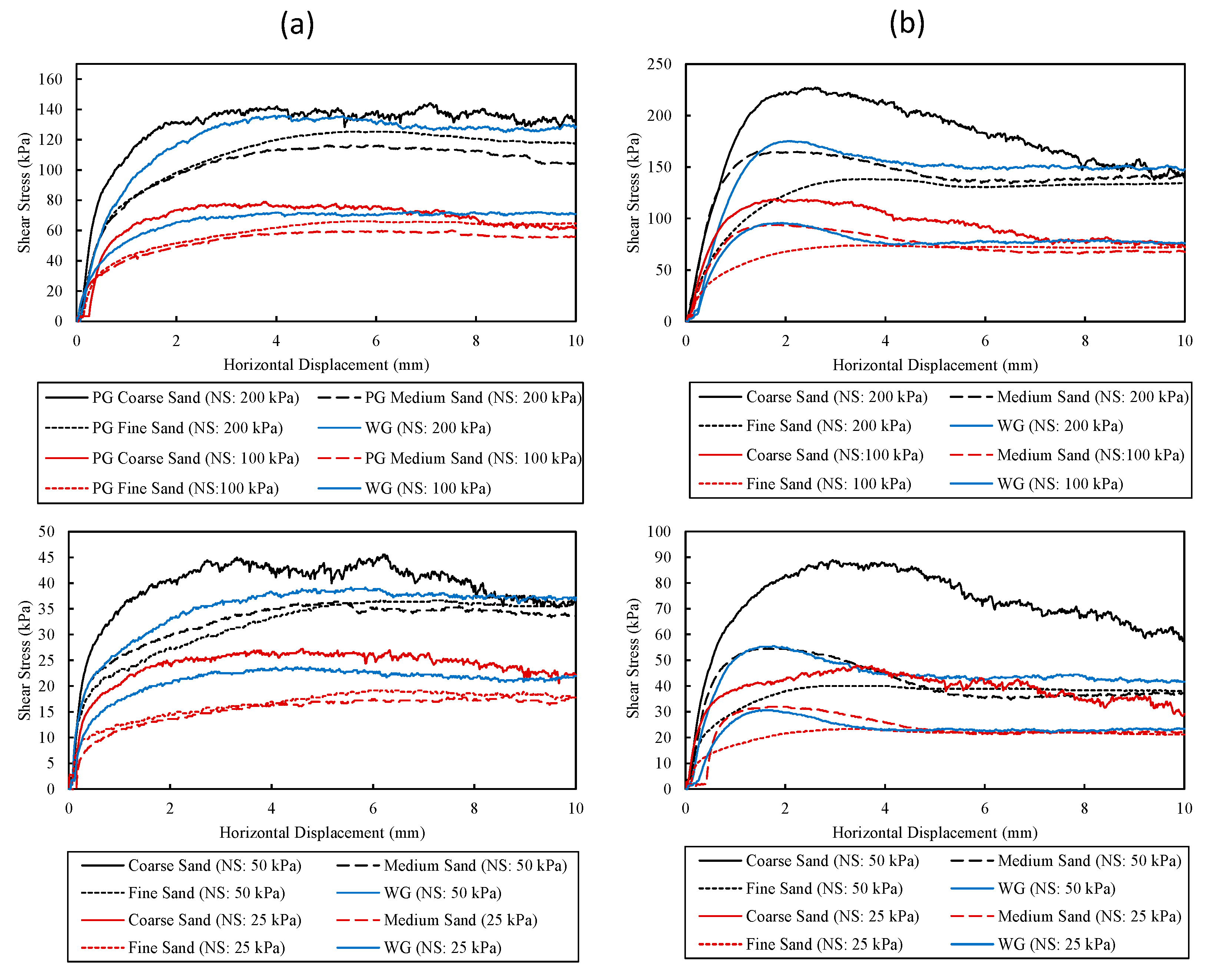
3.1.2. Shear Strength

The shear strength of the sand can depend on multiple factors related to the specimen, such as the particle shape, size, and gradation of the sand particles. Upon comparing the poorly graded fine, medium, and coarse sand, it was found that the coarse sand exhibited a higher shear strength compared to the others, as shown in Figure 10.
Furthermore, by examining the impact of gradation, the well-graded sand exhibits a higher density and shear strength when compared to fine and medium poorly graded sand, as shown in Figure 11. The well-graded sand had a higher shear strength value, though not as high as the coarse, poorly graded sand. This can be related to the particle shape, size, and surface roughness. Coarse sand particles, particularly those that are angular, can achieve higher shear strength due to particle interlocking. Furthermore, particles with high surface roughness can induce even greater shear strength due to the interlocking of asperities between the particles.

3.2. Machine Learning Models

3.2.1. Multiple Linear Regression

After conducting multiple linear regression (MLR) analyses, the most suitable regression model was identified. The comparison between the predicted values generated by the MLR model for training, testing, and 10-fold CV data and the actual experimental values of shear strength in the direct shear tests is presented in Figure 12. Based on the findings, it can be concluded that the MLR model has a high level of accuracy.
The usage of an MLR model for the objective of predicting the shear strength of sand showed high accuracy, as shown by the varied metrics gathered from the training, testing, and 10-fold CV data (Table 4).
The training database included 36 observations, with an MAE of 8.31, RMSE of 11.87, RMSLE of 0.29, and R2 value of 0.95, indicating a high level of prediction accuracy. The model was then tested on a separate dataset consisting of 10 observations, where it demonstrated a slightly improved MAE of 7.67 and a reduced RMSE of 10.08, and an impressive decrease in RMSLE to 0.17, maintaining a high R2 value of 0.94. Furthermore, a 10-fold cross-validation (CV) was performed on all 46 observations, yielding an MAE of 9.28, RMSE of 13.57, and RMSLE of 0.35, along with an R2 of 0.93. The model performance across the training, testing, and cross-validation demonstrates its robust predictive capability for shear strength. This outcome promotes confidence in the predictive capability of the model and its applicability to new data. Thus, an empirical equation was generated to predict the shear strength of sand with high level of accuracy. The empirical equation is as follows:
τ = 15.57 + 7.28 × D 50 + 6.75 × C u 24.53 × C c + 53.90 × ρ d r y + 121.64 × σ n ( 36.45 × ρ r )
where D50 is the mean particle size, Cu is the coefficient of uniformity, Cc is the coefficient of curvature, ρ d r y represents the dry density, σ n is the normal stress, and ρ r refers to the sand particle shape regularity.

3.2.2. Random Forest Regression

The comparison between the actual values of shear strength in direct shear testing and the predicted values for training, testing, and 10-fold CV data produced by the RFR model is shown in Figure 13. Based on the results, it can be concluded that the RFR model is highly accurate.
The Python-based RFR model has demonstrated remarkable accuracy in predicting the shear strength of sand, as evidenced by the metrics calculated for the training, testing, and 10-fold CV data (Table 5).
The training database used contained 36 observations, with an MAE of 3.79, RMSE of 6.55, RMSLE of 0.07, and an impressive R2 value of 0.98, signifying an excellent fit of the model. In the testing phase, using a distinct database of 10 observations, the model demonstrated slightly higher MAE and RMSE values of 5.68 and 7.37, respectively. The RMSLE also slightly increased to 0.09, yet the R2 value remained high at 0.97, indicating strong prediction performance. A 10-fold CV performed on the complete dataset of 46 observations resulted in an MAE of 9.83, RMSE of 15.8, RMSLE of 0.19, and an R2 value of 0.90. Despite the slight increase in error values during cross-validation, the RFR model demonstrated robust and reliable performance in predicting shear strength. These metrics serve as evidence of the model’s outstanding predictive performance and its ability to deliver consistent results on new data.

4. Discussion

4.1. Particulate Shape and Size

Particle morphology can be identified at larger scales, such as that of the particle itself, as spherical, rounded, blocky, bulky, platy, elliptical, elongated, and so on. On a smaller scale, texture is essential because it reflects local roughness properties such as surface smoothness, roundness of edges and corners, and asperities. As shown in Figure 14, there is no direct correlation between particle size and particle shape.
Polydispersity, a key concept in materials science and chemistry, refers to the distribution of particles with varying sizes or masses within a sample. Unlike monodisperse systems, where all particles are of the same size, polydisperse systems are characterized by non-uniform particles. It significantly influences the physical properties and behaviour of materials like soil samples, polymers, and colloids [59]. A shear test was conducted on glass beads of two different sizes. Each sample had a monodisperse size. Despite both samples having the same shape regularity, valued at 1, it was observed that the larger beads, with a D50 value of 1.77, exhibited higher shear strength at normal stresses of 25, 50, and 100 kPa, as shown in Figure 15. This was in comparison to the finer beads, which had a D50 value of 0.89. Therefore, we can conclude that larger particles can induce higher shear strength compared to finer particles.

4.2. Active Lateral Earth Pressure

The effects of particle size, density, and confining pressure on the active lateral earth pressure within a uniform type of sand, sorted into different mean particle sizes, are explored in Figure 16. The active lateral earth pressure increases as the mean particulate size increases. This result is because larger particles will have a higher dry density than smaller particles, which will increase the lateral earth pressure. Also, the active lateral earth pressure increases equally with increasing sample density; this increase is most likely due to an increase in particle content, as the number of particles in compact samples is greater than in loose samples. Therefore, the active lateral earth pressure is greater for denser samples. A similar correlation exists between an increase in normal stress and an increase in active lateral earth pressure. This phenomenon is related to the increased force applied perpendicular to the soil particles, which increase the active lateral earth pressure. In conclusion, the study highlights the importance of mean particle size, density, and normal stress on the active lateral earth pressure, where the active lateral earth pressure increases as the particle size, density, and confining pressure increase.

4.3. Method Comparison

Multiple linear regression (MLR) is a widely used method in supervised learning, especially for understanding and predicting linear relationships between variables. Owing to its optimal modelling strategy within the linear causal category, MLR often outperforms other standard models [60]. The motivation for using MLR stems from its established reputation as a simple, traditional model. Its strength lies in its capacity to capture linear relationships effectively between multiple predictors (independent variables) and a single response (dependent variable), making it particularly appealing for data analysis [29]. Additionally, MLR can provide an empirical equation for calculating shear strength using multiple inputs, offering utility in geotechnical engineering applications and practices.
Despite these strengths, MLR has its limitations, including its inability to handle nonlinear correlations or complex interactions between input data and the target variable. In response to these limitations, random forest regression (RFR) was employed. This robust and versatile technique navigates these challenges, offering high prediction performance [61]. The RFR model is an ensemble of regression trees, building a large number of these trees before combining them for a final prediction [62]. Moreover, RFR provides insights into feature importance, thereby helping to unravel underlying relationships in the data.
A comparison of the results and performance of both models can offer valuable insights into their respective strengths and weaknesses. This allows for an evaluation of how well each model captures the underlying patterns in the dataset and a determination of which model yields better results.
Table 6 presents a comparative performance analysis of MLR and RFR models applied to training, testing, and 10-fold cross-validation datasets. When comparing MAE values, the RFR model shows superior performance, particularly with the training data, where it achieved an MAE of 3.79, compared to 8.31 with MLR. This trend of enhanced performance continues in the testing data, but not in the cross-validation, where MLR produced a slightly better MAE result. For RMSE and RMSLE, RFR consistently outperforms MLR across all datasets, but not in the cross-validation, where MLR outperformed RFR in RMSE. In terms of R2 values, which indicate the goodness of fit, RFR shows a slight edge in the training and testing data, but MLR secures a slightly higher value in the 10-fold cross-validation data. Despite some minor variances, both models demonstrate robust predictive capabilities, although RFR generally exhibits stronger performance, particularly on the training and testing datasets.

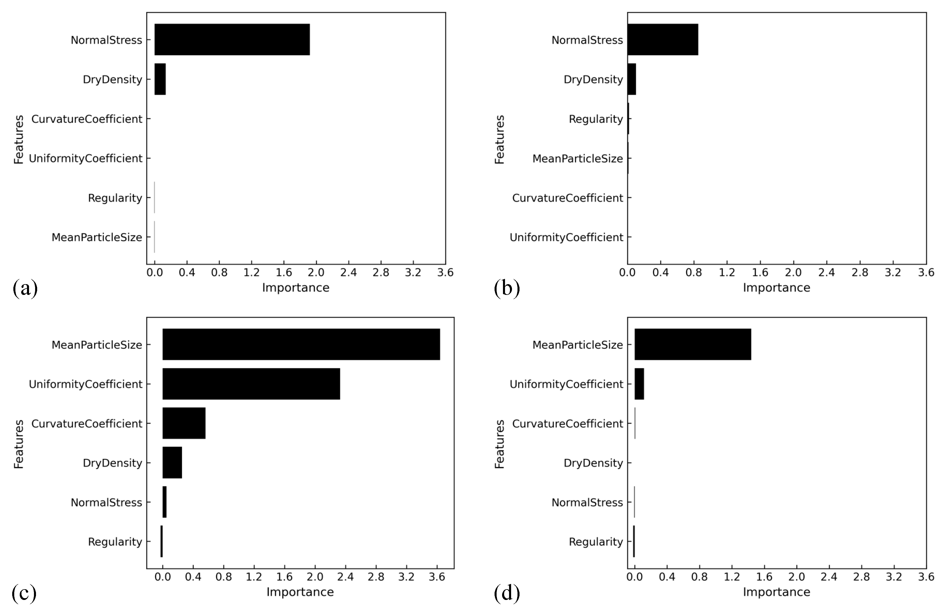
4.4. Importance of Features

The application of machine learning algorithms (MLR and RFR) in our study involves six input features (D50, Cu, Cc, Ꝭd, σn, r ) and one output which is the shear strength of sand. In Figure 17, both MLR and RFR models, when using the train test splits, identified normal stress as the principal factor, underlining its essential role in governing shear strength, while dry density followed as the second most influential parameter, highlighting its significance in determining the mass per unit volume. However, when using the 10-fold cross-validation method, mean particle size showed the highest feature importance, followed by coefficient of uniformity.

5. Conclusions

This study investigated the influence of sand particulate morphology on the shear strength characteristics using experimental and machine learning approaches. The findings can be summarized in the following points.
  • Across the range of poorly graded sand sizes, the large sand sample exhibits higher density and shear strength compared to both medium and fine sand.
  • The shear strength of well-graded sand is higher than that of poorly graded medium and fine sand, but not as high as that of poorly graded coarse sand.
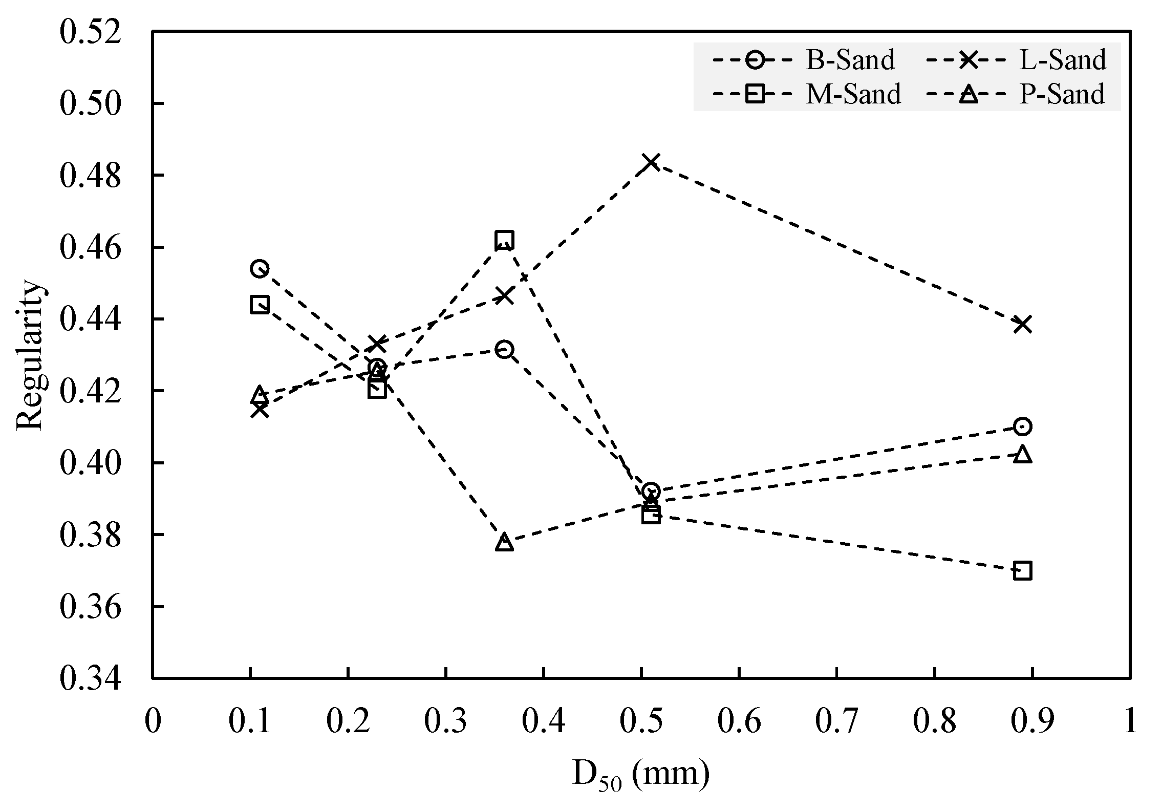
  • The particle shape regularity, including its roundness and sphericity, is not related to the mean particle size.
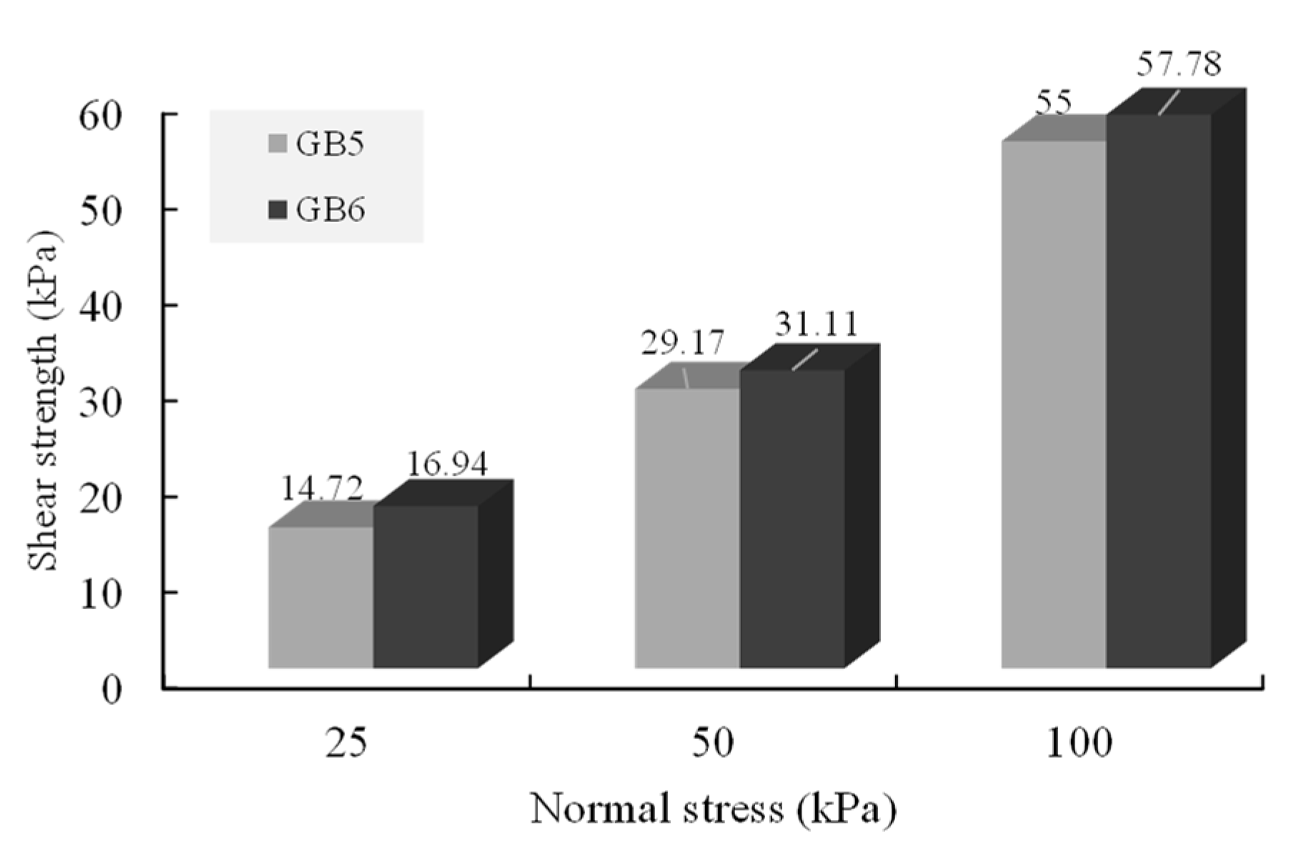
  • In a monodisperse system of glass beads with a similar shape and size, larger particles contribute to greater shear strength compared to their smaller counterparts.
  • As the mean particle size of sand decreases, the specific gravity increases and the density decreases, leading to a sample with a higher void ratio. Therefore, finer sand has a higher coefficient of volume compressibility compared to coarse sand.
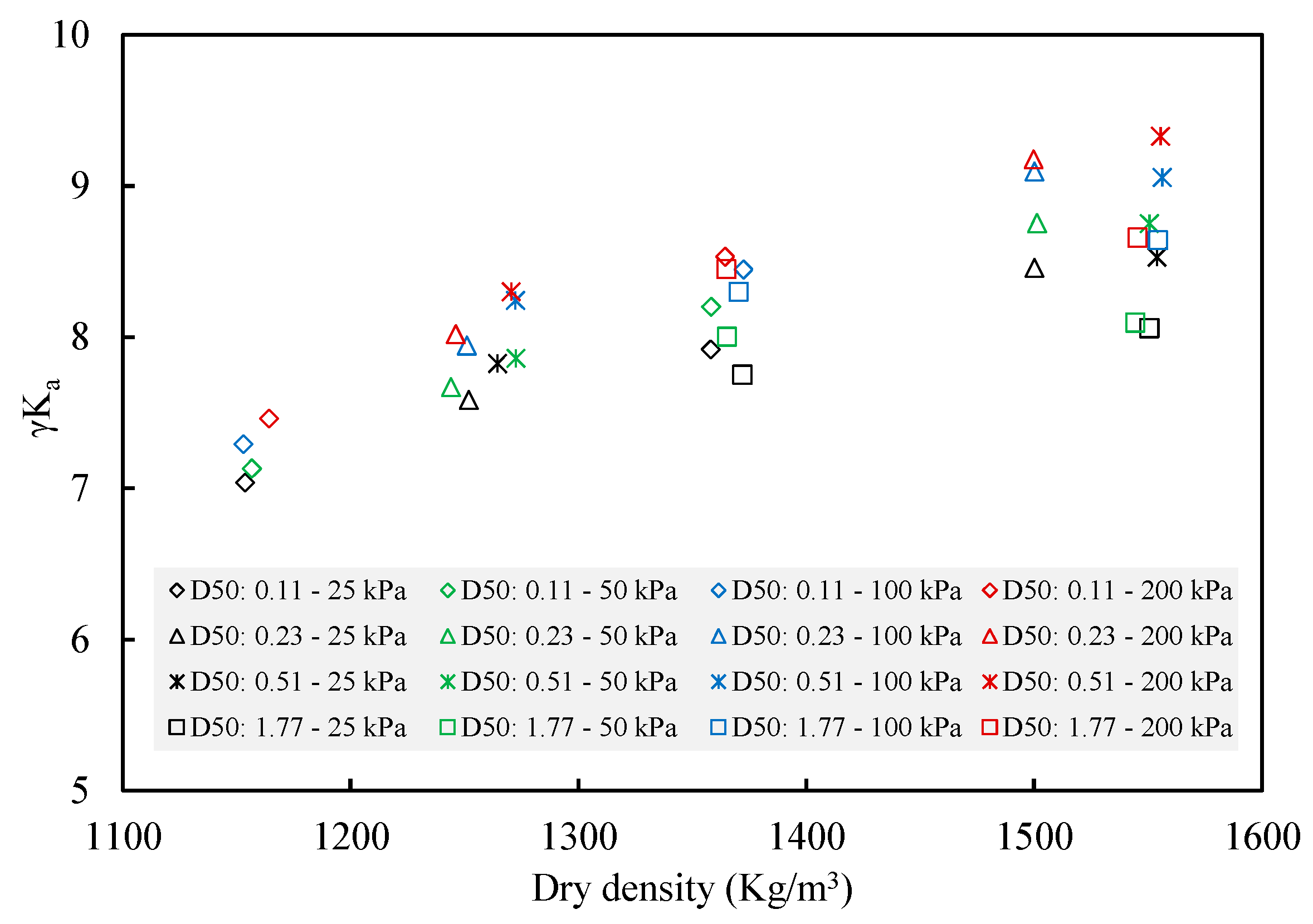
  • The active lateral earth pressure increases as the particle size, density, and confining pressure increases.
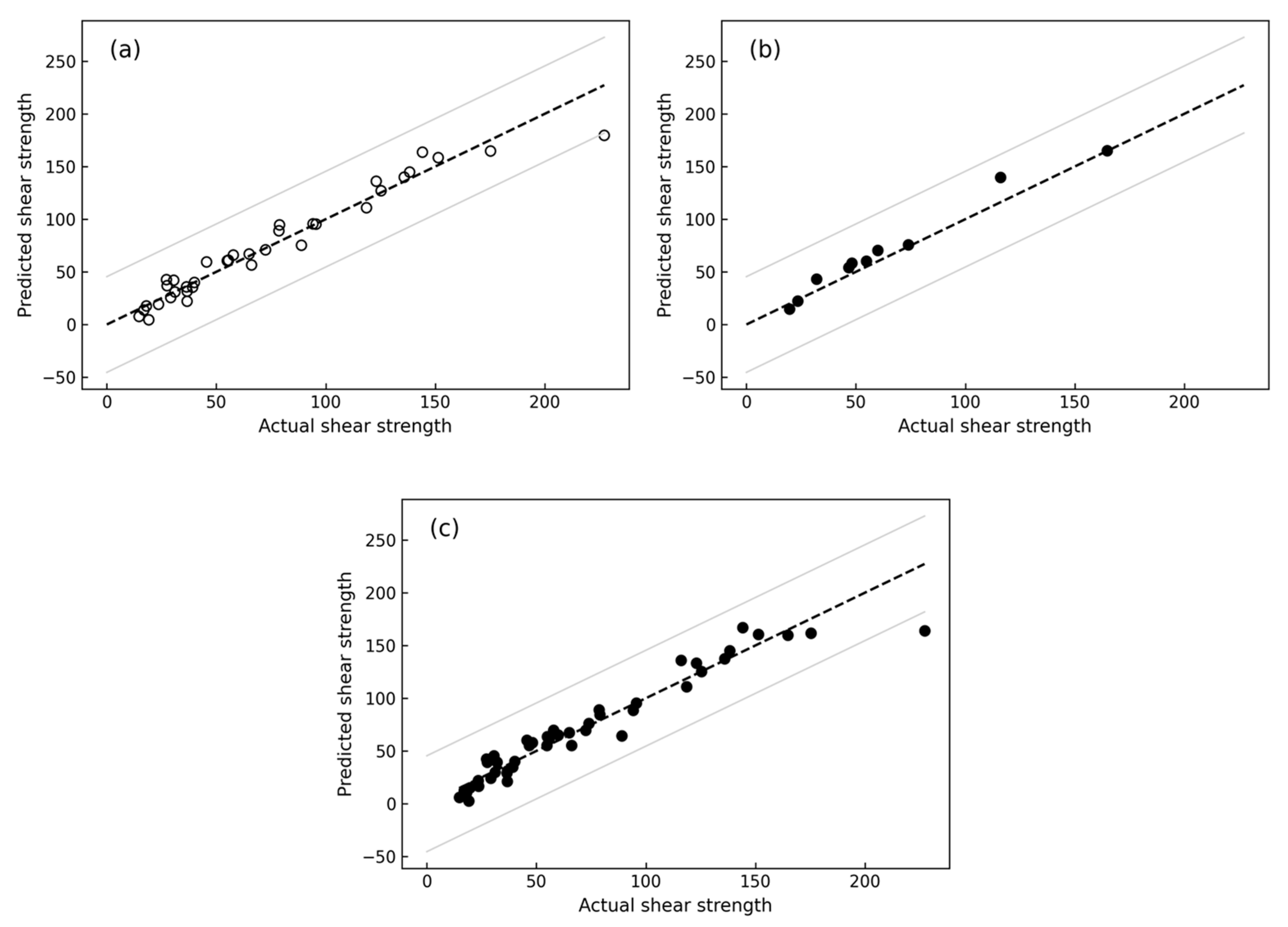
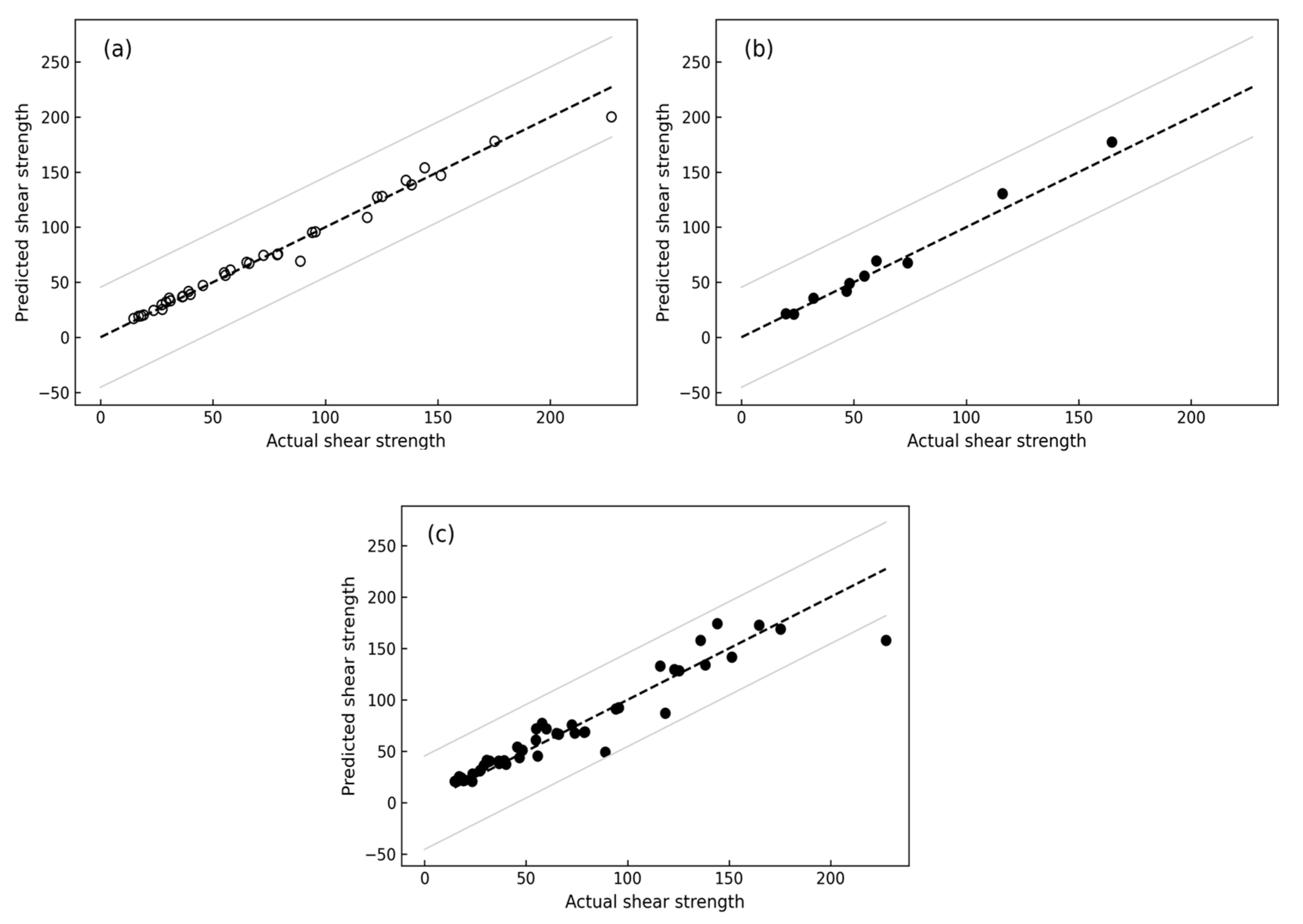
  • The machine learning models (MLR and RFR) show excellent accuracy in predicting the shear strength of sand based on different particle shapes, sizes, and gradations. In the case of MLR, the R-squared accuracy is 0.95 for the training data, 0.94 for the testing data, as well as 0.93 when using the entire dataset with 10-fold CV method. Similarly, for RFR, the R-squared accuracy is 0.98 for the training data, 0.97 for the testing data, and 0.90 when employing the entire dataset with the 10-fold CV method.
  • When using the train–test split, the machine learning models (MLR and RFR) agree on the importance of the following input features in sequence: normal stress and dry density. However, when using the 10-fold CV, the importance of the input features shifts to mean particle size and coefficient of uniformity.
  • Future research could address different types of soil (silt and clay), different parameters that could influence the shear strength (moisture content, temperature, strain rate, and stress history), as well as different machine learning algorithms for further exploration.

Author Contributions

Conceptualization, F.D. and H.A.-N.; methodology, F.D.; software, F.D.; writing—original draft preparation, F.D.; writing—review and editing, F.D. and H.A.-N.; supervision, H.A.-N. All authors have read and agreed to the published version of the manuscript.

Funding

The authors declare that no funds, grants, or other financial support were received during the preparation of this manuscript. This paper is part of the PhD of the first author.

Institutional Review Board Statement

Not applicable.

Informed Consent Statement

Not applicable.

Data Availability Statement

Not applicable.

Conflicts of Interest

The authors declare no conflict of interest.

Nomenclature

AI  Artificial Intelligence
MLR  Multiple Linear Regression
RFR  Random Forest Regression
ANN  Artificial Neural Network
SVM  Support Vector Machine
ANFIS  Adaptive Neuro-Fuzzy Inference System
ME  Mean Error
MAE  Mean Absolute Error
MSE  Mean Square Error
RMSE  Root Mean Square Error
RMSLE  Root Mean Square Log Error
CV  Cross-validation
R2  R-squared
D50  Mean Particle Size
Cu  Coefficient of Uniformity
Cc  Coefficient of Curvature
d  Dry Density
σn  Normal Stress
R  Roundness
S  Sphericity
r   Particle Regularity
Dr  Relative Density
e  Void ratio
emin  Minimum Void Ratio
emax  Maximum Void Ratio
Gs  Specific Gravity
γw   Unit Weight of Water
γ d   Dry Unit Weight of The Sample
τ   Shear Strength
SOC  Soil Organic Carbon

References

  1. Lafata, L. Effect of Particle Shape and Size on Compressibility Behavior of Dredged Sediment in a Geotextile Tube Dewatering Application. 2014. Available online: https://surface.syr.edu/honors_capstone/757/ (accessed on 3 January 2023).
  2. Cho, G.-C.; Dodds, J.; Santamarina, J.C. Particle shape effects on packing density, stiffness, and strength: Natural and crushed sands. J. Geotech. Geoenviron. 2006, 132, 591–602. [Google Scholar] [CrossRef] [Green Version]
  3. Frost, J.; Han, J. Behavior of interfaces between fiber-reinforced polymers and sands. J. Geotech. Geoenviron. Eng. 1999, 125, 633–640. [Google Scholar] [CrossRef]
  4. Shaia, H. Behaviour of Fibre Reinforced Polymer Composite Piles: Experimental and Numerical Study; The University of Manchester: Manchester, UK, 2013. [Google Scholar]
  5. Su, L.-J.; Zhou, W.-H.; Chen, W.-B.; Jie, X. Effects of relative roughness and mean particle size on the shear strength of sand-steel interface. Measurement 2018, 122, 339–346. [Google Scholar] [CrossRef]
  6. Vaid, Y.; Rinne, N. Geomembrane coefficients of interface friction. Geosynth. Int. 1995, 2, 309–325. [Google Scholar] [CrossRef]
  7. AS1289.3.6.1; Method of Testing Soils for Engineering Purposes—Soil Classification. Australian Standard: Sydney, NSW, Australia, 2009.
  8. Barrett, P. The shape of rock particles, a critical review. Sedimentology 1980, 27, 291–303. [Google Scholar] [CrossRef]
  9. Das, B.M. Principles of Geotehcnical Engineering; Cengage Learning: Boston, MA, USA, 2010. [Google Scholar]
  10. Sarkar, D. Influence of Particle Characteristics on the Behaviour of Granular Materials under Static, Cyclic and Dynamic Loading. 2023. Available online: https://www.researchgate.net/profile/Debdeep-Sarkar/publication/370265264_Influence_of_particle_characteristics_on_the_behaviour_of_granular_materials_under_static_cyclic_and_dynamic_loading/links/6448dc28d749e4340e389659/Influence-of-particle-characteristics-on-the-behaviour-of-granular-materials-under-static-cyclic-and-dynamic-loading.pdf (accessed on 3 January 2023).
  11. Dodds, J.S. Particle Shape and Stiffness: Effects on Soil Behavior; Civil and Environmental Engineering, Georgia Institute of Technology: Atlanta, GA, USA, 2003. [Google Scholar]
  12. Mitchell, J.K.; Soga, K. Fundamentals of Soil Behavior; John Wiley & Sons: New York, NY, USA, 2005; Volume 3. [Google Scholar]
  13. Wadell, H. Volume, shape, and roundness of rock particles. J. Geol. 1932, 40, 443–451. [Google Scholar] [CrossRef]
  14. Powers, M.C. A new roundness scale for sedimentary particles. J. Sediment. Res. 1953, 23, 117–119. [Google Scholar] [CrossRef]
  15. Schanz, T.; Vermeer, P. Angles of friction and dilatancy of sand. Géotechnique 1996, 46, 145–151. [Google Scholar] [CrossRef] [Green Version]
  16. Li, Y. Effects of particle shape and size distribution on the shear strength behavior of composite soils. Bull. Eng. Geol. Environ. 2013, 72, 371–381. [Google Scholar] [CrossRef]
  17. Peng, Z.; Chen, C.; Wu, L. Numerical investigation of particle shape effect on sand shear strength. Arab. J. Sci. Eng. 2021, 46, 10585–10595. [Google Scholar] [CrossRef]
  18. Otsubo, M.; O’sullivan, C.; Sim, W.W.; Ibraim, E. Quantitative assessment of the influence of surface roughness on soil stiffness. Géotechnique 2015, 65, 694–700. [Google Scholar] [CrossRef] [Green Version]
  19. Santamarina, C.; Cascante, G. Effect of surface roughness on wave propagation parameters. Geotechnique 1998, 48, 129–136. [Google Scholar] [CrossRef]
  20. Tsomokos, A.; Georgiannou, V. Effect of grain shape and angularity on the undrained response of fine sands. Can. Geotech. J. 2010, 47, 539–551. [Google Scholar] [CrossRef]
  21. Menq, F.; Stokoe, K. Linear dynamic properties of sandy and gravelly soils from large-scale resonant tests. In Proceedings of the Deformation Characteristics of Geomaterials, IS Lyon 2003, Lyon, France, 22–24 September 2003; pp. 63–71. [Google Scholar]
  22. Miura, K.; Maeda, K.; Furukawa, M.; Toki, S. Physical characteristics of sands with different primary properties. Soils Found. 1997, 37, 53–64. [Google Scholar] [CrossRef] [Green Version]
  23. Vangla, P.; Latha, G.M. Influence of particle size on the friction and interfacial shear strength of sands of similar morphology. Int. J. Geosynth. Ground Eng. 2015, 1, 6. [Google Scholar] [CrossRef] [Green Version]
  24. Wang, J.-J.; Zhang, H.-P.; Tang, S.-C.; Liang, Y. Effects of particle size distribution on shear strength of accumulation soil. J. Geotech. Geoenviron. Eng. 2013, 139, 1994–1997. [Google Scholar] [CrossRef]
  25. Islam, M.N.; Siddika, A.; Hossain, M.B.; Rahman, A.; Asad, M.A. Effect of particle size on the shear strength behavior of sands. arXiv 2019, arXiv:1902.09079. [Google Scholar]
  26. Alias, R.; Kasa, A.; Taha, M. Particle size effect on shear strength of granular materials in direct shear test. Int. J. Civ. Environ. Eng. 2014, 8, 1144–1147. [Google Scholar]
  27. Skinner, A. A note on the influence of interparticle friction on the shearing strength of a random assembly of spherical particles. Geotechnique 1969, 19, 150–157. [Google Scholar] [CrossRef]
  28. Xie, X.; Wu, T.; Zhu, M.; Jiang, G.; Xu, Y.; Wang, X.; Pu, L. Comparison of random forest and multiple linear regression models for estimation of soil extracellular enzyme activities in agricultural reclaimed coastal saline land. Ecol. Indic. 2021, 120, 106925. [Google Scholar] [CrossRef]
  29. Zhang, H.; Wu, P.; Yin, A.; Yang, X.; Zhang, M.; Gao, C. Prediction of soil organic carbon in an intensively managed reclamation zone of eastern China: A comparison of multiple linear regressions and the random forest model. Sci. Total Environ. 2017, 592, 704–713. [Google Scholar] [CrossRef] [PubMed]
  30. Jang, J.-S. ANFIS: Adaptive-network-based fuzzy inference system. IEEE Trans. Syst. Man Cybern. 1993, 23, 665–685. [Google Scholar] [CrossRef]
  31. Keshwani, D.R.; Jones, D.D.; Brand, R.M. Takagi–Sugeno Fuzzy Modeling of Skin Permeability. Cutan. Ocul. Toxicol. 2005, 24, 149–163. [Google Scholar] [CrossRef] [PubMed]
  32. Al-Mahasneh, M.; Aljarrah, M.; Rababah, T.; Alu’datt, M. Application of hybrid neural fuzzy system (ANFIS) in food processing and technology. Food Eng. Rev. 2016, 8, 351–366. [Google Scholar] [CrossRef]
  33. Sonmez, A.Y.; Kale, S.; Ozdemir, R.C.; Kadak, A.E. An adaptive neuro-fuzzy inference system (ANFIS) to predict of cadmium (Cd) concentrations in the Filyos River, Turkey. Turk. J. Fish. Aquat. Sci. 2018, 18, 1333–1343. [Google Scholar] [CrossRef] [PubMed]
  34. Bensaber, B.A.; Diaz, C.G.P.; Lahrouni, Y. Design and modeling an Adaptive Neuro-Fuzzy Inference System (ANFIS) for the prediction of a security index in VANET. J. Comput. Sci. 2020, 47, 101234. [Google Scholar] [CrossRef]
  35. Akkaya, E. ANFIS based prediction model for biomass heating value using proximate analysis components. Fuel 2016, 180, 687–693. [Google Scholar] [CrossRef]
  36. Abdulshahed, A.M.; Longstaff, A.P.; Fletcher, S. The application of ANFIS prediction models for thermal error compensation on CNC machine tools. Appl. Soft Comput. 2015, 27, 158–168. [Google Scholar] [CrossRef]
  37. Hsieh, M.-C.; Maurya, S.N.; Luo, W.-J.; Li, K.-Y.; Hao, L.; Bhuyar, P. Coolant Volume Prediction for Spindle Cooler with Adaptive Neuro-fuzzy Inference System Control Method. Sens. Mater. 2022, 34, 2447–2466. [Google Scholar] [CrossRef]
  38. Bardhan, A.; Samui, P. Application of artificial intelligence techniques in slope stability analysis: A short review and future prospects. Int. J. Geotech. Earthq. Eng. (IJGEE) 2022, 13, 1–22. [Google Scholar] [CrossRef]
  39. Inazumi, S.; Intui, S.; Jotisankasa, A.; Chaiprakaikeow, S.; Kojima, K. Artificial intelligence system for supporting soil classification. Results Eng. 2020, 8, 100188. [Google Scholar] [CrossRef]
  40. Singh, B.; Sihag, P.; Pandhiani, S.M.; Debnath, S.; Gautam, S. Estimation of permeability of soil using easy measured soil parameters: Assessing the artificial intelligence-based models. ISH J. Hydraul. Eng. 2021, 27, 38–48. [Google Scholar] [CrossRef]
  41. Baghbani, A.; Costa, S.; Choundhury, T.; Faradonbeh, R.S. Prediction of Parallel Desiccation Cracks of Clays Using a Classification and Regression Tree (CART) Technique. In Proceedings of the 8th International Symposium on Geotechnical Safety and Risk (ISGSR), Newcastle, Australia, 14–16 December 2022. [Google Scholar]
  42. Daghistani, F.; Baghbani, A.; Abuel Naga, H.; Faradonbeh, R.S. Internal Friction Angle of Cohesionless Binary Mixture Sand–Granular Rubber Using Experimental Study and Machine Learning. Geosciences 2023, 13, 197. [Google Scholar] [CrossRef]
  43. Baghbani, A.; Daghistani, F.; Baghbani, H.; Kiany, K. Predicting the Strength of Recycled Glass Powder-Based Geopolymers for Improving Mechanical Behavior of Clay Soils Using Artificial Intelligence; EasyChair: Manchester, UK, 2023. [Google Scholar]
  44. Baghbani, A.; Daghistani, F.; Kiany, K.; Shalchiyan, M.M. AI-Based Prediction of Strength and Tensile Properties of Expansive Soil Stabilized with Recycled Ash and Natural Fibers; EasyChair: Manchester, UK, 2023. [Google Scholar]
  45. Baghbani, A.; Daghistani, F.; Baghbani, H.; Kiany, K.; Bazaz, J.B. Artificial Intelligence-Based Prediction of Geotechnical Impacts of Polyethylene Bottles and Polypropylene on Clayey Soil; EasyChair: Manchester, UK, 2023. [Google Scholar]
  46. Baghbani, A.; Daghistani, F.; Naga, H.A.; Costa, S. Development of a Support Vector Machine (SVM) and a Classification and Regression Tree (CART) to Predict the Shear Strength of Sand Rubber Mixtures. In Proceedings of the 8th International Symposium on Geotechnical Safety and Risk (ISGSR), Newcastle, Australia, 14–16 December 2022. [Google Scholar]
  47. AS1774.19; The Determination of Sieve Analysis and Moisture Content. Australian Standard: Sydney, NSW, Australia, 2003.
  48. AS1289.6.2.2; Soil Strength and Consolidation Tests—Determination of Shear Strength of a Soil—Direct Shear Test Using a Shear Box. Australian Standard: Sydney, NSW, Australia, 2020.
  49. Krumbein, W.; Sloss, L. Stratigraphy and Sedimentation, 2nd ed.; Friedman, WH and Company: San Francisco, CA, USA, 1963; Volume 660. [Google Scholar]
  50. Liu, Y.-L.; Nisa, E.C.; Kuan, Y.-D.; Luo, W.-J.; Feng, C.-C. Combining deep neural network with genetic algorithm for axial flow fan design and development. Processes 2023, 11, 122. [Google Scholar] [CrossRef]
  51. Joseph, V.R. Optimal ratio for data splitting. Stat. Anal. Data Min. ASA Data Sci. J. 2022, 15, 531–538. [Google Scholar] [CrossRef]
  52. Vakharia, V.; Shah, M.; Nair, P.; Borade, H.; Sahlot, P.; Wankhede, V. Estimation of Lithium-ion Battery Discharge Capacity by Integrating Optimized Explainable-AI and Stacked LSTM Model. Batteries 2023, 9, 125. [Google Scholar] [CrossRef]
  53. Rochman, E.; Rachmad, A.; Fatah, D.; Setiawan, W.; Kustiyahningsih, Y. Classification of Salt Quality based on Salt-Forming Composition using Random Forest. J. Phys. Conf. Ser. 2022, 2406, 012021. [Google Scholar] [CrossRef]
  54. Burmister, D.M. Study of the Physical Characteristics of Soils, with Special Reference to Earth Structures; Department of Civil Engineering Columbia University: New York, NY, USA, 1938. [Google Scholar]
  55. Guyon, E.; Delenne, J.Y.; Radjai, F.; Kamrin, K.; Butler, E. Built on Sand: The Science of Granular Materials; MIT Press: Cambridge, MA, USA, 2020. [Google Scholar]
  56. Maroof, M.A.; Mahboubi, A.; Vincens, E.; Noorzad, A. Effects of particle morphology on the minimum and maximum void ratios of granular materials. Granul. Matter 2022, 24, 1–24. [Google Scholar] [CrossRef]
  57. Terzaghi, K.; Peck, R.B.; Mesri, G. Soil Mechanics in Engineering Practice; John Wiley & Sons: Hoboken, NJ, USA, 1996. [Google Scholar]
  58. Bowles, J.E. Engineering Properties of Soils and Their Measurement; McGraw-Hill, Inc.: New York, NY, USA, 1992. [Google Scholar]
  59. Voivret, C.; Radjai, F.; Delenne, J.-Y.; El Youssoufi, M.S. Space-filling properties of polydisperse granular media. Phys. Rev. E 2007, 76, 021301. [Google Scholar] [CrossRef]
  60. Etemadi, S.; Khashei, M. Etemadi multiple linear regression. Measurement 2021, 186, 110080. [Google Scholar] [CrossRef]
  61. Breiman, L. Random forests. Mach. Learn. 2001, 45, 5–32. [Google Scholar] [CrossRef] [Green Version]
  62. Pahlavan-Rad, M.R.; Dahmardeh, K.; Hadizadeh, M.; Keykha, G.; Mohammadnia, N.; Gangali, M.; Keikha, M.; Davatgar, N.; Brungard, C. Prediction of soil water infiltration using multiple linear regression and random forest in a dry flood plain, eastern Iran. Catena 2020, 194, 104715. [Google Scholar] [CrossRef]
Figure 1. The coarse soil (B-sand) is sieved and separated into different containers depending on the granular size.
Applsci 13 08160 g001
Figure 2. Sieve analysis of the used particulate materials, with (a) displaying the sieve analysis for sand, and (b) showing the sieve analysis for glass beads.
Applsci 13 08160 g002
Figure 3. Schematic view of the pluviation technique.
Applsci 13 08160 g003
Figure 4. Drop height versus void ratio and relative density of L-Sand.
Applsci 13 08160 g004
Figure 5. Determining particle shape through sphericity and roundness, with diagonal dotted lines indicating consistent particle regularity r = ( R + S ) 2 [2,49].
Applsci 13 08160 g005
Figure 6. Schematic illustration of determining the particle shape parameters: roundness, sphericity, and regularity.
Applsci 13 08160 g006
Figure 7. Workflow of the applied machine learning algorithm.
Applsci 13 08160 g007
Figure 8. The relationship between the mean particle size and (a) initial dry density and (b) coefficient of volume compressibility.
Applsci 13 08160 g008
Figure 9. The mean particle sizes of different sands in relation to (a) specific gravity and (b) maximum void ratio.
Applsci 13 08160 g009
Figure 10. Shear strength versus mean particle size for B-Sand in (a) a loose density state and (b) a dense density state.
Applsci 13 08160 g010
Figure 11. The particle size and gradation impact on the shear strength at different normal stresses (25, 50, 100, and 200) at different densities: (a) loose state, and (b) dense state.
Applsci 13 08160 g011
Figure 12. Multiple linear regression was performed to compare actual shear strength with predicted shear strength using (a) the training database, (b) the testing database, and (c) 10-fold cross-validation.
Applsci 13 08160 g012
Figure 13. Random forest regression was performed to compare actual shear strength with predicted shear strength using (a) the training database, (b) the testing database, and (c) 10-fold cross-validation.
Applsci 13 08160 g013
Figure 14. Mean particle size versus the regularity.
Applsci 13 08160 g014
Figure 15. Shear strength versus normal stress for two different mean particle sizes of glass beads.
Applsci 13 08160 g015
Figure 16. Comparison of active lateral earth pressure and dry density for different particle sizes of various sands under different normal stresses.
Applsci 13 08160 g016
Figure 17. Feature importance analysis comparing multiple linear regression and random forest regression with and without 10-fold cross-validation: (a) MLR without 10-fold cross-validation, (b) RFR without 10-fold cross-validation, (c) MLR with 10-fold cross-validation, (d) RFR with 10-fold cross-validation.
Applsci 13 08160 g017
Table 1. Specifications of the used particulate materials: sand and glass beads.
MaterialRange (mm)GradeCuCcD50 (mm)GsRS r
L5-Sand1.18 to 0.6PG 11.440.960.892.650.2880.5890.439
L4-Sand0.6 to 0.425PG1.200.970.512.680.4210.5460.484
L3-Sand0.425 to 0.3PG1.200.970.362.690.3020.5910.447
L2-Sand0.3 to 0.15PG1.450.960.232.740.2880.5780.433
L1-Sand0.15 to 0.075PG1.450.960.11-0.2890.5410.415
B-Sand2.36 to 0.075WG 26.161.240.582.67---
B6-Sand2.36 to 1.18PG1.450.961.772.66---
B5-Sand1.18 to 0.6PG1.440.960.892.670.2630.5570.410
B4-Sand0.6 to 0.425PG1.200.970.512.660.2460.5380.392
B3-Sand0.425 to 0.3PG1.200.970.362.690.2790.5840.432
B2-Sand0.3 to 0.15PG1.450.960.232.690.2700.5830.427
B1-Sand0.15 to 0.075PG1.450.960.112.700.3280.5800.454
M5-Sand1.18 to 0.6PG1.440.960.892.680.1890.5510.370
M4-Sand0.6 to 0.425PG1.200.970.512.690.2060.5650.386
M3-Sand0.425 to 0.3PG1.200.970.362.670.3270.5970.462
M2-Sand0.3 to 0.15PG1.450.960.232.720.2990.5420.421
M1-Sand0.15 to 0.075PG1.450.960.11-0.3890.4990.444
P5-Sand1.18 to 0.6PG1.440.960.892.660.2460.5590.403
P4-Sand0.6 to 0.425PG1.200.970.512.680.2030.5750.389
P3-Sand0.425 to 0.3PG1.200.970.362.690.2330.5230.378
P2-Sand0.3 to 0.15PG1.450.960.232.670.2860.5650.426
P1-Sand0.15 to 0.075PG1.450.960.11-0.3300.5080.419
GB6 *2.36 to 1.18PG1.450.961.772.45111
GB51.18 to 0.6PG1.440.960.892.45111
* Where GB is glass beads, 1 PG is poorly graded, and 2 WG is well graded sand.
Table 2. Numerical hyperparameters for the multiple linear regression code, including parameters for both with and without the application of 10-fold CV.
PhaseParameterValue
Train and Test Setstest_size0.2
random_state0
K-Fold Cross-Validationn_splits10
random_state0
shuffleTrue
Feature Importance Estimationn_repeats10
Visualisationstart_point0
boundary_shift20%
Table 3. Numerical hyperparameters for the random forest regressor code, including parameters for both with and without the application of 10-fold CV.
PhaseParameterValue
Train and Test Setstest_size0.2
random_state0
K-Fold Cross-Validationn_splits10
random_state0
shuffleTrue
Modeln_estimators100
random_state0
Visualisationstart_point0
boundary_shift20%
Table 4. The performance of MLR model to predict shear strength.
Training DatabaseTesting Database10-Fold CV
Observations361046
MAE8.317.679.28
RMSE11.8710.0813.57
RMSLE0.290.170.35
R20.950.940.93
Table 5. The performance of RFR to predict shear strength.
Training DatabaseTesting Database10-Fold CV
Observations361046
MAE3.795.689.83
RMSE6.557.3715.8
RMSLE0.070.090.19
R20.980.970.90
Table 6. Comparative performance of multiple linear regression and random forest regression on training, testing, and 10-fold cross-validation datasets.
Performance
Metrics
MLRRFR
Training DataTesting Data10-Fold CVTraining DataTesting Data10-Fold CV
MAE8.317.679.283.795.689.83
RMSE11.8710.0813.576.557.3715.8
RMSLE0.290.170.350.070.090.19
R20.950.940.930.980.970.90
Disclaimer/Publisher’s Note: The statements, opinions and data contained in all publications are solely those of the individual author(s) and contributor(s) and not of MDPI and/or the editor(s). MDPI and/or the editor(s) disclaim responsibility for any injury to people or property resulting from any ideas, methods, instructions or products referred to in the content.

