Intelligent Machinery Fault Diagnosis Method Based on Adaptive Deep Convolutional Neural Network: Using Dental Milling Cutter Malfunction Classifications as an Example

Abstract

Intelligent machinery fault diagnosis is one of the key technologies for the transformation and competitiveness of traditional factories. Complex production environments make it difficult to maintain good prediction performance using traditional methods. This paper proposes a deep convolutional neural network combined with an adaptive environmental noise method to achieve robust fault classification. The proposed method uses six-dimensional physical signals for data fusion and feature fusion, extracts obvious features and enhances subtle features, and uses continuous wavelets and Gramian angular fields to transform signals with different physical and frequency characteristics into time–frequency maps and two-dimensional images. The fusion technology of different signals can provide comprehensive features for fault prediction, improving upon the blind spots of traditional methods to extract features, and then perform prediction and classification through deep convolutional neural networks. In the experiment, the tool failure classification of the dental milling machine is used as a verification case. The results show that the prediction accuracy of the proposed method is nearly 100%, much better than other comparison methods. In addition, white noise was added in the experiment to verify the noise immunity of the model. The results show that the accuracy of the proposed method is 99%, which is better than other comparison methods in terms of accuracy and robustness, proving the effectiveness of the proposed method for fault diagnosis and classification.

1. Introduction

The demand for dentures continually increases year after year. Since 2001, the global compound annual growth rate of the dental implant market has been around 17.7%. Problems such as cutter wear during the creation of dentures can result in missing edges and decreased accuracy, rendering the product defective and unusable. At present, the only way the quality of the cutter is determined is through the traditional calculation of the number of finished products, making it difficult to reduce costs or improve production quality. Additionally, overheating caused by excessive tool wear and dull blades often causes the tool to tip or even break. Therefore, a key technology for upgrading the current denture processing is an intelligent prediction method of the quality of the tool.

As modern industries shift towards artificial intelligence, an important research direction is predicting and diagnosing malfunctions in intelligent machinery. Mechanical malfunctions tend to be small and hard to detect. When these failures occur, it often causes equipment shutdown or damage, which indirectly causes economic losses or casualties. Therefore, an important core technology of smart machinery is how to improve equipment activation through intelligent sensing and fault diagnosis prediction, and how to reduce the risk of downtime due to equipment failure. There are many types of mechanical equipment failures, such as abrasion and damage of the processing machine’s spindle cutter [1,2,3,4,5,6,7], the abnormal damage of the bearing [8,9,10,11,12] or gearbox of the rotary machinery due to the harsh environment, rotational instability caused by mechanical failures of the power generator, etc. Therefore, accurate prediction of mechanical failures will reduce production losses, a key factor, and condition for the efficient production of smart machinery.

Intelligent machinery fault diagnosis is divided into five steps, namely: (1) data collection; (2) data preprocessing; (3) feature extraction; (4) model training; and (5) fault classification. Data-driven intelligent sensing not only relies upon accurate data acquisition and data preprocessing, but feature extraction is also a major factor. In practice, sensory data are affected by noise in harsh production environments, and redundant information reduces the accuracy of model predictions. The sensory data captured by mechanical fault diagnosis includes vibration, noise, currents, temperature, cutting force and rotational speed, and so forth. Different sensors have different sensitivities and characteristic modes for fault diagnosis, making it difficult to use a single sensing data to improve the accuracy of fault classification for complex equipment and varying working conditions. The data fusion method of fusing sensor data would be suitable for analyzing various types of faults in complex systems. Data fusion can strengthen features and improve the prediction results of the above conditions [13], according to Jiang et al. An adaptive transfer learning framework of multi-layered feature fusion is proposed by combining multi-linear mapping with a convolutional neural network (CNN) to improve the model diagnosis inaccuracies caused by complex environments [14]. According to Zhang et al., extracting features from grayscale images of multi-vibration sensing signals with fewer computing resources reduces network parameters and the risk of overfitting [15].

Multi-dimensional feature extraction not only has high computational complexity but also requires more expertise and manpower. Although it improves the diagnostics, it is more difficult than extracting single sensor features. For example, the curse of dimensionality, data range, and noise can cause many issues. The accuracy of the model is directly affected by how effectively the feature fusion is dealt with. Pacella et al. used PCA (principal components analysis) for dimensionality reduction of a diesel generator’s multi-sensing data to improve clustering results [16]. Zhang used PCA to reduce the data dimension from six to three, reducing the complexity of the back-end algorithm [17]. Using digital signal processing, feature extraction transforms the original time domain into a frequency domain or time–frequency domain signals, while fast Fourier transform (FFT) and wavelet transform (WT) [18,19,20,21,22,23,24] have been verified as effective methods. However, FFT is only suitable for stationary signals, and cannot be effectively analyzed for non-stationary signals caused by different time domains. Continuous wavelet transform (CWT) improves the disadvantage of a set FFT sliding window regardless of frequency; it can simultaneously extract the features of time domain and frequency, and the result is output as image data, which is very suitable as the input feature of CNN. Gao et al. used Morlet wavelet CWT to capture the spectrogram as the input of the CNN illustrating the effectiveness of the time–frequency map as a feature [25]. According to Tang et al., the effective features of hydraulic axial piston pumps are extracted by CWT, and an improved CNN performs fault classification [26].

Traditional machine learning requires expertise, experience, and more manpower to extract features, while in recent years, deep learning has been proven to have feature learning capabilities. It can learn useful features from the hierarchical neural network architecture and achieve feature fusion to improve model accuracy. CNN is an effective method for deep learning image processing and classification and has been successfully used in mechanical fault diagnosis [27,28] and the filter kernel of the CNN convolution layer, with effective information and patterns to extract input features. The pooling layer reduces the size of the feature map to reduce the training parameters and reduce the phenomenon of overfitting. Research by Junior et al. has shown that utilizing a multi-head 1D CNN to diagnose motor faults is very accurate for multi-sensor detection of vibration time series [29]. Combining infrared thermal images and vibration signals, FDACNN is used to achieve gearbox fault diagnosis in various environments, and the features extracted by the model are mapped to two-dimensional space using PCA, proving that extracted features derived from visualization can be separated [30].

Mechanical equipment production is often very loud due to its harsh environment, varied working conditions, and multiple motors of varying sizes moving at different speeds. If these noises superimpose the original data of the sensor, the accuracy of the model will be reduced. Therefore, the de-noising process under various production conditions is crucial for feature extraction. The adaptive method [31,32,33,34,35,36,37,38,39,40,41] can strengthen the system’s robustness in actual production, and improve the utilization rate and yield of the process equipment. Adaptive methods can be implemented differently depending on the nature of the target object being predicted. The adaptive moment estimation (Adam) improves the inefficiency of traditional fixed learning rate methods and the problem of finding the global minimum effectively. It enhances the performance of sparse gradients by dynamically adjusting the learning rate. Additionally, it uses exponential moving averages to maintain the average magnitude of weight gradients, thereby adaptively reducing the impact of noise in non-stationary signal classification models. The adaptive gradient optimizer is implemented by adjusting the learning rate. It allows for smaller updates with a lower learning rate for parameters associated with frequently occurring features, and larger updates with a higher learning rate for parameters associated with infrequently occurring features. This approach improves the self-extraction effectiveness of model features and reduces model errors caused by manual feature extraction. VMD (variational mode decomposition) is an adaptive, non-recursive method for mode decomposition and signal processing. It has the following advantages: the ability to determine the number of mode decompositions, adaptively determining the mode decomposition based on the actual situation, and effectively separating intrinsic mode components (IMF) in the signal domain. This allows for obtaining the effective decomposition components of the given signal and the optimal solution to the variation problem. Jing et al. used adaptive multi-sensor data fusion to extract the best features and used CNN for planetary gearbox fault diagnosis [42]. Ainapure et al. proposed a robust fault diagnosis method, introducing noise labels to improve the generalizability of the model [43]. Wang et al. extracted fusion sequence features with an adaptive convolution kernel of atrous convolution [44]. Wang et al. developed a new type of adaptive normalized convolutional neural network, and a batch normalization algorithm was used to eliminate differences in feature distribution [45]. Zhang et al., in order to improve upon the diagnostic accuracy and robustness, integrated time series data, feature extraction, and feature selection into the data fusion strategy. Comprehensive and representative fault features are obtained from multi-sensor signals to enhance the feature learning capability of the network [46]. Chen et al. proposed an automatic speed adaptive neural network (ASANN) model for instantaneous rotational speed, which detects malfunctions of planetary gearboxes in different operating environments [47]. Gramian angular field (GAF) converts one-dimensional time series data into two-dimensional image data. Using the data as a CNN classifier input can improve the accuracy of model predictions [48,49,50].

Although the existing mechanical fault diagnosis methods have high accuracy in model prediction, there are still two problems encountered in actual field production. One is that the accuracy drop caused by different manufacturing situations and the noise in terrible environments is too huge for general application. The other is that the variation of fault features in precision machining is usually subtle so it is difficult to use a single physical signal to obtain all the characteristic changes. Thus, it is difficult to improve the accuracy of the model. This paper proposes a method based on an adaptive deep convolutional neural network (ADCNN) to target the aforementioned issues that cause declines in accuracy. Experiments will be conducted using dental milling cutter malfunction classifications as an example in order to verify that the method has an adaptive function and is more robust than other popular fault diagnosis models. This method differs from the traditional method in that it combines multi-sensor data fusion and feature fusion mechanisms with deep CNN. The fusion features can strengthen adaptively, which improves the noise interference that affected the accuracy of the prediction model.

The remainder of this paper is as follows. Section 2 briefly introduces the theories of CWT, Gaussian filter, GAF, and CNN. Section 3 discusses the procedure and model design approach of the proposed method. In Section 4, the experimental setup, data, and planning of the case experiments are described, the effectiveness of the proposed method is verified, and the test results are discussed. Section 5 discusses the conclusions.

2. Basic Theory

2.1. Continuous Wavelet Transform (CWT)

CWT is a time–frequency analysis method, using wavelets to decipher the signal in the time–frequency domain. It can quantify the time change in non-stationary signal frequency; the scale and translation parameters can adjust the size of the sliding window without losing time and frequency resolution. The fundamental theory of continuous wavelet transform (CWT) can refer to the relative investigations [24,25,26]. For signal x(t), CWT is defined as follows [24]:

$${\mathrm{w}}_{\mathrm{t}}(\mathrm{\alpha },\mathrm{\tau })=\frac{1}{\sqrt{\mathrm{\alpha }}}{{\displaystyle \int }}_{-\infty }^{\infty }\mathrm{f}\left(\mathrm{t}\right)·\mathrm{\phi }(\frac{\mathrm{t}-\mathrm{\tau }}{\mathrm{\alpha }})\mathrm{dt}$$

(1)

$\frac{1}{\sqrt{\mathrm{\alpha }}}\mathrm{\phi }(\frac{\mathrm{t}-\mathrm{\tau }}{\mathrm{\alpha }})$ is the wavelet’s basic function, known as the mother wavelet. The mother wavelet’s choice has a big effect on the time–frequency analysis. $\mathrm{\tau }$ is the shift factor that has to do with time. $\mathrm{\alpha }$ is the scale factor that has to do with frequency. The time and frequency resolution ratio can be adjusted, and the formula for proportional conversion frequency is:

$$\mathrm{F}=\frac{{\mathrm{F}}_{\mathrm{c}}{\times \mathrm{f}}_{\mathrm{s}}}{\mathrm{\alpha }}$$

(2)

The wavelet transform coefficient reflects the correlation between the function and the wavelet on the selected scale, and the one-dimensional signal is converted into the wavelet coefficient through the CWT to project the two-dimensional time–frequency image.

2.2. Gaussian Filter

The Gaussian filter is derived from the filter of the Gaussian function with the average value of μ = 0. By adjusting the standard deviation and filter size, excess noise can be effectively removed. The fundamental theory of the Gaussian filter can refer to the relative investigations [51]. It is defined as:

$${\mathrm{g}\left[\mathrm{n}\right]=\mathrm{e}}^{-{\mathrm{n}}^2{/2\mathrm{\sigma }}^2}$$

(3)

n is the filter index. σ is the standard deviation. When designing a filter, the ideal coefficient of the impulse response sum is 1, to match the input range of the input signal and the output signal, as follows:

$${\displaystyle \sum }_{\mathrm{n}}\mathrm{g}\left[\mathrm{n}\right]=1$$

(4)

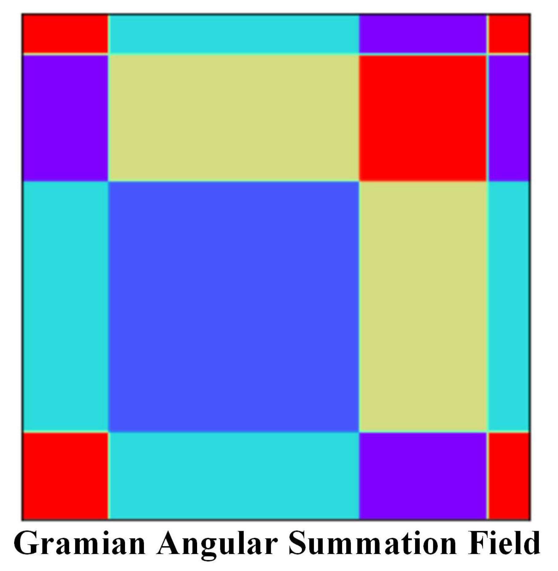
2.3. Gramian Angular Field (GAF)

GAF converts one-dimensional time series data into two-dimensional images and converts polar coordinate system data while preserving the correlation between each time point. This is suitable for analyzing data over brief lengths of time. The fundamental theory of Gramian angular field (GAF) can refer to the relative investigations [48,49,50]. If the time series data X = {x₁, x₂, x₃, …, x_n}, and then using the normalization method to scale all x values to the range of [−1, 1], the formula would be as follows [48]:

$${\tilde{\mathrm{x}}}_{\mathrm{i}}=\frac{{(\mathrm{x}}_{\mathrm{i}}-{\max \left(\mathrm{X}\right))+(\mathrm{x}}_{\mathrm{i}}-\min \left(\mathrm{X}\right))}{\max \left(\mathrm{X}\right)-\min \left(\mathrm{X}\right)}$$

(5)

By calculating the arccosine using the time point as the radius and scale value, the polar coordinate system is generated [48]:

$$\left\{\begin{array}{cc}{\mathrm{\theta }}_{\mathrm{i}}{=\cos }^{-1}{(\tilde{\mathrm{x}}}_{\mathrm{i}})\hfill & -1 \le {\tilde{\mathrm{x}}}_{\mathrm{i}} \le 1\hfill \\ {\mathrm{r}}_{\mathrm{i}}=\frac{\mathrm{i}}{\mathrm{n}}\hfill & \hspace{1em}\hspace{1em} \mathrm{i} \in \mathrm{n}\hfill \end{array}\right.$$

(6)

${\mathrm{\theta }}_{\mathrm{i}}$ is the opposite value of the cosine function. ${\mathrm{r}}_{\mathrm{i}}$ is the radius of ${\mathrm{x}}_{\mathrm{i}}$ on the polar coordinate system. The data of [−1, 1] corresponds to the cosine angle which varies between [0, π]. The time correlation can be observed from the angle. The Gramian angular summation field (GASF) and Gramian angular difference field (GADF) can be obtained by calculating the sum/difference of the trigonometric function. This paper uses GASF, which is defined as follows [48]:

$$\mathrm{GASF}=\left(\begin{array}{ccc}\begin{array}{c}\cos \left({\mathrm{\theta }}_1{+\mathrm{\theta }}_1\right)\\ \cos \left({\mathrm{\theta }}_2{+\mathrm{\theta }}_1\right)\end{array}& \cdots & \begin{array}{c}\cos \left({\mathrm{\theta }}_1{+\mathrm{\theta }}_{\mathrm{n}}\right)\\ \cos \left({\mathrm{\theta }}_2{+\mathrm{\theta }}_{\mathrm{n}}\right)\end{array}\\ ⋮& \ddots & ⋮\\ \cos \left({\mathrm{\theta }}_{\mathrm{n}}{+\mathrm{\theta }}_1\right)& \cdots & \cos \left({\mathrm{\theta }}_{\mathrm{n}}{+\mathrm{\theta }}_{\mathrm{n}}\right)\end{array}\right)$$

(7)

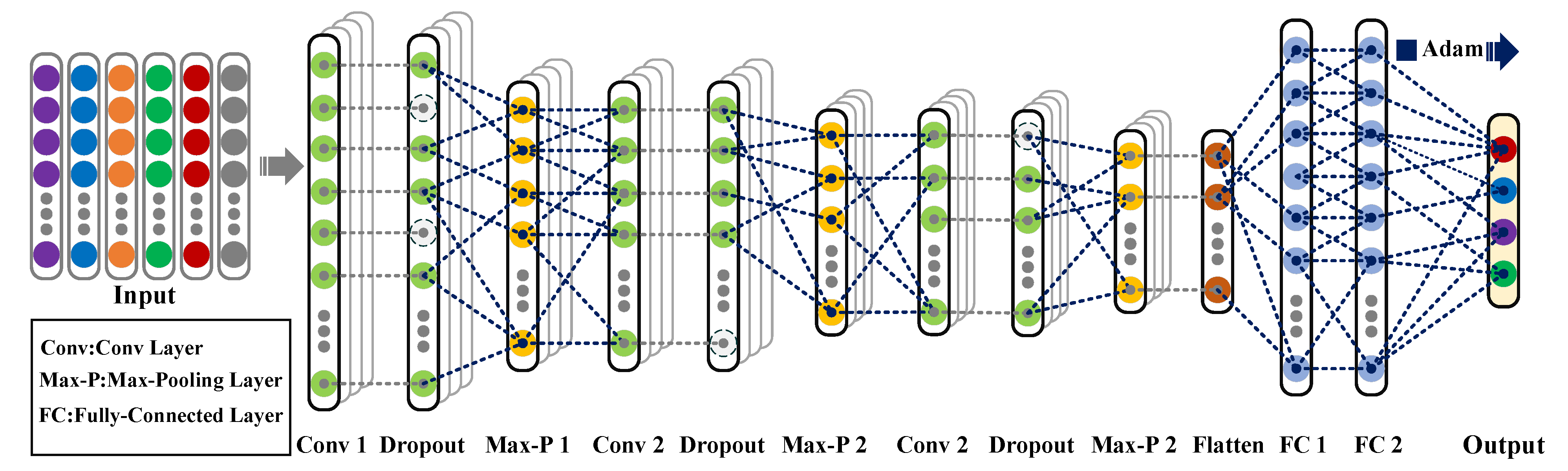
2.4. Convolutional Neural Network (CNN)

CNN is a deep feedforward neural network, which consists of convolutional layers, pooling layers, and fully connected layers. It processes 1D time series and 2D image data through convolution operations and can learn features from nonlinear and non-stationary signals. Image and pattern recognition works well. The fundamental theory of convolutional neural networks (CNN) can refer to the relative investigations [24,26,28,29,40].

2.4.1. Convolution Layer

The core of CNN is the convolutional layer. Adjusting the padding of the convolution kernel avoids image distortion and controls the stride size, reducing the number of input parameters and calculations. Different features are extracted through the sliding window of the convolution kernel to obtain a feature map, which can be expressed as the following equation [24]:

$${\mathrm{X}}_{\mathrm{j}}^{\mathrm{L}}=\mathrm{S}({\displaystyle \sum }_{\mathrm{i}ϵ{\mathrm{M}}_{\mathrm{j}}}{\mathrm{X}}_{\mathrm{i}}^{\mathrm{L}-1}·{\mathrm{w}}_{\mathrm{ij}}^{\mathrm{L}}{+\mathrm{b}}_{\mathrm{j}})$$

(8)

S is an activation function and uses the ReLU function as an activation function to enhance the nonlinear characteristics of the neural network and improve training speed. M_j is the input feature set. ${\mathrm{w}}_{\mathrm{ij}}^{\mathrm{L}}$ is the weight matrix. ${\mathrm{b}}_{\mathrm{j}}$ is the bias value of the convolutional layer.

2.4.2. Pooling Layer

The pooling layer processes the input features in the following sampling methods, including average pooling, maximum pooling, and random pooling. This paper utilizes the maximum pooling method to divide the input image into rectangular areas and output the maximum value for each sub-area, which can reduce the size of data space and the number of parameters. Overfitting can be improved and training time reduced. Max pooling is defined as [28]:

$${\mathrm{x}}_{\mathrm{i}}^{\mathrm{a},\mathrm{b}}{=\max (\mathrm{x}}_{\mathrm{i}}^{\acute{\mathrm{a}},\acute{\mathrm{b}}}: \mathrm{a} \le \acute{ \mathrm{a}} < \mathrm{a}+\mathrm{p}, \mathrm{b} \le \acute{ \mathrm{b}} < \mathrm{b}+\mathrm{p})$$

(9)

${\mathrm{x}}_{\mathrm{i}}^{\mathrm{a},\mathrm{b}}$ is the (a,b) pixel in the “i” feature map after processing. ${\mathrm{x}}_{\mathrm{i}}^{\acute{\mathrm{a}},\acute{\mathrm{b}}}$ is after processing. p is the pooling window step size.

2.4.3. Fully Connected Layer

After the final maximum pooling layer, all neurons are activated through the fully connected layer. The regression function of this layer uses the Softmax normalized exponential function to map the output value to the (0, 1) interval and obtains it in the form of a probability distribution classification result. Softmax can be expressed as follows:

$${\mathrm{\sigma }\left(\mathrm{z}\right)}_{\mathrm{i}}=\frac{{\mathrm{e}}^{\mathrm{zi}}}{{\sum }_{\mathrm{k}=1}^{\mathrm{K}}{\mathrm{e}}^{\mathrm{zk}}}\hspace{1em}\hspace{1em}\mathrm{for} \mathrm{i}=1,2,\dots ,\mathrm{K}$$

(10)

Softmax compresses the K-dimensional vector of any real number to a K-dimensional real vector $\mathrm{\sigma }\left(\mathrm{z}\right)$, so that each element is mapped between (0,1).

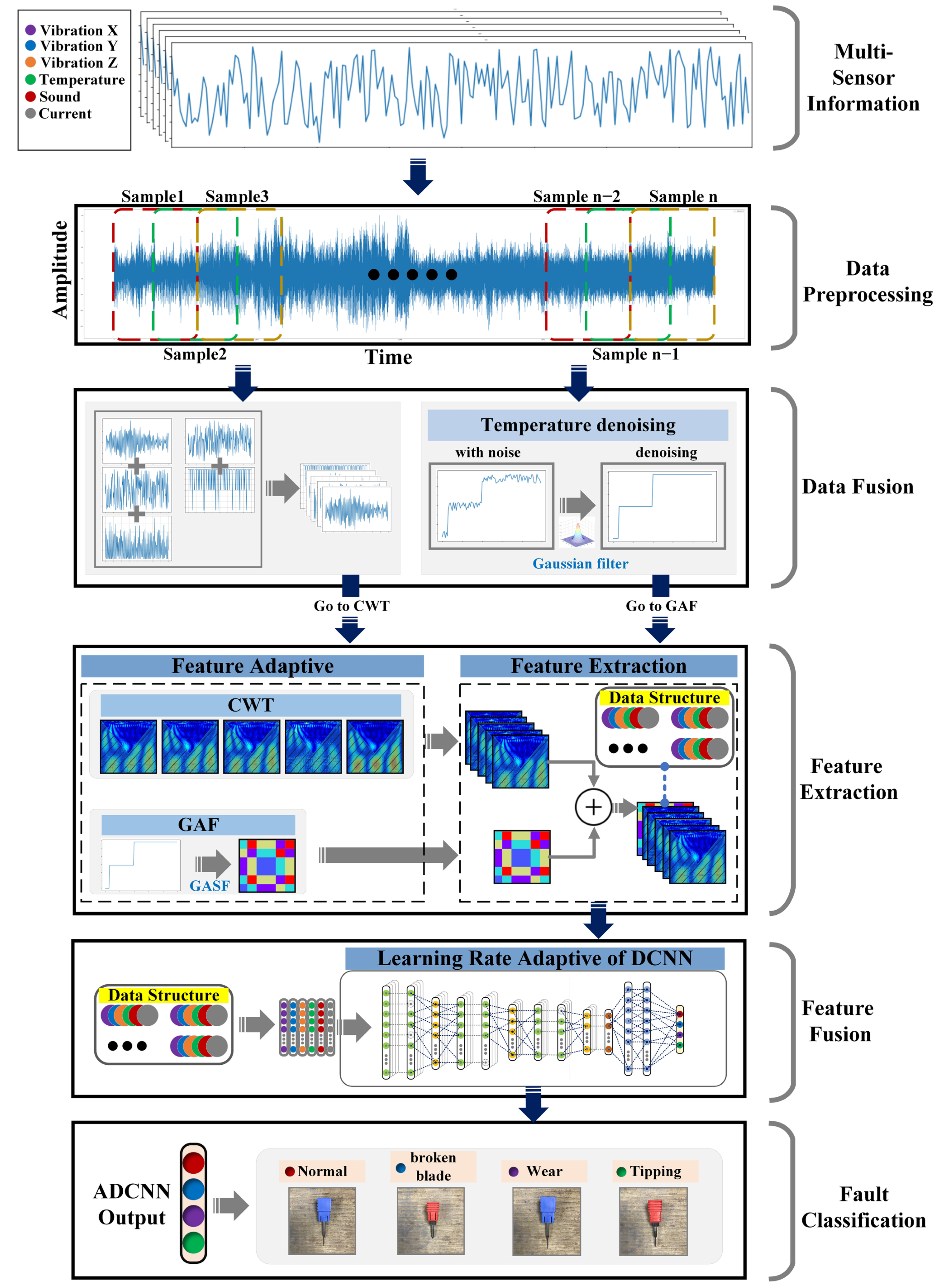
3. Adaptive Data Fusion Method Based on ADCNN for Fault Diagnosis

In this section, the fault diagnosis and classification method of ADCNN is introduced. The architecture is shown in Figure 1. There are six blocks in total. (1) Multi-sensor information: captures the raw data of mechanical equipment multi-sensors, including vibration X, vibration Y, vibration Z, temperature, sound, and six-dimensional data of electric currents. (2) Data preprocessing: uses a sliding window to divide data. (3) Data fusion: integrates the five-dimensional vibration X, vibration Y, vibration Z, sound, and non-stationary time-varying signals of the electric currents for array data structure fusion. Performs Gaussian filtering and de-noising processing for temperature-stationary signals. (4) Feature extraction: uses CWT to convert the data of vibration X, vibration Y, vibration Z, sound, and electric current channels to adaptive time–frequency map features of different frequency bands. Uses GAF to convert temperature data into GASF two-dimensional image features, and then fuses the six image channels to extract the features as the input of CNN. (5) Feature fusion: the convolutional layer processes the input features into feature maps, and the pooling layer performs adaptive feature fusion for downsampling. (6) Fault classification: uses the Softmax function to output the model prediction results.

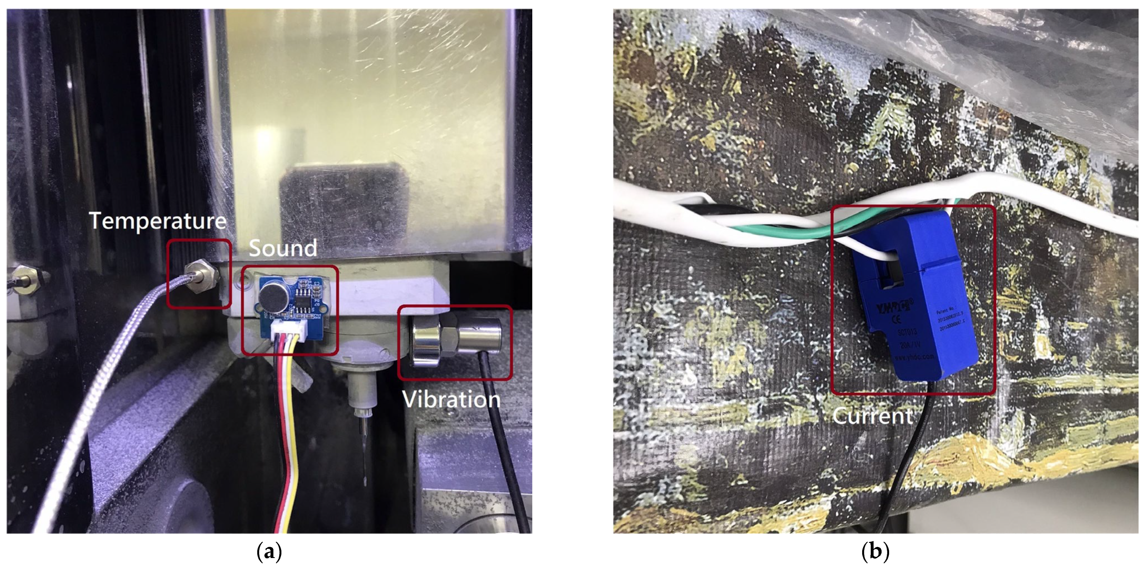
3.1. Multi-Sensor Information

Data-driven and feature fusion data sources. Jing et al. verified the effectiveness of multi-sensing data for fault prediction classification [42]. Real-time capturing of vibration X, vibration Y, vibration Z, temperature, sound, and electric current sensor-related data of rotating equipment with a plug-in device. Assuming that the sensing data sets ${\mathrm{X}}_1$ to ${\mathrm{X}}_{\mathrm{n}}$ are multi-sensor data vectors, the equation can be expressed as follows:

$${\mathrm{X}}_1=\left[{\mathrm{x}}_1{,\mathrm{x}}_2,\cdots {,\mathrm{x}}_{\mathrm{m}}\right]$$

(11)

$${\mathrm{X}}_{\mathrm{n}}=\left[{\mathrm{x}}_1{,\mathrm{x}}_2,\cdots {,\mathrm{x}}_{\mathrm{m}}\right]$$

(12)

In the experimental case of the dental processing machine, n is set to 6, representing 6 sensing data dimensions. Starting from 1 is vibration X, vibration Y, vibration Z, temperature, sound, and electric current sensing data.

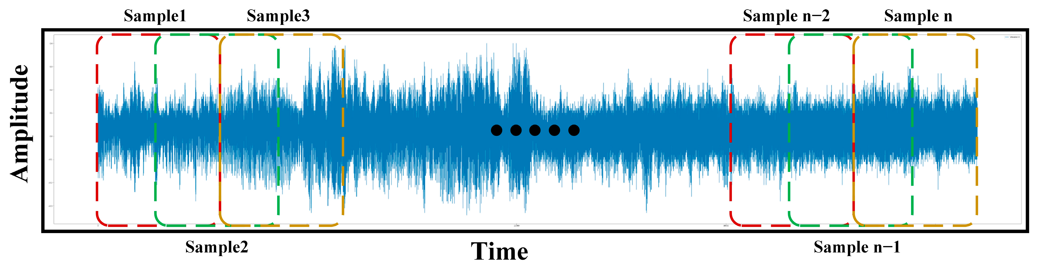
3.2. Data Preprocessing

Since the data range of each sensor is very different, when the multi-sensor data are fused it is easy to cause the gradient descent for finding the best solution. It takes many iterations to converge and improve the accuracy of the model. Therefore, data standardization must be normalized. The normalization method is min–max scaling, which is defined as:

$${\mathrm{x}}_{\mathrm{normalization}}=\frac{\mathrm{x}-\min \left(\mathrm{x}\right)}{\max \left(\mathrm{x}\right)-\min \left(\mathrm{x}\right)}$$

(13)

In order to improve the generalization ability of the model and avoid overfitting, ADCNN needs a large number of samples for training and testing. The sliding window sampling of the original time series data of each sensor achieves the effect of data enhancement [7]. Suppose that the time window length of the sample is n milliseconds, and the time step is 50% of the time window length, as shown in Figure 2.

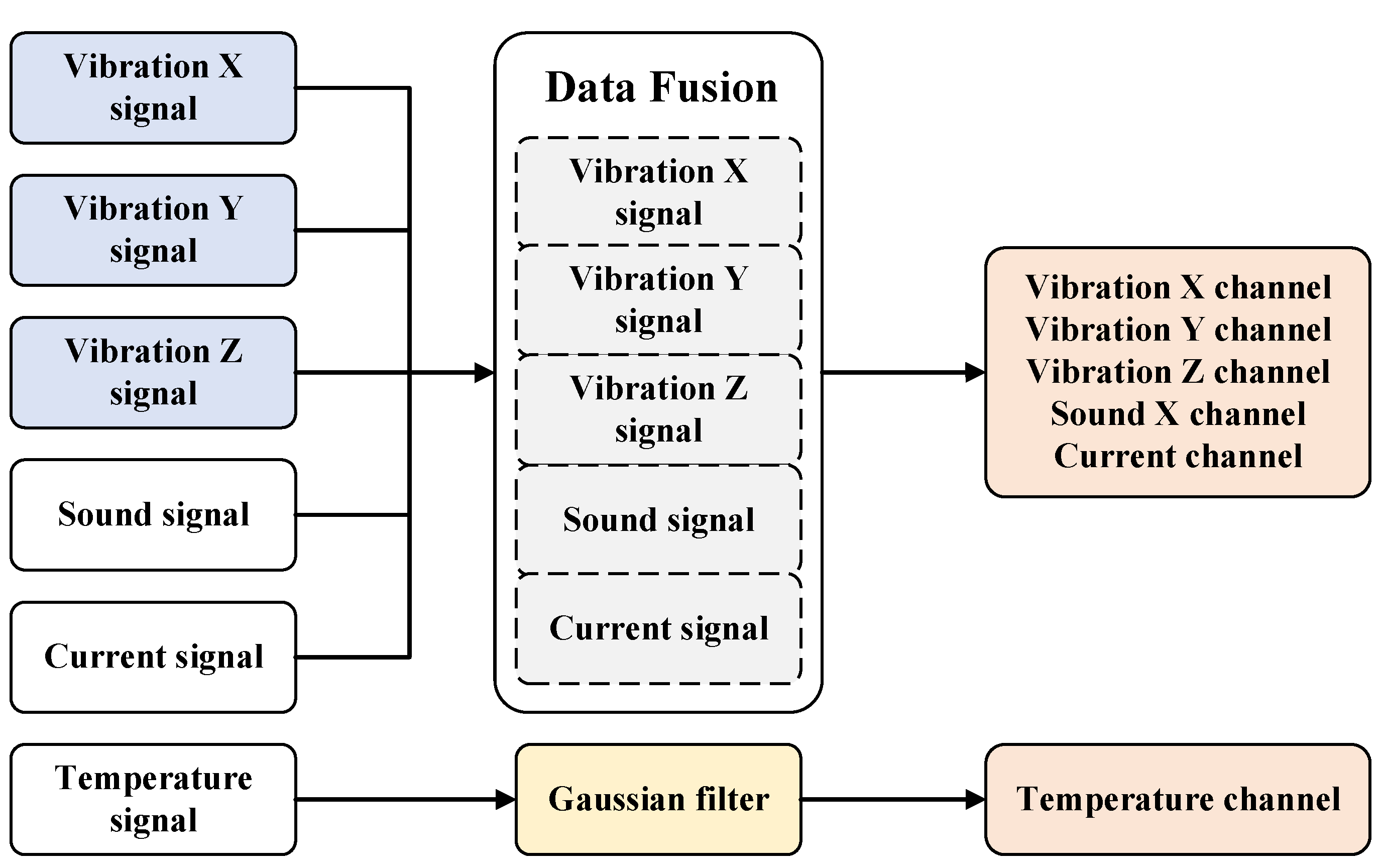
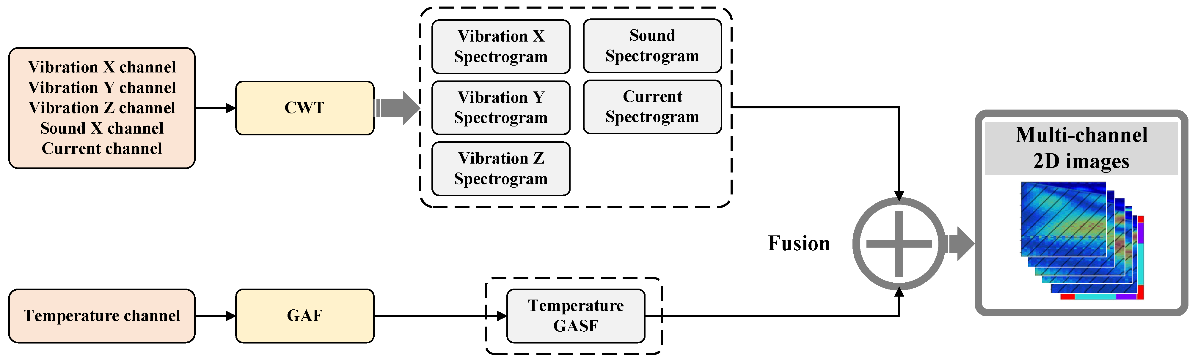
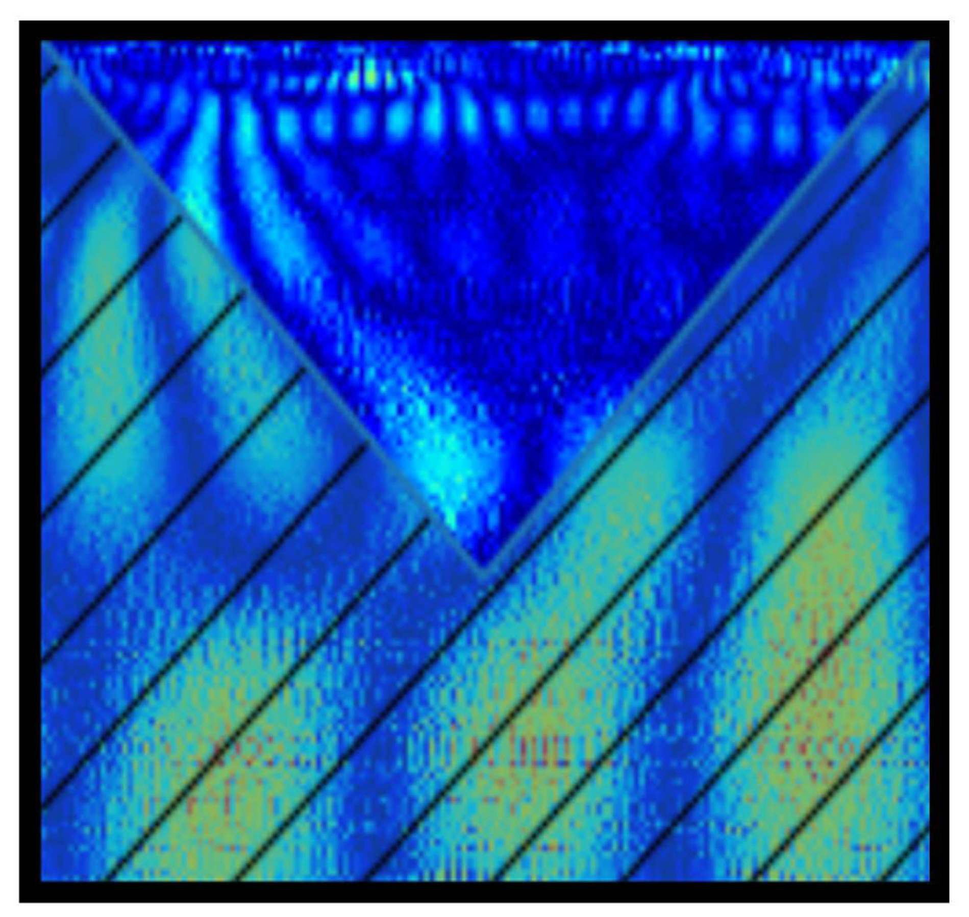
3.3. Data Fusion and Feature Extraction

Multi-sensing data fusion can preserve and complement the fault characteristics of different sensing signals at the same time, and its effectiveness has been verified in the literature and improved model prediction performance [14,15]. In order to preserve and strengthen the two-dimensional feature image input by CNN, the signals are divided into non-stationary, time-varying signals, and stationary signals. Vibration X, vibration Y, vibration Z, sound and electric current belong to the former, and data fusion of non-stationary time-varying signals is performed. The latter performs Gaussian filtering. The Gaussian filter has a good denoising and signal smoothing effect on time-stationary sequence signals, but it will ruin the signal structure weakening characteristics for non-stationary time-varying signals. The Gaussian filter of the experimental case is designed with a standard deviation of 3 and a filter size of 19. Assuming that the sensing data set X has n-dimensional sensing data and m samples, the non-stationary, time-varying signal data fusion matrix equation can be expressed as follows:

$$\mathrm{X}=\left[\begin{array}{cccc}{\mathrm{x}}_1^{\left(1\right)}& {\mathrm{x}}_2^{\left(1\right)}& \cdots & {\mathrm{x}}_{\mathrm{n}}^{\left(1\right)}\\ {\mathrm{x}}_1^{\left(2\right)}& {\mathrm{x}}_2^{\left(2\right)}& \cdots & {\mathrm{x}}_{\mathrm{n}}^{\left(2\right)}\\ ⋮& ⋮& \ddots & ⋮\\ {\mathrm{x}}_1^{\left(\mathrm{m}\right)}& {\mathrm{x}}_2^{\left(\mathrm{m}\right)}& \cdots & {\mathrm{x}}_{\mathrm{n}}^{\left(\mathrm{m}\right)}\end{array}\right]$$

(14)

Among them, the case n in this article is five channels, starting from one to correspond to vibration X, vibration Y, vibration Z, sound, and electric current sensing data. Figure 3 shows the process.

The feature extractor uses data multi-signal fusion matrix equation and the temperature vector data channels and converts them into multi-time–frequency images and two-dimensional images for feature extraction, fusing them into multi-channel image features. Figure 4 displays the flow chart.

Traditional signal analysis focuses on the time domain and frequency domain. Fourier transform has been applied to various analytical instruments; however, Fourier transform has the disadvantage of fixed time length and resolution and cannot effectively extract features for time-varying signals whose waveform cycles vary. The wavelet transform can dynamically and adaptively adjust the time resolution. When the high-frequency component has a short resolution, and the low-frequency component has a short resolution, the time–frequency domain features can be effectively extracted by adaptively adjusting the time length, increasing the robustness of the model prediction. The experimental case uses Morlet as the mother wavelet function. Morlet has been verified to effectively extract fault features from non-stationary signals and obtain good resolution in the time and frequency domains [28]. Morlet wavelet is defined as:

$${\mathrm{\phi }\left(\mathrm{x}\right)=\mathrm{e}}^{{-\mathrm{x}}^2}\cos (\mathrm{\pi }\sqrt{\frac{2}{\ln 2}\mathrm{x}})$$

(15)

Adjust the scale factor α of Formula (1) to obtain the scale factor of different signals in time. By stretching or shrinking the wavelet, slow or sudden changes in the signal can be recorded. In theory, the time step of the signal is multiplied by the scale factor to obtain the product. The wavelet coefficients of all the wavelet coefficients can be converted into images by converting the absolute values of all wavelet coefficients to obtain a scalogram in the time–frequency domain, as shown in Figure 5.

The Gaussian filter is used for denoising in order to prevent different noise interference in the production environment from affecting the GASF-converted image. Then GASF converts the temperature vector data into an image and calculates the polar coordinate system with Formula (6) to obtain the converted cosine angle of the temperature series data, switching between [0, π] in order to preserve the data correlation of time points. The case experiment uses Formula (7) to calculate the trigonometric function of GASF and then obtains a two-dimensional image of temperature time series for fault classification, as shown in Figure 6.

3.4. Feature Fusion

The core architecture of feature fusion is a deep convolutional neural network (DCNN), performing a feature-level fusion of input multi-channel image features, further optimizing the data structure, and then using adaptive learning rate Adam to perform gradient descent optimization training. Lastly, the normalized Softmax function is used for fault diagnosis and classification.

The DCNN architecture diagram is shown in Figure 7. The feature fusion includes three layers of convolution layers and pooling layers. The convolution layer uses convolution kernels to extract high-level features of multi-source input. ReLu enhances the nonlinear capability of the model. The pooling layer uses 2 × 2 maximum pooling to extract the important features of the feature map to enhance the model’s anti-noise ability, and at the same time compresses the feature dimension to reduce the computational complexity, so that the training speed can be accelerated and converged. In order to avoid overfitting, the model adds a Dropout between the convolutional layer and the pooling layer and randomly discards 30% of the neurons during each training. The gradient of the discarded neurons is 0, so each training reduces dependencies between random neurons. After the three-level convolution and pooling layers for feature fusion, the fused feature map is flattened into one-dimensional vector data and input to the fully connected layer classifier for fault prediction and classification. For the loss function, categorical cross-entropy is selected with the activation function Softmax to re-adjust the model output, which has a good effect on multi-classification problems. Categorical cross-entropy can effectively measure the distinguishability between discrete probability distributions. The loss of the sample can be calculated by the following formula:

$$\mathrm{Loss}=-{\displaystyle \sum }_{\mathrm{i}=1}^{\begin{array}{c}\mathrm{output}\\ \mathrm{size}\end{array}}{\mathrm{y}}_{\mathrm{i}}·{\log \hat{\mathrm{y}}}_{\mathrm{i}}$$

(16)

Output size is the number of scalar values in the model output. ${\mathrm{y}}_{\mathrm{i}}$ is the corresponding target value, ${\hat{\mathrm{y}}}_{\mathrm{i}}$ is the i-th scalar value.

The Softmax function maps the probability distribution of each classification result and compresses the K-dimensional vector containing any real number into another K-dimensional vector, so that the range of the classification results is between (0, 1), and the sample vector X belongs to the “j”. The probability of classification is:

$$\mathrm{P}(\mathrm{y}=\mathrm{j}|\mathrm{X})=\frac{{\mathrm{e}}^{{\mathrm{X}}^{\mathrm{T}}{\mathrm{W}}_{\mathrm{j}}}}{{\sum }_{\mathrm{k}=1}^{\mathrm{K}}{\mathrm{e}}^{{\mathrm{X}}^{\mathrm{T}}{\mathrm{W}}_{\mathrm{k}}}}$$

(17)

The stochastic gradient descent optimization method of the model is adaptive moment estimation (Adam). Traditionally, the network weights use a fixed learning rate to update the weights and biases during training, which is prone to low computational efficiency and the inability to effectively find the global minimum. For the global minimum value issue, Adam combines the advantages of the adaptive gradient algorithm (AdaGrad) and root mean square propagation (RMSProp) to dynamically adjust the learning rate according to the gradient to improve sparse gradients and uses an exponential moving average to maintain the average value of the weight gradient magnitudes, which can adaptively reduce the effect of noise in non-stationary signal classification models. Adam’s formula for updating weights and biases is:

$$\left\{\begin{array}{c}{\mathrm{w}}^{\prime }=\mathrm{w}-\mathrm{\eta }\frac{\partial \mathrm{J}(\mathrm{w},\mathrm{b})}{\partial \mathrm{w}}\\ {\mathrm{b}}^{\prime }=\mathrm{b}-\mathrm{\eta }\frac{\partial \mathrm{J}(\mathrm{w},\mathrm{b})}{\partial \mathrm{b}}\end{array}\right.$$

(18)

3.5. Fault Classification

The fault classification displays the results of the prediction and diagnosis of rotating machinery. The experimental case in this paper predicts the fault classification of the dental cutter. ADCNN outputs the malfunction probability distribution of the four classifications through Softmax. There are four classification results: (1) normal, (2) breaking, (3) wear, and (4) tipping.

4. Experiment and Discussion

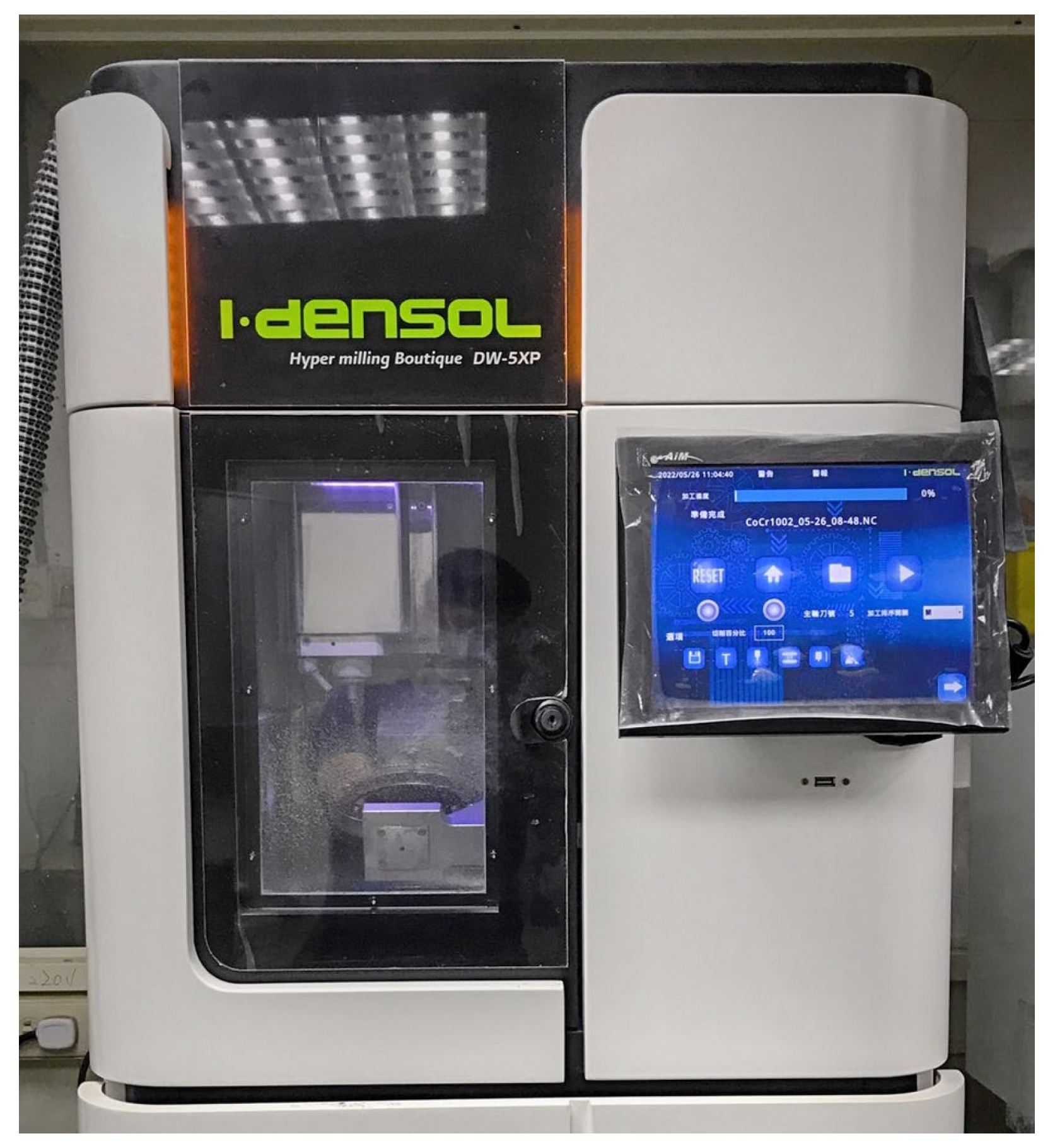
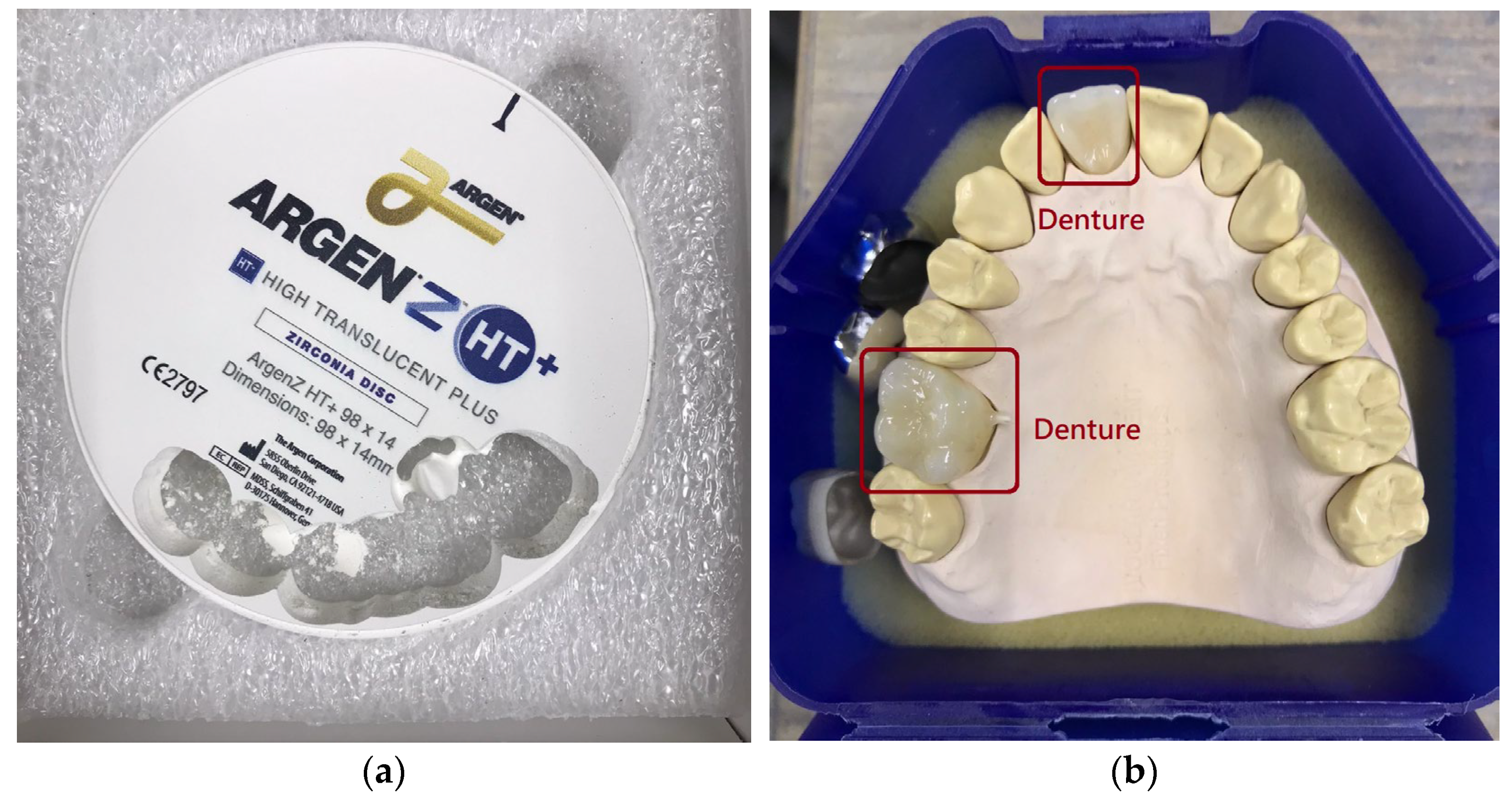
4.1. Experiment Setup

This experiment’s data were collected at the Certified Dental Institute. The dental milling machine’s serial number was: DW-5XP. To evaluate the effectiveness of the proposed method, a 2 mm diameter tungsten steel drill was used to process zirconia dentures. Figure 8 shows the experimental platform, and Figure 9 shows the materials and dental mold products. The experimental environment utilizes the Tensorflow architecture and keras API; the development language uses Python and related packages for development; the testing hardware is a notebook computer whose configuration is i7-11800H, 64 G RAM, and RTX3070 with built-in GPU computing.

The sensor installation is shown in Figure 10. A total of three-axis vibration accelerometers, namely temperature, sound, and current sensors are set up. At the same time, different physical characteristics data of tool faults are captured. The sampling frequency is 10 KHz, and the sampling time of the data set is 5 s, for a total of 200,000 points of data.

During the experiment, dental mold cutting tests were performed with various cutters, including normal, breaking, worn, and tipping. The cutters are shown in Figure 11. Machine speed was 20,000 rpm, and the data were collected by cutting the same dental mold from the same patient. The processing status and dataset labels are shown in

Table 1. Processing status and labeling table.

Type Label	Health Condition	Description	Processing Speed (rpm)
0	Normal	Normal processing	20,000
1	Breaking	Overheated or too dull and resulted in breaking	20,000
2	Wear	Poor quality of dentures due to wear that is visually undetectable	20,000
3	Tipping	Overheating or too dull and resulted in tipping	20,000

.

4.2. Dataset

The experiment data dimensions are 7-dimensional columns: the 6-dimensional input and the 1-dimensional output. The four fault classifications have a total of 200,000 sampling points, and the input sample length is 20 milliseconds. In order to ensure that the sampling points of the signal feature samples can be completely preserved, it is set to 200 points. After data enhancement, there are 1988 data samples, and the fault classification samples are all the same at 497. During model training, 80% of the data samples are randomly selected as the training set, 80% are the test set, and 20% of the data samples in the training set are used as the validation set for model training and verification. Lastly, fault classification model tests are performed.

4.3. Parameter Selection for the DCNN Model

The DCNN model architecture and parameters used in this paper are shown in

Table 2. DCNN table of model structures.

Layer	Parameter Name	Parameter Size	Output Size
Input	/	/	127 × 127 × 3
Conv1	Convolutional kernel	5 × 5	123 × 123 × 32
Dropout	Dropout neuron ratio	30%	/
Max-p1	Max pooling kernel	2 × 2	61 × 61 × 32
Conv2	Convolutional kernel	5 × 5	57 × 57 × 64
Dropout	Dropout neuron ratio	30%	/
Max-p2	Max pooling kernel	2 × 2	28 × 28 × 64
Conv3	Convolutional kernel	5 × 5	24 × 24 × 64
Dropout	Dropout neuron ratio	20%	/
Max-p3	Max pooling kernel	2 × 2	12 × 12 × 64
FC1	Fully connected neuron	1000	9216 × 1000 + 1000
FC2	Fully connected neuron	4	1000 × 4 + 4
Output	Weight matrix	4004 × 4	4 × 1

. The convolutional kernel of the first three convolutional layers is designed with a large convolutional kernel size of 5 × 5 to extract the main features of the image. Dropout randomly discards 30%, 30%, and 20% of neurons in sequence to reduce over-fitting during training, and the subsequent max pooling layer is designed in the following sampling method. The size of the max pooling kernel is 2 × 2, integrating subtle and important features to enhance the model’s anti-noise ability while reducing the computational complexity and improving the training convergence rate. The latter two-layer fully connected neurons are designed to be 1000 or 4, which improves the training effect, output prediction, and classification results.

4.4. Experimental Results

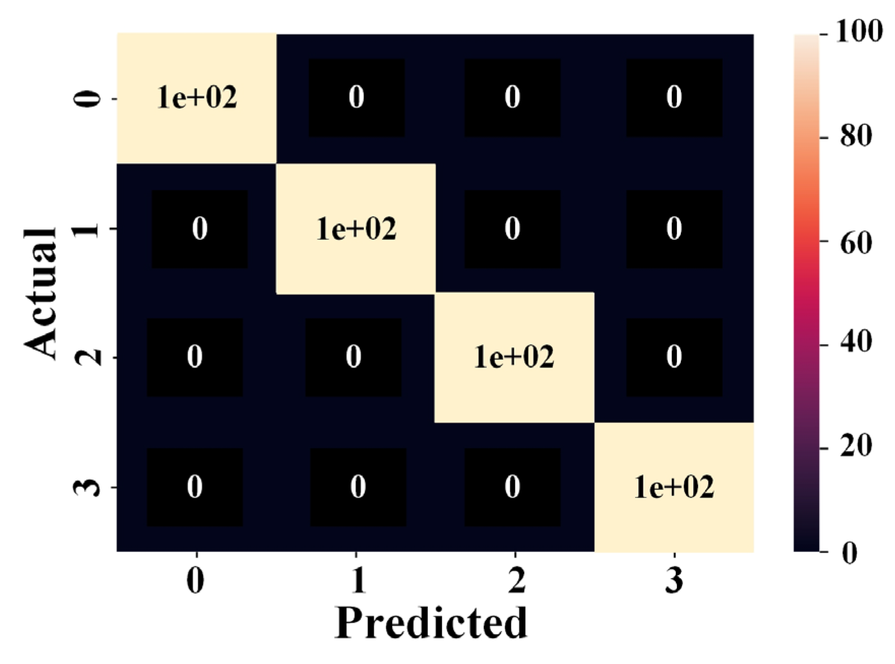
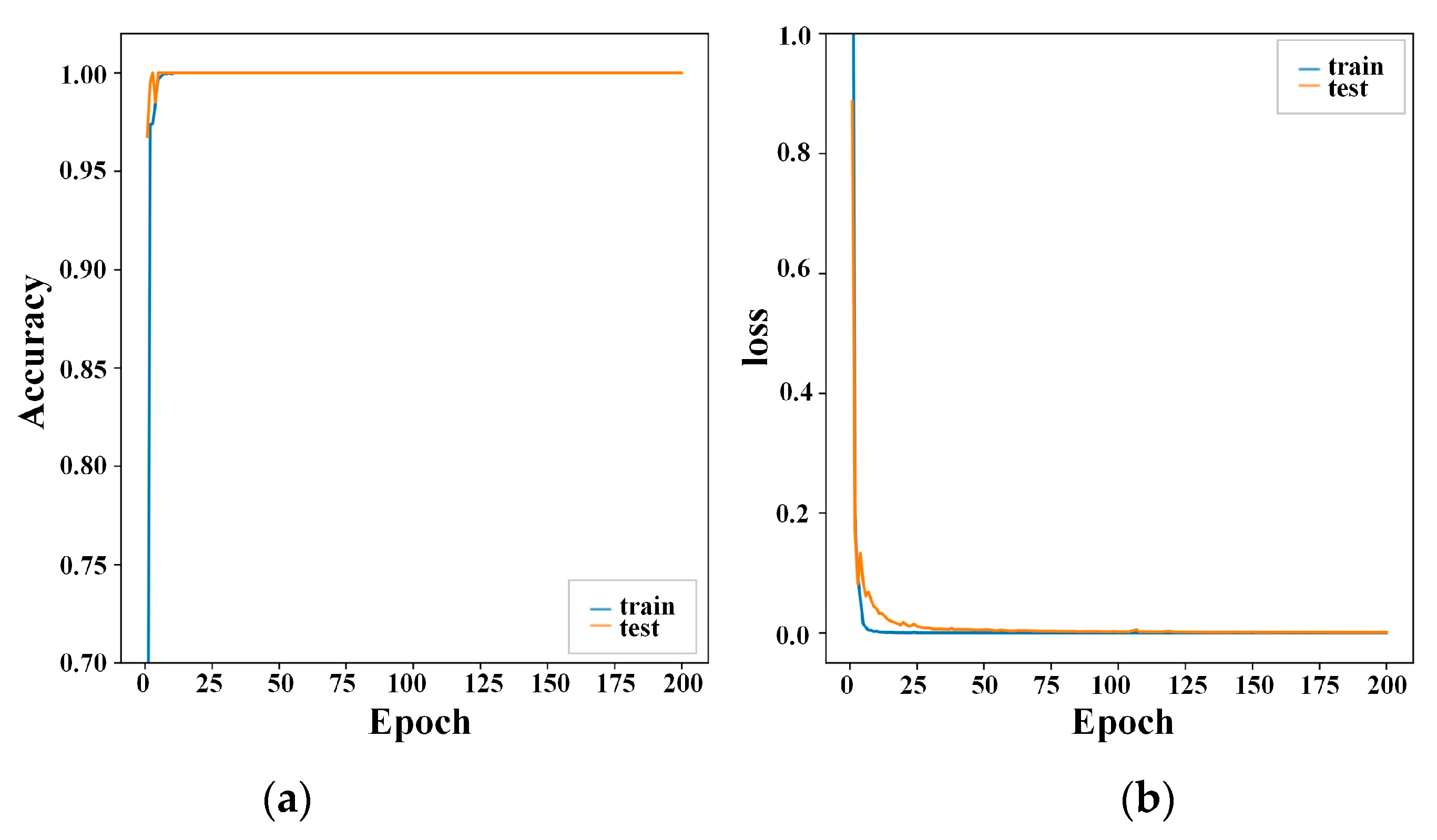
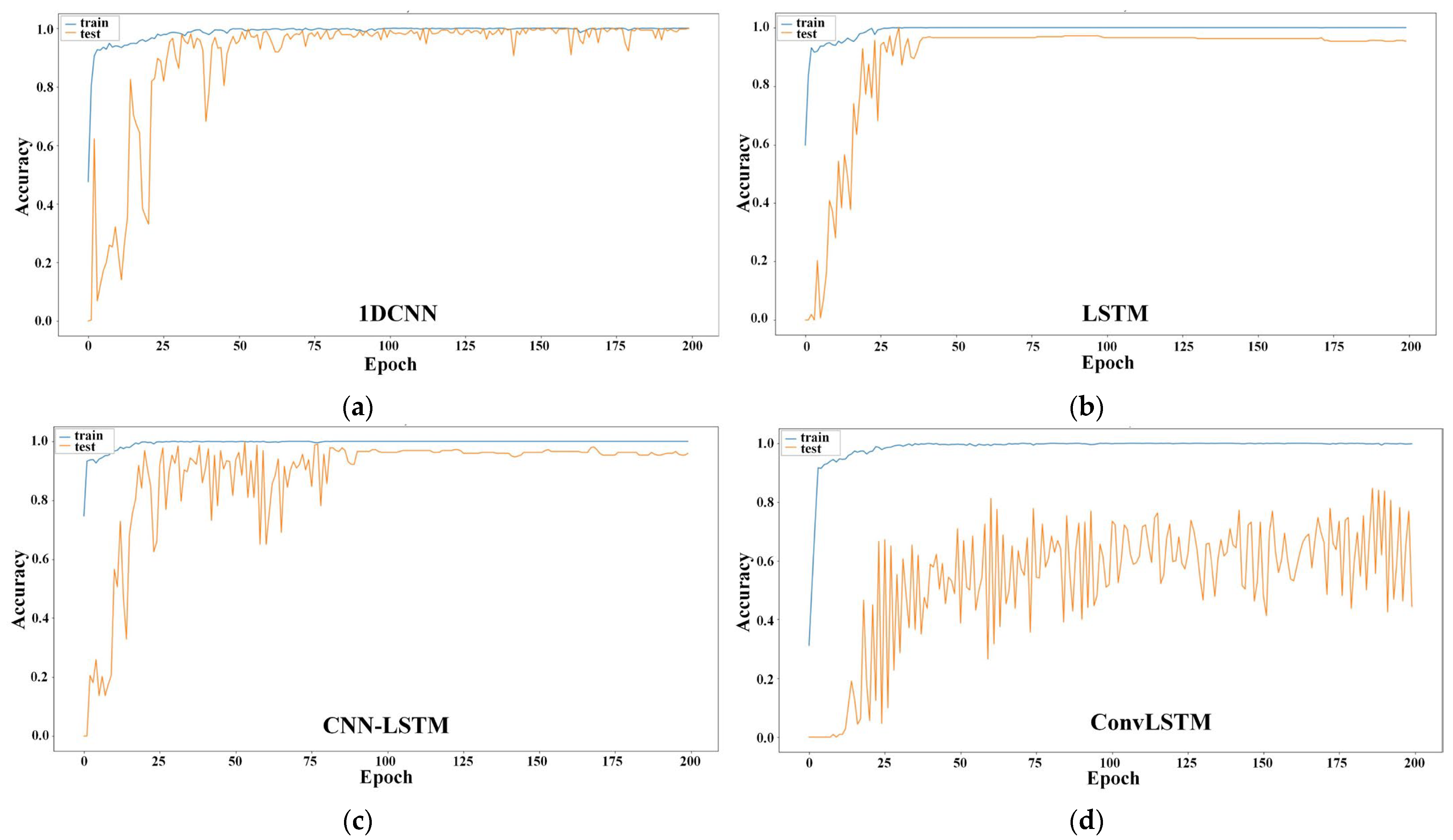
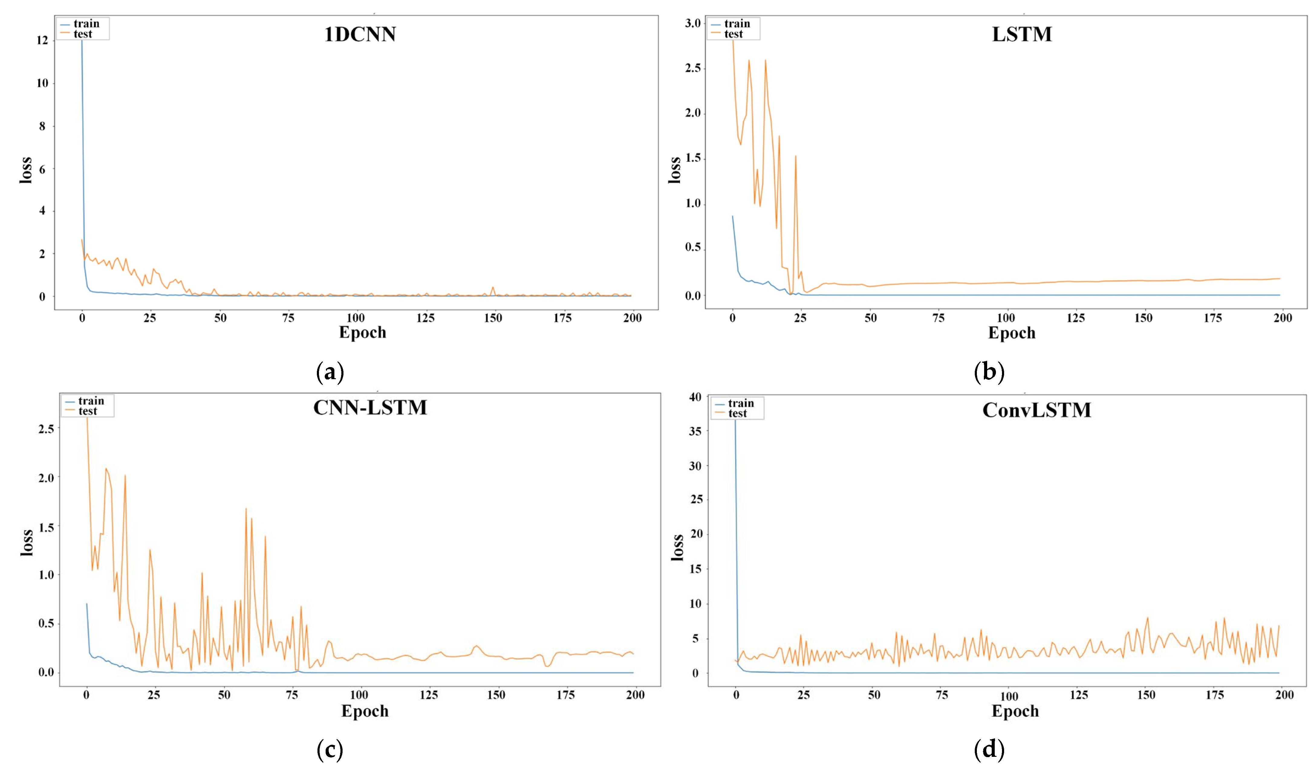
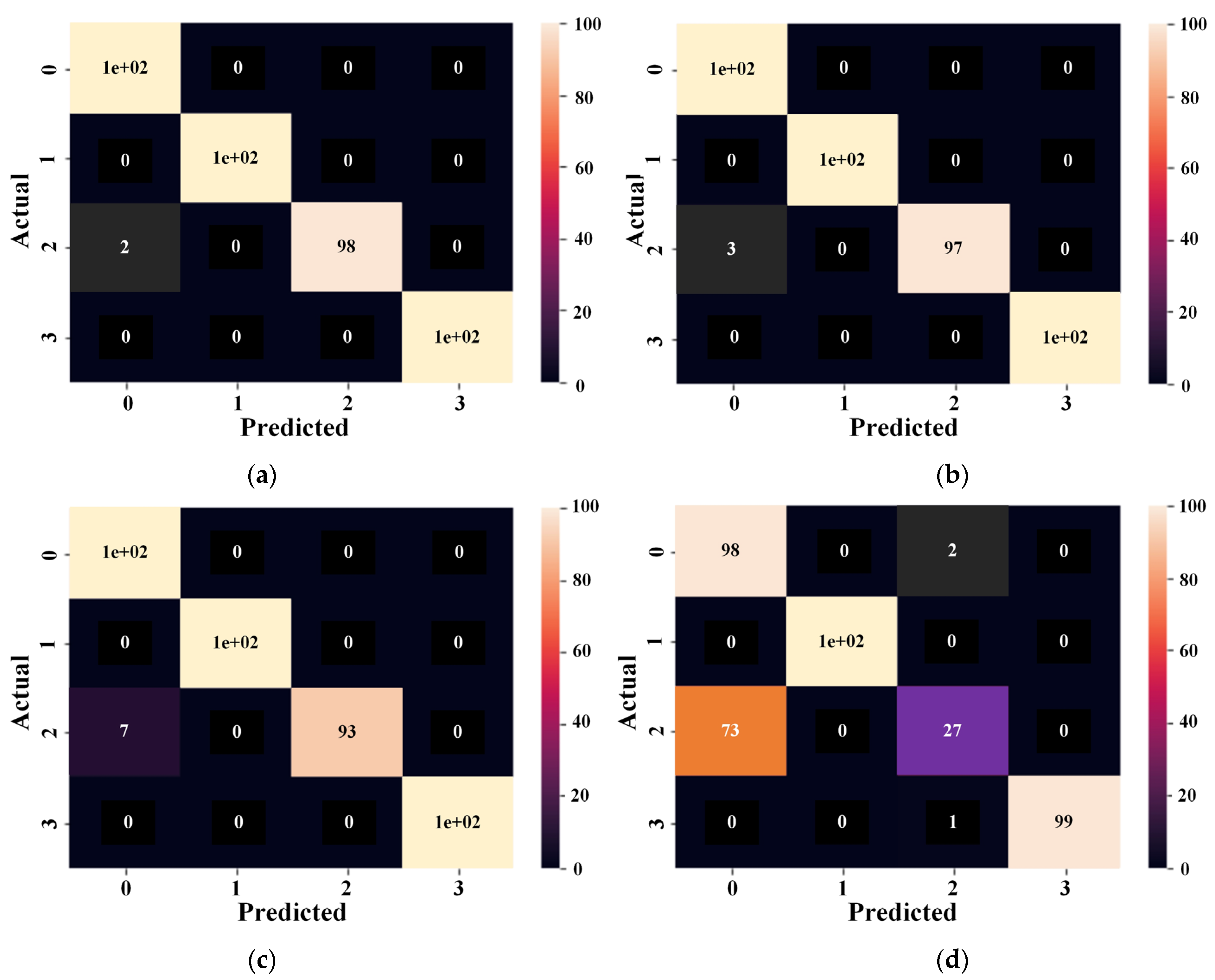
4.4.1. Performance Validation of the ADCNN Model

The fault diagnosis experiment was carried out on the dental milling machine using ADCNN, and the weights and deviations were optimized by the training of the model. Figure 12 shows the accuracy and loss of the experiment results. Figure 12a shows that the model training’s accuracy is close to 100%, and the epoch quickly converges after 40 training cycles. The loss curve indicates a rapid decline and steady convergence after 45 training epochs. Simultaneous observation of Figure 12a,b show that the model has almost no overfitting, indicating that the learning and prediction of the model are robust.

To verify the superiority of the proposed method, it was compared with four popular models, namely 1DCNN, LSTM, CNN-LSTM, and ConvLSTM. The same six data sets were tested with 1600 training samples and 400 test samples. The parameters were set with the same epoch and batch size. A dropout layer was also added to reduce overfitting. For this experiment, the epoch was set to 200 times, and the batch size was set to 128. The results of the accuracy of the four models are shown in Figure 13. The 1D-CNN’s verification accuracy (the orange line) was the highest, but it may not converge. Although the results of LSTM and CNN-LSTM show convergence, there was also some overfitting. ConvLSTM results were the worst; not only was the accuracy of the verification fairly low, but it also had issues with vibration and the inability to converge.

Figure 14 shows the experimental results of the loss of the four models. The results show that the verification loss (orange line) of 1DCNN is the lowest and close to 0, but there was some vibration. Overfitting occurs for both LSTM and CNN-LSTM, and the ConvLSTM results were the worst, with obvious vibrations and an inability to converge.

In order to observe the performance of all comparison methods in classifying dental milling machine tool failures, the confusion matrix is used. As shown in Figure 15, the ADCNN did not classify incorrectly during testing. Figure 16a is the confusion matrix of 1DCNN, which shows that there were two prediction errors that the tool was normal, but it was actually worn. Figure 16b is the confusion matrix of LSTM, which shows that there were three errors in predicting that the tool was normal but was actually worn. Figure 16c is the confusion matrix of CNN-LSTM, showing seven errors in predicting that the tool is normal but was actually worn. Figure 16d is the confusion matrix of ConvLSTM, showing 73 errors in predicting that the tool is normal but was actually worn, as well as three other errors. The confusion matrix results show that the most errors were when they were actually worn yet predicted as normal tools. It shows that the differences between the characteristics of the normal processing tools and the worn tools are minuscule, making it difficult to correctly predict the classification. All other classification items have significant features and classifications can be accurately predicted. The results show that the proposed ADCNN method can strengthen the classification of subtle features and also has excellent prediction performance.

The experiment of predicting classification accuracy uses the test set for model prediction. All methods are averaged after ten tests to draw a bar graph. The results are shown in Figure 17. The figure shows that ADCNN has the highest prediction accuracy at 100%, and ConvLSTM has the worst accuracy at 77.32%.

4.4.2. Performance Validation with Noise

In order to verify that the proposed method has adaptive anti-noise abilities in harsh production environments, white noise is added to the experiment to simulate the influence of noise on the prediction ability of the model. White noise is uniformly distributed noise and is defined as:

$$\mathrm{p}\left(\mathrm{z}\right)=\left\{\begin{array}{ll}1/2& \mathrm{if} -1\le \mathrm{z}\le 1\\ 0& \mathrm{otherwise}\end{array}\right.$$

(19)

z is between −1 and 1.

The signal-to-noise ratio (SNR) of the original signal and the noise is calculated by the following equation:

$${\mathrm{SNR}=10\log }_{10}{\left[\frac{{\mathrm{A}}_{\mathrm{signal}}}{{\mathrm{A}}_{\mathrm{noise}}}\right]}^2\left(\mathrm{dB}\right)$$

(20)

A_signal is the signal amplitude, A_noise is the noise amplitude, and the experiment design is 5 to 1, so the SNR is about 7 dB, indicating that the added white noise is a strong interference signal. Taking the X-axis vibration signal as an example, adding white noise results in Figure 18, showing that the original signal has been disturbed by noise, which slightly damages the original signal waveform.

The confusion matrices of the results of adding white noise are shown in Figure 19 and Figure 20, and the bar graph in Figure 21 shows the test accuracy of all comparison methods with added white noise. After ten experiments, the average of each method is calculated to create the bar graph. Figure 19 and Figure 21 show that ADCNN had four errors when predicting a normal machining tool. This indicates that there is a certain degree of adaptive anti-noise ability towards white noise, which can suppress the interference of the noise and reduce the decline of the model prediction accuracy. Figure 20 and Figure 21 show that the prediction accuracy of other comparative methods after adding noise had a larger decline than the method proposed in this paper, while CNN-LSTM had a smaller decline but lower accuracy. The results show that the proposed method is robust in a high-noise environment.

4.5. Discussion

This experimental design is a comparison between our proposed ADCNN method and four currently popular methods. The differences between an excessively worn dental milling cutter and a normal cutter are not very noticeable. Because of this, classification errors often occur; the prediction is that the cutter is normal when in fact it is worn. Our results show that ADCNN can accurately predict the difference between the normal cutter and the excessively worn cutter, whereas the other methods predict incorrectly. The addition of white noise reduced the accuracy of the proposed method from 100% to 99%, 1DCNN from 99.33% to 96.2%, LSTM from 99.05% to 94.1%, CNN-LSTM from 97.85% to 96.2%, and ConvLSTM from 77.32% down to 72.75%. The results show that, with or without noise interference, the proposed method has the highest prediction accuracy and adaptive anti-noise ability compared with the other methods.

Experiments show that fusion architecture and multi-sensing data’s feature extraction mechanism not only obtains subtler features but model classification accuracy is also improved through different physical signal characteristics. A white noise simulation model with an SNR of 7 dB is added to the adaptive ability of noise in the interference field of this experiment. The final classification accuracy is higher than other models, and it can also effectively classify normal tools and worn tools with minuscule characteristic differences. The traditional method requiring experts to de-noise the signal first and then extract features can also be bypassed, as some useful features may be lost during the de-noising process.

Furthermore, for model prediction robustness, Figure 12, Figure 13 and Figure 14 show that overfitting can be avoided with the proposed method. In comparison with other methods, the feature learning ability also has significant improvement. Feature fusion methods can improve the robustness and reliability of fault diagnosis.

5. Conclusions

This paper proposes a fault diagnosis method for rotating machinery based on adaptive multi-level input features, which can enhance the robustness of model prediction in complex noise environments. A dental milling machine is used to carry out the experiment of predicting tool classifications. The results show that, without the addition of white noise, the proposed ADCNN model can accurately predict the classification of four tools in the experiment. In comparison with the other four methods, ADCNN has the highest classification accuracy. The prediction error mostly misjudged tools as normal when they were in fact worn; this shows us that the feature differences between the normal and wear of the tools of the dental milling machine are subtle. This is also one of the key issues currently encountered in the dental milling process. The proposed method can accurately classify the normal and wear of the tool. In order to verify the robustness of the model, white noise was added to conduct experiments. The classification accuracy of the proposed method is as high as 99%, and it has a higher anti-noise ability than other control methods. It is able to realize adaptive multi-level fusion enhancement features and achieve robustness, making up for the shortcomings of traditional predictive fault classification and diagnosis methods.

References

1. Vununu, C.; Kwon, K.R.; Lee, E.J.; Moon, K.S.; Lee, S.H. Automatic Fault Diagnosis of Drills Using Artificial Neural Networks. In Proceedings of the 2017 16th IEEE International Conference on Machine Learning and Applications (ICMLA), Cancun, Mexico, 18–21 December 2017; pp. 992–995. [Google Scholar]
2. Senjoba, L.; Sasaki, J.; Kosugi, Y.; Toriya, H.; Hisada, M.; Kawamura, Y. One-Dimensional Convolutional Neural Network for Drill Bit Failure Detection in Rotary Percussion Drilling. Mining 2021, 1, 297–314. [Google Scholar] [CrossRef]
3. Wu, L.; Dong, Z.; Li, W.; Jing, C.; Qu, B. Well-Logging Prediction Based on Hybrid Neural Network Model. Energies 2021, 14, 8583. [Google Scholar] [CrossRef]
4. Wieczorek, G.; Chlebus, M.; Gajda, J.; Chyrowicz, K.; Kontna, K.; Korycki, M.; Jegorowa, A.; Kruk, M. Multiclass Image Classification Using GANs and CNN Based on Holes Drilled in Laminated Chipboard. Sensors 2021, 21, 8077. [Google Scholar] [CrossRef]
5. Mahmood, J.; Mustafa, G.-E.; Ali, M. Accurate estimation of tool wear levels during milling, drilling and turning operations by designing novel hyperparameter tuned models based on LightGBM and stacking. Measurement 2022, 190, 110722. [Google Scholar] [CrossRef]
6. Pradeep Kumar, D.; Muralidharan, V.; Ravikumar, S. Histogram as features for fault detection of multi point cutting tool—A data driven approach. Appl. Acoust. 2022, 186, 108456. [Google Scholar] [CrossRef]
7. Si, Y.; Li, X.; Kong, L.; Zhen, J.; Li, Y. Improved empirical wavelet denoising algorithm with application to whirling detection in deep hole drilling process. Procedia CIRP 2021, 104, 1924–1929. [Google Scholar] [CrossRef]
8. Pham, M.-T.; Kim, J.-M.; Kim, C.-H. 2D CNN-Based Multi-Output Diagnosis for Compound Bearing Faults under Variable Rotational Speeds. Machines 2021, 9, 199. [Google Scholar] [CrossRef]
9. van den Hoogen, J.; Bloemheuvel, S.; Atzmueller, M. Classifying Multivariate Signals in Rolling Bearing Fault Detection Using Adaptive Wide-Kernel CNNs. Appl. Sci. 2021, 11, 11429. [Google Scholar] [CrossRef]
10. Ji, M.; Peng, G.; He, J.; Liu, S.; Chen, Z.; Li, S. A Two-Stage, Intelligent Bearing-Fault-Diagnosis Method Using Order-Tracking and a One-Dimensional Convolutional Neural Network with Variable Speeds. Sensors 2021, 21, 675. [Google Scholar] [CrossRef]
11. Zhai, S.; Wang, Z.; Gao, D. Bearing Fault Diagnosis Based on a Novel Adaptive ADSD-gcForest Model. Processes 2022, 10, 209. [Google Scholar] [CrossRef]
12. Yang, Z.; Yang, R.; Huang, M. Rolling Bearing Incipient Fault Diagnosis Method Based on Improved Transfer Learning with Hybrid Feature Extraction. Sensors 2021, 21, 7894. [Google Scholar] [CrossRef] [PubMed]
13. Li, S.; Liu, G.; Tang, X.; Lu, J.; Hu, J. An Ensemble Deep Convolutional Neural Network Model with Improved D-S Evidence Fusion for Bearing Fault Diagnosis. Sensors 2017, 17, 1729. [Google Scholar] [CrossRef] [Green Version]
14. Jiang, Y.; Xia, T.; Wang, D.; Zhang, K.; Xi, L. Joint adaptive transfer learning network for cross-domain fault diagnosis based on multi-layer feature fusion. Neurocomputing 2022, 487, 228–242. [Google Scholar] [CrossRef]
15. Zhang, Y.; He, L.; Cheng, G. MLPC-CNN: A multi-sensor vibration signal fault diagnosis method under less computing resources. Measurement 2022, 188, 110407. [Google Scholar] [CrossRef]
16. Pacella, M.; Papadia, G. Fault Diagnosis by Multisensor Data: A Data-Driven Approach Based on Spectral Clustering and Pairwise Constraints. Sensors 2020, 20, 7065. [Google Scholar] [CrossRef] [PubMed]
17. Zhang, N. Research on Automatic Fault Diagnosis System of Coal Mine Drilling Rigs based on Drilling Parameters. In Proceedings of the 2019 IEEE 4th Advanced Information Technology, Electronic and Automation Control Conference (IAEAC), Chengdu, China, 20–22 December 2019; pp. 2373–2377. [Google Scholar]
18. Oh, D.C.; Jo, Y.U. EMG-based hand gesture classification by scale average wavelet transform and CNN. In Proceedings of the 2019 19th International Conference on Control, Automation and Systems (ICCAS), Jeju, Republic of Korea, 15–18 October 2019; pp. 533–538. [Google Scholar]
19. Xie, Y.; Zhang, T. Feature extraction based on DWT and CNN for rotating machinery fault diagnosis. In Proceedings of the 2017 29th Chinese Control and Decision Conference (CCDC), Chongqing, China, 28–30 May 2017; pp. 3861–3866. [Google Scholar]
20. Eltotongy, A.; Awad, M.I.; Maged, S.A.; Onsy, A. Fault Detection and Classification of Machinery Bearing Under Variable Operating Conditions Based on Wavelet Transform and CNN. In Proceedings of the 2021 International Mobile, Intelligent, and Ubiquitous Computing Conference (MIUCC), Cairo, Egypt, 26–27 May 2021; pp. 117–123. [Google Scholar]
21. Huang, D.; Zhang, W.A.; Guo, F.; Liu, W.; Shi, X. Wavelet Packet Decomposition-Based Multiscale CNN for Fault Diagnosis of Wind Turbine Gearbox. IEEE Trans. Cybern. 2021, 53, 443–453. [Google Scholar] [CrossRef]
22. Wang, T.; Lu, C.; Sun, Y.; Yang, M.; Liu, C.; Ou, C. Automatic ECG Classification Using Continuous Wavelet Transform and Convolutional Neural Network. Entropy 2021, 23, 119. [Google Scholar] [CrossRef]
23. Kahr, M.; Kovács, G.; Loinig, M.; Brückl, H. Condition Monitoring of Ball Bearings Based on Machine Learning with Synthetically Generated Data. Sensors 2022, 22, 2490. [Google Scholar] [CrossRef]
24. Zhu, Y.; Li, G.; Wang, R.; Tang, S.; Su, H.; Cao, K. Intelligent Fault Diagnosis of Hydraulic Piston Pump Based on Wavelet Analysis and Improved AlexNet. Sensors 2021, 21, 549. [Google Scholar] [CrossRef]
25. Gao, D.; Zhu, Y.; Wang, X.; Yan, K.; Hong, J. A Fault Diagnosis Method of Rolling Bearing Based on Complex Morlet CWT and CNN. In Proceedings of the 2018 Prognostics and System Health Management Conference (PHM-Chongqing), Chongqing, China, 26–28 October 2018; pp. 1101–1105. [Google Scholar]
26. Tang, S.; Zhu, Y.; Yuan, S.; Li, G. Intelligent Diagnosis towards Hydraulic Axial Piston Pump Using a Novel Integrated CNN Model. Sensors 2020, 20, 7152. [Google Scholar] [CrossRef]
27. Wen, L.; Li, X.; Gao, L.; Zhang, Y. A New Convolutional Neural Network-Based Data-Driven Fault Diagnosis Method. IEEE Trans. Ind. Electron. 2018, 65, 5990–5998. [Google Scholar] [CrossRef]
28. Xu, G.; Liu, M.; Jiang, Z.; Söffker, D.; Shen, W. Bearing Fault Diagnosis Method Based on Deep Convolutional Neural Network and Random Forest Ensemble Learning. Sensors 2019, 19, 1088. [Google Scholar] [CrossRef] [Green Version]
29. Junior, R.F.R.; Areias, I.A.d.S.; Campos, M.M.; Teixeira, C.E.; da Silva, L.E.B.; Gomes, G.F. Fault detection and diagnosis in electric motors using 1d convolutional neural networks with multi-channel vibration signals. Measurement 2022, 190, 110759. [Google Scholar] [CrossRef]
30. Mao, G.; Zhang, Z.; Qiao, B.; Li, Y. Fusion Domain-Adaptation CNN Driven by Images and Vibration Signals for Fault Diagnosis of Gearbox Cross-Working Conditions. Entropy 2022, 24, 119. [Google Scholar] [CrossRef] [PubMed]
31. Lin, S.-L. Application Combining VMD and ResNet101 in Intelligent Diagnosis of Motor Faults. Sensors 2021, 21, 6065. [Google Scholar] [CrossRef] [PubMed]
32. Wang, H.; Liu, C.; Du, W.; Wang, S. Intelligent Diagnosis of Rotating Machinery Based on Optimized Adaptive Learning Dictionary and 1DCNN. Appl. Sci. 2021, 11, 11325. [Google Scholar] [CrossRef]
33. Oh, Y.; Kim, Y.; Na, K.; Youn, B.D. A deep transferable motion-adaptive fault detection method for industrial robots using a residual–convolutional neural network. ISA Trans. 2021, 128, 521–534. [Google Scholar] [CrossRef]
34. Zhang, K.; Tang, B.; Deng, L.; Tan, Q.; Yu, H. A fault diagnosis method for wind turbines gearbox based on adaptive loss weighted meta-ResNet under noisy labels. Mech. Syst. Signal Process. 2021, 161, 107963. [Google Scholar] [CrossRef]
35. Zhang, G.; Li, Y.; Jiang, W.; Shu, L. A fault diagnosis method for wind turbines with limited labeled data based on balanced joint adaptive network. Neurocomputing 2022, 481, 133–153. [Google Scholar] [CrossRef]
36. Li, W.; Shang, Z.; Gao, M.; Qian, S.; Zhang, B.; Zhang, J. A novel deep autoencoder and hyperparametric adaptive learning for imbalance intelligent fault diagnosis of rotating machinery. Eng. Appl. Artif. Intell. 2021, 102, 104279. [Google Scholar] [CrossRef]
37. Zhang, T.; Liu, S.; Wei, Y.; Zhang, H. A novel feature adaptive extraction method based on deep learning for bearing fault diagnosis. Measurement 2021, 185, 110030. [Google Scholar] [CrossRef]
38. Ye, Z.; Yu, J. AKSNet: A novel convolutional neural network with adaptive kernel width and sparse regularization for machinery fault diagnosis. J. Manuf. Syst. 2021, 59, 467–480. [Google Scholar] [CrossRef]
39. Niu, G.; Wang, X.; Golda, M.; Mastro, S.; Zhang, B. An optimized adaptive PReLU-DBN for rolling element bearing fault diagnosis. Neurocomputing 2021, 445, 26–34. [Google Scholar] [CrossRef]
40. Kumar, P.; Hati, A.S. Deep convolutional neural network based on adaptive gradient optimizer for fault detection in SCIM. ISA Trans. 2021, 111, 350–359. [Google Scholar] [CrossRef]
41. Liang, H.; Cao, J.; Zhao, X. Multi-scale dynamic adaptive residual network for fault diagnosis. Measurement 2022, 188, 110397. [Google Scholar] [CrossRef]
42. Jing, L.; Wang, T.; Zhao, M.; Wang, P. An Adaptive Multi-Sensor Data Fusion Method Based on Deep Convolutional Neural Networks for Fault Diagnosis of Planetary Gearbox. Sensors 2017, 17, 414. [Google Scholar] [CrossRef] [Green Version]
43. Ainapure, A.; Siahpour, S.; Li, X.; Majid, F.; Lee, J. Intelligent Robust Cross-Domain Fault Diagnostic Method for Rotating Machines Using Noisy Condition Labels. Mathematics 2022, 10, 455. [Google Scholar] [CrossRef]
44. Li, S.; Wang, H.; Song, L.; Wang, P.; Cui, L.; Lin, T. An adaptive data fusion strategy for fault diagnosis based on the convolutional neural network. Measurement 2020, 165, 108122. [Google Scholar] [CrossRef]
45. Wang, C.; Li, H.; Zhang, K.; Hu, S.; Sun, B. Intelligent fault diagnosis of planetary gearbox based on adaptive normalized CNN under complex variable working conditions and data imbalance. Measurement 2021, 180, 109565. [Google Scholar] [CrossRef]
46. Zhang, Y.; Li, C.; Wang, R.; Qian, J. A novel fault diagnosis method based on multi-level information fusion and hierarchical adaptive convolutional neural networks for centrifugal blowers. Measurement 2021, 185, 109970. [Google Scholar] [CrossRef]
47. Chen, P.; Li, Y.; Wang, K.; Zuo, M.J. An automatic speed adaption neural network model for planetary gearbox fault diagnosis. Measurement 2021, 171, 108784. [Google Scholar] [CrossRef]
48. Shankar, A.; Dandapat, S.; Barma, S. Seizure Type Classification Using EEG Based on Gramian Angular Field Transformation and Deep Learning. In Proceedings of the 2021 43rd Annual International Conference of the IEEE Engineering in Medicine & Biology Society (EMBC), Virtual, 1–5 November 2021; pp. 3340–3343. [Google Scholar]
49. Xu, H.; Li, J.; Yuan, H.; Liu, Q.; Fan, S.; Li, T.; Sun, X. Human Activity Recognition Based on Gramian Angular Field and Deep Convolutional Neural Network. IEEE Access 2020, 8, 199393–199405. [Google Scholar] [CrossRef]
50. Sreenivas, K.V.; Ganesan, M.; Lavanya, R. Classification of Arrhythmia in Time Series ECG Signals Using Image Encoding And Convolutional Neural Networks. In Proceedings of the 2021 Seventh International conference on Bio Signals, Images, and Instrumentation (ICBSII), Chennai, India, 25–27 March 2021; pp. 1–6. [Google Scholar]
51. Wikimedia. Gaussian Filter. 2023. Available online: https://en.wikipedia.org/wiki/Gaussian_filter (accessed on 5 March 2023).
Figure 1. ADCNN architecture diagram.
Applsci 13 07763 g001
Figure 2. Time window sampling.
Applsci 13 07763 g002
Figure 3. Data fusion flow chart.
Applsci 13 07763 g003
Figure 4. Feature extraction flow chart.
Applsci 13 07763 g004
Figure 5. Vibration signal scale.
Applsci 13 07763 g005
Figure 6. Temperature signal two-dimensional GASF image.
Applsci 13 07763 g006
Figure 7. DCNN core architecture diagram.
Applsci 13 07763 g007
Figure 8. Dental milling experiment platform.
Applsci 13 07763 g008
Figure 9. Materials and finished product: (a) zirconia; (b) dental mold and dentures.
Applsci 13 07763 g009
Figure 10. Sensors and mounting locations: (a) temperature, sound, triaxial vibration sensor; (b) current sensor.
Applsci 13 07763 g010
Figure 11. Tool status: (a) normal; (b) breaking; (c) wear; (d) tipping.
Applsci 13 07763 g011
Figure 12. ADCNN experiment results: (a) accuracy; (b) loss.
Applsci 13 07763 g012
Figure 13. Experiment results of other models: (a) accuracy of 1DCNN; (b) accuracy of LSTM; (c) accuracy of CNN-LSTM; (d) accuracy of ConvLSTM.
Applsci 13 07763 g013
Figure 14. Experiment results of other models: (a) loss of 1DCNN; (b) loss of LSTM; (c) loss of CNN-LSTM; (d) loss of ConvLSTM.
Applsci 13 07763 g014
Figure 15. ADCNN confusion matrix predictions.
Applsci 13 07763 g015
Figure 16. Confusion matrix predictions for other comparison methods: (a) 1DCNN; (b) LSTM; (c) CNN-LSTM; (d) ConvLSTM.
Applsci 13 07763 g016
Figure 17. Bar graph of test accuracy for all compared models.
Applsci 13 07763 g017
Figure 18. X-axis vibration signal with added white noise: (a) original signal; (b) white noise; (c) original signal plus white noise signal.
Applsci 13 07763 g018aApplsci 13 07763 g018b
Figure 19. ADCNN prediction confusion matrix with noise added.
Applsci 13 07763 g019
Figure 20. Predicted confusion matrix of other comparison methods with added white noise: (a) 1DCNN; (b) LSTM; (c) CNN-LSTM; (d) ConvLSTM.
Applsci 13 07763 g020
Figure 21. Bar graph of test accuracy for all models with added noise.
Applsci 13 07763 g021