Article

Impact of Negation and AnA-Words on Overall Sentiment Value of the Text Written in the Bosnian Language

1
Faculty of Mathematics, Natural Science and Information Technologies, University of Primorska, 6000 Koper, Slovenia
2
Research Centre of the Slovenian Academy of Science and Arts, The Fran Ramovš Institute, 1000 Ljubljana, Slovenia
*
Author to whom correspondence should be addressed.
Appl. Sci. 2023, 13(13), 7760; https://doi.org/10.3390/app13137760
Submission received: 9 June 2023 / Revised: 25 June 2023 / Accepted: 26 June 2023 / Published: 30 June 2023
(This article belongs to the Special Issue Natural Language Processing (NLP) and Applications)

Abstract

:
In this manuscript, we present our efforts to develop an accurate sentiment analysis model for Bosnian-language tweets which incorporated three elements: negation cues, AnA-words (referring to maximizers, boosters, approximators, relative intensifiers, diminishers, and minimizers), and sentiment-labeled words from a lexicon. We used several machine-learning techniques, including SVM, Naive Bayes, RF, and CNN, with different input parameters, such as batch size, number of convolution layers, and type of convolution layers. In addition to these techniques, BOSentiment is used to provide an initial sentiment value for each tweet, which is then used as input for CNN. Our best-performing model, which combined BOSentiment and CNN with 256 filters and a size of 4 × 4 , with a batch size of 10, achieved an accuracy of over 92 % . Our results demonstrate the effectiveness of our approach in accurately classifying the sentiment of Bosnian tweets using machine-learning techniques, lexicons, and pre-trained models. This study makes a significant contribution to the field of sentiment analysis for under-researched languages such as Bosnian, and our approach could be extended to other languages and social media platforms to gain insight into public opinion.

1. Introduction

The Bosnian language holds significant importance as a member of the West-South Slavic subgroup within the Slavic branch of the Indo-European linguistic family [1]. The Western subgroup of South Slavic comprises dialects such as Serbian and Croatian, including the Prizren-Timok group, which shares similarities with certain North Macedonian and West Bulgarian dialects. The literary Serbian and Croatian languages originated in the early 19th century, primarily based on the Shtokavian dialects prevalent across Bosnia, Serbia, Croatia, and Montenegro. These regional variations of the language, commonly referred to as Shtokavian dialects, are distinguished by their use of the term “što” (pronounced as “shto”) (Engl.“what?”).
The term “Bosnian-Croatian-Montenegrin-Serbian language” (BCMS), formerly known as Serbo-Croatian, serves as a convenient reference for the linguistic forms used by Serbs, Croats, Montenegrins, and Bosniaks (Bosnian Muslims). In the 21st century, linguists and philologists have embraced the term “Bosnian-Croatian-Montenegrin-Serbian” (BCMS) as a more comprehensive and accurate descriptor for this shared language.
Both the Bosnian and Montenegrin languages have official status for both the Latin and Cyrillic scripts. However, in our research, we specifically focused on the usage of the Latin script, which is more commonly used and widely prevalent in contemporary contexts. Croatian exclusively utilizes the Latin alphabet, while Serbian encompasses both the Cyrillic and Latin scripts. The Cyrillic script holds official status in the administration of Serbia and the Republic of Srpska (Republika Srpska), but the Latin script is predominantly used in media and particularly on the Internet. In terms of foreign names and words, Serbian typically employs phonetic transcription, whereas the Croatian and the Bosnian standards generally opt for transliteration. It is important to note that the pronunciation known as Ikavian, which deviates from the standard, is limited to specific dialectal usage in regions such as Dalmatia, Lika, Istria, central Bosnia (between the Vrbas and Bosna rivers), Western Herzegovina, and Bosanska Krajina. Regarding the term “child”, illustrated by the Common Slavic word dětę, the three principal pronunciations are as follows: dite in the Ikavian pronunciation, dijete in the Ijekavian pronunciation, and dete in the Ekavian pronunciation. It should be noted that Bosnian exclusively accepts the Ijekavian pronunciation.
Moreover, the Bosnian language, unlike the other mentioned languages, distinguishes itself by incorporating a higher number of borrowed words, particularly from the Turkish language. This influence can be attributed to historical interactions between the Ottoman Empire and the region, resulting in the adoption of numerous Turkish terms into the Bosnian vocabulary. These borrowed words contribute to the linguistic richness and cultural diversity of the Bosnian language.
With approximately 2.5 million speakers in Europe, including 1.87 million individuals in Bosnia and Herzegovina alone, the Bosnian language constitutes the mother tongue for a considerable portion of the population [2,3]. Additionally, it finds usage among around 150,000 people in Western Europe and North America, as well as 100,000 to 200,000 individuals in Turkey [2].
In recent years, the explosive growth of social media platforms has resulted in an enormous amount of user-generated content, making sentiment analysis an increasingly important field of research in natural language processing (NLP) [4,5,6]. Transformers have revolutionized the field of natural language processing (NLP). The Transformer model, introduced by Vaswani et al. [7] in 2017, uses self-attention mechanisms to capture contextual information and dependencies between words. One prominent transformer-based model is the BERT (Bidirectional Encoder Representations from Transformers), which has achieved state-of-the-art results in various NLP tasks, including sentiment analysis [8]. Sentiment analysis aims to automatically determine the sentiment expressed in text, allowing for the extraction of valuable insights from user opinions, emotions, and attitudes [5,9,10]. This analysis holds immense potential for various applications, including market research, brand reputation management, political sentiment tracking, and customer feedback analysis.
Among the various forms of social media content, tweets have emerged as a particularly valuable source for sentiment analysis. Characterized by their concise and informal nature, tweets provide a real-time snapshot of public sentiment on a wide range of topics [11]. However, analyzing tweets presents unique challenges due to their limited length, non-standard language usage, presence of emojis and hashtags, and the use of abbreviations and slang [12,13].
The main contributions of this study include the following: firstly, we propose a novel approach that incorporates negation cues (ne, nećeš, nećete, neću, nema, nemaju, nemam, nemaš, nemate, nemoj, ni, nigdje, nije, nijedan, nijedna, nijedno, nikad, nikada, niko, nisam, nisi, nismo, ništa, niste, nisu, odbijen, poriče, poričem, poričemo, poričeš, poričete), AnA-words, and sentiment-labeled words from a lexicon to enhance the accuracy of sentiment analysis in Bosnian language tweets. Secondly, we explore various machine-learning techniques, including SVM [14,15,16], Naive Bayes [17,18,19], RF [20,21,22], and CNN [23,24,25], optimizing their parameters to achieve optimal performance. Thirdly, we leverage a pre-trained model, BOSentiment, to provide an initial sentiment value for each tweet, which is then used as input for the CNN.
For the creation and development of language tools, including tools for sentiment analysis, it is necessary to have quality language resources. Researchers who want to develop language tools for languages lacking such tools, unfortunately, encounter obstacles because the creation of the most advanced tools requires language resources that less-resourced languages are lacking.
The manuscript is organized as follows: In the introduction section, we provide a comprehensive overview of the importance of sentiment analysis in the context of social media and the challenges specific to analyzing sentiment in tweets, and a review of language technologies research that has been done for the Bosnian language and related languages. Following the Introduction, the State of the Art section presents a thorough review of the existing literature on sentiment analysis, with a focus on studies related to the Bosnian language and other relevant languages. Section Three delves into the methodology and work conducted in this study. Next, we present the results of our research, including the performance evaluation of our sentiment analysis model, and the last section, entitled Discussion and Further Work, comprises the conclusion of our work.

2. State of the Art

Pang et al. in their work [26] propose a foundational approach for sentiment analysis utilizing sentiment lexicons. These lexicons consist of words that convey either a positive or negative sentiment. The method involves tallying the sentiment-carrying words and employing them as features in machine-learning techniques to ascertain the sentiment of a given sentence.
Moreover, in [27], the authors use the tagging method for lemmas with the help of lexicons. The sentiment score was counted as P o s ( x , p o s w o r d ) N e g ( x , n e g w o r d ) , where x is a phrase, p o s w o r d is a positive word from the lexicon, and n e g w o r d is a negative word from the lexicon. This presents the most intuitive way of tagging tweets with lexicons.
Taboada et al. in their publication [28] developed the Semantic Orientation CALCULATOR (SO-CAL) with the aim of investigating approaches that delve into a profound level of analysis, incorporating the semantic orientation of individual words along with contextual valence shifters. Their methodology involves extracting sentiment-bearing words, encompassing various word types such as adjectives, adverbs, nouns, and verbs. These words are utilized to compute the semantic orientation while considering the influence of valence shifters such as downtoners, intensifiers, irrealis markers, and negation.
The calculation of sentiment relies on two fundamental assumptions, as discussed in Osgood et al. [29]: the existence of prior polarity in individual words, meaning they possess a semantic orientation independent of context, and the possibility of quantifying this semantic orientation using numerical values. These assumptions have been widely embraced by various lexicon-based approaches in sentiment analysis (Bruce and Wiebe [30]; Hu and Liu [31]; Kim and Hovy [32]).
Lexicons have played a crucial role in sentiment analysis, providing valuable resources for understanding and analyzing the sentiment of textual data. Among the early pioneers in this field is the General Inquirer lexicon (Stone et al. [33]), which is one of the earliest and most well-known human-annotated lexicons for sentiment analysis. This lexicon comprises a comprehensive collection of 11788 English words, with 2291 words labeled as negative, 1915 as positive, and the remaining words labeled as objective.

2.1. Sentiment Analysis in the Bosnian/Croatian/Serbian/Slovenian Language

Lexicons have been developed for various Slavic languages, providing valuable resources for sentiment analysis in these specific linguistic contexts. For instance, lexicons have been created for the Bosnian language by Jahić and Vičič [34], Bulgarian by Kapukaranov and Nakov et al. [35], Croatian by Glavaš et al. [36], Czech by Veselovská [37], Macedonian by Jovanoski et al. [38], Polish by Wawer [39], Slovak by Okruhlica [40], and Slovenian by Kadunc [41].
The field of sentiment analysis in the Bosnian, Croatian, Serbian, and Slovenian languages has been experiencing significant growth in recent times. There have been many different approaches presented in the last few years.
To the author’s knowledge, there are only two papers presenting research limited to the Bosnian language, both by Jahić and Vičič, where the first article is about creating the first Bosnian lexicon [42] and the second introduces a sentiment-annotated lexicon specifically designed for the Bosnian language. The researchers evaluated the coverage of this lexicon by conducting experiments on two reference corpora [43].
According to research from 2012, Tadić et al. in [44] point out that Croatian is a language very far from the optimal development of language technologies (tools and resources). As for language resources that are relevant when creating a sentiment analysis system for the Croatian language, we can talk about two resources: a corpus of sentimentally indicated Croatian news (“Sentiment Annotated Data-set of Croatian News”) ([45]) and “Twitter Sentiment for 15 European languages” ([46]), both published on the CLARIN.SI platform.
Moreover, Glavaš et al. in [36] focused on the task of semi-supervised lexicon acquisition, and Pintarić et al. in [47] gave insight into intensifiers of the Croatian language. The Serbian language has been the subject of extensive research in the field of computational linguistics, with numerous studies exploring various aspects of language processing. For instance, researchers have dedicated their efforts to constructing the Serbian wordnet [48], a valuable resource that organizes Serbian lexical units and their semantic relations. Sentiment analysis, another area of interest, has been applied to analyze the sentiment expressed in Serbian newspaper content [49] as well as movie reviews [50], and the classification of documents based on n grams [51], and [52] music album reviews.
Ljajić et al. in [53] used the lexicon-based unsupervised method of sentiment analysis in the Serbian language. Moreover, Ljajić in [54] gave a detailed analysis of negations in sentiment analysis. Bučar et al. [55] have made significant contributions to the field of sentiment analysis in Slovene by introducing new language resources such as corpora, annotations, and a lexicon. Their work has paved the way for further advancements in understanding sentiment in Slovene-language texts. In a related study, Mozetič et al. [56] developed machine-learned sentiment classifiers specifically tailored for Slovene tweets. These classifiers were trained using labeled tweet data, but the findings of an empirical analysis conducted by Fišer et al. [57] suggest that these models show promise for classifying other text types as well, including news articles.

2.2. Negation in Sentiment Analysis

In this article, we are presenting influence modifiers such as negation cues and AnA-words on the overall sentiment value of the tweet.
The prevailing approach employed for modifier detection involves two steps: cue detection and scope detection. Modifier cues refer to linguistic elements or signals in the text that provide indications or clues about the sentiment or emotional intensity associated with certain words or phrases. These cues can modify or influence the sentiment expressed in a sentence by providing additional information or context. They can be adverbs, adjectives, intensifiers, negations, or other linguistic devices that impact the polarity or strength of the sentiment expressed.
For example, consider the following sentence: “The movie was not good”. In this case, the modifier cue “not” negates the positive sentiment typically associated with the word “good”, resulting in a negative sentiment overall. The scope of the cues refers to the extent or range within which the modifier cues influence the sentiment expressed in a text. It represents the boundaries or limitations of the impact that the cues have on the sentiment.
The scope of the cues can vary depending on the specific linguistic construction or context in which they are used. It can range from affecting a single word or phrase to encompassing an entire sentence or paragraph.
For example, in the sentence “I somewhat like this movie”, the scope of the modifier cue “somewhat” is limited to the word “like”. It indicates a moderate or mild level of liking, modifying the intensity of the sentiment expressed only for that specific word.
On the other hand, in the sentence “I don’t like this movie at all”, the scope of the modifier cue “at all” extends to the entire sentence. It intensifies the negation and indicates a strong dislike for the movie as a whole. Previous research has extensively explored the concept of negation and its scope within the domain of sentiment analysis. Scholars, such as Moilanen and Pulman in [58], have conducted thorough investigations into content negators. These negators, often expressed through verbs like ‘denied’, ‘hampered’, ‘lacked’, and others, have been the subject of their study, shedding light on their role and impact in sentiment analysis. Building upon this foundation, recent studies have further advanced our understanding of negation in NLP, such as [59] where an LSTM-based deep neural network model was proposed to handle negation terms.
Negation terms can be used in implicit or explicit form, and even in morphological form (where denotation of the negation is given with prefix or suffix form) [60]. In the given article What’s Great and What’s Not: Learning to Classify the Scope of Negation for Improved Sentiment Analysis, Councill et al. focused on the explicit form of the negation terms. The approach presented resembles the work by Morante and Daelemans [61], where machine-learned cue prediction, used by Morante and Dealemans, is replaced by a lexicon specifically focused on explicit negation cues. Moreover, they have employed a single CRF model to effectively predict the scope of negation. An F 1 score of 80 % was achieved for the negation scope detection on a product review corpus. The same approach was given by Reitan et al. [62] except that the latter used a tweet corpus for training and testing with some Twitter-specific modifier cues to the lexicon such as ‘dnt’ or ‘cudnt’. An improvement in sentiment classification was shown.
Jia et al. [63] delve into the challenge of determining sentiment polarity in sentences containing negation terms such as “not.” To address this, they employ linguistic rules to accurately identify the scope of each negation term. The size of the scope of a negation expression plays a crucial role in determining the extent to which negation words such as ‘never’, ‘no’, and ‘not’ affect a sequence of words in a sentence [64].
In the context of sentiment analysis, the focus has shifted towards incorporating modifier detection. Specifically, when considering negations, it is widely recognized that they can have a significant impact on the polarity of sentiment, potentially reversing it from positive to negative or vice versa. The extent of negations’ influence on sentiments varies depending on the granularity of the classification task at hand. For instance, when classifying entire documents, the study conducted by Pang et al. [26] demonstrated that the inclusion of negations has minimal impact on improving the classification performance.
Polanyi and Zaenen [65] propose a novel approach to address this challenge within the context of sentiment classification. The number of positive and negative terms occurring in a document is counted to classify documents into positive or negative categories. If the document consists of more positive terms than negative terms, it is classified as positive and vice versa. Weightings for each word are summed up to consider modifiers, where positive words are assigned a weight of + 2 , while negative words are assigned a weight of 2 . When a word is negated, its sign is reversed. If a word is intensified, its weight is adjusted to + 3 or 3 ; if it is diminished, its weight is adjusted to + 1 or 1 , respectively. If the cumulative weight is greater than zero, the sentence is classified as having a positive sentiment; otherwise, it is classified as having a negative sentiment. The approach proposed by Kennedy and Inkpen in [66] has been experimentally validated, showing that incorporating diminishers, intensifiers, and negations in this manner can significantly improve the performance of a sentiment classification system.
The authors also pointed out that negation reverses the semantic polarity of a particular term while Zhu et al. in [67] state that the sentiment of the words in the negation scope will be changed by negation with different intensities.
Taboada et al. state in their work [28] that the challenges associated with polarity shift can potentially be addressed by refining sentiment orientation values and modifiers. Furthermore, the concept of polarity shifts aligns with the pragmatic reality of negation, as proposed by Horn [68]. Horn suggests that affirmative and negative sentences exhibit an asymmetrical nature, further supporting the notion of polarity shifts.
The intensity of the negotiated word was also included in work by Ljajić in [54], where the author points out that the best result is met by using nominal logistic regression together with sentiment lexicon, signal negation, negation quantifiers, intensifiers, and neutralizers. Furthermore, Wilson et al. [69] present an unsupervised model that utilizes a fixed window of four words to determine the scope of negation.

2.3. AnA-words in Sentiment Analysis

Affirmative and non-affirmative words (AnA-words) are crucial in the process of detecting sentiment in textual data. These words are mostly intensifiers and diminishers. Jahić and Vičič in [42] point out that those mostly present adverbs of manner and adjectives. The list was created according to Osmankadić [70], who points out that there are six sublists of intensifiers: maximizers, boosters, approximators, relative intensifiers, diminishers, and minimizers. Patra et al. in [71] also declare six types of intensifiers, as stated in [70], but ‘relative intensifiers’ are defined as ‘compromisers’. The overall number of intensifiers that were used by them is 94. Maximizers are a specific category of adverbs that serve to express the highest degree, or intensity, to which a verb can be performed [72]. Recski in [73] “… It’s Really Ultimately Very Cruel …’: Contrasting English Intensifier Collocations Across EFL Writing and Academic Spoken Discourse” also investigates and contrasts recurrent intensifier collocations across two corpora. He rebuilds two sub-types of intensifiers: amplifiers and downtoners (who were initially adapted by [74]). His work focused on amplifiers consisting of maximizers (e.g., ‘completely’) and boosters (e.g., ‘very much’). The research findings presented by Recski highlight a notable dominance of boosters over maximizers, with a restricted number of maximizers and boosters observed in recurrent combinations. Additionally, the analysis revealed that maximizers primarily serve to intensify non-gradable words, while boosters are utilized to intensify gradable ones. Downtoners (approximators, compromisers, diminishers, and minimizers) were not considered in the analysis. Besides these, negation together with intensifiers was also not included in the analysis, while [65,66] introduced shifting in sentiment analysis. Furthermore, the impact on the overall sentiment value of the text when intensifiers and negation appear together was not considered. Kennedy and Inkpen in [66] point out that the scoring method could be extended to deal with such cases, but such cases were very rare in the observed data-set. Moreover, the provided example: if the phrase is given as ‘not very good’, the presence of both the intensifier ‘very’ and the negation ‘not’ in the same clause will result in a combined value of 3 (intensifier and negation were given in the same clause). This combined value is then multiplied by 2 (the value assigned to the word ‘good’), yielding a final value of 6 . This indicates that ‘not very good’ conveys a stronger negative sentiment compared to the phrase ‘not good’.
Taboada et al. in [28], provided also the detection of intensifier tokens. Automated text sentiment analysis utilizes a semantic-based approach, where intensifiers are assigned percentage values based on their strength. For instance, if the word excellent carries a polarity score of + 5 , and the associated amplifier is assigned a value + 15 % , then the phrase really excellent would have a score of 5 · ( 100 % + 15 % ) = 5.75 .
In our research, we included all these six sub-lists (maximizers, boosters, approximators, relative intensifiers, diminishers, and minimizers) and we have united them in the AnA-word list.
The effects of the AnA-word list were already proven in [42]. The lists of AnA-words and stopwords are publicly available on the Zenodo repository with DOI: 10.5281/zenodo.8021150 (https://doi.org/10.5281/zenodo.8021150, (accessed on 1 June 2023)) [75].

2.4. Intensifiers and Negation in the Bosnian/Croatian/Serbian/Slovenian Language

When it comes to intensifiers in the Bosnian, Croatian, Serbian, and Slovenian languages (as languages from the same language group), there has not been much research on the impact of intensifiers and negation on the sentiment value of the text. Moreover, Pintarić and Frleta in [47] give an insight into intensifiers (Maximizers, Boosters, and Moderators) that are in use in Croatian with an emphasis on collocation. However, the intensifiers collocate mostly with adjectives, adverbs, and verbs through the various semantic fields. The Croatian corpus consist of 33 intensifiers (maximizers: dozlaboga, krajnje, posve, potpuno, sasvim, totalno; boosters: bjesomučno, doista, duboko, grdno, izrazito, jako, neobično/neubičajno, odveć/odviše, ozbiljno, pošteno, pretjerano, previše, silno, smrtno, snažno, strašno, stvarno, tako, upravo, užasno, vraški, vrlo, zaista, zbilja; moderators: kudikamo, poprilično, prilično).
Ljajić et al. in [53,76] use the lexicon-based unsupervised method of sentiment analysis of texts in the Serbian language, which incorporates three methods of an unsupervised classifier lexicon-based method (LBM) for determining the negation scope:
  • LBM0: words from the sentiment lexicon are classified on positive and negative sentiment.
  • LBM1: tweets are classified also on negated first word that follows the negation signal sentiment.
  • LBM2: is basically a compositum of previous methods combined with the rules which are included for detecting and processing negation.
Moreover, in a Ph.D. thesis [54], Ljajić gives an overall insight and full analysis of negation cues in sentiment analysis of the Serbian language.

3. Methodology

In this study, we aimed to conduct a comparison of sentiment analysis models while taking into account the impact of negation and terms from the AnA-words list. We achieved this by using two models:
  • The BoSA model, which considers the presence of negation and lexicon terms in the sentence (see Figure 1). Moreover, if there is no negation in a tweet, and no lexicon terms, the final sentiment value is 0 (neutral). However, if there is no negation and a positive word from the lexicon is present, the final sentiment value is 1 (positive); conversely, if a negative word from the lexicon is present the sentimental value is 1 (negative). In the case where both positive and negative words from the lexicon are present simultaneously, the sentiment value is calculated using the following Equation (1). Furthermore, if there is only negation without any words carrying sentiment, the final sentiment value of the tweet is 0. However, if both negation and a positive word are present, the sentiment value is reversed, resulting in a value of 1 . Conversely, if a negative word is present alongside negation, the sentiment value is 1. Finally, if both negation and both positive and negative words are present, the sentiment value of the tweet is determined by which word is closer to the negation. In this case, if the positive word is closer, the sentiment value is 1 ; otherwise, it is 1.
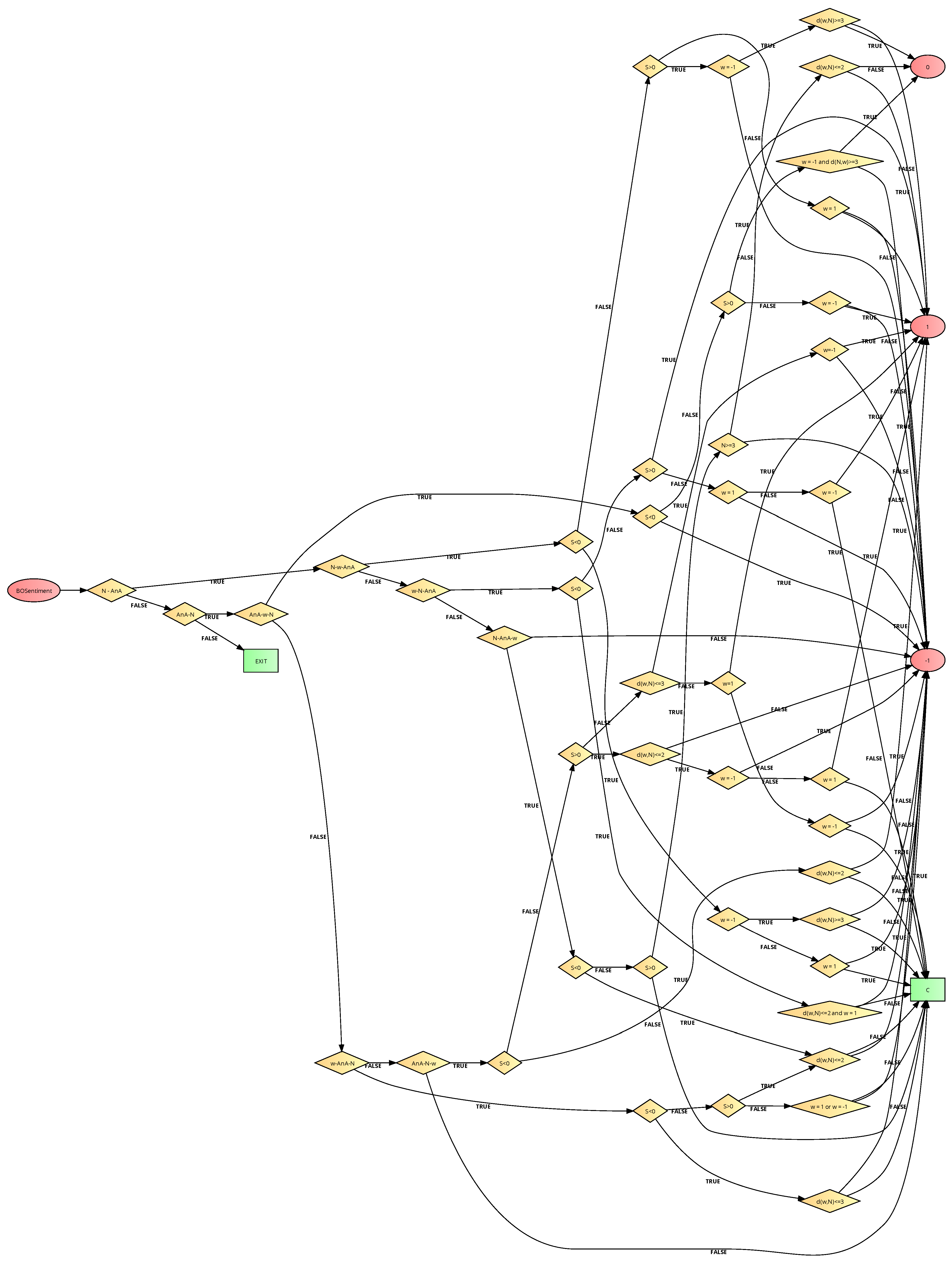
  • The BOSentiment model, which examines the position of negation and AnA-word terms in relation to all other words in the text (see Figure 2).
    Moreover, the BOSentiment classifier works by examining the order of Negation, AnA-words, and lexicon words. In this regard, we have the following possible positions:
    Negation before AnA-words;
    AnA-words before Negation.
    The lexicon word can be found either at the beginning, end, or in the middle between the word from the AnA-words list and Negation.
    The BOSentiment classifier provided in the above Figure checks for these positions and calculates the final sentiment score accordingly.
    The BOSentiment classifier provided in Figure 2 checks for these positions and calculates the final sentiment score accordingly. The sentiment score can be either 1 , 0, or 1, where 1 represents negative sentiment, 0 represents neutral sentiment, and 1 represents positive sentiment. Additionally, at times when we were uncertain about the impact of negation and AnA-words on the sentiment analysis of a tweet, we employed a simple method (1), where all other words that were not labeled as 1 or 1 were labeled with 0. If the resulting value was less than 0, then the tweet was assigned a sentimental value of 1 . Conversely, if the value was greater than 0, the tweet received a sentimental value of 1. If the value was exactly 0, the tweet was deemed to be neutral. This approach was used as a fallback when the more complex analysis involving negation and AnA-words did not produce a clear sentiment value. While not as nuanced as the more sophisticated approach, this simple method still provides a rough estimate of the sentiment of a tweet. The model first checks whether Negation comes before AnA or vice versa. Depending on the order, it then checks the position of the lexicon word to Negation and AnA. If all three elements (Negation, AnA, and lexicon word) are strictly present in a tweet, the classifier then uses the position and relationship between these three elements to determine the final sentiment value. The code follows a set of conditions to determine the sentiment score. For example, if Negation comes before the AnA-words word, the lexicon word is found between Negation and AnA, and the sentiment value of the tweet is negative, the classifier assigns a sentiment score of 1 . Similarly, if AnA comes before Negation, the lexicon word is found at the beginning, and the sentiment value is positive, the classifier assigns a sentiment score of 1. In addition, it includes various conditions that check for the position and relationship between Negation, AnA-words word, and the lexicon word, and assigns the sentiment score accordingly. If any of the three elements are missing in a tweet, the classifier assigns an exit code.
In the initial phase, we gathered a corpus of 11,461 tweets composed in the Bosnian language. Subsequently, we filtered this data-set and pinpointed a specific subset of 417 tweets (238 negatives, 112 neutral, and 67 positives) that exhibited the presence of both negation clues and terms from the AnA-words list.
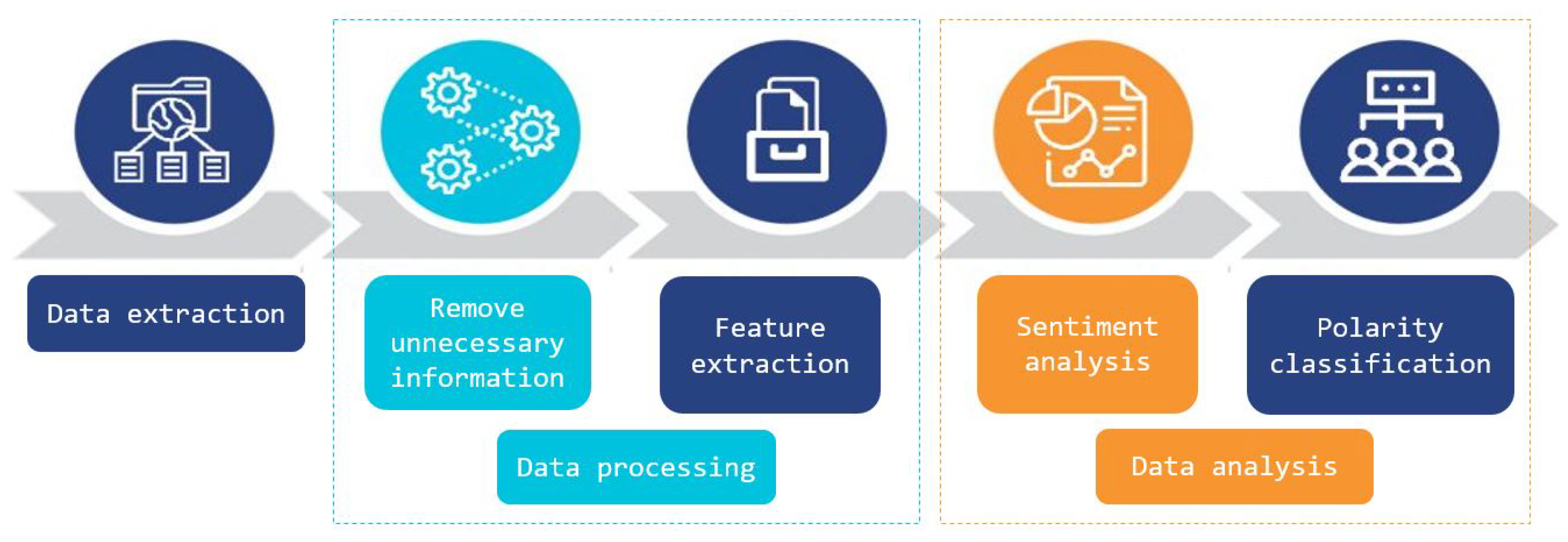
To prepare the data for sentiment analysis, we conducted several tasks. Firstly, we performed cleaning operations, which involved removing unnecessary symbols such as hashtags (#) and mentions (@), as well as eliminating punctuation marks such as quotes, exclamation marks, and hyperlinks. Additionally, we conducted feature extraction to further enhance the data (see Figure 3). For feature extraction, we utilized the Natural Language Toolkit (NLTK) [77] to isolate individual words from each tweet.
Next, we implemented a methodology to assign a categorization label to each word in the tweets. The categorization label represents the classification or category assigned to a word based on its attributes or characteristics. In our case, we assigned a categorization label to each word of the tweet, as depicted in Figure 4. Specifically, negation words were assigned the categorization label N, indicating their role as negations. Words from the AnA-words list were assigned the categorization label AnA. Additionally, as it was proposed by Nitika et al. [27], words from a negative list of lexicon were assigned a label of 1 , indicating a negative sentiment, while words from the positive list of lexicon were assigned a label of 1, indicating a positive sentiment.
With these categorization labels assigned to the words of the tweets, we proceed with the classification of the polarity of each tweet as positive, negative, or neutral.
To achieve this, a methodology inspired by the approach presented in Lexicon-Based Approach to Sentiment Analysis of Tweets Using R Language [27] was implemented. It is based on the tagging method for lexemes with dictionary lookups. The authors evaluated the method on the classification of tweets (as positive or negative). The following formula was used:
Score = Pos ( x , p o s w o r d ) Neg ( x , n e g w o r d ) ,
where x is a phrase, p o s w o r d is a positive word, and n e g w o r d is a negative word.
Based on their method for determining the sentiment value of the text, we utilized our algorithm and calculated the sentiment values ( s e n t i m e n t i ) of tweets as follows:
( i ( 0 , N ) ) : s e n t i m e n t i = j = 0 n v a l u e s j l e n g t h ( t w e e t i ) , N = number of tweets
where v a l u e s j ( j ( 0 , n ) ) , n number of elements in a tweet after processing, are values of a word matched with the lexicon; if it is a positive word, then the score is + 1 , if negative, then the score is 1 , otherwise, 0.
In this way, we have restricted the values so that s e n t i m e n t i in our case ranges from [ 1 , 1 ] , where values below 0 represent a negative sentiment, above zero represent a positive sentiment, or neutral if the sentiment value is equal to zero.
In addition to the methodology described above, we also considered the presence of negation clues and terms from the AnA-words list in our sentiment analysis. We included all 6 types of intensifiers [70,71], or 3 types as described by [47], in one group of Affirmative and non-Affirmative words (AnA-words). Jahić and Vičič in [42,75] pointed out that the list of AnA-words consists of 102 words, mostly adverbs.
Depending on the type of intensifier used, they can either diminish or boost the sentiment expressed by the accompanying word. Minimizers or diminishers decrease the sentiment value, while boosters or maximizers increase it [74].
Taboda et al. in [28] pointed out that intensifiers were incorporated into text labeling in such a way that each intensifier was assigned a percentage of its strength. The used formula to embed the intensifier into text labeling is given:
s e n t i m e n t _ v a l u e = s e n t i m e n t _ w o r d + a m p l i f i e r _ p e r c e n t a g e
If multiple amplifiers are given, then the sentiment_value are multiplied. This indicates that the sentiment value of the text is unbounded, meaning that if multiple amplifiers are present in the same text, the resulting sentiment value can become quite large due to the multiplication factor in their calculation formula.
The consideration of negation was implemented by shifting toward the opposite polarity by a fixed amount (in their implementation, 4) instead of changing the sign as done by Sauri [78].
So, for example, the word “good” ( + 3 sentiment value) if negated (not good) would have a sentimental value of 3 4 = 1 .
Supported by Horn [68], who argues that negation can significantly alter the sentiment conveyed by a word or expression, Taboada et al. [28] propose a method where, if a negative expression is encountered in the text, the final sentiment value assigned to that word is increased by 50 % , as in the example:
She’s not good (3 − 4 = −1) but not terrible (−5 + 4 = −1) either.
(Without modifiers and before applying an increase in value by 50%)
She’s not very good (5 ∗ (100% + 25%) − 4 = −0.25 + 50%(−0.25)) but not too terrible (−5 + 4 = −1 + 50%(−1)) either.
(After the application of their method for enhancing the sentiment by 50%)
Given that it is not entirely clear from the presented work how the final sentiment value for a given text was calculated, we assume that a small epsilon was used (In mathematics, a small positive infinitesimal quantity, usually denoted ϵ , whose limit is usually taken as ϵ 0 [79]) value of around 0. In this way, if the final value is less than 0, the sentiment value of the entire text is negative; if the final value is greater than 0, the sentiment value of the entire text is positive; otherwise, it is neutral.)
This means that, in the previous examples, we have the following values:
  • In the first case, the final sentiment value (without modifiers) is 2 , which means that this text is classified as negative.
  • In the second case, the final sentiment value for the given text (with modifiers and applying a shift of 50 % in the case of negation) is 1.875 , which means that this text is also classified as negative.
According to this, we have created a formula that included the effect of intensifiers, in our case, the AnA-words list, in the equation below. Assume that we have N tweets (length greater or equal to two) that are labeled. The counter is a list of numbers of AnA-words for each tweet.
Then, ( i ( 0 , N ) ) :
X i = 0 , s e n t i m e n t i = ± 1 0 c o u n t e r i l e n g t h ( t e x t i ) ( 1 s e n t i m e n t i ) , o t h e r w i s e
the sentiment is given by:
s e n t i m e n t X i = s e n t i m e n t i + X i , s e n t i m e n t i ( 0 , 1 ) s e n t i m e n t i X i , s e n t i m e n t i ( 1 , 0 ) s e n t i m e n t i , s e n t i m e n t i = { 1 , 0 , 1 }
In previous works on sentiment analysis, the effects of intensifiers and negation on the sentiment value of text were not given enough attention. To address this issue, we focused on analyzing terms in which AnA-words and negation appeared together.
Specifically, we labeled tweets based on two models, described in Section 3:
  • The BoSA model, which considers the presence of negation and lexicon terms in the sentence;
  • The BOSentiment model, which examines the position of negation and AnA-words terms in relation to all other words in the text.
Moreover, we have calculated the impact of the BOSentiment model in a convolution neural network (CNN) on the overall determining sentiment value of the data. In that case, we have created two new models:
  • CNN (as a pure neural network model) and
  • CNNBOSentiment model as a model that combines the BOSentiment model as a pre-model and CNN network as a main model to predict sentiment values.
Since our data-set included sentiment data (negative = 1 , positive = 1 , and neutral = 0), we encoded each sentence with three labels, with one value representing the actual label. For instance, “Negative” was represented as [ 1 , 0 , 0 ] , “Neutral” as [ 0 , 1 , 0 ] , and “Positive” as [ 0 , 0 , 1 ] . We used the Tokenizer (https://www.tensorflow.org/api_docs/python/tf/keras/preprocessing/text/Tokenizer (accessed on 1 June 2023) ) and pad_ sequences (https://www.tensorflow.org/api_docs/python/tf/keras/utils/pad_sequences (accessed on 1 June 2023)) functions from Keras’ preprocessing module to transform the text data into sequences of integers. The Tokenizer function is used to convert the text data into a numerical format by mapping each word in the text to a unique integer value. The pad_sequences function ensures that each sequence has the same length by padding the sequences with zeros or truncating them to a fixed length.
As can be seen from Listing 1, we used seven layers in our model:
  • Embedding maps each word to a 32-dimensional vector. The number 5000 represents the total number of words in the vocabulary, and input_length represents the maximum length of input sequences that will be processed. In this case, the maximum sequence length is set to 32.
  • Conv1D performs convolution on the input sequence using filters of size 5 × 32 . The number 64 represents the number of filters used in the layer, and ‘ReLu’ indicates the activation function Rectified Linear Unit (ReLU) that is applied after convolution.
  • MaxPooling1D with pool_size is 4 were applied after Conv1D layer. MaxPooling1D applies maxpooling operation to each feature dimension of the 3D input tensor (batch_size, steps, features), where steps represent the length of the sequence and features represent the number of features in each step. The pool_size is 4 means that the operation will pool four adjacent values at a time and return the maximum value of those four. This reduces the length of the sequence by a factor of 4 while retaining the most important features. The output of MaxPooling1D is a 3D tensor with shape (batch_size, new_steps, features), where new_steps is the result of dividing the original steps by the pool_size (rounded down).
  • Flatten was applied after MaxPoolong1D layer. This layer flattens the input data into a one-dimensional array. In other words, it takes the 3D tensor output from the previous layer and converts it into a 1D array that can be used as input to a fully connected (Dense) layer. The output shape of the Flatten layer is a 1D tensor with a length equal to the product of the dimensions of the input tensor (batch_size, steps, features).
Listing 1. CNN model with 7 layers.
model = Sequential()
model.add(Embedding(5000, 32, input_length=maxlen))
model.add(Conv1D(64, 5, activation=‘relu’))
model.add(MaxPooling1D(pool_size=4))
model.add(Flatten())
model.add(Dense(64, activation=‘relu’))
model.add(Dropout(0.4))
model.add(Dense(3, activation=‘softmax’))
Then, two Dense layers were applied. The reason for using Dense layers is to perform classification on the features extracted by the previous convolutional layers. After the feature maps have been flattened into a 1D array, Dense layers are added to the model to learn non-linear relationships between the features and the target variable.
  • 1st Dense has 64 neurons and uses the ReLU (Rectified Linear Unit - a simple and computationally efficient function that returns the input value if it is positive, and 0 otherwise) activation function. It transforms the flattened feature vector into a new vector of length 64. This allows the model to learn more complex representations of the features.
  • Dropout is a technique used in neural networks to prevent over-fitting. During training, the Dropout layer randomly selects some of the neurons and “drops” them, meaning they will be ignored during that particular forward and backward pass. This forces the remaining neurons to learn more robust features that are relevant to the classification task. The probability of dropping a neuron is a hyper-parameter and is usually set to a value between 0.2 and 0.5 .
  • 2nd Dense has 3 neurons and uses the softmax (The output of the softmax activation function can be interpreted as the predicted probability of each class, and the predicted class is simply the one with the highest probability.) activation function. It takes the output of the previous layer and maps it to a probability distribution over the three classes—positive, negative, or neutral. This allows the model to make a prediction on which class the input sequence belongs to.
In the second model CNN+BOSentiment (ID: CNNBOSentiment), first, we transformed the text data and labels into a format that can be input into a neural network for training and prediction. If we are using BOSentiment as a pre-predicted model, then negation cues were mapped as [ 0 , 1 , 0 , 0 , 0 ] , negative words as [ 1 , 0 , 0 , 0 , 0 ] , neutral words as [ 0 , 0 , 0 , 0 , 0 ] , AnA-words as [ 0 , 0 , 0 , 1 , 0 ] , and positive words as [ 0 , 0 , 0 , 0 , 1 ] .
For this model, we used 6 layers:
  • Conv2D adds a 2D convolutional layer with 32 filters of size 3 × 3. The activation function used is ReLU;
  • MaxPooling2D((2,2)) adds a max pooling layer that reduces the spatial dimensions of the output of the previous layer. The ( 2 , 2 ) parameter specifies the size of the pooling window. In this case, the layer pools the maximum value of a 2 × 2 window in the output.
  • Flatten() adds a flattened layer that converts the output of the previous layer to a 1D array. This is necessary because the next layer in the model is a dense layer that requires a 1D input.
The last three layers were the same as for the CNN model:
  • 1st Dense ( Dense ( 64 , activation = relu ) ),
  • Dropout (Dropout ( 0.4 ) ),
  • 2nd Dense (Dense (3, activation=‘softmax’)).
In this section, we describe the methodology and work we conducted to evaluate the performance of different classifiers for sentiment analysis on our data-set. We tested models with and without the use of the BOSentiment model and compared their performance using accuracy, precision, recall, and F 1 score metrics.
Furthermore, we examined the effect of different parameter values on the accuracy of our convolutional neural networks, and an overview is given in Table 1.
Table 1 showcases models created based on varying numbers of convolutional layers, filters, their sizes, number of epochs, and batch sizes. The models are divided into two sections: CNN (Convolutional Neural Network) and CNNBOSentiment. In the CNNBOSentiment section, models combining CNN with the BOSentiment model are presented, while the CNN section represents pure CNN models with different utilized layers.

4. Results

This section presents a comparison of several algorithms for the sentiment classification of textual data. All the algorithms were presented in Section 3. The performance of these algorithms was analyzed on the provided data-set, which contains three classes (negative, neutral, and positive). The aim was to evaluate how well the algorithms can classify tweets into one of these three classes. The used evaluation metrics [80] were precision, recall, and F 1 score and accuracy score [81] as performance measures. We also used the hamming loss metric [82] to assess how well the algorithms can handle multi-class classification. The confusion matrix [83] was used as a visual representation of the evaluation of the performance of the models.
In Table 2 there are several measures used to evaluate classifier performance -precision, recall, F 1 score, accuracy, and the Hamming loss score.
The Table 2 shows the classification report for various classifiers based on their precision, F 1 score, mean squared error ( σ M ), standard deviation ( σ ), and Hamming loss. Each classifier is listed with its corresponding precision score for each class ( 1 , 0 , 1 ) and the F 1 score. The σ M and σ values indicate the classifier’s error and dispersion, respectively, while the Hamming loss measures the fraction of unclassified labels.
The best-performing classifier according to the table is BOSentiment with the highest precision score for all classes and the highest F 1 score of 0.89 . It also has the lowest σ M and σ values, indicating the smallest error and dispersion, respectively. Additionally, it has the lowest Hamming loss of 0.11 , indicating the smallest fraction of unclassified labels. Overall, BOSentiment is the most accurate and precise classifier among the listed options.
Looking at the table, we can see that the next best classifier after BOSentiment is BoSA, which has a precision score of 0.78 and a relatively low Hamming loss of 0.22 . BoSA has the highest precision scores for each sentiment label, and its F 1 score is also relatively high compared to the other classifiers. However, it has a higher mean squared error and standard deviation compared to BOSentiment, indicating a higher amount of error and variance in its predictions.
The next best classifiers after BoSA are Decision Tree and k-Nearest Neighbors, both with precision scores of around 0.5 and a Hamming loss of 0.32 . Decision Tree has higher precision scores for negative and neutral sentiment, while k-Nearest Neighbors has higher precision scores for positive sentiment.
Bernoulli Naive Bayes and Random Forest have similar precision scores of around 0.57–0.58 and a relatively high Hamming loss of 0.43 and 0.32 , respectively. Bernoulli Naive Bayes has the highest precision score for positive sentiment, while Random Forest has the highest precision scores for negative and neutral sentiment.
Multinomial Naive Bayes and Complements Naive Bayes have the lowest precision scores among the classifiers listed in the table, both with a precision score of around 0.38 and a Hamming loss of 0.43 . Complements Naive Bayes has the highest precision score for positive sentiment, while Multinomial Naive Bayes has the highest precision score for neutral sentiment.
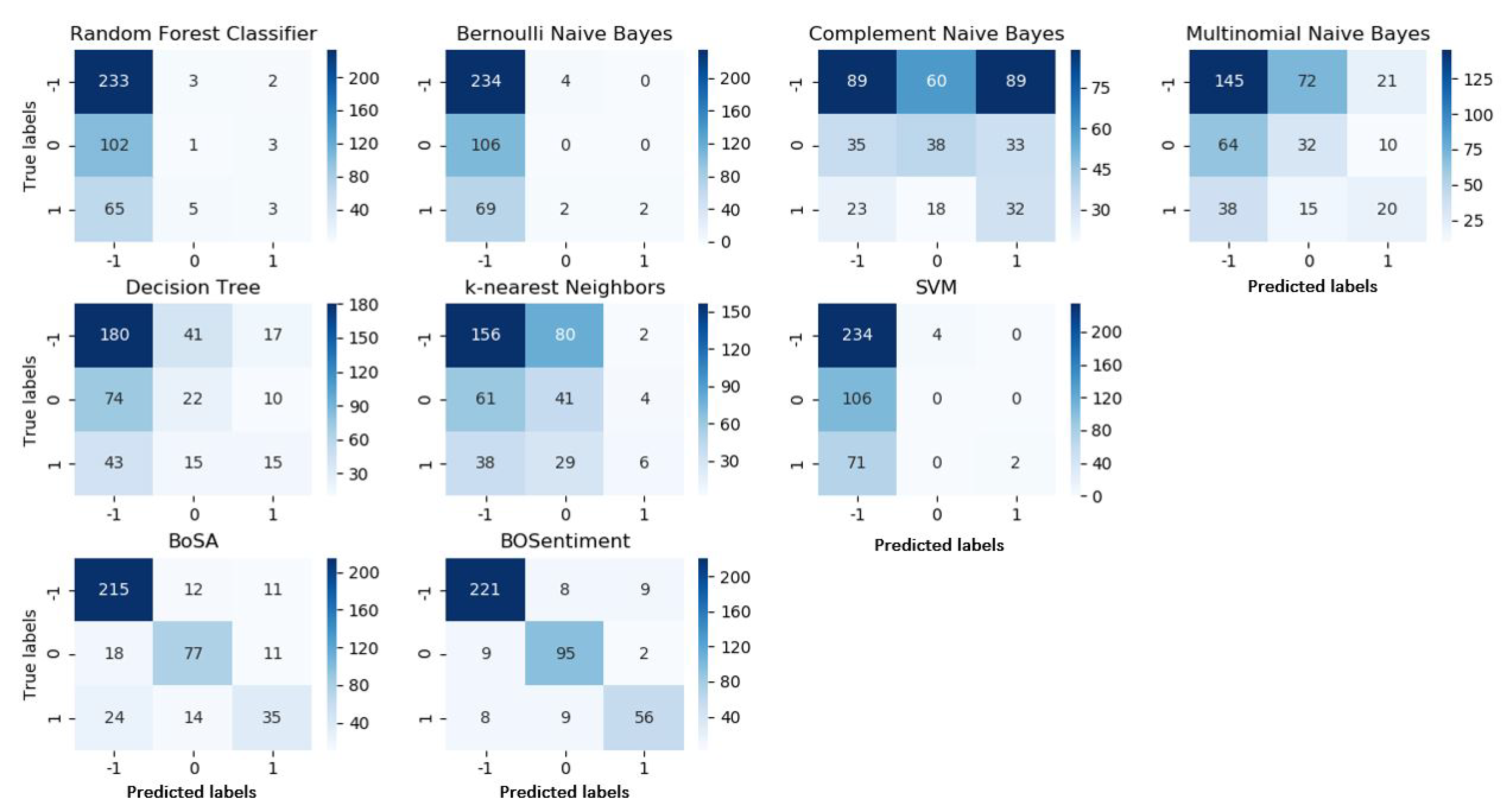
Moreover, to clarify the good performance of BOSentiment and BoSA, we have also calculated the confusion matrix (A confusion matrix is a tool used to evaluate the performance of a classification model. It shows the number of correct and incorrect predictions made by the model compared to the actual outcomes. The matrix is usually represented as a table where each row represents the true labels and each column represents the predicted labels.).
Looking at the confusion matrices provided in Figure 5, we can see that the diagonal elements of the matrix (the true positive predictions) have higher values compared to the off-diagonal elements (the false positive and false negative predictions). This indicates that the models performed well in correctly identifying the true class labels.
For example, in the case of the BoSA classifier, we can see that the diagonal elements have high values, particularly for the first and second classes (represented in the rows and columns). This suggests that the model was able to correctly classify a large number of instances belonging to these classes. However, we can also see that there are some misclassifications, particularly in the third class, which may require further investigation.
Similarly, for the BOSentiment classifier, we see high values along the diagonal elements for the first and third classes. This indicates that the model was successful in correctly predicting a large number of instances belonging to these classes. However, there are some misclassifications in the second class, which may require further investigation.
Overall, the confusion matrices provide valuable insights into the performance of the classification models and can help guide further improvements to the models.
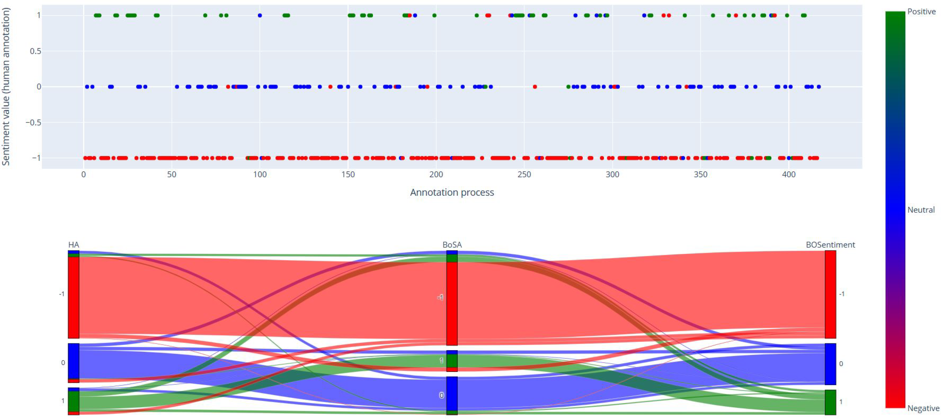
Having that in mind, we conducted an overall annotation using the BOSentiment model, which was processed with the BoSA model. First, we used the BoSA model to extract the sentiment values of the tweets. Then, those values were used as features for the BOSentiment model. As can be seen from the lower part of Figure 6, the left side consists of a number of tweets that were labeled by humans (238 negatives, 106 neutrals, and 73 positives). By processing these tweets with the BoSA model, we calculated the sentiment values of the tweets, and we got correctly classified 215 negative tweets, 77 neutral tweets, and 35 positive tweets. Those sentiment values were then processed with the BOSentiment model which gave us correctly classified 221 negative tweets, 95 neutral tweets, and 56 positive tweets.
On the top of Figure 6 in the scatter can be seen a comparison between human annotation and the BOSentiment model.
Moreover, as can be seen from Table 3, we have 92.86 % negative tweets that were correctly classified as negative with the BOSentiment classifier, 89.62 % that remained neutral after classification, and 76.71 % that were classified correctly as positive.
In order to further reinforce the accuracy of our model, we utilized Neural Networks, specifically Convolution neural networks (CNN).
As mentioned earlier, our data-set included sentiment data (negative, positive, and neutral), so, we encoded each sentence with three labels, with one value representing the actual label. For instance, “Negative” was represented as [ 1 , 0 , 0 ] , “Neutral” as [ 0 , 1 , 0 ] , and “Positive” as [ 0 , 0 , 1 ] .
As can be seen from Listing 1, we have used seven layers in our pure CNN model.
After applying Embedding and the Conv1D layer, we get a new matrix of dimensions ( 3 , 28 , 64 ) . This matrix is obtained by interpreting our initial matrix of dimensions ( 3 , 32 ) as 3 rows, each of length 32, and then applying a filter of dimensions ( 5 , 32 ) on each of these rows using 64 filters. Each filter takes 5 consecutive vectors of length 32 and applies a convolution operation that generates a single number, resulting in a matrix of dimensions ( 3 , 28 , 64 ) that contains the output of each filter for each row of the initial matrix.
After applying the MaxPooling1D layer, we get a new matrix of dimensions ( 3 , 7 , 64 ) . This matrix is obtained by applying a pooling operation of dimensions ( 4 , ) on each of the 28 elements of each row from the previous Conv1D layer.
This operation takes the maximum value from each group of 4 adjacent elements, reducing dimensionality and resulting in a new matrix of dimensions ( 3 , 7 , 64 ) .
Then, the Flatten layer was applied, which gave us a vector of length 1344 ( 1344 = 3 × 7 × 64 ) . This layer converts the 3D matrix ( 3 , 7 , 64 ) into a 1D vector of length 1344. This means that each element of this vector will contain the value of one of the 64 filters for each of the three sequences.
After that, two Dense layers were applied. The reason for using Dense layers is to perform classification on the features extracted by the previous convolutional layers. After the feature maps have been flattened into a 1D array, Dense layers are added to the model to learn non-linear relationships between the features and the target variable.
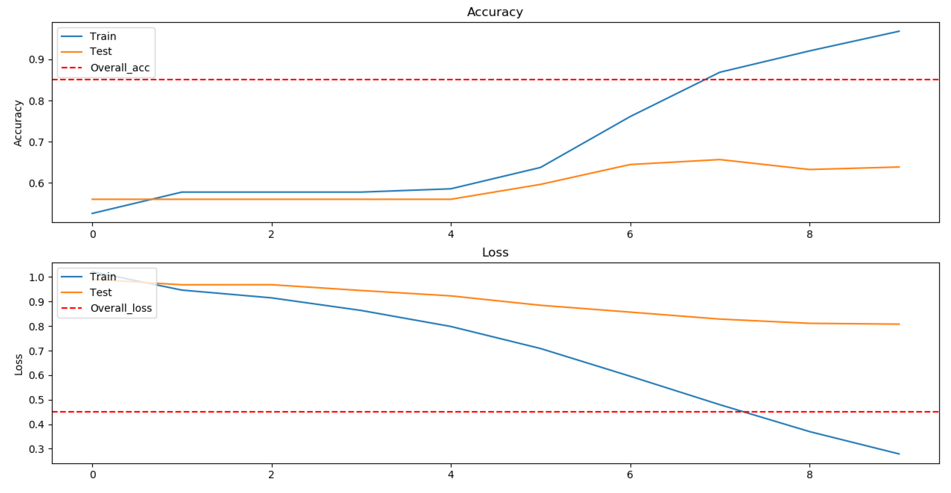
Overall, we obtained that accuracy, in this case, is just over 86.09 % (see Figure 7).
In the second model CNNBOSentiment, first, we transformed the text data and labels into a format that could be input into a neural network for training and prediction. If we were using BOSentiment as a pre-predicted model, then negation cues were mapped as [ 0 , 1 , 0 , 0 , 0 ] , negative words as [ 1 , 0 , 0 , 0 , 0 ] , neutral words as [ 0 , 0 , 0 , 0 , 0 ] , AnA-words as [ 0 , 0 , 0 , 1 , 0 ] , and positive words as [ 0 , 0 , 0 , 0 , 1 ] .
For this model, we used 6 layers (as was already described in Section 3), where the last three layers were the same as for the CNN model.
The BOSentiment model performed well on its own in predicting sentiment for tweets. However, when combined with the CNN model as a pre-predicted model, the results did not show a significant improvement in accuracy when the training data was over 40 % . Table 4 provides the training and testing accuracy for both CNN and CNNBOSentiment models under different training data percentages. We can see that the CNNBOSentiment model had a higher accuracy than the CNN model in both training and testing, but the difference was not significant when the split data on training and testing was 40:60. This suggests that using the BOSentiment model as a pre-predicted model may not be necessary when the training data is sufficient, and the CNN model alone may be enough to achieve good performance.
Having that in mind, we wanted to prove that different parameters can impact the accuracy of the two given models: CNN and CNNBOSentiment. So, we examined the effect of different parameter values on the accuracy of our convolutional neural networks. Basically, we created 20 different models for sentiment annotation (see Table 1), and splitting of the data-set on train and test was 70 : 30 .
In Table 5, we present an evaluation of the performance of 20 CNN models used for text classification. The table shows the training and testing results of these models on the data-set.
The performance criteria of the models were evaluated using the accuracy and loss measures during training and testing.
From Table 5, we can see that the models have different performances. For example, ‘CNN1’ has the highest accuracy on the training set but has relatively low accuracy on the testing set. On the other hand, ‘CNN1e12’ has the best accuracy on the testing set but has relatively low accuracy on the training set. This suggests that the ‘CNN1e12’ model is more generalized and performs better in unknown situations.
On another side, when the BOSentiment model is combined with CNN we can see that there are at least two models that reach better accuracy than the base model BOSentiment (see Table 2).
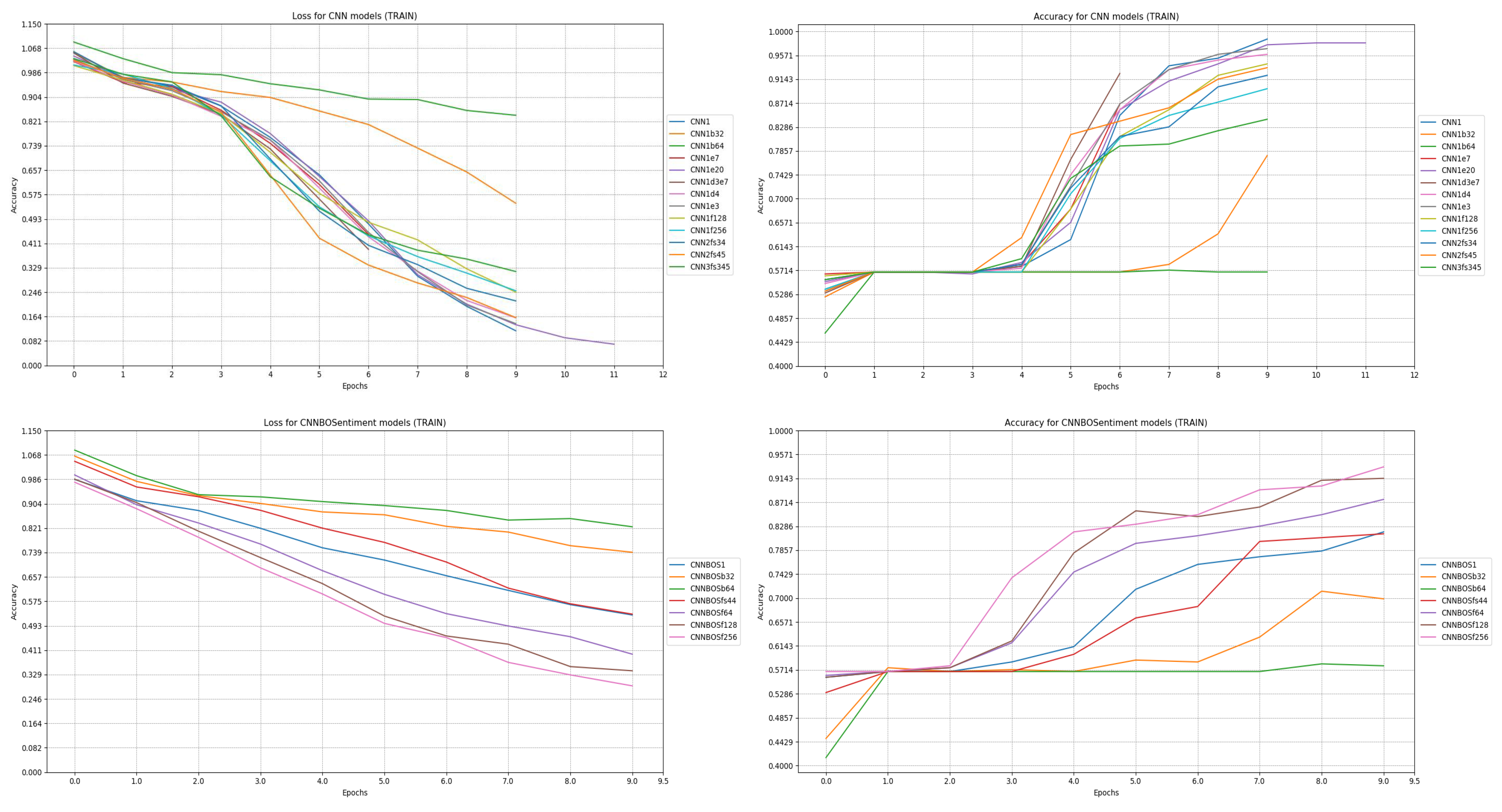
Moreover, a graphical representation of these results would further clarify the performance of the models and enable easier comparison of different models. The following Figure 8 shows the performance of the models on the training and testing sets.
Based on the results presented in Table 5 and Figure 8, the ‘CNNBOSf256’ model stands out as the best performer with an accuracy of around 92 % . This means that when combined with the CNN model with 256 filters of size 4 × 4 , BOSentiment outperforms all other models.

5. Discussion and Further Work

Considering the limited research on sentiment analysis in the Bosnian language, the presented models, particularly the BOSentiment model on its own or in combination with CNN, have shown acceptable performance in accurately sentimentally labeling tweets written in Bosnian. This highlights the potential and effectiveness of our models in addressing sentiment analysis tasks in underrepresented languages. Taking all the results into consideration, it is evident that there is substantial performance variability across the different models, and there is no universal solution. However, based on the outcomes presented in the table and the graph, the ‘CNNBOSf256’ model emerges as the top performer with an accuracy of approximately 92 % . This model surpasses other models, including the widely used CNN models, and achieves a relatively low error. Therefore, based on these findings, we consider the ‘CNNBOSf256’ model to be the most suitable candidate for sentiment classification tasks of the Bosnian language. Even more, the method is easily applicable at least to similar/related languages (at least all the languages from the south-Slavic language group), with possible applications to other languages.
Furthermore, the base model BOSentiment performed well in predicting sentiment for tweets but combining it with CNN as a pre-predicted model did not result in much better accuracy if the training data and testing data were split 40:60, as shown in Table 4. This serves as additional confirmation that the BOSentiment model has a good structure and is an excellent pre-trained model for CNN.
The future focus will be on improving the results of the presented study by upgrading the BOSentiment model and examining AnA-words in separate categories to contribute to better sentiment analysis of the Bosnian language. Additionally, the aim will be to explore the possibility of incorporating context-specific sentiment analysis, such as analyzing tweets based on their source or topic. Furthermore, the performance of other machine-learning algorithms, such as Support Vector Machines, Random Forests, and other neural networks, will be investigated and the results will be compared with those obtained from the current approach. Ultimately, the goal is to provide a more accurate and comprehensive sentiment analysis of the Bosnian language on social media platforms.

Author Contributions

Conceptualization, methodology, software, validation, formal analysis, investigation, resources, original draft preparation, visualization S.J.; review and editing, supervision, funding acquisition J.V. All authors have read and agreed to the published version of the manuscript.

Funding

Funding for this research was provided by European Commission through the Horizon 2020 ‘InnoRenew CoE’ (Grant Agreement no. 739574) and SRC-EDIH—Smart, Resilient, and Sustainable Communities—European Digital Innovation Hub (Grant Agreement no. 101083351).

Institutional Review Board Statement

Not applicable.

Informed Consent Statement

Not applicable.

Data Availability Statement

Not applicable.

Conflicts of Interest

The authors declare no conflict of interest.

Abbreviations

The following abbreviations are used in this manuscript:
AnAA word from the AnA-words list
AnA-wordsAffirmative and non-Affirmative words
BCMSBosnian-Croatian-Montenegrin-Serbian language
BERTBidirectional Encoder Representations from Transformers
CNNConvolution Neural Network
CRFConditional random fields
LBMLexicon-based method
NLTKNatural Language Toolkit
RFRandom Forest
SVMSupport Vector Machine

References

  1. The editors of Encyclopaedia Britannica. Bosnian-Croatian-Montenegrin-Serbian Language Summary. 2021. Available online: https://www.britannica.com/summary/Bosnian-Croatian-Montenegrin-Serbian-language (accessed on 1 June 2023).
  2. Čušić, T. D1.36: Report on the Bosnian Language. 2023. Available online: https://european-language-equality.eu/wp-content/uploads/2022/03/ELE___Deliverable_D1_36__Language_Report_Bosnian_.pdf (accessed on 1 June 2023).
  3. Agency for Statistics of Bosnia and Herzegovina. Cenzus of Population, Households and Dwellings in Bosnia and Herzegovina, 2013 Final Results. 2013. Available online: https://dataspace.princeton.edu/handle/88435/dsp0176537424z (accessed on 1 June 2023).
  4. Pang, B.; Lee, L. Opinion mining and sentiment analysis. Found. Trends Inf. Retr. 2008, 2, 1–135. [Google Scholar] [CrossRef] [Green Version]
  5. Liu, B. Sentiment Analysis and Opinion Mining; Morgan & Claypool Publishers: San Rafael, CA, USA, 2012. [Google Scholar]
  6. Gunasekaran, K.P. Exploring Sentiment Analysis Techniques in Natural Language Processing: A Comprehensive Review. arXiv 2023, arXiv:2305.14842. [Google Scholar]
  7. Vaswani, A.; Shazeer, N.; Parmar, N.; Uszkoreit, J.; Jones, L.; Gomez, A.N.; Kaiser, L.; Polosukhin, I. Attention is All You Need. In Proceedings of the 31st International Conference on Neural Information Processing Systems, Long Beach, CA, USA, 4 December 2017; Curran Associates Inc.: Red Hook, NY, USA, 2017; pp. 6000–6010. [Google Scholar]
  8. Catelli, R.; Pelosi, S.; Esposito, M. Lexicon-based vs. Bert-based sentiment analysis: A comparative study in Italian. Electronics 2022, 11, 374. [Google Scholar] [CrossRef]
  9. Cambria, E.; Hussain, A.; Havasi, C.; Eckl, C. A new approach to sentic computing: Ontology-based representation of natural language semantics. In Proceedings of the IEEE International Conference on Granular Computing, Beijing, China, 13 December 2013; pp. 397–402. [Google Scholar]
  10. Storey, V.C.; O’Leary, D.E. Text analysis of evolving emotions and sentiments in COVID-19 Twitter communication. Cogn. Comput. 2022, 1–24. [Google Scholar] [CrossRef]
  11. Pak, A.; Paroubek, P. Twitter as a corpus for sentiment analysis and opinion mining. In Proceedings of the LREC, Valletta, Malta, 19 May 2010; Volume 10, pp. 1320–1326. [Google Scholar]
  12. Agarwal, A.; Xie, B.; Vovsha, I.; Rambow, O.; Passonneau, R. Sentiment analysis of Twitter data. In Proceedings of the Workshop on Languages in Social Media, Portland, OR, USA, 23 June 2011; Association for Computational Linguistics: Baltimore, MD, USA, 2011; pp. 30–38. [Google Scholar]
  13. Go, A.; Bhayani, R.; Huang, L. Twitter sentiment classification using distant supervision. In Proceedings of the 22nd International Conference on Computational Linguistics-Volume 2; Association for Computational Linguistics: Baltimore, MD, USA, 2009; pp. 1–4. [Google Scholar]
  14. Joachims, T. Text categorization with support vector machines: Learning with many relevant features. In Proceedings of the Machine learning: ECML-98, Chemnitz, Germany, 21 April 1998; Volume 1398, pp. 137–142. [Google Scholar]
  15. Cortes, C.; Vapnik, V. Support-vector networks. Mach. Learn. 1995, 20, 273–297. [Google Scholar] [CrossRef]
  16. Kurani, A.; Doshi, P.; Vakharia, A.; Shah, M. A comprehensive comparative study of artificial neural network (ANN) and support vector machines (SVM) on stock forecasting. Ann. Data Sci. 2023, 10, 183–208. [Google Scholar] [CrossRef]
  17. McCallum, A.; Nigam, K. A comparison of event models for naive Bayes text classification. In Proceedings of the AAAI Conference on Artificial Intelligence, AAAI-98 Workshop on Learning Text Categorization, Madison, WI, USA, 26 July 1998; Volume 752, pp. 41–48. [Google Scholar]
  18. Rish, I. An empirical study of the naive Bayes classifier. In Proceedings of the IJCAI 2001 Workshop on Empirical Methods in Artificial Intelligence, Seattle, WA, USA, 4 August 2001; Volume 3, pp. 41–46. [Google Scholar]
  19. Reddy, E.M.K.; Gurrala, A.; Hasitha, V.B.; Kumar, K.V.R. Introduction to Naive Bayes and a Review on Its Subtypes with Applications. In Bayesian Reasoning and Gaussian Processes for Machine Learning Applications; CRC: Boca Raton, FL, USA, 2022; pp. 1–14. [Google Scholar]
  20. Breiman, L. Random forests. In Proceedings of the Machine Learning; Springer: Berlin/Heidelberg, Germany, 2001; Volume 45-1, pp. 5–32. [Google Scholar]
  21. Wang, F.; Zhang, C.; Liu, X.; Zhang, Y. Sentiment classification based on random forests. Expert Syst. Appl. 2011, 38, 7677–7683. [Google Scholar]
  22. Mardjo, A.; Choksuchat, C. HyVADRF: Hybrid VADER–Random Forest and GWO for Bitcoin Tweet Sentiment Analysis. IEEE Access 2022, 10, 101889–101897. [Google Scholar] [CrossRef]
  23. Kim, Y. Convolutional neural networks for sentence classification. In Proceedings of the Methods in Natural Language Processing (EMNLP), Doha, Qatar, 25 October 2014; pp. 1746–1751. [Google Scholar]
  24. Severyn, A.; Moschitti, A. Twitter sentiment analysis with deep convolutional neural networks. In Proceedings of the 38th International ACM SIGIR Conference on Research and Development in Information Retrieval, Santiago, Chile, 9–13 August 2015; ACM: Hong Kong, China, 2015; pp. 959–962. [Google Scholar]
  25. Wang, L.; Tang, R.; Zhao, S.; Zhang, Y.; Zhang, Y. Sentiment Analysis of Twitter Data: A Comprehensive Study. In Proceedings of the 2020 International Conference on Data Science and Information Technology (DSIT), Xiamen, China, 24 July 2020; pp. 243–248. [Google Scholar]
  26. Pang, B.; Lee, L.; Vaithyanathan, S. Thumbs up? Sentiment Classification using Machine Learning Techniques. In Proceedings of the 2002 Conference on Empirical Methods in Natural Language Processing (EMNLP 2002), Philadelphia, PA, USA, 6 July 2002; Association for Computational Linguistics: Stroudsburg, PA, USA; pp. 79–86. [Google Scholar] [CrossRef] [Green Version]
  27. Nigam, N.; Yadav, D. Lexicon-Based Approach to Sentiment Analysis of Tweets Using R Language. In Proceedings of the ICACDS 2018: Advances in Computing and Data Sciences; Springer: Singapore, 2018; pp. 154–164. [Google Scholar] [CrossRef]
  28. Taboada, M.; Brooke, J.; Tofiloski, M.; Voll, K.; Stede, M. Lexicon-Based Methods for Sentiment Analysis. Comput. Linguist. 2011, 37, 267–307. [Google Scholar] [CrossRef]
  29. Osgood, C.E.; Suci, G.J.; Tannenbaum, P.H. The Measurement of Meaning; University of Illinois Press: Urbana, IL, USA, 1957. [Google Scholar]
  30. Bruce, R.; Wiebe, J. Recognizing Subjectivity: A Case Study of Manual Tagging. Nat. Lang. Eng. 2000, 5, 187–205. [Google Scholar] [CrossRef] [Green Version]
  31. Hu, M.; Liu, B. Mining and Summarizing Customer Reviews. In Proceedings of the Tenth ACM SIGKDD International Conference on Knowledge Discovery and Data Mining, Seattle, WA, USA, 22 August 2004; pp. 168–177. [Google Scholar] [CrossRef] [Green Version]
  32. Kim, S.M.; Hovy, E. Determining the Sentiment of Opinions. In Proceedings of the 20th International Conference on Computational Linguistics, Geneva, Switzerland, 23 August 2004; p. 1367-es. [Google Scholar] [CrossRef]
  33. Stone, P.; Dunphy, D.; Smith, M.; Ogilvie, D. The General Inquirer: A Computer Approach to Content Analysis; The MIT Press: Cambridge, MA, USA, 1966; Volume 4. [Google Scholar] [CrossRef]
  34. Jahić, S.; Vičič, J. Sentiment Polarity Lexicon of Bosnian Language. 2023. Available online: https://zenodo.org/record/7520809 (accessed on 1 June 2023). [CrossRef]
  35. Kapukaranov, B.; Nakov, P. Fine-Grained Sentiment Analysis for Movie Reviews in Bulgarian. In Proceedings of the PInternational Conference Recent Advances in Natural Language Processing, Hissar, Bulgaria, 7 September 2015; pp. 266–274. [Google Scholar]
  36. Glavaš, G.; Šnajder, J.; Dalbelo Bašić, B. Semi-supervised Acquisition of Croatian Sentiment Lexicon. In Proceedings of the International Conference on Text, Speech and Dialogue, Brno, Czech Republic, 3–7 September 2012; Volume 7499, pp. 166–173. [Google Scholar] [CrossRef]
  37. Veselovská, K. Czech Subjectivity Lexicon: A Lexical Resource for Czech Polarity Classification. In Proceedings of the 7th International Conference, Slovko, Bratislava, 4 July 2013; pp. 279–284. [Google Scholar]
  38. Jovanoski, D.; Pachovski, V.; Nakov, P. Sentiment Analysis in Twitter for Macedonian. In Proceedings of the International Conference Recent Advances in Natural Language Processing, Hissar, Bulgaria, 7 September 2015; pp. 249–257. [Google Scholar]
  39. Wawer, A. Extracting emotive patterns for languages with rich morphology. Int. J. Comput. Linguist. Appl. 2012, 3, 11–24. [Google Scholar]
  40. Okruhlica, A. Slovak Sentiment Lexicon Induction in Absence of Labeled Data. Master’s Thesis, Comenius University Bratislava, Bratislava, Slovakia, 2013. [Google Scholar]
  41. Kadunc, K. Določanje Sentimenta Slovenskim Spletnim Komentarjem s Pomočjo Strojnega Učenja; K. Kadunc: Washington, DC, USA, 2016. [Google Scholar]
  42. Jahić, S.; Vičič, J. Determining Sentiment of Tweets Using First Bosnian Lexicon and (AnA)-Affirmative and Non-affirmative Words. In Advanced Technologies, Systems, and Applications V: Papers Selected by the Technical Sciences Division of the Bosnian-Herzegovinian American Academy of Arts and Sciences 2020; Springer International Publishing: Cham, Switzerland, 2021; pp. 361–373. [Google Scholar] [CrossRef]
  43. Jahić, S.; Vičič, J. Annotated lexicon for sentiment analysis in the Bosnian language. In Proceedings of the ALTNLP The International Conference and workshop on Agglutinative Language Technologies as a Challenge of Natural Language Processing, Koper, Slovenia, 7–8 June 2022; Volume 3315, pp. 9–19. [Google Scholar]
  44. Tadić, M.; Brozović-Rončević, D.; Kapetanović, A. The Croatian Language in the Digital Age; Springer: Berlin/Heidelberg, Germany, 2012; p. 93. [Google Scholar]
  45. Pelicon, A.; Pranjić, M.; Miljković, D.; Škrlj, B.; Pollak, S. Sentiment Annotated Dataset of Croatian News. Slovenian Language Resource Repository CLARIN.SI. 2020. Available online: https://www.clarin.si/repository/xmlui/handle/11356/1342 (accessed on 1 June 2023).
  46. Mozetič, I.; Grčar, M.; Smailović, J. Twitter sentiment for 15 European languages, 2016. Slovenian language resource repository CLARIN.SI.
  47. Pavić Pintarić, A.; Frleta, Z. Upwards Intensifiers in the English, German and Croatian Language. J. Foreign Lang. 2014, 6, 31–48. [Google Scholar] [CrossRef]
  48. Krstev, C.; Pavlovic-Lazetic, G.; Vitas, D.; Obradović, I. Using Textual and Lexical Resources in Developing Serbian Wordnet. Rom. J. Inf. Sci. Technol. 2004, 7, 147–161. [Google Scholar]
  49. Mladenovic, M.; Mitrović, J.; Krstev, C.; Vitas, D. Hybrid Sentiment Analysis Framework for a Morphologically Rich Language. J. Intell. Inf. Syst. JIIS 2015, 46, 599–620. [Google Scholar] [CrossRef]
  50. Batanović, V.; Nikolić, B.; Milosavljević, M. Reliable Baselines for Sentiment Analysis in Resource-Limited Languages: The Serbian Movie Review Dataset. In Proceedings of the Tenth International Conference on Language Resources and Evaluation (LREC’16), Portorož, Slovenia, 5 May 2016; pp. 2688–2696. [Google Scholar]
  51. Kovacevic, J.; Graovac, J. Application of a Structural Support Vector Machine method to N-gram based text classification in Serbian. Infotheca J. Digit. Humanit. 2015, 16, 1–2. [Google Scholar] [CrossRef] [Green Version]
  52. Drašković, D.; Zečević, D.; Nikolić, B. Development of a Multilingual Model for Machine Sentiment Analysis in the Serbian Language. Mathematics 2022, 10, 3236. [Google Scholar] [CrossRef]
  53. Ljajić, A.; Stanković, M.; Marovac, U. Detection of Negation in the Serbian Language. In Proceedings of the 8th International Conference on Web Intelligence, Mining and Semantics, New York, NY, USA, 5 July 2018. [Google Scholar] [CrossRef]
  54. Ljajić, A.B. Obrada Negacije u Kratkim Neformalnim Tekstovima u Cilju Poboljšanja Klasifikacije Sentimenta/Processing Negation in Short Informal Text for Improving the Sentiment Classification. Ph.D. Thesis, University of Niš, Niš, Serbia, 2019. [Google Scholar]
  55. Bučar, J.; Žnidaršič, M.; Povh, J. Annotated news corpora and a lexicon for sentiment analysis in Slovene. Lang. Resour. Eval. 2018, 52, 895–919. [Google Scholar] [CrossRef]
  56. Mozetič, I.; Grčar, M.; Smailović, J. Multilingual Twitter Sentiment Classification: The Role of Human Annotators. PLoS ONE 2016, 11, 1–26. [Google Scholar] [CrossRef]
  57. Fišer, D.; Smailović, J.; Erjavec, T.; Mozetič, I.; Grčar, M. Sentiment annotation of Slovene user-generated content. In Proceedings of the Zbornik Konference Jezikovne Tehnologije in Digitalna Humanistika, Ljubljana, Slovenija, 29 September–1 October 2016; Erjavec, T., Fišer, D., Eds.; Znanstvena Založba Filozofske Fakultete = Ljubljana University Press: Ljubljana, Slovenija, 2016. [Google Scholar]
  58. Moilanen, K.; Pulman, S. Sentiment Composition. In Proceedings of the Proceedings of the Recent Advances in Natural Language Processing International Conference (RANLP-2007), Borovets, Bulgaria, 27 September 2007; pp. 378–382. [Google Scholar]
  59. Singh, P.K.; Paul, S. Deep learning approach for negation handling in sentiment analysis. IEEE Access 2021, 9, 102579–102592. [Google Scholar] [CrossRef]
  60. Councill, I.; McDonald, R.; Velikovich, L. What’s great and what’s not: Learning to classify the scope of negation for improved sentiment analysis. In Proceedings of the Workshop on Negation and Speculation in Natural Language Processing, Uppsala, Sweden, 5 September 2010; pp. 51–59. [Google Scholar]
  61. Morante, R.; Daelemans, W. A Metalearning Approach to Processing the Scope of Negation. In Proceedings of the Thirteenth Conference on Computational Natural Language Learning (CoNLL-2009), Boulder, CO, USA, 9 June 2009; pp. 21–29. [Google Scholar]
  62. Reitan, J.; Faret, J.; Gambäck, B.; Bungum, L. Negation Scope Detection for Twitter Sentiment Analysis. In Proceedings of the 6th Workshop on Computational Approaches to Subjectivity, Sentiment and Social Media Analysis, Lisboa, Portugal, 7 September 2015; pp. 99–108. [Google Scholar] [CrossRef] [Green Version]
  63. Jia, L.; Yu, C.; Meng, W. The Effect of Negation on Sentiment Analysis and Retrieval Effectiveness. In Proceedings of the 18th ACM Conference on Information and Knowledge Management, CIKM ’09, Hong Kong, China, 2 November 2009; pp. 1827–1830. [Google Scholar] [CrossRef] [Green Version]
  64. Wiegand, M.; Balahur, A.; Roth, B.; Klakow, D.; Montoyo, A. A survey on the role of negation in sentiment analysis. In Proceedings of the NeSp-NLP@ACL, Uppsala, Sweden, 10 July 2010. [Google Scholar]
  65. Polanyi, L.; Zaenen, A. Contextual Valence Shifters. In Computing Attitude and Affect in Text: Theory and Applications; Springer: Dordrecht, The Netherlands, 2006; pp. 1–10. [Google Scholar] [CrossRef]
  66. Kennedy, A.; Inkpen, D. Sentiment Classification of Movie Reviews Using Contextual Valance Shifters. Comput. Intell. 2006, 22, 110–125. [Google Scholar] [CrossRef] [Green Version]
  67. Zhu, X.; Guo, H.; Mohammad, S.; Kiritchenko, S. An Empirical Study on the Effect of Negation Words on Sentiment. In Proceedings of the 52nd Annual Meeting of the Association for Computational Linguistics (Volume 1: Long Papers), Baltimore, MD, USA, 6 June 2014; pp. 304–313. [Google Scholar] [CrossRef] [Green Version]
  68. Horn, L.R. A Natural History of Negation; University of Chicago Press: Chicago, IL, USA, 1989. [Google Scholar]
  69. Wilson, T.; Wiebe, J.; Hoffmann, P. Recognizing Contextual Polarity in Phrase-Level Sentiment Analysis. In Proceedings of the Human Language Technology Conference and Conference on Empirical Methods in Natural Language Processing, Vancouver, BC, Canada, 7 October 2005; pp. 347–354. [Google Scholar]
  70. Merima, O. A Contribution to the Classification of Intensifiers in English and Bosnian. In Književni Jezik 21/2; Institut za Jezik: Sarajevo, Bosnia and Herzegovina, 2003; pp. 50–62. [Google Scholar]
  71. Patra, B.; Mazumdar, S.; Das, D.; Rosso, P.; Bandyopadhyay, S. A Multilevel Approach to Sentiment Analysis of Figurative Language in Twitter. In Proceedings of the Computational Linguistics and Intelligent Text Processing, Konya, Turkey, 3 April 2018; Springer International Publishing: Berlin/Heidelberg, Germany, 2018; pp. 281–291. [Google Scholar]
  72. Kennedy, G. Amplifier Collocations in the British National Corpus: Implications for English Language Teaching. TESOL Q. 2003, 37, 467–487. [Google Scholar] [CrossRef]
  73. Recski, L. “… It’s Really Ultimately Very Cruel …”: Contrasting English intensifier collocations across EFL writing and academic spoken discourse. DELTA Doc. Estud. Lingüística Teórica Apl. 2004, 20, 211–234. [Google Scholar] [CrossRef] [Green Version]
  74. Quirk, R.; Greenbaum, S.; Leech, G.; Svartvik, J. A Comprehensive Grammar of the English Language; Longman: London, UK, 1985. [Google Scholar]
  75. Jahić, S.; Vičič, J. The Lists of AnAwords and Stopwords are Publicly Available on the Zenodo Repository. 2023. Available online: https://zenodo.org/record/8021150 (accessed on 1 June 2023). [CrossRef]
  76. Ljajić, A.; Marovac, U. Improving sentiment analysis for twitter data by handling negation rules in the Serbian language. Comput. Sci. Inf. Syst. 2019, 16, 289–311. [Google Scholar] [CrossRef] [Green Version]
  77. Bird, S.; Klein, E.; Loper, E. Natural Language Processing with Python: Analyzing Text with the Natural Language Toolkit; O’Reilly Media, Inc.: Newton, MA, USA, 2009. [Google Scholar]
  78. Sauri, R. A Factuality Profiler for Eventualities in Text. Ph.D. Thesis, Brandeis University, Brandeis, MA, USA, 2008. [Google Scholar]
  79. Derbyshire, J. (Ed.) Prime Obsession: Bernhard Riemann and the Greatest Unsolved Problem in Mathematics; The National Academies Press: Washington, DC, USA, 2003. [Google Scholar] [CrossRef]
  80. Hossin, M.; Sulaiman, M.N. A Review on Evaluation Metrics for Data Classification Evaluations. Int. J. Data Min. Knowl. Manag. Process. 2015, 5, 1–11. [Google Scholar] [CrossRef]
  81. Pedregosa, F.; Varoquaux, G.; Gramfort, A.; Michel, V.; Thirion, B.; Grisel, O.; Blondel, M.; Prettenhofer, P.; Weiss, R.; Dubourg, V.; et al. Scikit-learn: Machine Learning in Python. J. Mach. Learn. Res. 2011, 12, 2825–2830. [Google Scholar]
  82. Madjarov, G.; Kocev, D.; Gjorgjevikj, D.; Džeroski, S. An extensive experimental comparison of methods for multi-label learning. Pattern Recognit. 2012, 45, 3084–3104. [Google Scholar] [CrossRef]
  83. Ting, K.M. Confusion Matrix. In Encyclopedia of Machine Learning; Springer: Boston, MA, USA, 2010; p. 209. [Google Scholar] [CrossRef]
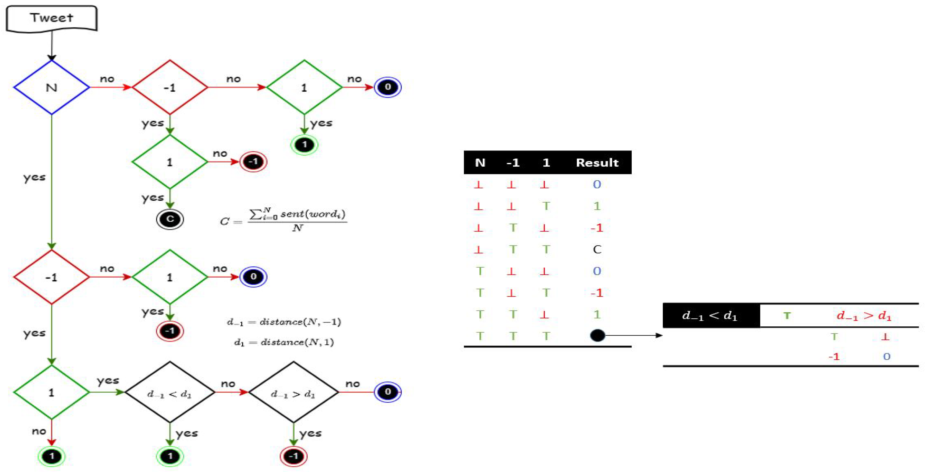
Figure 1. BoSA model for the classification of the tweets.
Applsci 13 07760 g001
Figure 2. BOSentiment model for the classification of the tweets.
Applsci 13 07760 g002
Figure 3. Data processing for sentiment analysis.
Applsci 13 07760 g003
Figure 4. The classification or category assigned to a term based on its attributes or characteristics.
Applsci 13 07760 g004
Figure 5. Visualization of the performance of algorithms in the confusion matrix. The output matrix has six cells, diagonal elements present a number of elements that were classified as correct for the given sentiment value, and all other presents a number of elements that were not classified as correct.
Applsci 13 07760 g005
Figure 6. Annotation of the tweets with the BOSentiment model through the BoSa model. The BoSA model was used to extract the sentiment values of the tweets, which were used as features for the BOSentiment model.
Applsci 13 07760 g006
Figure 7. Loss and accuracy plot for the pure CNN model. The model achieved an accuracy score of 86.09 % for the test:train split of 30:70, indicating its effectiveness in classifying the data. The loss curve shows a decreasing trend, indicating that the model was able to learn and improve its predictions over time.
Applsci 13 07760 g007
Figure 8. Performance of 20 CNN models on training and testing data. The CNN model with 256 filters of size 4 × 4 stands out as the best performer with an accuracy of around 92 % .
Applsci 13 07760 g008
Table 1. An overview of the convolutional neural network (CNN) models and CNN models with the BOSentiment model. Models were created based on different numbers of convolutional layers, filters, and their sizes, epochs, and batch size.
ID_ModelShort ID[cl a ][f b ][fs c ][d d ][e e][b f ]
CNN
cnn_cl1_f64-fs5_d5_e10_b16CNN116450.51016
cnn_cl1_f64-fs5_d5_e10_b32CNN1b3216450.51032
cnn_cl1_f64-fs5_d5_e10_b64CNN1b6416450.51064
cnn_cl1_f64-fs5_d5_e7_b16CNN1e716450.5716
cnn_cl1_f64-fs5_d5_e12_b16CNN1e1216450.51216
cnn_cl1_f64-fs5_d3_e7_b16CNN1d3e716450.3716
cnn_cl1_f64-fs5_d4_e10_b16CNN1d416450.41016
cnn_cl1_f64-fs3_d4_e10_b16CNN1e316430.41016
cnn_cl1_f128-fs3_d4_e10_b16CNN1f128112830.41016
cnn_cl1_f256-fs3_d4_e10_b16CNN1f256125630.41016
cnn_cl2_f64-fs34_d4_e10_b16CNN2f342643, 40.41016
cnn_cl2_f64-fs45_d4_e10_b16CNN2f452644, 50.41016
cnn_cl3_f64-fs345_d4_e10_b16CNN3f3453643, 4, 50.41016
CNNBOSentiment
cnnBOS_cl1_f32_fs33_d4_e10_b16CNNBOS11323 × 30.41016
cnnBOS_cl1_f32_fs33_d4_e10_b32CNNBOSb321323 × 30.41032
cnnBOS_cl1_f32_fs33_d4_e10_b64CNNBOSb641323 × 30.41064
cnnBOS_cl1_f32_fs44_d4_e10_b16CNNBOSfs441324 × 40.41016
cnnBOS_cl1_f64_fs44_d4_e10_b16CNNBOSf641644 × 40.41016
cnnBOS_cl1_f128_fs44_d4_e10_b16CNNBOSf12811284 × 40.41016
cnnBOS_cl1_f256_fs44_d4_e10_b16CNNBOSf25612564 × 40.41016
a : Number of convolution layers. b : Number of filters. c : Filters size. d : Dropout. e: Number of epochs. f : Batch size.
Table 2. Performance comparison of different classifiers for tweet classification. BoSA and BOSentiment achieve the highest F 1 score for all sentiment instances ( 1 , 0 , 1 ) and have the highest accuracy scores. Additionally, BOSentiment outperforms BoSA with a higher accuracy score.
ClassifierPrecisionRecall F 1 Score
(Class)
Avg. F 1 Score
(Model)
Accuracy
Score
σ M a σ b Hamming Loss
Score
Random Forest−10.580.980.730.440.580.250.320.32
00.250.010.02
10.500.070.12
Bernoulli Naive Bayes−10.570.980.720.420.570.880.180.43
00.000.000.00
11.000.030.05
Complements NB−10.610.370.460.400.380.370.850.43
00.330.360.34
10.210.440.28
Multinomial NB−10.590.610.600.470.470.330.700.43
00.270.300.28
10.390.270.32
Decision Tree−10.610.710.660.490.520.370.710.32
00.340.280.31
10.300.220.25
k-Nearest Neighbors−10.610.660.630.470.490.780.550.32
00.270.390.32
10.500.080.14
SVM−10.570.980.720.420.570.350.170.35
00.000.000.00
11.000.030.05
BoSA−10.840.900.870.780.780.470.720.22
00.750.730.74
10.610.480.54
BOSentiment−10.930.930.930.890.890.230.750.11
00.850.900.87
10.840.770.80
a : Mean squared error on whole data. b : Standard deviation on whole data.
Table 3. Cross-tabulation for Human Annotation and BOSentiment model. Truly correctly classified tweets are given on the main diagonal.
BOSentiment
NegativeNeutralPositiveTotal
Negative22189238
Human AnnotationNeutral9952106
Positive895673
Total23811267417
Table 4. Accuracy scores for sentiment prediction models across different data splits.
ModelTraining accTesting acc
(40:60)
30:7020:80
CNN0.63860.79380.86090.9376
CNNBOSentiment0.73490.81530.80820.8345
Table 5. Summary of CNN and CNNBOSentiment models’ training and testing metrics. ‘CNN1’ achieves the highest training accuracy, while ‘CNN1e12’ exhibits the highest testing accuracy. The superior performance of ‘CNN1e12’ on the testing set suggests its better generalization ability.
ModelTrain LossTrain AccuracyTest LossTest Accuracy
CNN
CNN10.11650.98630.88280.6480
CNN1b320.54570.77740.58680.8273
CNN1b640.84200.56850.83460.5707
CNN1e70.44130.86990.47500.8465
CNN1e120.07150.97950.35560.8801
CNN1d3e70.39050.92470.44770.8801
CNN1d40.16020.95890.32220.8633
CNN1e30.14050.96920.32870.8585
CNN1f1280.24650.94180.40950.8753
CNN1f2560.25110.89730.45300.8633
CNN2fs340.21710.92120.59860.8417
CNN2fs450.16080.93490.53010.8537
CNN3fs3450.31600.84251.06630.7314
CNNBOSentiment
CNNBOS10.52900.81850.55240.8273
CNNBOSb320.74010.69860.71280.7002
CNNBOSb640.82600.57880.81330.5731
CNNBOSfs440.53190.81510.51670.8345
CNNBOSf640.39720.87670.46930.8681
CNNBOSf1280.34120.91440.39810.8969
CNNBOSf2560.29050.93490.35130.9137
Disclaimer/Publisher’s Note: The statements, opinions and data contained in all publications are solely those of the individual author(s) and contributor(s) and not of MDPI and/or the editor(s). MDPI and/or the editor(s) disclaim responsibility for any injury to people or property resulting from any ideas, methods, instructions or products referred to in the content.