Abstract
In cattle breeding, regularly taking the animals to the scale and recording their weight is important for both the performance of the enterprise and the health of the animals. This process, which must be carried out in businesses, is a difficult task. For this reason, it is often not performed regularly or not performed at all. In this study, we attempted to estimate the weights of cattle by using stereo vision and semantic segmentation methods used in the field of computer vision together. Images of 85 animals were taken from different angles with a stereo setup consisting of two identical cameras. The distances of the animals to the camera plane were calculated by stereo distance calculation, and the areas covered by the animals in the images were determined by semantic segmentation methods. Then, using all these data, different artificial neural network models were trained. As a result of the study, it was revealed that when stereo vision and semantic segmentation methods are used together, live animal weights can be predicted successfully.
1. Introduction
Livestock farming has become an important industrial sector as well as a side occupation for people engaged in agriculture in rural areas. Thanks to practices such as cooperatives, producer unions, registered breeding, artificial insemination practices, and livestock supports, the place of the livestock sector in the country’s economy has started to gain more importance. It is necessary to determine the weight of the animals raised in cattle breeding farms and to follow them regularly. Increasing the profitability of the business depends on the regular follow-up of live weight [1].
The most common method of measuring the live weight of farm animals is traditional measurement using a scale. Although this direct approach is very accurate, it comes with various difficulties and limitations. Firstly, animals are required to be moved to the site of measurement scale, which can be time-consuming and laborious, especially in farms with a large number of animals. Secondly, this whole operation with the separation of animals from their natural environment causes stress, and therefore negatively affects their health and milk yield. Due to those drawbacks of direct measurement approaches, a variety of indirect measurement approaches have been proposed in the literature [2]. In indirect measurement, the true value of animal live weight is estimated by a regression model trained on various features extracted from measurements obtained from several sensors such as 2D [3] and 3D cameras [4], thermal cameras [5], and ultrasonic sensors [6].
In this study, we consider the determination of the live weight of farm animals as a computer vision and a regression problem. First, we obtain the images of farm animals using a stereo setup. Then, applying deep learning-based semantic segmentation techniques, we extract distance and size data from images to feed into a regression model. Finally, we obtain the weight estimates from the regression model as a proxy for the actual weights of the animals. The main motivation for our study was to apply state-of-the-art image processing techniques using modern deep learning approaches to propose an effective solution to the problem considered. The main contributions and novelty of our study can be summarized as follows:
- We propose an effective indirect measurement method for determining the live weight of farm animals based on stereo vision and state-of-the-art semantic segmentation techniques using deep learning.
- Our method is particularly important in that animals’ body measurements are taken without the need for separating them from their natural environments and thus not adversely affecting their health and milk yield.
- We propose a very simple yet effective system and setup composed of relatively cheaper hardware that is accessible and affordable for many farms of small to large scale.
- We investigate and compare the performances of three different Artificial Neural Network (ANN) architectures in estimating live animal weight.
2. Related Work
In this section, we provide essential background on livestock weight estimation with a review of significant past research. Our focus in this review is on the work with indirect measurement approaches based on image processing techniques. We also summarize them in Table 1.

Table 1.
Summary of the previous studies.
There are several studies in the literature that are based on image processing techniques on 2D images. In a study by Weber et al., the live body weight of cattle was estimated using dorsal area images taken from above using a kind of fence system [7]. Their system first performs segmentation and then generates a convex hull around the segmented area to obtain features to feed a Random Forest-based regression model. Tasdemir and Ozkan performed a study where they predicted the live weight of cows using an ANN-based regression model [8]. They determined various body dimensions such as wither height, hip height, body length, and hip width applying photogrammetric techniques on images of cows captured from various angles. Wang et al. developed an image processing-based system to estimate the body weight of pigs [9]. Their main approach was to process images captured from above to extract features such as area, convex area, perimeter, and so on. Then, using these features, they trained an ANN-based regression model for weight prediction. A Fuzzy Rule-Based System was also utilized in cattle weight estimation by Anifah and Haryanto [10]. They obtained 2D side images of cattle from a very close distance of 1.5 m. After applying the Gabor filter to the images, they obtained body length and circumference as features. Finally, they designed a fuzzy logic system to estimate body weight.
Three-dimensional imaging techniques also found application in body weight estimation systems. Hansen et al. used a 3D Kinect-like depth camera to obtain the views of cows from above as they passed along a fence [11]. Applying thresholding, they obtained the segmented area of cows to reach a body weight estimate. In another study where a 3D Kinect camera was used, Fernandes et al. processed images taken from above of pigs by applying two segmentation steps [12]. Then, they extracted features from segmented images such as body area, volume, width, and height to feed a linear regression model to obtain the weight estimate. In a similar study, Cominotte et al. developed a system to capture images of cattle using a 3D Kinect camera [13]. They trained and compared a number of linear and non-linear regression models by feeding them with features extracted from segmented images. In a study by Martins et al., a 3D Kinect camera was used to capture images of cows from lateral and dorsal perspectives [14]. They used several measurements obtained from these images to run a Lasso regression model to estimate body weight. Nir et al. used a 3D Kinect camera as well to take images of dairy heifers to estimate height and body mass [15]. Their approach was to fit an ellipse to the body image to calculate some features. Then, they used these features to train various linear regression models. Song et al. created a system to estimate the body weight of cows using a 3D camera system [16]. Similar to previous studies, they extracted morphological features from 3D images such as hip height, hip width, and rump length. Combining these features with some other cow data such as days in milk, age, and parity, they trained multiple linear regression models. Another study that employed a 3D Kinect camera is the one conducted by Pezzuolo et al. [17]. They captured body images of pigs using two cameras from top and side, and then extracted body dimensions from images such as heart girth, length, and height using image processing techniques. They developed linear and non-linear regression models based on these dimensions to predict weight.
Advanced scanning devices were also introduced in body weight estimation studies. Le Cozler et al. used a 3D full-body scanning device to obtain very detailed body images of cows [18]. Then, they computed body measures from these 3D images such as volume, area, and other morphological traits. Using these measures, they trained and compared several regression models. Stajnko et al. developed a system to make use of thermal camera images of cows to extract body features and then used them in several linear regression models to estimate body weight [19].
Stereo vision techniques are also used in the determination of live animal weight. Shi et al. developed a regression model to analyze and estimate the body size and live weight of farm pigs under indoor conditions in a farm [20]. Their system was based on a binocular stereo vision system and a special fence system through which animals passed for taking the measurements. They segmented the images obtained from the stereo system using a depth threshold and predicted the body length and withers height, then the body weight. Some other notable studies using stereo vision are by Nishide et al. and Yamashita et al. [21,22].
Deep learning-based approaches are very popular today due to their success in image-processing applications. Deep learning is a special form of neural network algorithm. Although it has achieved the most advanced results in many fields, its use in determining the weight of livestock is limited [23]. There are studies that apply deep learning algorithms and determine the weight of pigs [24,25].
When we examine the prior research on the estimation of live body weight of farm animals such as pigs, cattle, cows, and heifers, there is a common approach to capturing images of animals that the animals are forced to move into special types of boxes or fences, or they are forced to pass through a special passage. This operation is very similar to traditional weight measurement with scales, and therefore, it also requires the separation of animals from their natural environment, and it causes stress-related problems in their health and milk yield [3]. Our proposed approach is superior to this in that animals’ pictures are taken in their natural environments without the need for a special measurement station. Additionally, our approach is totally contactless and pictures do not need to be taken from very close proximity, unlike previous studies. One other advantage of our proposed approach provides a simpler structure and setup composed of relatively cheaper hardware that can be accessible and affordable for many farms of small to large scale. Last but not least, we employ modern and state-of-the-art deep learning-based image processing techniques in our system, which is one of the few such studies.
3. Materials and Methods
3.1. Overview of the Proposed Method
Our proposed system is composed of a number of steps performing various tasks from raw data collection to model training. These steps are presented in Figure 1 as block components and they are described in their respective subsections.
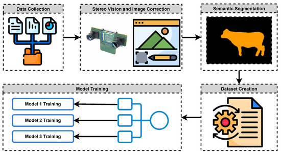
Figure 1.
General block diagram of the study.
3.2. Data Collection
In the study, a stereo setup was prepared to obtain animal images. The stereo mechanism is used to capture digital images with stereo vision techniques used in computer vision and to obtain some inferences from these images. The setup used in the study is shown in Figure 2.
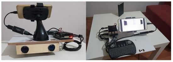
Figure 2.
The stereo vision mechanism used in the study.
During the data collection phase, 85 animals were photographed from the side and the back with this setup. In total, 170 pairs and 340 stereo images were obtained. Using stereo vision techniques on these images, the distance of each animal to the camera plane was calculated.
Architectural components of the stereo setup are given in Figure 2 and their relationships are presented in Figure 3. At the heart of the system is a Raspberry Pi 4 microcomputer with 4 GB of RAM, where the Python code we developed runs to capture animal images. It is powered by a mobile power supply. Two Microsoft Lifecam Studio Webcams are connected to it via two USB ports. A mobile phone with Android OS acts as a monitor and it is connected to Raspberry Pi via Video Capture USB 2.0 to HDMI converter. Finally, a wireless mini integrated keyboard and touchpad are used to control the device.

Figure 3.
Architectural components of the stereo setup.
3.3. Stereo Vision and Image Correction
Stereo vision is a technique used to calculate the distance and position of a point to the camera plane viewed by two cameras whose relative positions and projections are known. A single camera is a mapping between a 3D world and a 2D image [26,27,28]. The geometry of a stereo setup consisting of two identical cameras is shown in Figure 4.

Figure 4.
Diagram of stereo camera system.
Here, and Or are the focal points of both cameras, f is the focal length of both cameras, P is any point in space, Z is the distance of this point in space to the camera plane, T is the translation value between the two cameras. and are reflections of the P point on both viewing planes. This geometry creates similar triangles between the and points. The Z value can be easily calculated using Equation (1) and the similarity theorem.
In Figure 4, the – value is expressed with the variable d. In stereo vision, the d value is also expressed as disparity. In order to increase the accuracy of the stereo vision calculation, stereo calibration is required. Stereo calibration is related to the rotation matrix R, which defines the relative rotation between the coordinate systems of the two cameras, and the transformation vector T, which defines the translation of the two camera centers. After a correctly performed calibration, R and T matrices are obtained. By using the calibration matrices obtained as a result of stereo calibration, corrections or rectification processes can be made on stereo images. Stereo rectification ensures that objects are positioned correctly in pairs of images to match the stereo arrangement. Thus, the stereo distance calculation is performed with less cost and higher accuracy. Stereo rectification aligns the image pair for more reliable stereo distance results [28]. Example images obtained with the help of stereo setup are shown in Figure 5.
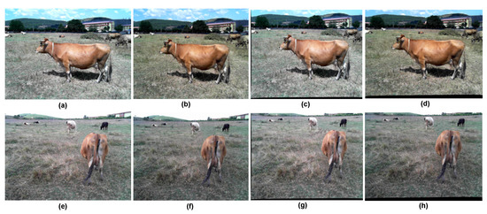
Figure 5.
Rectified and unrectified stereo images: (a,e) Original image taken from left camera. (b,f) Original image taken from right camera. (c,g) Rectified left camera view. (d,h) Rectified right camera view.
3.4. Deep Learning and Semantic Segmentation
Deep learning, a sub-branch of machine learning, is used in many different fields. Deep learning algorithms offer better results than traditional machine learning algorithms if more data are provided. Therefore, object segmentation approaches such as Mask R-CNN [29] based on deep learning can also be used to perform tasks such as weight estimation. Semantic segmentation is used to determine object boundaries. In this study, deep learning semantic segmentation methods were used on stereo images, and then the areas covered by the animals in the images were determined. Semantic segmentation classifies each pixel in the image as belonging to a class. Various models have been introduced in semantic segmentation over time: the Fully Convolutional Network [30], which is based on deep learning; U-Net [31], which takes its name from its architecture and is used especially in medical problems; and Deeplab v3+ [32], which showed the highest success in segmentation tasks in the PASCAL VOC 2012 dataset in 2018. In this study, the PASCAL VOC 2012 dataset and Deeplab v3+ segmentation model were used to perform segmentation tasks on the rectified images. Deeplab v3+ architecture is shown in Figure 6.
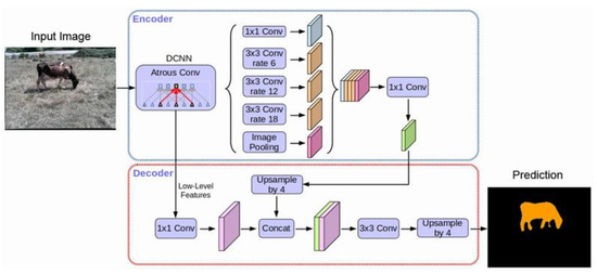
Figure 6.
Deeplab v3+ Architecture.
The segmentation results on the images taken with the model used are shown in Figure 7 and Figure 8.
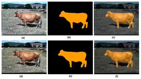
Figure 7.
Segmentation results in stereo images taken from the side: (a) Left camera input image; (b) Left camera segmentation map; (c) Left camera segmentation overlay; (d) Right camera input image; (e) Right camera segmentation map; (f) Right camera segmentation overlay.
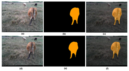
Figure 8.
Segmentation results in stereo images taken from the rear: (a) Left camera input image; (b) Left camera segmentation map; (c) Left camera segmentation overlay; (d) Right camera input image; (e) Right camera segmentation map; (f) Right camera segmentation overlay.
3.5. Dataset Creation
After completing the segmentation processes in all images, the number of pixels occupied by the animals was calculated in the segmentation maps of the images from the left and right cameras for each animal. The distance of each animal to the camera plane was calculated by stereo calculation technique using segmentation maps. In order to calculate the distance of the animal to the camera plane from the segmentation maps, the position of the left border of the animal in pixels on the X-axis was determined in each of the image pairs. The disparity (d) value was calculated by subtracting the limit value in the segmentation map from the left camera and the limit value in the segmentation map coming from the right camera. Figure 9 shows the pixel numbers of the areas covered by a sample animal in the stereo image pair and the X-axis value of the left border of the animal in both images.

Figure 9.
Disparity value and pixels count of the animal in the image: (a) Left camera segmentation map; (b) Right camera segmentation map.
The stereo distance calculation for a single animal is conducted as follows. As seen in Figure 9, if the (Left camera view) and (Right camera view) values are subtracted from each other, the disparity (d) value is found as 23 pixels. Along with this value, the distance value can be easily calculated using the focal length (f) from the stereo calibration matrices and the shift value (T) between the cameras from the translation matrix. As a result of the camera calibration processes, the focal length distance was obtained as 646.45 cm. The translation T value for our setup is 9.92 cm. The stereo distance calculation for the example animal in Figure 8 was obtained as in Equation (2).
After calculating the distance values for each animal, the number of pixels occupied by the animals in the images was also determined. Using all these values, a dataset consisting of 85 rows was created for a total of 85 animals. The created dataset is shown in Table 2 and Table 3, and the distances are written in meters.
Table 2.
Dataset created using semantic segmentation and stereo images.
Table 3.
Dataset created using semantic segmentation and stereo images (cont.)
3.6. Model Training
In the images obtained, the number of pixels in the area occupied by the animal, that is, the segmentation data, does not make any sense on its own. Even if an animal is light in weight, it will take up a lot of space in the image if it is viewed close to the plane of the camera. The opposite is also possible. Pixel numbers are directly proportional to weight, and disparity value is inversely proportional to weight. An increase in the disparity value means that the animal is viewed from a point close to the camera plane. In the study, distance-related errors are eliminated, since the stereo camera setup is calibrated. In the images obtained, the values were made meaningful by considering the stereo distance variable. When the prepared dataset is examined, it is seen that there are data at very different scales from each other. While the pixel numbers in the image are expressed in thousands, the stereo distances are expressed in a few meters, and the disparity values are expressed in the range of 5 and 30 pixels. Training a neural network with such inputs may take a lot of time and the network may not be successful enough. Data at such different scales should be expressed as values close to each other by normalization techniques. The main reason for this is that these features are multiplied by the model weights. Data normalization also accelerates the training time by transforming the raw data into a specific range. Data normalization is extremely useful for modeling applications where the inputs are often at very different scales [33]. In this study, the Z-score normalization technique was used. Here, the Z-score value is calculated by Equation (3), where represents the arithmetic mean of the data, standard deviation, and the data to be normalized.
In the study, three different artificial neural networks were trained after the data obtained from the images taken from different directions were normalized. The first network (ANN-1) is trained with image data taken from the side, the second network (ANN-2) from the back, and the third network (ANN-3) from both directions. A total of 90% of the dataset is reserved for training artificial neural networks and 10% for testing. The architecture of artificial neural networks used in the proposed system is shown in Table 4.
Table 4.
Properties of artificial neural networks used in the proposed system.
ANN-1 and ANN-2 artificial neural networks used for training are fully connected networks with a three-element input layer, two hidden layers consisting of 64 nodes, and an output layer consisting of one element. Each network has 4488 parameters. The ReLU function is used as the activation function, the mean absolute error function is used as the loss function, the Adam optimizer is used as the optimizer, and a constant value of is used as the learning rate value. A total of 1000 training steps were seen as sufficient. The ANN-3 network has the same features as other networks. It covers the entire dataset. Therefore, the number of inputs is 8 and the total number of parameters is 4818.
3.7. Recommended Method for Weight Prediction
The performed study is a hybrid system that makes weight estimation using semantic segmentation and stereo distance data together. The basic operation steps of this system for weight predictions are shown in Figure 10.
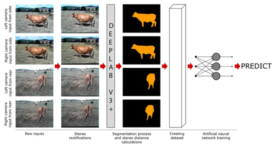
Figure 10.
Basic Operation Steps for Weight Prediction.
4. Results
In this section, we present the prediction performances of the neural networks trained in a comparative manner. The performance levels of the networks are shown in Figure 11.
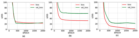
Figure 11.
Loss graphs of artificial neural networks: (a) Loss graph of ANN-1 network; (b) Loss graph of ANN-2 network; (c) Loss graph of ANN-3 network.
The success rate of the ANN-1 network is higher than the ANN-2 network. The reason for this is the inability of the images taken from the back to reveal the general body dimensions of the animal. On the other hand, the performance rate of the ANN-3 network is higher than the other two networks. This is because the network was trained with data from images taken from both angles of animals. Randomly, 10% of the taken images were not used in the training but in the testing of the estimated animal weights. Weight estimation was made separately for the three proposed networks and the results are shown in Table 5, Table 6 and Table 7.
Table 5.
Prediction values on the test dataset of ANN-1 network.
Table 6.
Prediction values on the test dataset of ANN-2 network.
Table 7.
Prediction values on the test dataset of ANN-3 network.
As seen in Table 5, the estimations for the test data made by the ANN-1 network vary between approximately ±50 kg. Note that ANN-1 is only trained with data obtained from the side. In Table 6, the error amounts in the estimations made by the ANN-2 network, which was trained only with photographs taken from the back, vary between approximately ±50 kg. However, the error rates increased dramatically in animals with id numbers 36, 70, and 81. This significantly reduces the accuracy of the network trained with images taken from behind. The reason for this is the inability of the images taken from the back to reveal the general body dimensions of the animal. Table 7 shows the results obtained from the ANN-3 network trained with the entire dataset. In most cases, the predictions were made with a margin of error of approximately ±20 kg, and much more successful results were obtained than the first two networks. The animal image taken in prediction number 36 with a high amount of error is very close to the camera plane. The image of the animal taken very close to the camera plane causes serious errors as it cannot be adequately represented in the dataset. For this reason, it would be more appropriate to take the images to be obtained at reasonable distances not very close to the camera plane.
In this study, the K-fold cross-validation technique was used to test the validity of the proposed method and the accuracy of the results obtained. K-fold cross-validation is one of the methods of splitting the dataset for evaluation of classification models and training of the model [34,35]. This method is used to generate random layers. Each layer represents a combination of training data subset and test data subset sections for training and validating machine learning models. For each layer, a certain accuracy value is obtained for the model. For example, in the case of 10-fold cross-validation, the overall accuracy is estimated by averaging the accuracy values produced by all 10 folds. For any dataset with a given number of samples, there are many possible combinations of training and test datasets that can be generated. Some of these datasets are used to train the model and some are used to test the success of the model. Therefore, it allows each divided part to be used separately for both training and testing. The representation of the K-fold cross-validation method for K = 10 is given in Figure 12.
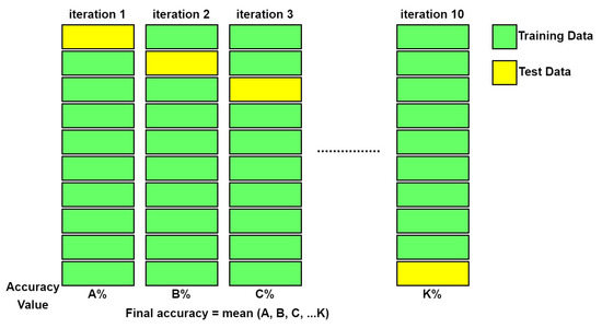
Figure 12.
General structure of the k-fold cross-validation method.
Training and testing the model up to K can take a long time and can be costly in terms of computation and time for large datasets. On the other hand, it provides a reliable result. In this study, the K value was accepted as 10, and validity tests were carried out. Here, the test and training images at each step are meaningfully segmented. A similar situation was repeated at each K step and validity tests were performed on different images. In this study, the validity of the ANN-3 architecture, which was trained using both side and rear images, was tested with K-fold. The results obtained are given in Figure 12. When the predicted values obtained in each K step are compared with the actual values in Table 8, it can be concluded that the proposed model is quite successful. It is thought that 85 animals are not enough to successfully train a neural network. In addition, the weight distribution of the animals, whose images were taken with the stereo device, is generally around 400 kg. Therefore, the estimates made by nets are generally more successful for animals weighing 400 kg. Another weakness of the dataset we created is that animal images are generally taken from 6 to 8 m away. During the image acquisition phase, it was mostly not possible to take images from closer distances, such as 2–3 m, due to frightening the animals. At these distances, stereo vision works more successfully than at distances of 6–8 m. Utilizing all this information, more successful results can be obtained from a trained network with more animal images whose weights are normally distributed. In order to train a neural network successfully, the dataset on which the neural network is trained must be large enough, that is, it must consist of a sufficient number of observations [36]. All known possible variations of the problem area should be added to the dataset. Adequate data delivery to a system is necessary to obtain a robust and reliable network [37,38]. For example, the generated third neural network is trained with data created with images taken from both the side and the back. The amount of error in the weight estimations made by this neural network decreased to the range of ±20 kg.
Table 8.
Example of a table showing that its caption is as wide as the table itself and justified.
5. Discussion
In this study, an attempt was made to estimate live animal weight by using stereo vision and semantic segmentation methods in the literature. Within the scope of the study, a stereo vision device was prepared, and stereo images of 85 cattle whose weights were known beforehand were obtained with this setup. Segmentation maps of the animals in these images were created with the Deeplab v3+ deep learning model, which is one of the semantic segmentation models.
Using the segmentation maps, the number of pixels covered by each animal in the image and their distance to the camera plane were calculated using the stereo distance calculation technique. A dataset was created by combining these obtained data. The dataset was created from the data obtained from photographs of animals taken from two different angles, from the side, and from the back.
Using this dataset, three different artificial neural networks, which are architecturally similar to each other, are trained. When the trained neural networks were compared, it was seen that the third neural network trained with the whole dataset was significantly more successful than the first two neural networks. At this point, it is clear that neural networks to be trained with datasets created with images taken from more angles will be more successful. For example, top images of cattle contain important information about the animal’s body structure. It can be said that networks trained with a dataset that includes top-shot data, if possible, will be more successful.
In addition, it is possible to say that neural networks will make more successful predictions if the quality and quantity of the dataset are increased. In the resulting estimations, although rare, dramatically incorrect estimations were observed. Weight estimations of animals that were limited in number in the dataset, that were light in weight, and whose stereo distance was very different from the rest of the dataset were found to be relatively unsuccessful. Therefore, it is clear that creating a more comprehensive and homogeneously distributed dataset will significantly increase the performance of the models.
Moreover, characteristics such as race and gender of animals directly affect their weight. For example, if the body sizes of two animals of different breeds are assumed to be exactly the same, it will be seen that the weights of these two animals are different from each other. At this point, in the study, a deep learning method that recognizes the breed and gender of the animal can be developed and the performance in weight estimation can be increased with a separate training model for each breed.
6. Conclusions
In this study, we considered the problem of live weight prediction of farm animals from a computer vision perspective. We applied state-of-the-art stereo vision and deep learning-based semantic segmentation using the setup we created that consists of a Raspberry Pi 4 microcomputer and two identical cameras. We used this setup to capture images of 85 farm animals taken from different angles. Applying stereo distance computation and semantic segmentation, we created a dataset to train various ANN models. Our test results of the trained ANNs suggest that our proposed system achieves good performance in terms of weight prediction. The most significant feature of the system is that it does not require the separation of animals from their natural environment to measure their weight, unlike traditional systems. This is particularly important because the separation is known to cause stress and negatively affect health and milk yield. Therefore, our system provides a convenient and contact-free weight measurement with minimal measurement error. The main limitation of our study is the number of images captured from real farm environments. It would be possible to achieve more accurate measurement predictions if more data were available and ANNs were trained with more data.
Funding
This research received no external funding.
Institutional Review Board Statement
Not applicable.
Informed Consent Statement
Not applicable.
Data Availability Statement
Data can be obtained from the corresponding author upon reasonable request.
Acknowledgments
I would like to thank Volkan Tunali for his invaluable suggestions for the research.
Conflicts of Interest
The author declares no conflict of interest.
References
- Kaya, M. Laktasyondaki Holştayn Ineklerde Canlı Ağırlık ve Beden Kondisyon Skorunun Sayısal Görüntü Analizi Yöntemi ile Belirlenebilirliği. Ph.D. Thesis, Aydın Adnan Menderes University, Aydın, Turkey, 2019. [Google Scholar]
- Dang, C.; Choi, T.; Lee, S.; Lee, S.; Alam, M.; Park, M.; Han, S.; Lee, J.; Hoang, D. Machine Learning-Based Live Weight Estimation for Hanwoo Cow. Sustainability 2022, 14, 12661. [Google Scholar] [CrossRef]
- Wang, Z.; Shadpour, S.; Chan, E.; Rotondo, V.; Wood, K.M.; Tulpan, D. ASAS-NANP SYMPOSIUM: Applications of machine learning for livestock body weight prediction from digital images. J. Anim. Sci. 2021, 99, skab022. [Google Scholar] [CrossRef] [PubMed]
- Na, M.H.; Cho, W.H.; Kim, S.K.; Na, I.S. Automatic weight prediction system for Korean cattle using Bayesian ridge algorithm on RGB-D image. Electronics 2022, 11, 1663. [Google Scholar] [CrossRef]
- Vindis, P.; Brus, M.; Stajnko, D.; Janzekovic, M. Non invasive weighing of live cattle by thermal image analysis. In New Trends in Technologies: Control, Management, Computational Intelligence and Network Systems; IntechOpen: London, UK, 2010. [Google Scholar]
- Wang, Q. A Body Measurement Method Based on the Ultrasonic Sensor. In Proceedings of the 2018 IEEE International Conference on Computer and Communication Engineering Technology (CCET), Beijing, China, 18–20 August 2018; pp. 168–171. [Google Scholar]
- Weber, V.A.M.; de Lima Weber, F.; da Silva Oliveira, A.; Astolfi, G.; Menezes, G.V.; de Andrade Porto, J.V.; Rezende, F.P.C.; de Moraes, P.H.; Matsubara, E.T.; Mateus, R.G.; et al. Cattle weight estimation using active contour models and regression trees Bagging. Comput. Electron. Agric. 2020, 179, 105804. [Google Scholar] [CrossRef]
- Tasdemir, S.; Ozkan, I.A. ANN approach for estimation of cow weight depending on photogrammetric body dimensions. Int. J. Eng. Geosci. 2019, 4, 36–44. [Google Scholar] [CrossRef]
- Wang, Y.; Yang, W.; Winter, P.; Walker, L. Walk-through weighing of pigs using machine vision and an artificial neural network. Biosyst. Eng. 2008, 100, 117–125. [Google Scholar] [CrossRef]
- Anifah, L.; Haryanto. Decision Support System Two Dimensional Cattle Weight Estimation using Fuzzy Rule Based System. In Proceedings of the 2021 3rd East Indonesia Conference on Computer and Information Technology (EIConCIT), Surabaya, Indonesia, 9–11 April 2021; pp. 374–378. [Google Scholar]
- Hansen, M.F.; Smith, M.L.; Smith, L.N.; Jabbar, K.A.; Forbes, D. Automated monitoring of dairy cow body condition, mobility and weight using a single 3D video capture device. Comput. Ind. 2018, 98, 14–22. [Google Scholar] [CrossRef]
- Fernandes, A.F.; Dórea, J.R.; Fitzgerald, R.; Herring, W.; Rosa, G.J. A novel automated system to acquire biometric and morphological measurements and predict body weight of pigs via 3D computer vision. J. Anim. Sci. 2019, 97, 496–508. [Google Scholar] [CrossRef]
- Cominotte, A.; Fernandes, A.; Dorea, J.; Rosa, G.; Ladeira, M.; van Cleef, E.; Pereira, G.; Baldassini, W.; Neto, O.M. Automated computer vision system to predict body weight and average daily gain in beef cattle during growing and finishing phases. Livest. Sci. 2020, 232, 103904. [Google Scholar] [CrossRef]
- Martins, B.; Mendes, A.; Silva, L.; Moreira, T.; Costa, J.; Rotta, P.; Chizzotti, M.; Marcondes, M. Estimating body weight, body condition score, and type traits in dairy cows using three dimensional cameras and manual body measurements. Livest. Sci. 2020, 236, 104054. [Google Scholar] [CrossRef]
- Nir, O.; Parmet, Y.; Werner, D.; Adin, G.; Halachmi, I. 3D Computer-vision system for automatically estimating heifer height and body mass. Biosyst. Eng. 2018, 173, 4–10. [Google Scholar] [CrossRef]
- Song, X.; Bokkers, E.; van der Tol, P.; Koerkamp, P.G.; Van Mourik, S. Automated body weight prediction of dairy cows using 3-dimensional vision. J. Dairy Sci. 2018, 101, 4448–4459. [Google Scholar] [CrossRef] [PubMed]
- Pezzuolo, A.; Guarino, M.; Sartori, L.; González, L.A.; Marinello, F. On-barn pig weight estimation based on body measurements by a Kinect v1 depth camera. Comput. Electron. Agric. 2018, 148, 29–36. [Google Scholar] [CrossRef]
- Le Cozler, Y.; Allain, C.; Xavier, C.; Depuille, L.; Caillot, A.; Delouard, J.; Delattre, L.; Luginbuhl, T.; Faverdin, P. Volume and surface area of Holstein dairy cows calculated from complete 3D shapes acquired using a high-precision scanning system: Interest for body weight estimation. Comput. Electron. Agric. 2019, 165, 104977. [Google Scholar] [CrossRef]
- Stajnko, D.; Brus, M.; Hočevar, M. Estimation of bull live weight through thermographically measured body dimensions. Comput. Electron. Agric. 2008, 61, 233–240. [Google Scholar] [CrossRef]
- Shi, C.; Teng, G.; Li, Z. An approach of pig weight estimation using binocular stereo system based on LabVIEW. Comput. Electron. Agric. 2016, 129, 37–43. [Google Scholar] [CrossRef]
- Nishide, R.; Yamashita, A.; Takaki, Y.; Ohta, C.; Oyama, K.; Ohkawa, T. Calf robust weight estimation using 3D contiguous cylindrical model and directional orientation from stereo images. In Proceedings of the Ninth International Symposium on Information and Communication Technology, Danang City, Vietnam, 6–7 December 2018; pp. 208–215. [Google Scholar]
- Yamashita, A.; Ohkawa, T.; Oyama, K.; Ohta, C.; Nishide, R.; Honda, T. Estimation of calf weight from fixed-point stereo camera images using three-dimensional successive cylindrical model. In Proceedings of the 5th IIAE International Conference on Intelligent Systems and Image Processing, Kitakyushu, Japan, 27–31 March 2017; pp. 247–254. [Google Scholar]
- Dohmen, R.; Catal, C.; Liu, Q. Image-based body mass prediction of heifers using deep neural networks. Biosyst. Eng. 2021, 204, 283–293. [Google Scholar] [CrossRef]
- Cang, Y.; He, H.; Qiao, Y. An intelligent pig weights estimate method based on deep learning in sow stall environments. IEEE Access 2019, 7, 164867–164875. [Google Scholar] [CrossRef]
- Suwannakhun, S.; Daungmala, P. Estimating pig weight with digital image processing using deep learning. In Proceedings of the 2018 14th International Conference on Signal-Image Technology and Internet-Based Systems (SITIS), Las Palmas de Gran Canaria, Spain, 26–29 November 2018; pp. 320–326. [Google Scholar]
- Elnashef, B.; Filin, S. Target-free calibration of flat refractive imaging systems using two-view geometry. Opt. Lasers Eng. 2022, 150, 106856. [Google Scholar] [CrossRef]
- Lu, B.; He, Y.; Wang, H. Stereo disparity optimization with depth change constraint based on a continuous video. Displays 2021, 69, 102073. [Google Scholar] [CrossRef]
- Shete, P.P.; Sarode, D.M.; Bose, S.K. A real-time stereo rectification of high definition image stream using GPU. In Proceedings of the 2014 International Conference on Advances in Computing, Communications and Informatics (ICACCI), Delhi, India, 24–27 September 2014; pp. 158–162. [Google Scholar]
- He, K.; Gkioxari, G.; Dollár, P.; Girshick, R. Mask r-cnn. In Proceedings of the IEEE International Conference on Computer Vision (ICCV), Venice, Italy, 22–29 October 2017; pp. 2961–2969. [Google Scholar]
- Long, J.; Shelhamer, E.; Darrell, T. Fully convolutional networks for semantic segmentation. In Proceedings of the IEEE Conference on Computer Vision and Pattern Recognition, Boston, MA, USA, 7–12 June 2015; pp. 3431–3440. [Google Scholar]
- Punn, N.S.; Agarwal, S. Modality specific U-Net variants for biomedical image segmentation: A survey. Artif. Intell. Rev. 2022, 55, 5845–5889. [Google Scholar] [CrossRef] [PubMed]
- Wang, C.; Du, P.; Wu, H.; Li, J.; Zhao, C.; Zhu, H. A cucumber leaf disease severity classification method based on the fusion of DeepLabV3+ and U-Net. Comput. Electron. Agric. 2021, 189, 106373. [Google Scholar] [CrossRef]
- Xu, A.; Chang, H.; Xu, Y.; Li, R.; Li, X.; Zhao, Y. Applying artificial neural networks (ANNs) to solve solid waste-related issues: A critical review. Waste Manag. 2021, 124, 385–402. [Google Scholar] [CrossRef] [PubMed]
- Gunasegaran, T.; Cheah, Y.N. Evolutionary cross validation. In Proceedings of the 2017 8th International Conference on Information Technology (ICIT), Amman, Jordan, 17–18 May 2017; pp. 89–95. [Google Scholar] [CrossRef]
- Wong, T.T.; Yang, N.Y. Dependency Analysis of Accuracy Estimates in k-Fold Cross Validation. IEEE Trans. Knowl. Data Eng. 2017, 29, 2417–2427. [Google Scholar] [CrossRef]
- Alwosheel, A.; van Cranenburgh, S.; Chorus, C.G. Is your dataset big enough? Sample size requirements when using artificial neural networks for discrete choice analysis. J. Choice Model. 2018, 28, 167–182. [Google Scholar] [CrossRef]
- Cömert, Z.; Kocamaz, A. A Study of Artificial Neural Network Training Algorithms for Classification of Cardiotocography Signals. Bitlis Eren Univ. J. Sci. Technol. 2017, 7, 93–103. [Google Scholar] [CrossRef]
- Basheer, I.; Hajmeer, M. Artificial neural networks: Fundamentals, computing, design, and application. J. Microbiol. Methods 2000, 43, 3–31. [Google Scholar] [CrossRef]


Disclaimer/Publisher’s Note: The statements, opinions and data contained in all publications are solely those of the individual author(s) and contributor(s) and not of MDPI and/or the editor(s). MDPI and/or the editor(s) disclaim responsibility for any injury to people or property resulting from any ideas, methods, instructions or products referred to in the content. |
© 2023 by the author. Licensee MDPI, Basel, Switzerland. This article is an open access article distributed under the terms and conditions of the Creative Commons Attribution (CC BY) license (https://creativecommons.org/licenses/by/4.0/).