Comparison of Single Control Loop Performance Monitoring Methods

Abstract

Well-performing control loops have an integral role in efficient and sustainable industrial production. Control performance monitoring (CPM) tools are necessary to establish further process optimization and preventive maintenance. Data-driven, model-free control performance monitoring approaches are studied in this research by comparing the performance of nine CPM methods in an industrially relevant process simulation. The robustness of some of the methods is considered with varying fault intensities. The methods are demonstrated on a simulator which represents a validated state-space model of a supercritical carbon dioxide fluid extraction process. The simulator is constructed with a single-input single-output unit controller for part of the process and a combination of relevant faults in the industry are introduced into the simulation. Of the demonstrated methods, Kullback–Leibler divergence, Euclidean distance, histogram intersection, and Overall Controller Efficiency performed the best in the first simulation case and could identify all the simulated fault scenarios. In the second case, integral-based methods Integral Squared Error and Integral of Time-weighted Absolute Error had the most robust performance with different fault intensities. The results highlight the applicability and robustness of some model-free methods and construct a solid foundation in the application of CPM in industrial processes.

1. Introduction

In industrial applications, processes are automatically controlled for the purposes of increasing production efficiency and reducing wasted resources. Many processes also require continuous control to stay within the operational limits. Well-performing control loops have an integral role in these tasks. However, the control loops require regular maintenance for keeping up with disturbances and decay present in industrial applications. Thus, the effectiveness of each control loop should be monitored to identify the maintenance needs.

The primary objective of control loop monitoring is to identify the control loops with inadequate performance. For this aim, a plethora of performance estimation methods is available in the current literature [1,2,3]. A well-performing control loop creates a solid foundation for further process optimization and preventive maintenance.

Poorly performing control loops may be caused by normal process deterioration over time or by disturbances and failures in sensors, controllers, actuators, and the process itself. In a performed analysis [4], some of the most common issues for control, process, and signal processing include manually overridden loops, control element out of range, and step out or quantization. In [5], the most common faults according to control engineers in the industry comprised controller saturation, oscillations, manual control, sluggish behavior, and quantization.

The most applied automatic control strategy is the proportional, integral, and derivative controller (PID controller). PID control loops are usually tuned at the time of installation but could receive less attention in the continuous maintenance work. This could result in poor control and consequently declining process performance over time.

Control loop performance monitoring tools are widely used in industry. In a survey [5], it was found that approximately two-thirds of control engineers use control performance monitoring (CPM) tools or packages. The use of CPM tools has been on the rise and automation companies provide solutions for use in industrial plants. Some companies may develop their own internal solutions for control performance monitoring. For example, ABB developed a control loop performance monitoring application, ServicePort, which allows for the monitoring of plant-wide control loop performance and provides an automated procedure for disturbance analysis [4].

Control performance measurement methods can be categorized based on the method’s required a priori knowledge [1]; model-based methods require modeling of the monitored process and utilize the model as a reference to assess the current control loop performance. Model-free methods require no initial knowledge of the process but are instead based on the data collected during process operation.

In this paper, data-driven, model-free approaches are prioritized for the purpose of obtaining easily adaptable methodologies. Generally, the methods should be applicable to an industrial plant, where the modeling of countless numbers of sub-processes would require immense effort. Some commercial products are founded on similar aims. Non-invasiveness, utilization of existing sensors, minimal process knowledge, and simple algorithms are demanded from control loop performance monitoring tools [6]. Many of the demonstrated methods have been widely used in control loop tuning applications, and this work further utilizes these methods in a dynamic performance monitoring application. Machine learning and deep learning methods may also be used for control performance monitoring purposes [7,8]; however, the training and validation of these methods may prove impractical in industrial applications with countless numbers of control loops. Thus, this work focuses on easily applicable model-free methods.

This work evaluates the applicability of several conventional and machine learning, model-free CPM methods on a simulated dynamic process. In addition, a method for control performance monitoring is presented, namely, adopting the ideas from the framework of Overall Equipment Efficiency (OEE) to this new context, the OCE (Overall Controller Efficiency) method. OEE is one well-known utilization-based metric to measure productivity and efficiency. Other acknowledged metrics include total preventive maintenance, lean, 5S, and the virtual factory [9]. In monitoring, OEE can be efficiently used to identify the underlying production losses to systemically establish process performance improvements [10]. It has also been applied as one possible indicator for measuring the impact of maintenance practices on sustainability performance (overall sustainability score) in [11].

The comparative study in this paper is conducted with a validated simulator representing a sub-process in a supercritical fluid extraction system. A single control loop is isolated and single-input single-output control performance is evaluated dynamically with the demonstrated methods. Several simulation scenarios are created to deteriorate the system behavior from the nominal control performance and thus illustrate the performance of the CPM methods. With the simulated process data, a comparison of the ability to identify faults and the robustness of the CPM methods is performed.

The structure of this article is as follows: Section 2 describes the considered CPM methods, the simulated process, and the simulation scenarios of the faulty control. Section 3 presents the obtained results from the CPM methods’ application on the simulated dataset. In Section 4, the results are further discussed. Finally, Section 5 concludes this study.

2. Materials and Methods

Control performance monitoring is performed utilizing data from processes to estimate the state of control. Several methods have been adapted for these purposes, with different requirements and restrictions. Some methods utilize modeling of the process to obtain accurate estimation. Unlike these model-based methods, model-free methods require no process model.

Model-free control performance measurement methods can be further divided into sub-categories such as statistical factors, integral time measures, correlation measures, and alternative indices. The CPM method classification according to [1] is shown in Figure 1.

Among the model-free CPM methods, the statistical approaches have shown benefits for the cases of processes with non-linear properties. In [12], higher-order statistics-based methods are used to identify oscillatory behavior and diagnose the possible cause for the disturbance. Gaussianity and linearity are tested for in the process and possible identified oscillatory behavior can be characterized by visual analysis of the process output vs. the controller output plot. For example, valve stiction is generally identified by elliptical cycles and sharp corners in the plot [12]. Statistical approaches also include methods such as cross-correlation-based oscillation detection [13] and autocorrelation-based control performance monitoring implementation [14].

Integral-based indices are a set of widely used performance indices such as Mean Square Error (MSE), Integral Absolute Error (IAE), Integral Squared Error (ISE), and Integral of Time-weighted Absolute Error (ITAE). Further adaptations of integral time measures have been developed, some of which are described in Section 2.1. Integral-based indices have been widely utilized in the field of tuning control loops [15,16,17,18]. This work considers application of these methods in dynamic control performance monitoring.

Alternative indices utilize other methods such as wavelets and entropy. The applicability of dynamic response analysis is often limited in on-line control performance monitoring, as it might require repeated process experiments and excitation.

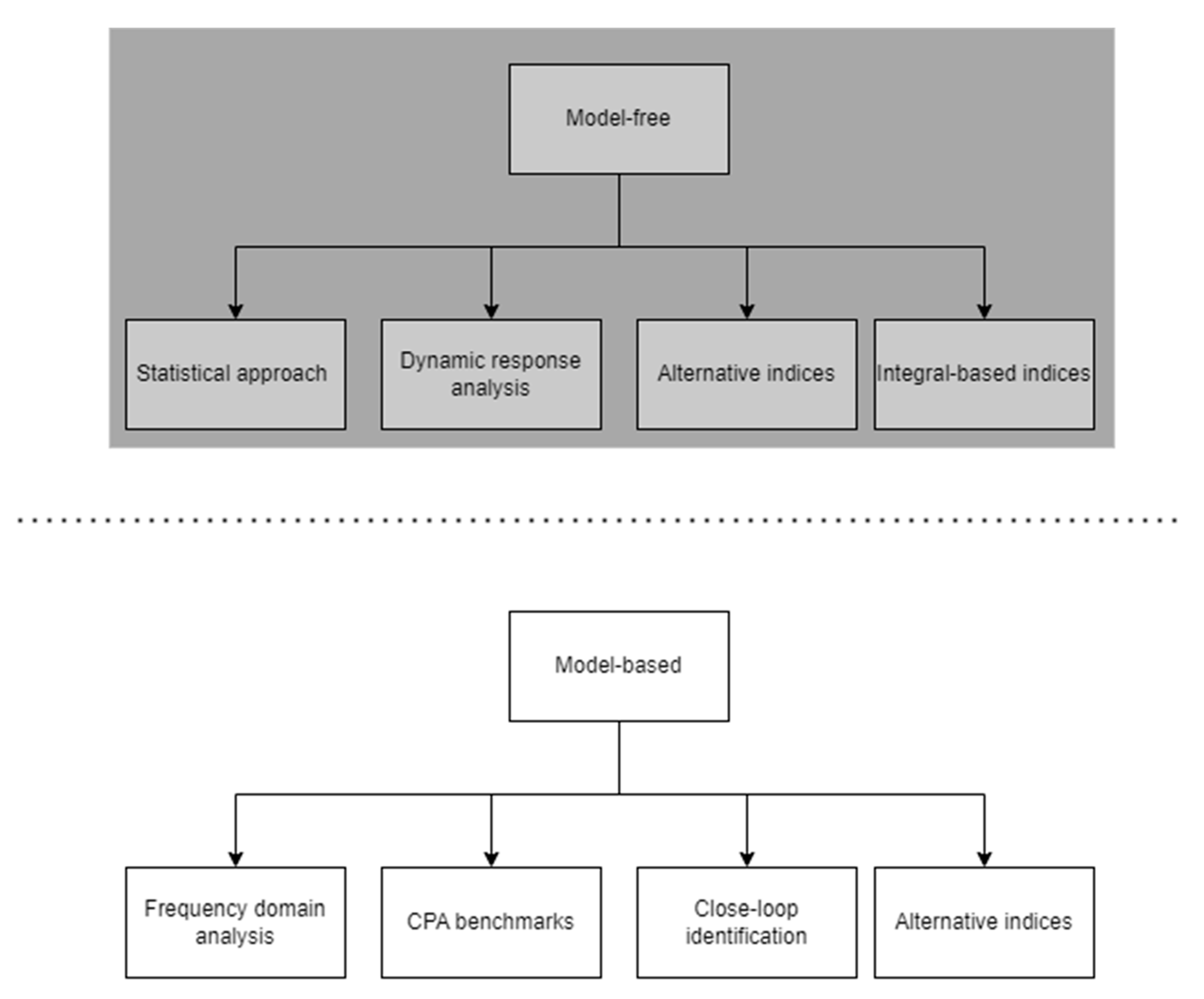
2.1. Implemented CPM Indices

CPM methods for demonstration were chosen based on the criteria previously mentioned. The methods should perform without the need for modeling of the process. A priori knowledge of the process should not be needed for estimating the control performance. As such, the methods described in the following section were chosen.

Integrated Squared Error (ISE, Equation (1)) is calculated as a function of time and in a sliding window. Here, a sliding window of one day is selected as:

$$ISE={{\displaystyle \int }}_{n-x}^{n}e{\left(t\right)}^{2}dt,$$

(1)

where ISE is comprised of the sum of squared errors (e(t)) between the current time (n) and the duration of the sliding window (x).

For the performed step changes, the Integral of Time-weighted Absolute Error (ITAE, Equation (2)) is monitored for identifying longer period faults in the process. The longer a fault is present, the larger the time weight grows and directly increases the metric. The time weight used is the time since the last setpoint change:

$$ITAE={{\displaystyle \int }}_1^{w}t\left|e\left(t\right)\right|dt,$$

(2)

where ITAE is the sum of the absolute values of errors (e(t)) multiplied by the time since the last setpoint change (w). Additionally, Amplitude Index (AMP, Equation (3)) is used to measure the ratio between the maximum amplitude of process error and the size of the performed step change. The value is obtained from the minimum and maximum values after the rise time period, as in [3]:

$$AMP=\frac{y_{max}-y_{min}}{\mathsf{\Delta }{y}_{sp}},$$

(3)

where $y_{max}$ and $y_{min}$ are the maximum and minimum values, respectively, of the process value after the rise time and $\mathsf{\Delta }{y}_{sp}$ is the magnitude of the performed step change.

The difference from normal operation in the process can be identified by utilizing the measurement error residuals and comparing the distribution to a selected time period from normal operation. Kullback–Leibler divergence (KL, Equation (4)) [19] provides a measurement for difference between the two datasets. In real processes, obtaining data from the normal operation may prove difficult, especially if the process has been in operation for a while and unknown disturbances may have occurred. Kullback–Leibler divergence has been previously adapted to an index in MIMO controller performance monitoring [20]:

$$KL={{\displaystyle \int }}^{ }{h}_1\log \frac{h_1}{h_2}dx,$$

(4)

where $h_1$ is the reference dataset and $h_2$ is the dataset in the chosen sliding window. Additionally, histogram intersection (HI, Equation (5)) [21] and Euclidean distance (ED, Equation (6)) [22] are used here to estimate the difference between the reference data and the sliding window testing datasets:

$$HI=\frac{{{\displaystyle \sum }}_{j=1}^{m}min\left(h_{1,m},h_{2,m}\right)}{{{\displaystyle \sum }}_{j=1}^m{h}_{2,m}},$$

(5)

$$ED=\sqrt{{\displaystyle \sum }_{j=1}^m{\left(h_{1,m}-h_{2,m}\right)}^2},$$

(6)

where the datasets $h_1$ and $h_2$ are divided into m histogram bins.

In addition, a commercial CPM tool was applied to the studied process. Overall Controller Efficiency (OCE) is a method developed by Insta Advance. The idea of OCE was inspired from a more general framework called OEE and is an adaptation of it in the context of PID controller performance. OCE defines one number that describes one PID controller’s history, present, and future ability to function in a specified task. The main point in OCE is to follow the trend of the OCE value, and a continuous decrease in the OCE value may indicate the need for action. On the contrary, an increase in the OCE value can show the recovery or improvement of PID controller efficiency. OCE was first developed for detecting long-term phenomena (e.g., crawling due to wearing), but in this paper, OCE’s suitability to detect short-term phenomena has been examined in detail in the experimental part.

In general, OCE_total is a product of three separate factors, as indicated in Equation (7):

$$OC{E}_{total}=OC{E}_a\times OC{E}_p\times OC{E}_q.$$

(7)

In Equation (7), OCE_a is the availability, or the portion of time the controller autonomously produces good-quality data. OCE_p is the performance, or the accuracy to follow the setpoint value without oscillation, and OCE_q is the quality, or the ability to continue as part of the production process in the future.

In this application, availability is calculated based on the proportion of automatic and manual control of the studied control loop, while performance is related to the setpoint tracking error. Quality is related to several indices describing the control loop performance in long-term trends. The details of the quality factors are omitted due to company confidentiality reasons. Overall, the calculation of the OCE_total value relies on a statistical algorithm. The OCE method includes parameters to finetune the process, and in this paper, the two parameters that describe the number of days in the buffer and evaluation are considered. In both cases, a value of 10 was used.

Since OCE_total represents a product of the three aforementioned factors, it is sensitive to variability in any of the indices. An extreme example is that if any of the factors are zero, the whole OCE_total value becomes zero. Moreover, in the case of asymmetric indices, OCE may become less appropriate.

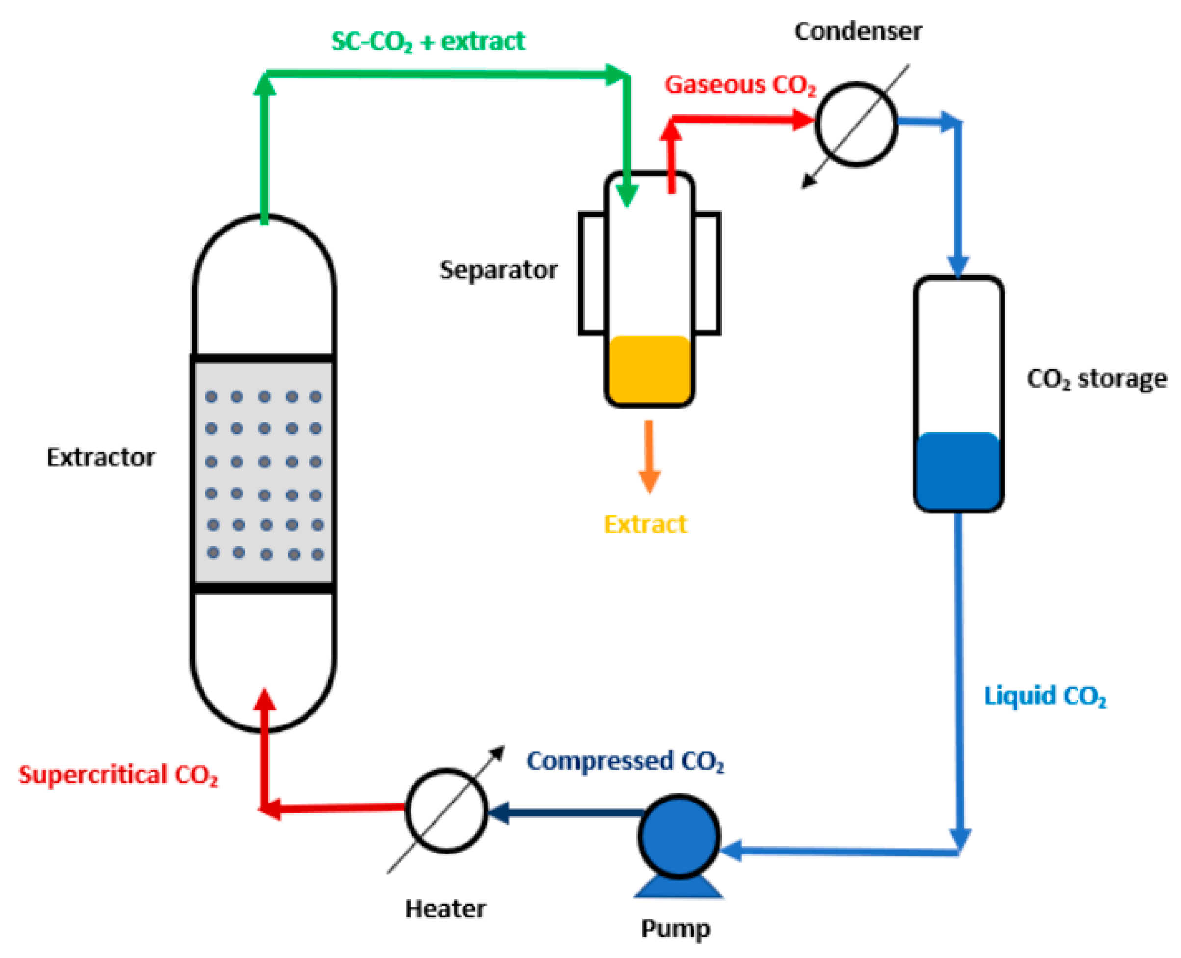
2.2. Simulated Process

A supercritical fluid extraction (SFE) process utilizes properties of a supercritical fluid to extract product from a raw material. Carbon dioxide (CO₂) is commonly used as the supercritical fluid due to the properties of CO₂, with it being sufficiently easy to achieve pressure (73.8 bar) and temperature (32.1 °C) for the critical point. The process consists of six parts, namely, the extraction reactor, extract separator, condenser, CO₂ storage, CO₂ flow pre-heater, and pump, as shown in Figure 2. A set of central composite design experimental test runs were performed and state-space models for the process components were identified in [23,24]. Thus, the simulator used represents a validated model of the physical process.

One control loop from the previously identified simulator was isolated for this work. The selected discrete-time, state-space model (see Equations (8) and (9)), namely, the CO₂ flow, was identified from open-loop measurements of the original work [17,18], while other portions of the simulator were identified with the existing PID control in the process. The CO₂ flow is the controlled variable, y(n), and valve position is the manipulated variable, u(n). The second input is the external variable, ΔP. In this study, the external variable is utilized as a disturbance, with a value of 0 in normal operation.

$$\begin{gathered} x\left(n+1\right)=\left[\begin{array}{cc}0.9895& 0.03677\\ -0.01237& 0.9649\end{array}\right]x\left(n\right)+ \\ \left[\begin{array}{cc}-2.520e-05& -1.673e-06\\ -2.199e-04& -5.346e-06\end{array}\right]u\left(n\right), \end{gathered}$$

(8)

$$y\left(n\right)=\left[\begin{array}{c}-10.22\\ -0.1235\end{array}\right]x\left(n\right)\left(+\left[\begin{array}{c}0\\ 0\end{array}\right]u\left(n\right)\right),$$

(9)

The state-space model for the supercritical fluid extraction process was implemented to MATLAB^® and Simulink^® software (Version R2020b Update 2). PI control, with parameters 8 for proportional gain and 0.2 for integral gain, was added to the simulator, and the parameters were kept constant for the simulations. As the simulator models the CO₂ flow into the reactor, the lower limit for the output was limited to 0. The closed-loop process settling time after a step change is approximately 400 s. Therefore, the simulation scenario involved setpoint changes every 1200 s. The setpoint values were selected randomly from an even distribution between 0 and 0.8, with an interval of 0.1. With these chosen step changes, a representative dataset for the process was obtained for the whole area of operation of the process. Additionally, having frequent step changes in the process, the overall size of the dataset could be reduced, decreasing computing time in the later stages of the demonstration. The obtained measurement data were then sampled every 10 s to further reduce the size of the data matrix.

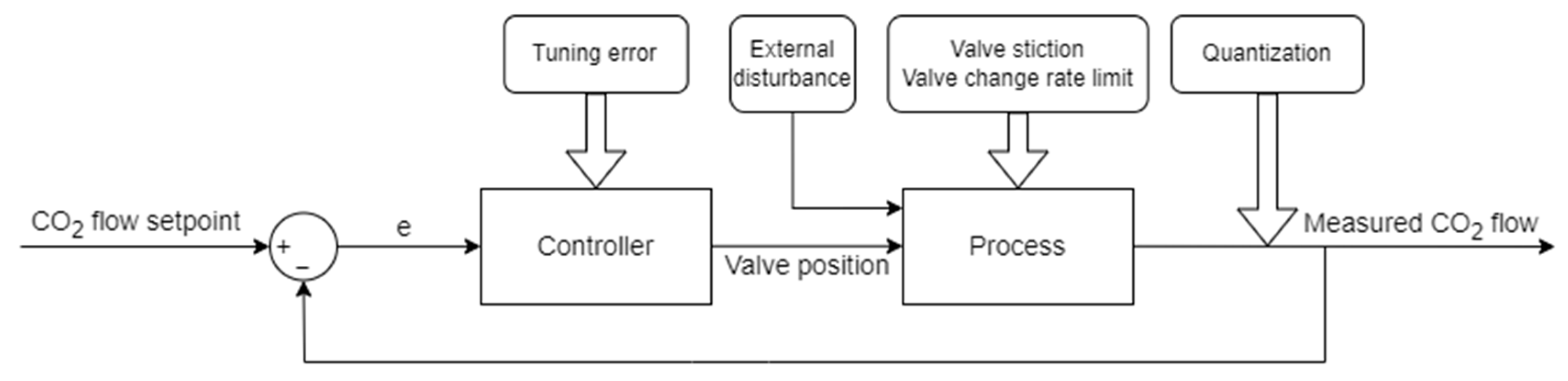
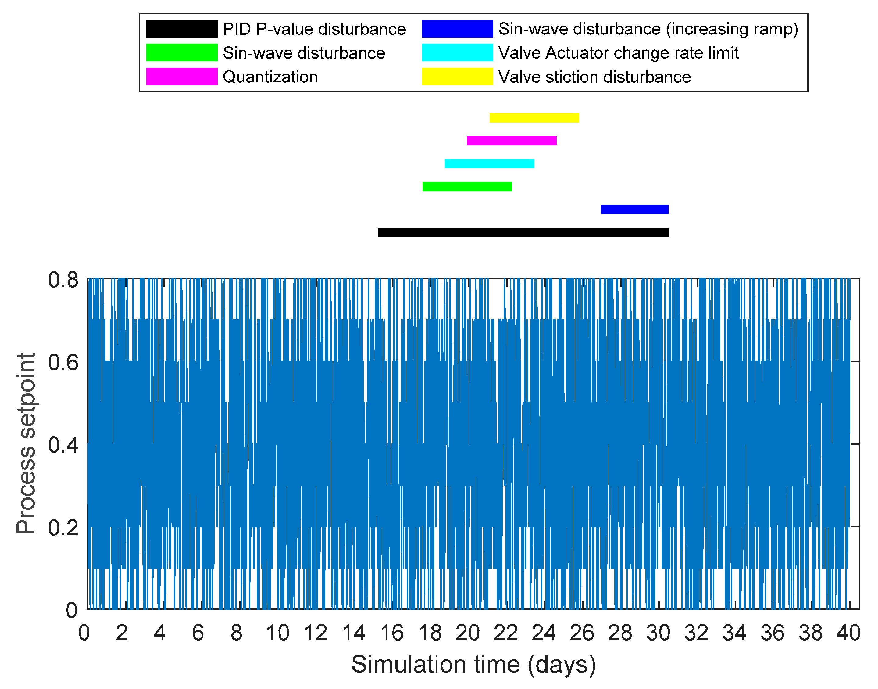
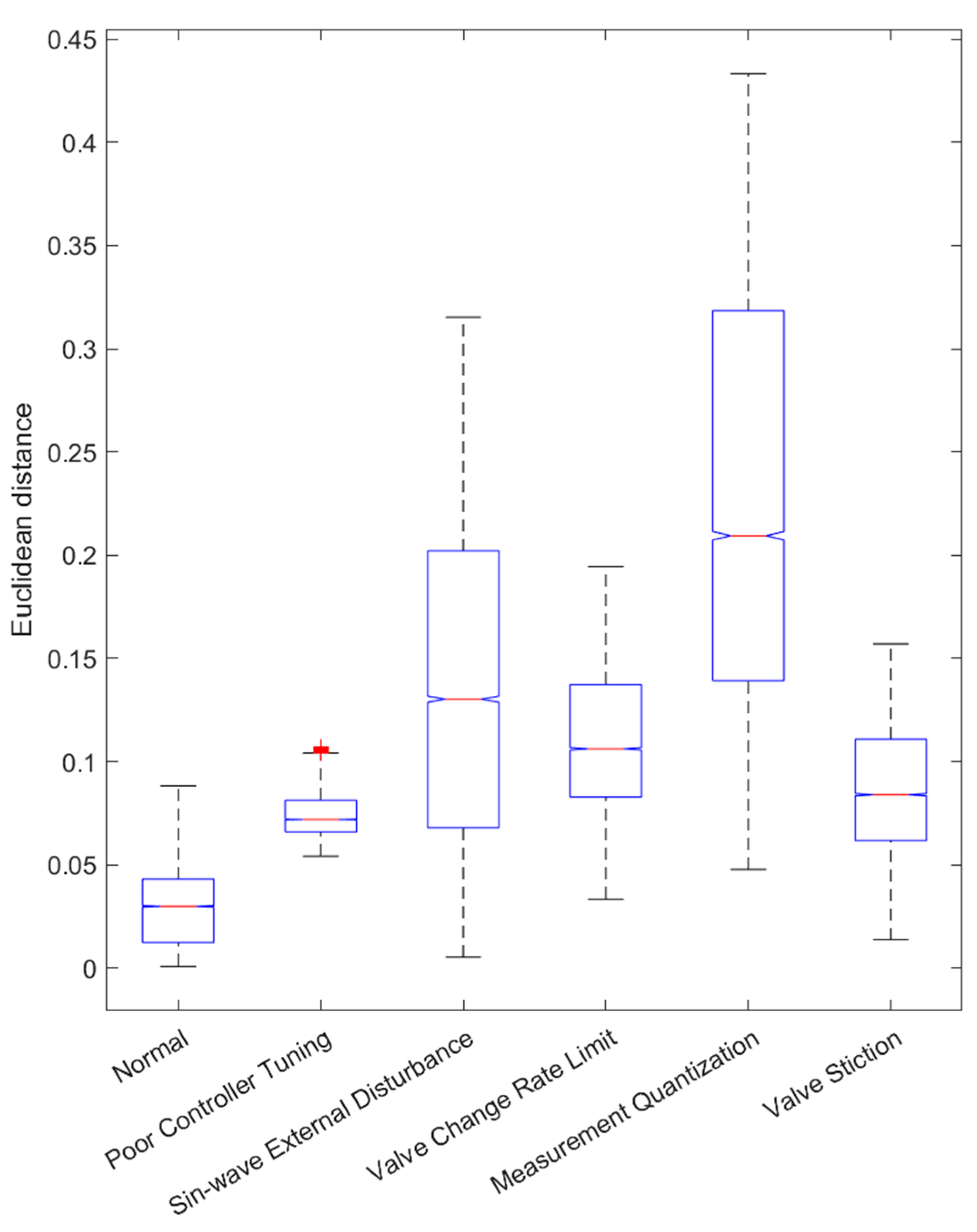
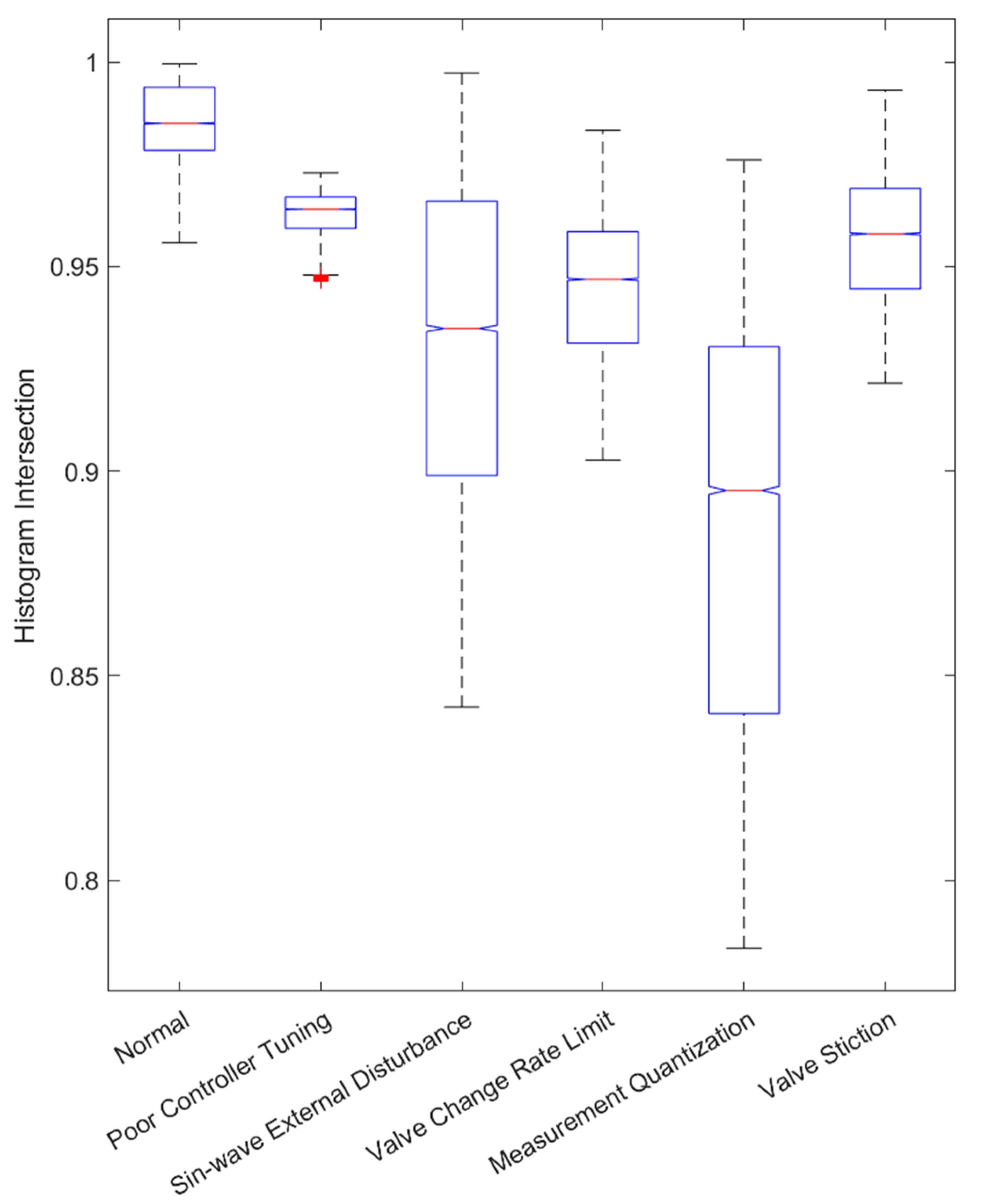
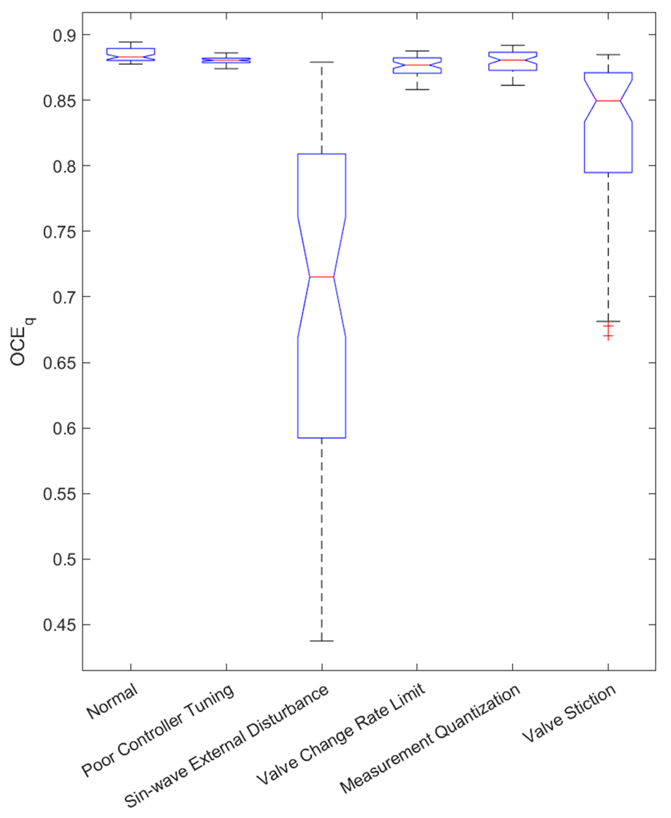
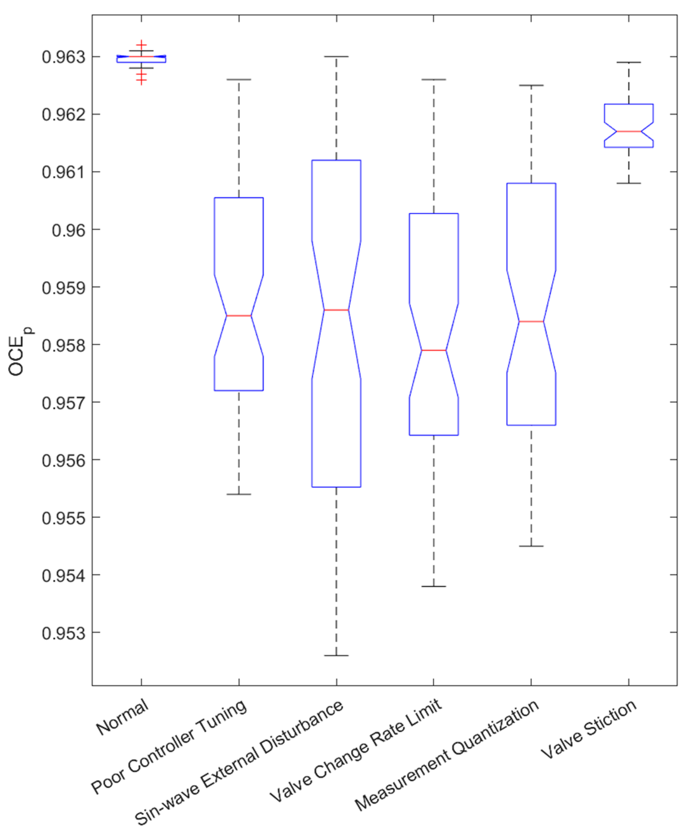
2.3. Simulated Faults

In Case 1, the performance of the CPM methods for different kinds of faults was studied in a long simulation period. The faults were added to the simulated process, first occurring individually and later simultaneously. From the common faults presented in [5], the following faults were used in this work:

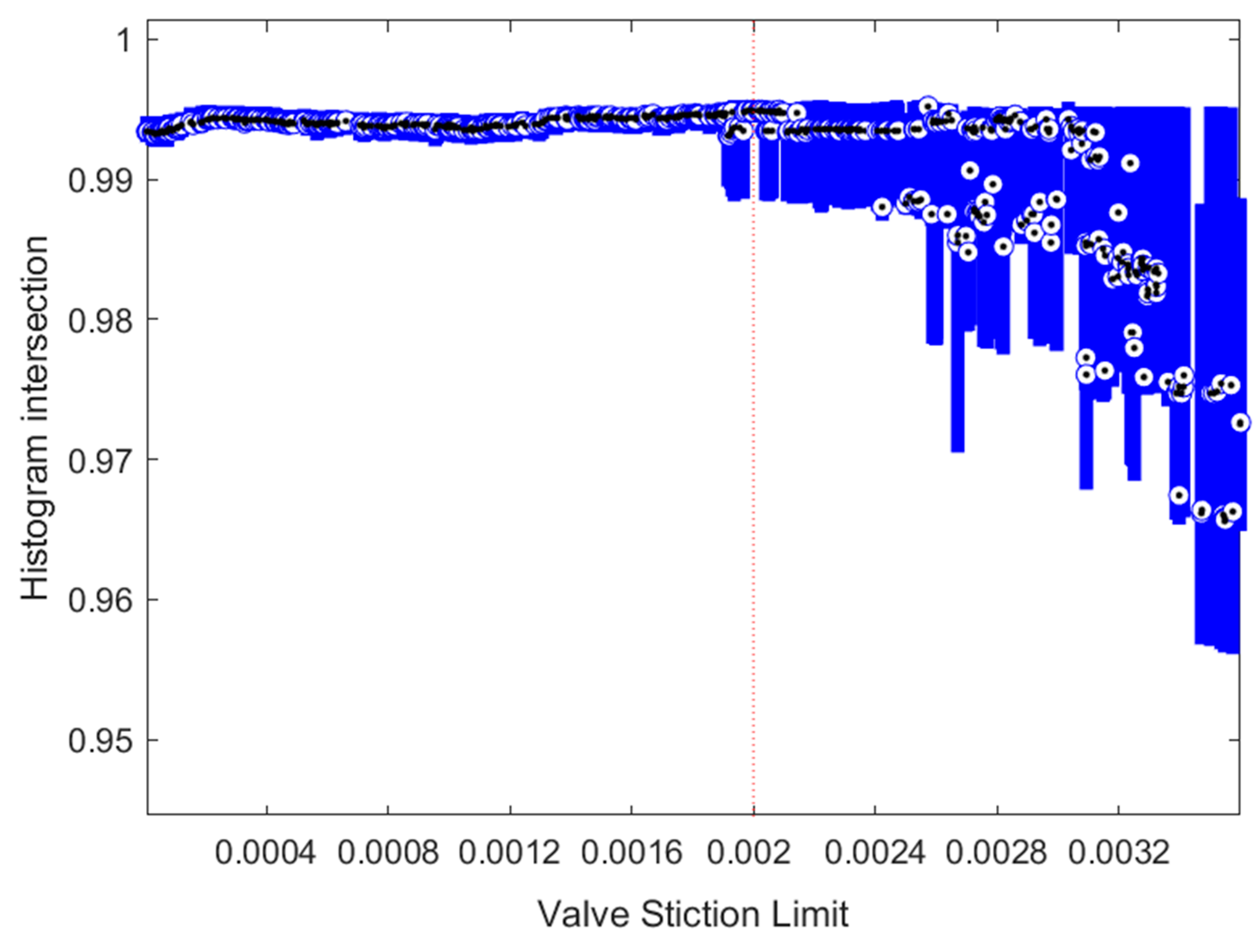
• Valve stiction, where a certain difference between the previous and new controller output is required in order to have an effect on the actuator position. Nominally, the valve stiction in a faulty situation was set to 0.002.
• Valve change rate limit—simulating a scenario where the motor controlling the valve has a sudden fault limiting the speed of the valve change. In this case, the speed is limited to 0.04 valve rotations/s.
• Sin-wave with a constant amplitude of 75 bar, a frequency of 0.00002 Hz, and a rising amplitude (from 0 to 141.6 bar), with a frequency of 0.0001 Hz representing an external disturbance to the process. This disturbance acts as the second input variable in the state-space model (pressure error), as described in Section 2.2.
• Quantization, where the measured process value fed back for the controller is quantized within an accuracy of 0.08 L/min instead of a floating number. This value was selected to produce a noticeable effect on the process control behavior.
• PID controller tuning error, where the value of the P-parameter is changed from 8 to 0.8 for the duration of the fault.

The simulator with the implemented control and faults is displayed in Figure 3.

The faults are enabled one by one as follows. The first 15 days of the simulation are fault-free. The following 2.3 days of the simulation have only one fault activated. The remaining faults are then enabled one by one, every 1.2 days, until each fault is enabled. The faults are then disabled one by one every 1.2 days, following the order of activation for the faults. Thus, during the period from 20.8 to 22.0 days, all faults are present. Afterwards, a rising sin-wave external fault is enabled during the time period of 26.6 to 30.1 days. The final 9.9 days of the simulation are without faults, where restoration to the normal state can be observed.

Figure 4 depicts the simulation of 40 days containing the setpoint changes mentioned in Section 2.3 and the faults described above for the case with PID p-value disturbance. Simulations were repeated with different fault scenarios for a comparison of different measurement metrics with each fault case.

In Case 2, the robustness of the methods was tested. A simulation dataset with different values for fault intensities was obtained, focusing on the valve stiction fault. First, a simulation with no faults was performed to obtain a reference dataset. A total of 500 different simulations were performed with different fault intensities for valve stiction, chosen randomly for each simulation from an even distribution. For the valve stiction intensity, a required difference from 0 to 0.0036 between new and old actuator values was chosen. To speed up the simulation, 800 s between setpoint changes was used instead of the 1200 s used in Case 1. With the reduction of the simulation time, the OCE method does not perform adequately and is left out for this case.

3. Results

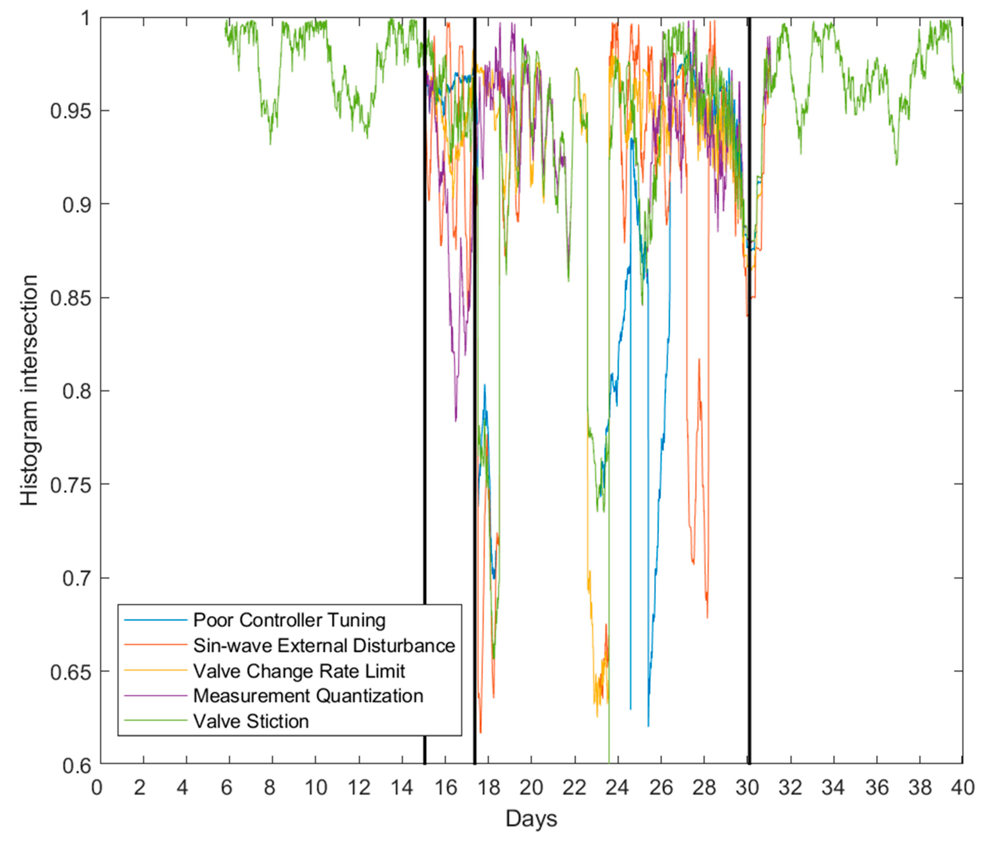
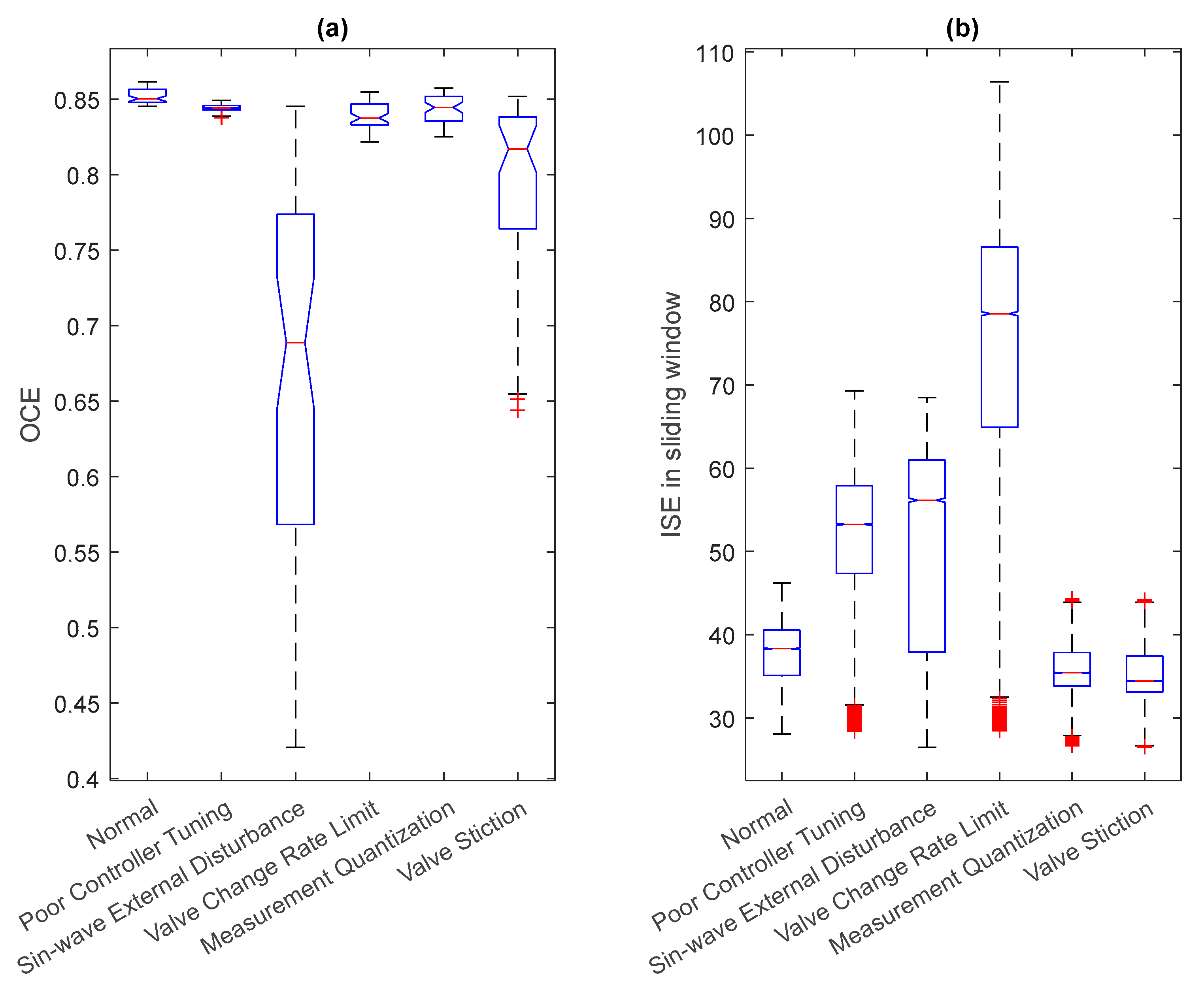
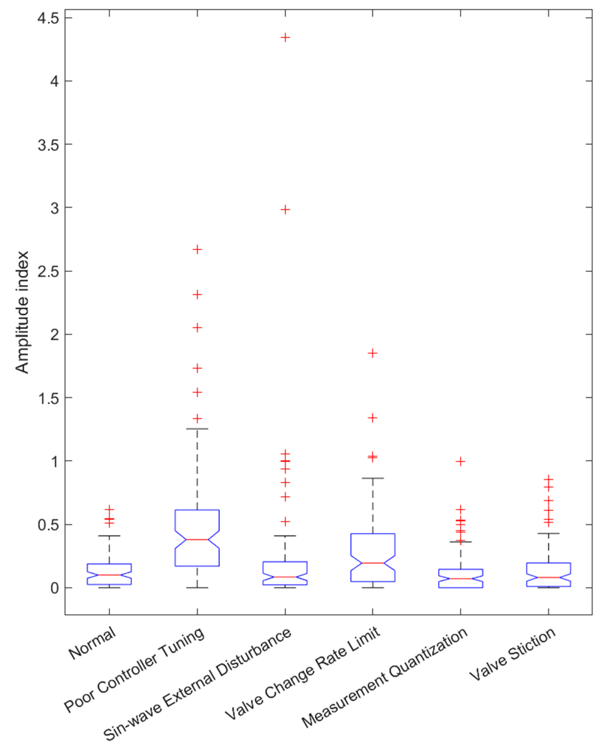
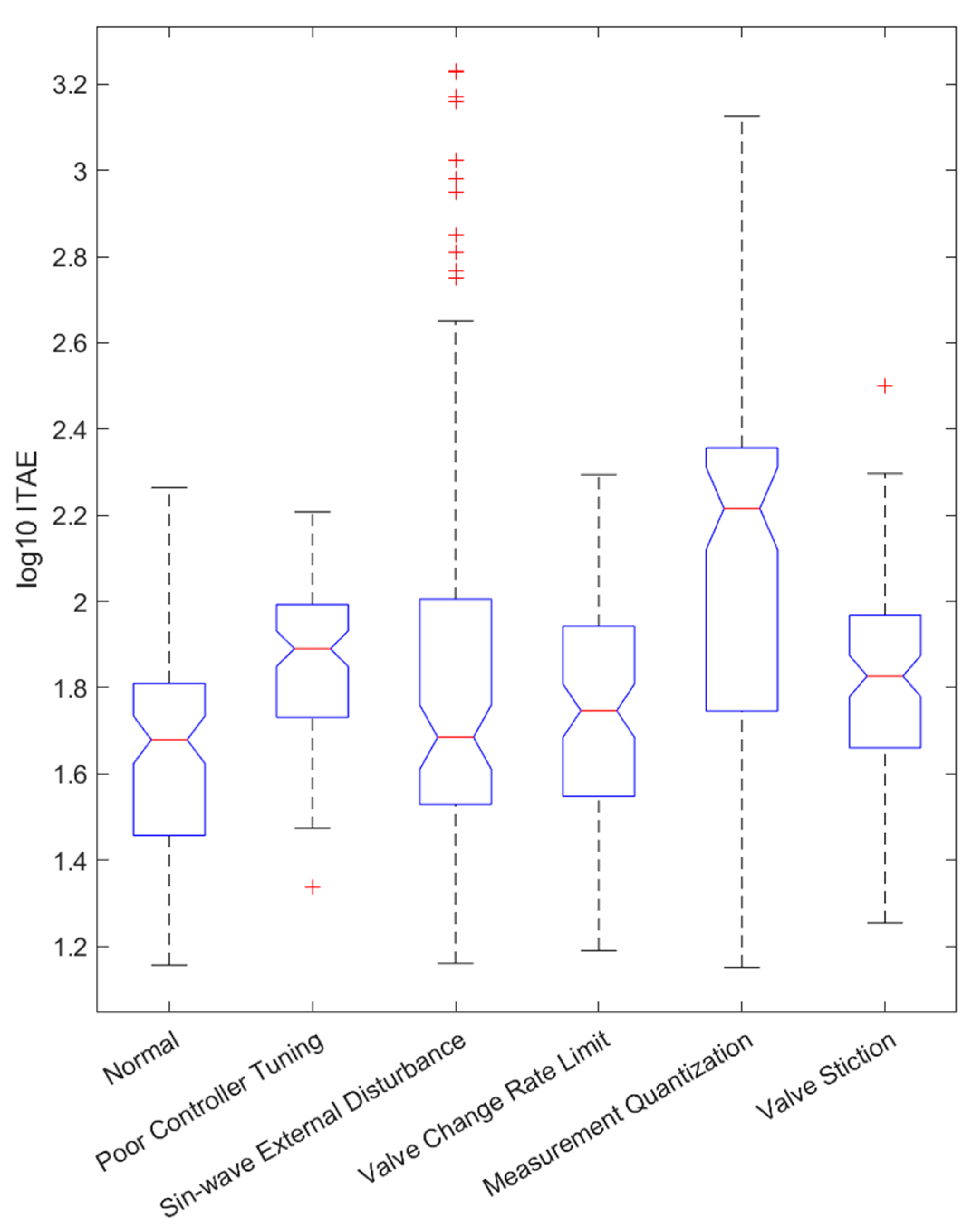
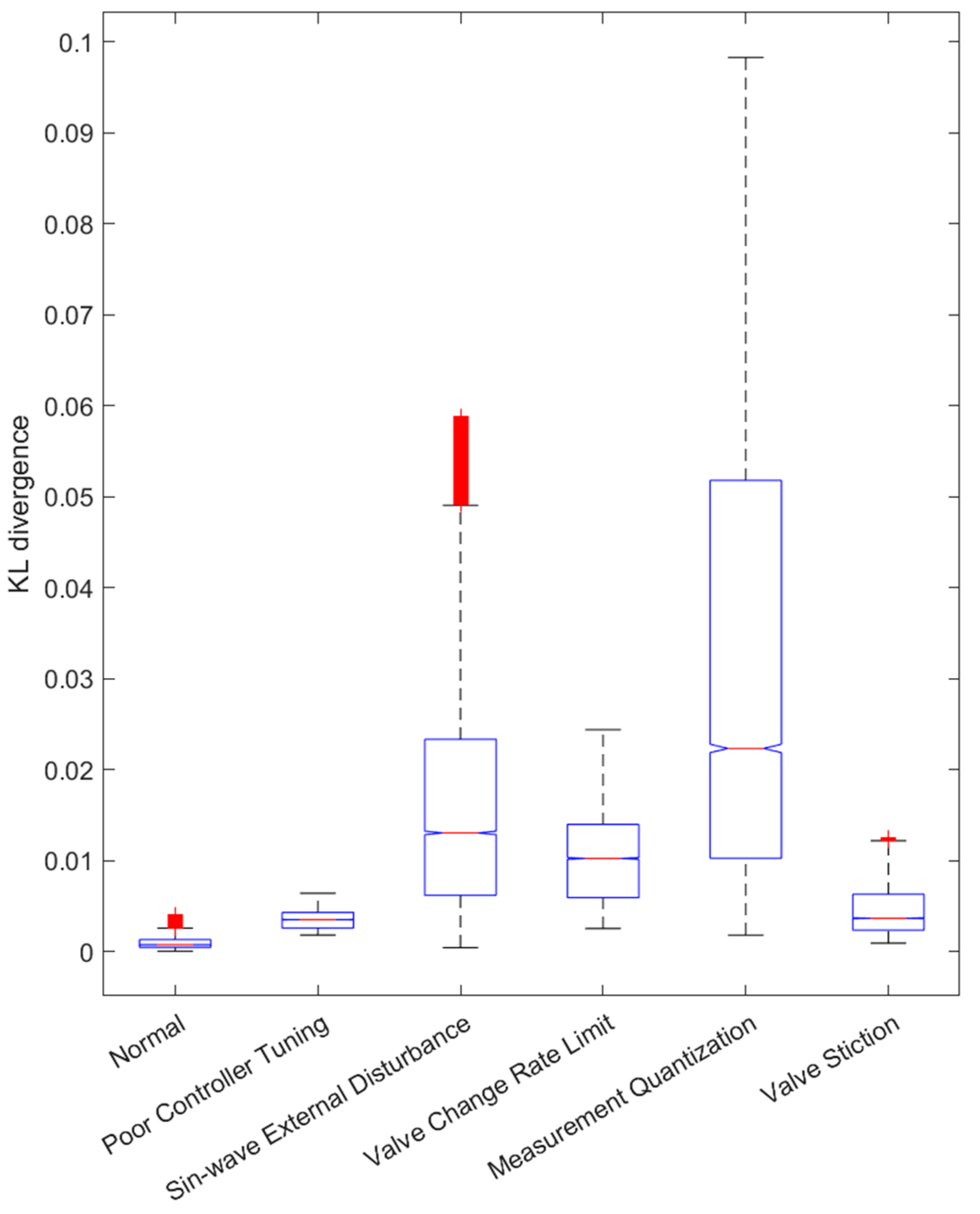
3.1. Case 1. Identification of Faults with Different CPM Methods

Kullback–Leibler divergence, histogram intersection, and Euclidean distance are used in this case to compare the selected reference dataset to a testing set selected from a sliding window of one day (8640 data points). The training data are selected from the beginning of the simulation with a size of 50,000 data points. The start of the dataset is known to represent the normal behavior of the process and can thus provide an accurate reference for the methods. Additionally, the number of bins for the histograms used is set to 8.

In practice, identifying normal behavior of the process is a challenge for accurate monitoring in industrial processes. For this purpose, the utilized simulator allows for a fault-free scenario when identifying the normal process behavior and provides means for estimating the performance of the chosen CPM indices.

In Figure 5, the differences between the reference data (first 50,000 data points) and a testing set selected with a sliding window of size 8640 (1 day) can be seen for the histogram intersection method. For the HI method, the high index values indicate good performance as the statistical properties of the test set are close to the reference data obtained during a normal control loop performance. Slight changes in the metrics occur even in normal operation (days 6–15), due to the randomly chosen setpoints. During the periods with faults, the index clearly deviates from the values in normal operation. After the simulated faults have ceased, the index returns to nominal value range, indicating a good performance of the CPM method. Similar performance was observed for the Kullback–Leibler divergence and Euclidean distance metrics.

However, with these methods, properties of the training data can affect the resulting metrics. Deviations from the training data have a significant effect and retraining may be necessary to adapt to an evolving process environment. Moreover, selection of the size of the sliding window for the metrics affects the resolution of the results. With a larger window size, the observation of a fault might be delayed as a lower proportion of the window is from faulty data. Determining alarm limits is dependent on the process as tolerances can vary.

Identification of an individual fault was considered by comparing a period of the simulation where one fault was present with an equal-sized duration from the fault-free period. In Figure 6a, this comparison for the OCE method was performed and presented as a boxplot for normal, fault-free data, and separately for the five fault scenarios. A high OCE_total value corresponds to good control, whereas lower values indicate decreased control loop performance. It can be seen that the OCE method can separate all of the faulty situations from the normal operation, as the notches of the plot (95% confidence) do not overlap. The process was repeated for all metrics (boxplots presented in Appendix A, Figure A1, Figure A2, Figure A3, Figure A4, Figure A5, Figure A6 and Figure A7) and qualitatively compiled in

Table 1. Qualitative performance of CPM indices. The fault situations marked with X showed statistically significant difference in the monitored index between normal and faulty operation.

CPM Index	Cont. Tuning	Ext. Dist.	Rate Limit	Quant.	Valve Stiction
ISE	X	X	X	-	-
ITAE	X	-	-	X	X
AMP	X	-	X	-	-
KL	X	X	X	X	X
ED	X	X	X	X	X
HI	X	X	X	X	X
OCEp	X	X	X	X	X
OCEq	-	X	X	-	X
OCEtotal	X	X	X	X	X

. The fault was considered to be identified when the index significantly differed from the normal behavior in the expected direction. As indicated in Figure 6b, ISE shows a lower index value for the fault scenarios’ quantization and valve stiction, although it is expected that the integrated error value would increase in the presence of fault. According to Table 1, among the tested CPM methods, KL, HI, ED, OCE_p, and OCE_total could detect the decreased control loop performance simulated in Case 1.

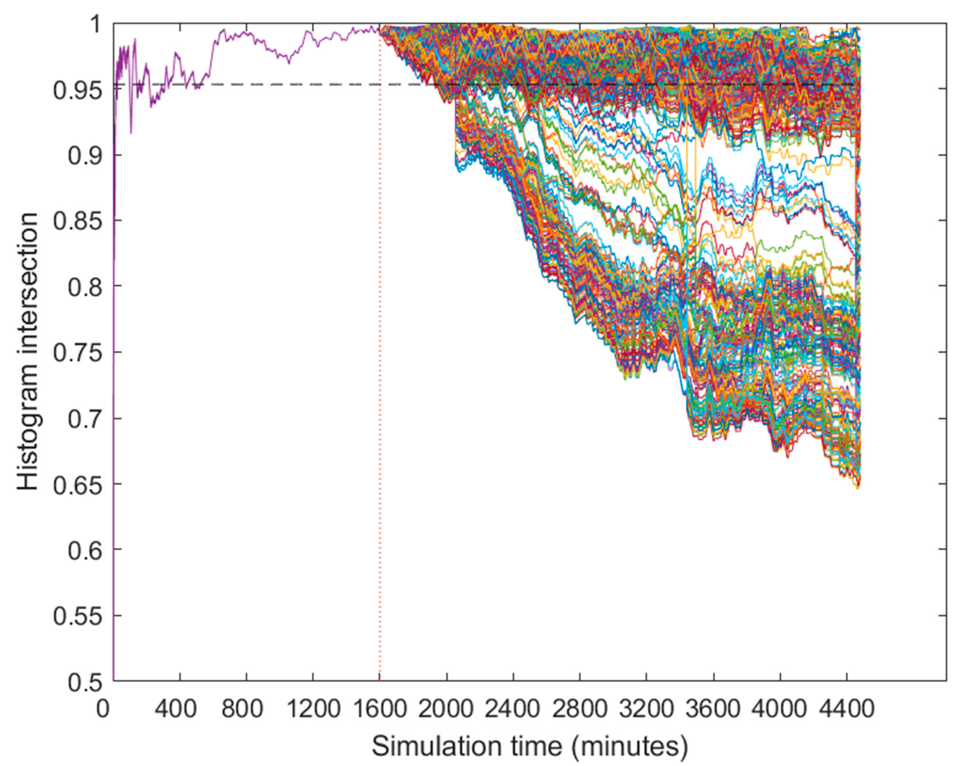
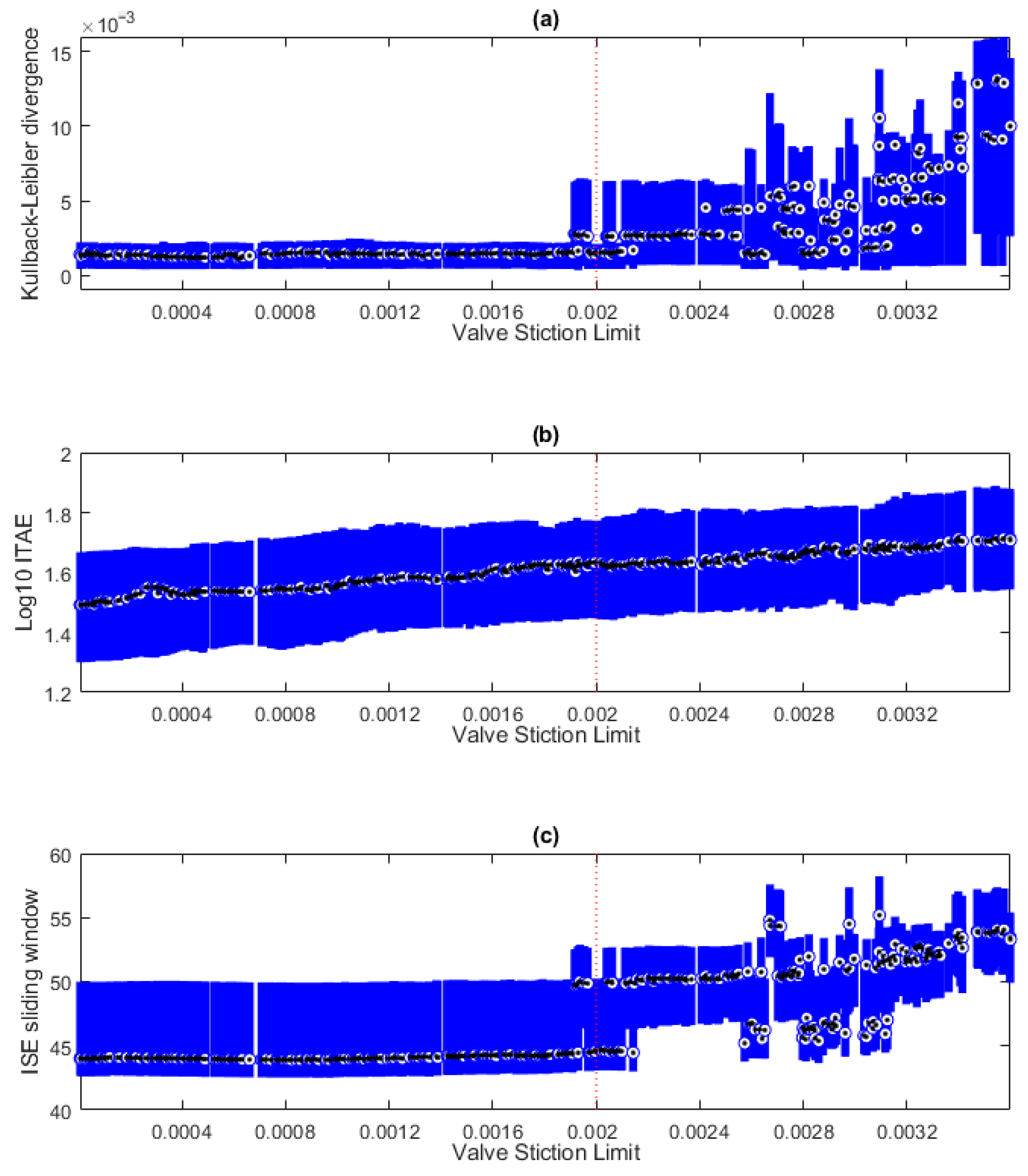
3.2. Case 2. Robustness of the Methods with Varying Fault Intensities

The robustness of the demonstrated methods was considered with the second simulation case, where the fault intensity for valve stiction was changed randomly for 500 different simulations. The resulting index values for the histogram intersection are shown in Figure 7.

It can be seen in Figure 7 that some of the intensities for valve stiction can be identified, as the index value clearly decreases below the normal operation (dashed horizontal line). However, most of the index values are near normal operation limits, suggesting a limited performance of the CPM index in this case. To improve the identification of the fault, the CPM method parameters need to be adjusted. After testing a different number of bins for the histogram intersection method, the best results in terms of the method’s robustness to different fault intensities was achieved with a parameter value of 15 bins. Figure 8 depicts the result. It is notable that the resolution (absolute values of the index) of the method was now considerably lower in comparison to the results in Figure 7.

Valve stiction was identified for different methods with varying degrees of intensity for the fault required. In Figure 8 and Figure 9, the metrics are drawn as a boxplot (median, and lower and upper quartiles) as a function of the fault intensity. HI (Figure 8), ED, and KL (Figure 9a) can identify the fault well, as the intensity of the fault increases above 0.002. AMP performed poorly with all chosen intensities, due to the nature of the valve stiction fault. Among the studied CPM methods, ITAE showed the most robust behavior for different intensities of the valve stiction, shifting from the normal operation with even small disturbance values, as shown in Figure 9b. ISE also performed well, as shown in Figure 9c.

The sensitivity of the demonstrated indices was compiled in

Table 2. Index performance with different fault intensities.

CPM Index	Lowest Identified Fault Intensity	Highest Non-Identified Fault Intensity	Identified Fault Intensities	Identification Percentage
ISE	1.4 × 10−3	0.0015	307/500	61.4%
AMP	-	-	0/500	0%
ITAE	1.1 × 10−3	0.0014	345/500	69%
KL	6.9 × 10−6	0.0026	447/500	89.4%
HI	2.5 × 10−5	0.0031	194/500	38.8%
ED	2.5 × 10−5	0.0031	194/500	38.8%

, where statistically significant difference (95% confidence) for the medians in the fault-free simulation and the simulations with different fault intensities were compared.

The results suggest that KL, HI, and ED can identify small fault intensities with some accuracy, but only reach accurate identification with the highest intensities. Additionally, the absolute values of these metrics were low, and the performance may vary in more non-ideal conditions. AMP could not identify any of the implemented fault intensities. Integrating methods ISE and ITAE performed well and had only a small range between the lowest identified and highest non-identified fault intensities.

4. Discussion

The current state of control performance monitoring methods was explored, and different model-free CPM methods were chosen for a demonstration case with the aim of providing easily adaptable methodologies for control loop performance monitoring in industrial applications. Some of these methods are widely used in control loop design and tuning, and this work further adapts these methods in a dynamic control performance monitoring application. A simulated environment was used to obtain a representative dataset for testing, with the possibility of including different faults in different time periods in the simulation.

Among the studied methods, histogram intersection well identified the control error residual difference from the reference data. Increased error from poor control results in an abnormal distribution. However, the metric is heavily dependent on the conditions from which reference data were obtained. Naturally causing drift and other changes in the process can cause the metric to shift from an optimal area, even though the process may perform adequately. As such, multiple metrics should be monitored for verifying the results of other metrics and observing the actual state of the process. One option to facilitate this is to take the approach used in the OCE method, which uses a product of several indices to assess the overall controller performance. For example, the histogram intersection is naturally scaled to values between 0 and 1, thus being an appropriate candidate for such a combined CPM index.

With respect to the second case with varying fault intensities, the KL, HI, and ED methods performed rather poorly. The metrics mostly stayed at levels of normal operation with the original method parameters. Adjusting the parameters for these methods allowed accurate identification of the fault with the valve stiction values above 0.0031, as seen in Table 2. However, robustness was compromised, with the methods only falling slightly below the normal operation levels (for example, the median stayed above 0.96 for histogram intersection in the highest valve stiction cases). The metrics could identify some of the lowest fault intensities with decent accuracy but missed the identification of some of the highest intensities. Amplitude Index performed poorly in the second case; however, the metric has utilization potential in different fault cases. The integral methods ITAE and ISE performed well, with ISE identifying 61.4% and ITAE 69% of the varying fault intensities. This can be explained by the nature of the implemented fault, which caused residual setpoint error that integrating methods can identify well. Additionally, due to the nature of the simulation, the chosen sliding window has a large and very homogenous number of step changes. In practice, setpoint changes can happen infrequently and at random time intervals. As such, applicability of the methods should be considered when implementing CPM tools.

This paper focused on a single control loop case to build on a solid foundation for further research. Multiple-input multiple-output control could prove an interesting topic in the future. The setpoint changes utilized in the demonstrations were chosen to be rather short, while industrial applications may run in the same state for weeks at a time. Additionally, only one process was utilized for the simulations. Differences in process dynamics may cause differences in the behavior of the control performance monitoring metrics. Thus, the performance of the methods should also be studied for different types of data to ensure industrial applicability. Further, the demonstration presented was based on simulated, noise-free data. Stability and tuning of the methods will require more attention with real data, where noise is present or partially filtered.

5. Conclusions

In this work, it was found that the Kullback–Leibler divergence, Euclidean distance, histogram intersection, and OCE method could identify all the simulated fault scenarios in the first simulation case. In the second case, the robustness and sensitivity of the metrics were further analyzed in the presence of valve stiction fault, where the integral-based ISE and ITAE metrics demonstrated robust performance.

Control performance may suffer due to different sources of faults and different CPM methods’ performance varies depending on the nature of the fault. Thus, a combination of methods should be considered as a monitoring solution. As noted in this work, the OCE method consisted of several factors and responded well to different fault scenarios.

References

1. Domański, P.D. Performance Assessment of Predictive Control—A Survey. Algorithms 2020, 13, 97. [Google Scholar] [CrossRef] [Green Version]
2. Al Soraihi, H.G. Control Loop Performance Monitoring in an Industrial Setting. Master’s Thesis, RMIT University, Melbourne, VIC, Australia, 2006. [Google Scholar]
3. Jamsa-Jounela, S.-L.; Poikonen, R.; Georgiev, Z.; Zuehlke, U.; Halmevaara, K. Evaluation of control performance: Methods and applications. In Proceedings of the International Conference on Control Applications, Glasgow, UK, 18–20 September 2002; Volume 2, pp. 681–686. [Google Scholar] [CrossRef]
4. Starr, K.D.; Petersen, H.; Bauer, M. Control loop performance monitoring—ABB’s experience over two decades. IFAC-PapersOnLine 2016, 49, 526–532. [Google Scholar] [CrossRef]
5. Bauer, M.; Horch, A.; Xie, L.; Jelali, M.; Thornhill, N. The current state of control loop performance monitoring—A survey of application in industry. J. Process Control 2016, 38, 1–10. [Google Scholar] [CrossRef]
6. Holstein, F. Control Loop Performance Monitor. Lund Institute of Technology. 2004. Available online: https://lup.lub.lu.se/luur/download?func=downloadFile&recordOId=8848037&fileOId=8859439 (accessed on 16 June 2022).
7. Múnera, J.G.; Jiménez-Cabas, J.; Díaz-Charris, L. User Interface-Based in Machine Learning as Tool in the Analysis of Control Loops Performance and Robustness. In Computer Information Systems and Industrial Management; Saeed, K., Dvorský, J., Eds.; In Lecture Notes in Computer Science; Springer International Publishing: Cham, Switzerland, 2022; pp. 214–230. [Google Scholar] [CrossRef]
8. Grelewicz, P.; Khuat, T.T.; Czeczot, J.; Nowak, P.; Klopot, T.; Gabrys, B. Application of Machine Learning to Performance Assessment for a Class of PID-Based Control Systems. IEEE Trans. Syst. Man Cybern. Syst. 2023, 2023, 1–13. [Google Scholar] [CrossRef]
9. Stamatis, D.H. The OEE Primer: Understanding Overall Equipment Effectiveness, Reliability, and Maintainability; Productivity Press: New York, NY, USA, 2011. [Google Scholar] [CrossRef]
10. Vorne Industries, Inc. What Is OEE (Overall Equipment Effectiveness)?|OEE. 2022. Available online: https://www.oee.com/ (accessed on 4 November 2022).
11. Ghaleb, M.; Taghipour, S. Assessing the impact of maintenance practices on asset’s sustainability. Reliab. Eng. Syst. Saf. 2022, 228, 108810. [Google Scholar] [CrossRef]
12. Choudhury, M.A.A.S.; Shah, S.L.; Thornhill, N.F. Diagnosis of poor control-loop performance using higher-order statistics. Automatica 2004, 40, 1719–1728. [Google Scholar] [CrossRef] [Green Version]
13. Horch, A. A simple method for detection of stiction in control valves. Control Eng. Pract. 1999, 7, 1221–1231. [Google Scholar] [CrossRef]
14. Howard, R.; Cooper, D. A novel pattern-based approach for diagnostic controller performance monitoring. Control Eng. Pract. 2010, 18, 279–288. [Google Scholar] [CrossRef]
15. Mok, R.; Ahmad, M.A. Fast and optimal tuning of fractional order PID controller for AVR system based on memorizable-smoothed functional algorithm. Eng. Sci. Technol. Int. J. 2022, 35, 101264. [Google Scholar] [CrossRef]
16. Ekinci, S.; Hekimoğlu, B. Improved Kidney-Inspired Algorithm Approach for Tuning of PID Controller in AVR System. IEEE Access 2019, 7, 39935–39947. [Google Scholar] [CrossRef]
17. Ziane, M.A.; Pera, M.C.; Join, C.; Benne, M.; Chabriat, J.P.; Steiner, N.Y.; Damour, C. On-line implementation of model free controller for oxygen stoichiometry and pressure difference control of polymer electrolyte fuel cell. Int. J. Hydrogen Energy 2022, 47, 38311–38326. [Google Scholar] [CrossRef]
18. Yang, Y.; Chen, C.; Lu, J. Parameter Self-Tuning of SISO Compact-Form Model-Free Adaptive Controller Based on Long Short-Term Memory Neural Network. IEEE Access 2020, 8, 151926–151937. [Google Scholar] [CrossRef]
19. Kullback, S.; Leibler, R.A. On Information and Sufficiency. Ann. Math. Stat. 1951, 22, 79–86. [Google Scholar] [CrossRef]
20. Wu, P. Performance monitoring of MIMO control system using Kullback-Leibler divergence. Can. J. Chem. Eng. 2018, 96, 1559–1565. [Google Scholar] [CrossRef]
21. Patacchiola, M. The Simplest Classifier: Histogram Comparison. Mpatacchiola’s Blog. 12 November 2016. Available online: https://mpatacchiola.github.io/blog/2016/11/12/the-simplest-classifier-histogram-intersection.html (accessed on 1 July 2021).
22. Cha, S.-H. Taxonomy of Nominal Type Histogram Distance Measures. In Proceedings of the MATH ’08, Harvard, MA, USA, 24–26 March 2008; p. 6. [Google Scholar]
23. Hämäläinen, H. Identification and Energy Optimization of Supercritical Carbon Dioxide Batch Extraction. Ph.D. Thesis, University of Oulu, Oulu, Finland, 2020. [Google Scholar]
24. Hämäläinen, H.; Ruusunen, M. Identification of a supercritical fluid extraction process for modelling the energy consumption. Energy 2022, 252, 124033. [Google Scholar] [CrossRef]
Figure 1. CPM method classification (adapted from [1]). The methods focused on in this work are highlighted in grey.
Applsci 13 06945 g001
Figure 2. Flow chart of the supercritical CO2 fluid extraction process [23].
Applsci 13 06945 g002
Figure 3. Control and fault implementation for the simulated process. The rounded boxes at the top represent the common faults in this work.
Applsci 13 06945 g003
Figure 4. Faults and setpoints during a simulation run of 40 days.
Applsci 13 06945 g004
Figure 5. Histogram intersection between reference data and a sliding window of 1 day. Individual faults enabled between the first two vertical lines. Faults disabled after the last vertical line. The lines overlap on days 6–15 and 32–40.
Applsci 13 06945 g005
Figure 6. (a) Boxplot of OCEtotal during a single fault, (b) Boxplot of ISE in sliding window during a single fault.
Applsci 13 06945 g006
Figure 7. Histogram intersection for 500 different amplitudes for valve stiction. The vertical dotted line marks the time where the fault starts. The horizontal dashed line is the lower quartile of histogram intersection in the fault-free simulation.
Applsci 13 06945 g007
Figure 8. Boxplot (median and IQR) for adjusted histogram intersection with 500 different valve stiction intensities. The red vertical line shows the value of valve stiction in Case 1.
Applsci 13 06945 g008
Figure 9. (a) Boxplot (median and IQR) for adjusted Kullback–Leibler divergence with 500 different valve stiction intensities. (b) Boxplot (median and IQR) for ITAE with 500 different valve stiction intensities. (c) Boxplot (median and IQR) for ISE in sliding window with 500 different valve stiction intensities. For comparison, the red vertical line shows the value of valve stiction used in simulations in Case 1 (Section 3.1).
Applsci 13 06945 g009