Three-Dimensional Thermoelasticity Analysis of Viscoelastic FGM Plate Embedded in Piezoelectric Layers under Thermal Load

Abstract

Due to the high importance of viscoelastic materials in modern industrial applications, besides the intensive popularity of piezoelectric smart structures, analyzing their thermoelastic response in extreme temperature conditions inevitably becomes very important. Accordingly, this research explores the thermoviscoelastic response of sandwich plates made of a functionally-graded Boltzmann viscoelastic core and two surrounding piezoelectric face-layers subjected to electrothermal load in the platform of three-dimensional elasticity theory. The relaxation modulus of the FG viscoelastic layer across the thickness follows the power law model. the plate’s governing equations are expressed in the Laplace domain to handle mathematical complications corresponding to the sandwich plate with a viscoelastic core. Then, the state-space method, combined with Fourier expansion, is utilized to extract the plate response precisely. Finally, the obtained solution is converted to the time domain using the inverse Laplace technique. Verification of the present formulation is compared with those reported in the published papers. Finally, the influences of plate dimension, temperature gradient, and relaxation time constant on the bending response of the above-mentioned sandwich plate are examined. As an interesting finding, it is revealed that increasing the length-to-thickness ratio leads to a decrease in deflections and an increase in stresses.

1. Introduction

Rectangular plates at various engineering structures are subjected to thermomechanical loads, which may involve unwanted deformations and stresses. In addition, functionally graded (FG) materials are novel composite materials in which all features regularly differ in one, two, or three directions and can be fitted to decrease deformations and stresses in structures built from FGMs. Numerous studies have been performed on the behavior of FGM structures over the last years. Based on higher shear deformation theory (HSDT), Jagtap et al. [1] studied the nonlinear bending behavior of FG plates with random properties in a thermal medium. Alibeigloo and Emtehani [2] investigated the static and free vibration behaviors of functionally graded carbon-nanotube-reinforced composite (FG-CNTRC) plates using the differential quadrature method (DQM). Based on the theory of elasticity, thermoelastic analysis of cylindrical panels reinforced with graphene platelets was presented by Alibeigloo [3] utilizing the state-space Fourier series method (SS-FSM). Phung-Van et al. [4] studied the optimal design of FG sandwich nanoplates within the framework of refined plate theory with four variables using size-dependent isogeometric analysis. Based on an efficient layerwise theory, Beg and Yasin [5] analyzed the bending and vibration of FG curved beams with temperature-dependent material properties in a thermal environment. DQM was used by Wang et al. [6] to obtain the nonlinear bending response of a FG graphene-platelet-reinforced (FG-GPLR) composite plate, considering the dielectric properties within the framework of FSDT and von Karman strain relations. Brischetto and Torre [7] proposed an innovative method based on a three-dimensional (3D) deformation field to analyze the bending response of FG plates and various types of shells subjected to moisture load. It should be noted that FG materials can be classified into various types due to the function considered for defining the distribution of the material’s properties. One of the main groups of FGM is composed of those for which their properties are defined based on the power law variation model [8,9]. Additionally, double-diffusion convection in nanofluids [10,11], the effect of magnetic loads on the thermoelastic response of nanofluid transmission systems [12,13], and nanomaterial effects on an induced magnetic field [14,15] are the most recent topics relating different fields of engineering to each other to investigate the effect of temperature difference on various systems and materials.

Several studies are presented in the literature concerning the response of structures with embedded piezoelectric layers. In particular, Alibeigloo [16] studied the bending of an FGM beam attached to sensor and actuator layers under thermomechanical load within the framework of 3D elasticity theory and using SS-FSM. Alibeigloo and Chen [17] studied the bending of FGM cylindrical panels bonded with the sensor and actuator using the state-space differential quadrature method (SS-DQM). Kiani et al. [18] investigated the buckling and instability problem of the FG piezoelectric Timoshenko beam under thermal and electric loads. Employing refined multifield two-dimensional models, Brischetto and Carrera [19] studied quasi-3D thermo-electro-mechanical responses of multilayered simply supported smart shells with piezoelectric layers subjected to multifield loadings using the Navier method. Alibeigloo [20] modeled the FGM plate embedded in piezoelectric layers subjected to electro-thermal load and solved the governing equations using SS-FSM. Three-dimensional thermo-piezo-elastic analysis of the FG cylindrical shell was carried out analytically by Alibeigloo [21] utilizing SS-FSM. The static behavior and free vibration characteristics of cross-ply laminated composite rectangular plates surrounded by piezoelectric layers at various boundary conditions were obtained by Frei et al. [22] based on 3D elasticity theory and applying DQM. Utilizing the sampling surfaces approach, Kulikov and Plotnikova [23] investigated the 3D coupled steady-state thermomechanical behavior of a simply supported FG piezoelectric laminated plate under thermal loading analytically. Based on the Lord–Shulman formulation and utilizing DQM and a multi-step time integration scheme, the thermoelastic response of FG cylindrical panels bonded with piezoelectric layers and subjected to thermal shock was investigated by Heydarpour et al. [24]. Using the meshless methods and third-order shear deformation theory, Moradi-Dastjerdi and Behdinan [25] analyzed thermo-electro-mechanic behaviors of the sandwich FG plate attached to piezoelectric layers in the framework of HSDT. Using a sandwich nanobeam model, the electromechanical response of a piezoelectric energy harvester under compressive axial load was considered by Zeng et al. [26] for both prebuckling and postbuckling states, utilizing the Galerkin technique and the harmonic balance method. Xiang and Shi [27] investigated the thermo-viscoelastic behavior of beams made of FG piezoelectric material (FGPM) using the Airy stress function based on elasticity theory. Koutsawa et al. [28] considered the effect of viscoelastics at the interface on the damping and thermomechanical response of composite rectangular plates. The thermo-viscoelastic response of 3D woven composite was investigated by Cai and Sun [29] using the finite element method and the Prony series. Norouzi and Alibeigloo also investigated the bending of viscoelastic cylindrical panels under uniform pressure within the framework of 3D elasticity theory and using SS-DQM [30]. Malikan et al. [31] used Navier’s approach to study the damped vibration response of the viscoelastic corrugated nanoplates within the framework of FSDT and utilizing the Kelvin–Voigt model. The time-dependent response of FG sandwich plates with a viscoelastic core was presented analytically by Yang et al. [32] using the standard linear solid model of viscoelasticity and using the Laplace transformation technique. Utilizing a meshless local Petrov–Galerkin technique and considering thermo-mechanical loads, an exact solution for thermo-viscoelastic behaviors of fiber-reinforced polymer composites was performed by Liu and Shi [33] using viscoelastic constitutive equations. The exact solution for active control performance, vibration dampening, and aeroelastic behavior of simply supported FG-GPLR composite plates bonded with piezoelectric patches as sensors and actuators under supersonic airflow was examined by Chen et al. [34].

The above-mentioned survey found that the bending of rectangular FG viscoelastic plates embedded in piezoelectric layers subjected to electro-thermal loading has not been reported in the literature. To this end, this article is dedicated to the analysis of the thermoviscoelastic response of the sandwich plate with a viscoelastic core and two surrounding piezoelectric face-layers simultaneously exposed to electro-thermal loading based on 3D elasticity theory to determine the results with the highest level of accuracy. Mechanical properties of the FGM viscoelastic layer are assumed to obey the transverse coordinate power law function. The constitutive equations of viscoelastic material are stated by means of the Boltzmann superposition principle. Then, based on the theory of elasticity, the governing equations in three dimensions are solved analytically in the Laplace domain by means of SS-FSM. Finally, the solution in the time domain is derived by applying the inverse Laplace to the obtained equations. After validation of the present formulation, the effects of geometric dimension, electro-thermal loads, boundary conditions, and viscoelastic parameters on the thermo-elastic response of this smart structure are studied.

2. Governing Equations

A rectangular FGM sandwich plate with an FG viscoelastic core bonded to sensor and actuator layers is considered in the Cartesian coordinate system, according to Figure 1. The dimensions of the plate along the $x, y$, and $z$ direction are $a$, $b$, and $h$, respectively. The thickness of each piezoelectric layer is $h_p$, and the core thickness is $h_f$. The surfaces temperature and applied voltage are as follows:

$$\begin{array}{l}T=T_0,\hspace{1em}{\sigma }_z=0,\hspace{1em}{\tau }_{xz}={\tau }_{yz}=0,\hspace{1em}\psi =V_0\hspace{1em}at\hspace{0.17em}z=h\\ T=T_i,\hspace{1em}{\sigma }_z=0,\hspace{1em}{\tau }_{xz}={\tau }_{yz}=0,\hspace{1em}\psi =0\hspace{1em}\hspace{0.17em}\hspace{0.17em}at\hspace{0.17em}z=0\end{array}$$

(1)

where the electric potential is denoted by $\psi$. In addition, the thermal edges boundary conditions are:

$$T_i\left(0,y,z\right)=T_i\left(a,y,z\right)=0,\hspace{1em}{T}_i\left(x,0,z\right)=T_i\left(x,b,z\right)=0,\hspace{1em}i=a,\hspace{0.17em}f,\hspace{0.17em}s$$

(2)

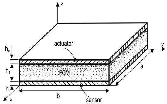
Figure 1. Schematic of sandwich plate.

Heat balance and continuity of temperature at the interfaces are defined by the following relations, respectively:

$$\begin{array}{l}{\lambda }_{zs}\frac{\partial T_s}{\partial z}\left(x,y,h_p\right)={\lambda }_f\frac{\partial T_f}{\partial z}\left(x,y,h_p\right),\\ {\lambda }_f\frac{\partial T_f}{\partial z}\left(x,y,h-h_p\right)={\lambda }_{za}\frac{\partial T_a}{\partial z}\left(x,y,h-h_p\right),\\ T_s\left(x,y,h_p\right)=T_f\left(x,y,h_p\right),\hspace{0.17em}\hspace{1em}{T}_f\left(x,y,h-h_p\right)=T_a\left(x,y,h-h_p\right).\end{array}$$

(3)

2.1. Temperature Field

The three-dimensional steady-state heat conduction equation for the FGM and piezoelectric layers are, respectively [35]:

$${\lambda }_f\frac{{\partial }^2{T}_f}{\partial x^2}+{\lambda }_f\frac{{\partial }^2{T}_f}{\partial y^2}+\frac{\partial {\lambda }_f}{\partial z}\frac{\partial T_f}{\partial z}+{\lambda }_f\frac{{\partial }^2{T}_f}{\partial z^2}=0$$

(4)

$${\lambda }_{xp}\frac{{\partial }^2{T}_p}{\partial x^2}+{\lambda }_{yp}\frac{{\partial }^2{T}_p}{\partial y^2}+{\lambda }_{zp}\frac{{\partial }^2{T}_p}{\partial z^2}=0$$

(5)

2.2. FGM Layer

The three-dimensional equilibrium equations are [36]:

$$\begin{array}{l}{\sigma }_{x,x}+{\tau }_{xy,y}+{\tau }_{xz,z}=0,\\ {\tau }_{xy,x}+{\sigma }_{y,y}+{\tau }_{yz,z}=0,\\ {\tau }_{xz,x}+{\tau }_{yz,y}+{\sigma }_{z,z}=0\end{array}$$

(6)

The strain–displacement relations are [36]:

$$\begin{array}{l}{\epsilon }_x=\frac{\partial u}{\partial x},\hspace{1em}{\epsilon }_y=\frac{\partial v}{\partial y},\hspace{1em}{\epsilon }_z=\frac{\partial w}{\partial z}\\ {\gamma }_{zx}=\frac{\partial u}{\partial z}+\frac{\partial w}{\partial x},\hspace{1em}{\gamma }_{zy}=\frac{\partial v}{\partial z}+\frac{\partial w}{\partial x},\hspace{1em}{\gamma }_{xy}=\frac{\partial u}{\partial y}+\frac{\partial v}{\partial x}\end{array}$$

(7)

Since certain materials exhibit viscoelastic behavior at elevated temperatures, it is essential to account for viscoelasticity to predict the actual response of the materials in such environments. According to the Boltzmann superposition principle, constitutive relations of linear viscoelastic materials are introduced as follows [37]:

$${\sigma }_i={\displaystyle \underset{-\infty }{\overset{t}{\int }}{C}_{ij}\left(t-\tau \right)\frac{d\left({\epsilon }_j\left(\tau \right)-{\alpha }_{j}T\left(\tau \right)\right)}{d\tau }}d\tau$$

(8)

in which $C_{ij}\left(i,j=1,2,\dots ,6\right)$ are the relaxation moduli (see Equation (A1) in the Appendix A). Additionally, ${\sigma }_i\hspace{0.17em}(i=1,2,3)$ represent normal stresses ${\sigma }_x,{\sigma }_y$ and ${\sigma }_z$ while ${\sigma }_i\hspace{0.17em}(i=4,5,6)$ are shear stresses ${\tau }_{xy},{\tau }_{xz}$, and ${\tau }_{yz}$. Likewise, ${\epsilon }_i\hspace{0.17em}(i=1,2,3)$ represent normal strains, ${\epsilon }_x,{\epsilon }_y$, and ${\epsilon }_z$ while ${\epsilon }_i\hspace{0.17em}(i=4,5,6)$ are the shear strains ${\gamma }_{xy},{\gamma }_{xz}$, and ${\gamma }_{yz}$. Before solving the equations, it is convenient to transform Equation (8) into the Laplace domain:

$${\widehat{\sigma }}_i(s)=s{\widehat{C}}_{ij}\left(s\right)\left({\widehat{\epsilon }}_j(s)-{\alpha }_j\widehat{T}\left(s\right)\right)$$

(9)

The Laplace transform of a variable is shown by the caret over it. Substitution of Equation (7) into Equation (9) results in the following stress–displacement relations for the FGM layer.

$$\begin{array}{l}{\widehat{\sigma }}_{fx}=\frac{s\widehat{E}\left(z,s\right)}{\left(1+\nu \right)\left(1-2\nu \right)}\left[\left(1-\nu \right){\widehat{u}}_{f,x}+\nu {\widehat{v}}_{f,y}+\nu {\widehat{w}}_{f,z}\right] -\frac{\alpha \left(z\right)s\widehat{E}\left(z,s\right)}{1-2\nu }{\widehat{T}}_f\\ {\widehat{\sigma }}_{fy}=\frac{s\widehat{E}\left(z,s\right)}{\left(1+\nu \right)\left(1-2\nu \right)}\left[\nu {\widehat{u}}_{f,x}+\left(1-\nu \right){\widehat{v}}_{f,y}+\nu {\widehat{w}}_{f,z}\right]-\frac{\alpha \left(z\right)s\widehat{E}\left(z,s\right)}{1-2\nu }{\widehat{T}}_f\\ {\widehat{\sigma }}_{fz}=\frac{s\widehat{E}\left(z,s\right)}{\left(1+\nu \right)\left(1-2\nu \right)}\left[\nu {\widehat{u}}_{f,x}+\nu {\widehat{v}}_{f,y}+\left(1-\nu \right){\widehat{w}}_{f,z}\right] -\frac{\alpha \left(z\right)s\widehat{E}\left(z,s\right)}{1-2\nu }{\widehat{T}}_f\\ {\widehat{\tau }}_{fxy}=\frac{s\widehat{E}\left(z,s\right)}{2\left(1+\nu \right)}\left({\widehat{u}}_{f,y}+{\widehat{v}}_{f,x}\right), {\widehat{\tau }}_{fxz}=\frac{s\widehat{E}\left(z,s\right)}{2\left(1+\nu \right)}\left({\widehat{u}}_{f,z}+{\widehat{w}}_{f,x}\right) , {\widehat{\tau }}_{fyz}=\frac{s\widehat{E}\left(z,s\right)}{2\left(1+\nu \right)}\left({\widehat{v}}_{f,z}+{\widehat{w}}_{f,y}\right)\end{array}$$

(10)

The subscript $f$ stands for the FGM layer. By assuming a Prony series for the time-dependence of relaxation modulus $E$ and power law function for the thermal expansion $\alpha$ and thermal conductivity coefficients $k$, we can write for $h_p\le z\le \left(h_p+h_f\right)$:

$$\begin{array}{l}E\left(z,t\right)=E_{1m}{(\frac{z}{h_p})}^{m_1}+E_{2m}{(\frac{z}{h_p})}^{m_2}{e}^{\left(-\frac{t}{\tau }\right)}, \alpha \left(z\right)={\alpha }_m{(\frac{z}{h_p})}^{m_3}, k\left(z\right)=k_m{(\frac{z}{h_p})}^{m_4} \\ m_1=\frac{\ln \left(\frac{E_{1c}}{E_{1m}}\right)}{\ln \left(\frac{h_f+h_p}{h_p}\right)};m_2=\frac{\ln \left(\frac{E_{2c}}{E_{2m}}\right)}{\ln \left(\frac{h_f+h_p}{h_p}\right)};m_3=\frac{\ln \left(\frac{{\alpha }_c}{{\alpha }_m}\right)}{\ln \left(\frac{h_f+h_p}{h_p}\right)};m_4=\frac{\ln \left(\frac{{\lambda }_c}{{\lambda }_m}\right)}{\ln \left(\frac{h_f+h_p}{h_p}\right)}\\ \end{array}$$

(11)

$E_{1i}$ and $E_{2i}$$\left(i=m,\mathrm{c}\right)$ are the Prony series parameters for the relaxation modulus; the subscripts $m$ and $c$ denote the metal and ceramic constituents in the FGM layer. $k_i$ and ${\alpha }_i$ represent the thermal conductivity and expansion coefficients of the two constituents, respectively. Two constituents are assumed to have the same relaxation time constant, $\tau$.

State-space differential equations in matrix form are derived from Equations (6) and (10):

$$\frac{d}{dz}{\delta }_f=G_f{\delta }_f+B_f{\widehat{T}}_f$$

(12)

where $G_f$ and $B_f$ are coefficient matrices (see Equations (A2) and (A3) in the Appendix A), and ${\delta }_f=\left[{\widehat{\sigma }}_z,\widehat{u},\widehat{v},\widehat{w},{\widehat{\tau }}_{xz},{\widehat{\tau }}_{yz}\right]$ is the state vector. In-plane stresses are determined using the state variable as:

$$\begin{array}{l}{\widehat{\sigma }}_{fx}=\frac{1}{\left(1-\nu \right)}\left[\nu {\widehat{\sigma }}_{fz}+\frac{s\widehat{E}\left(z,s\right)}{1+\nu }{\widehat{u}}_{f,x}+\frac{s\widehat{E}\left(z,s\right)}{1+\nu }{\widehat{v}}_{f,y}\right]-\frac{s\widehat{E}\left(z,s\right)\alpha \left(z\right)}{1-\nu }{\widehat{T}}_f,\\ {\widehat{\sigma }}_{fy}=\frac{1}{\left(1-\nu \right)}\left[\nu {\widehat{\sigma }}_{fz}+\frac{s\widehat{E}\left(z,s\right)}{1+\nu }{\widehat{u}}_{f,x}+\frac{s\widehat{E}\left(z,s\right)}{1+\nu }{\widehat{v}}_{f,y}\right]-\frac{s\widehat{E}\left(z,s\right)\alpha \left(z\right)}{1-\nu }{\widehat{T}}_f,\\ {\widehat{\tau }}_{fxy}=\frac{s\widehat{E}\left(z,s\right)}{2\left(1+\nu \right)}\left({\widehat{u}}_{f,y}+{\widehat{u}}_{f,x}\right)\end{array}$$

(13)

3. Solution Procedure

3.1. Temperature Gradient

Following the Fourier series expansion satisfies the thermal edge boundary conditions in Equation (2):

$$\mathrm{T}={\displaystyle \sum _{m=1}^{\infty }{\displaystyle \sum _{n=1}^{\infty }{\mathrm{T}}_i(z)\sin \left(p_{m}x\right)\sin \left(p_{n}y\right)}},\hspace{0.17em}\hspace{0.17em}\hspace{0.17em}\hspace{0.17em}\hspace{0.17em}i=a,f,s$$

(14)

where $p_m=\frac{m\pi }{a}$,$p_n=\frac{n\pi }{b}$. Additionally, substituting Equation (14) into Equations (4) and (5) leads to

$$\frac{{\partial }^2{T}_i\left(z\right)}{\partial z^2}-\left(\frac{{\lambda }_{xi}}{{\lambda }_{zi}}{p}_m^2+\frac{{\lambda }_{yi}}{{\lambda }_{zi}}{p}_n^2\right)T_i\left(z\right)=0$$

(15a)

$$\frac{{\partial }^2{T}_f\left(z\right)}{\partial z^2}+\frac{m_4}{z}\frac{\partial T_f\left(z\right)}{\partial z}-\left(p_m^2+p_n^2\right)T_f\left(z\right)=0$$

(15b)

Substituting Equation (14) into Equation (15a) and solving the obtained equations leads to the following relations for the sensor and actuator layers, respectively:

$$T_s\left(z\right)=C_1^s{e}^{{\alpha }_{s}z}+C_2^s{e}^{-{\alpha }_{s}z}$$

(16a)

$$T_a\left(z\right)=C_1^a{e}^{{\alpha }_{a}z}+C_2^a{e}^{-{\alpha }_{a}z}$$

(16b)

where ${\alpha }_s=\sqrt{\frac{{\lambda }_{xs}{p}_m^2+{\lambda }_{ys}{p}_n^2}{{\lambda }_{zs}}}$ and ${\alpha }_a=\sqrt{\frac{{\lambda }_{xa}{p}_m^2+{\lambda }_{ya}{p}_n^2}{{\lambda }_{za}}}$. In addition, the solution of Equation (15b) using Equation (14) after some manipulation can be written as

$$T_f\left(z\right)=C_1^f\frac{J_{{\alpha }_f}\left(i{\beta }_{f}z\right)}{z^{{\alpha }_f}}+C_2^f\frac{Y_{{\alpha }_f}\left(i{\beta }_{f}z\right)}{z^{{\alpha }_f}}$$

(17)

where ${\alpha }_f=\frac{m_4}{2}-\frac{1}{2}$, ${\beta }_f=\sqrt{p_m^2+p_n^2}$, and $i=\sqrt{-1}$. Additionally, the functions $J_{{\alpha }_f}$ and $Y_{{\alpha }_f}$ are Bessel functions of the first and second kind of order ${\alpha }_f$, respectively.

Here $C_1^s$, $C_2^s$, $C_1^a$, $C_2^a$, $C_1^f$, and $C_2^f$ are integration constants that can be computed from surface boundary conditions (z = 0, h) and the continuity of the temperature and the normal component of the heat flux at the interfaces (see Equation (A4) in the Appendix A).

3.2. FGM Layer

We consider simply supported edge boundary conditions with the following relations:

$$\begin{array}{l}{\sigma }_x=0,v=0,w=0,\hspace{0.17em}\mathrm{and}\hspace{0.17em}T=0\hspace{1em}at\hspace{1em}x=0,a\\ {\sigma }_y=0,u=0,w=0,\hspace{0.17em}\mathrm{and}\hspace{0.17em}T=0\hspace{1em}at\hspace{1em}y=0,b\end{array}$$

(18)

These boundary conditions are identically satisfied by the following Fourier series expansions for the stresses, displacements, and temperature along the in-plane coordinates

$$\begin{array}{l}{\widehat{u}}_f={\displaystyle \sum _{m=1}^{\infty }{\displaystyle \sum _{n=1}^{\infty }{\widehat{u}}_f{}^{\prime }(z)\cos \left(p_{m}x\right)\sin \left(p_{n}y\right)}}\hspace{1em}\hspace{1em}\hspace{1em}{\widehat{v}}_f={\displaystyle \sum _{m=1}^{\infty }{\displaystyle \sum _{n=1}^{\infty }{\widehat{v}}_f{}^{\prime }(z)\sin \left(p_{m}x\right)\cos \left(p_{n}y\right)}}\\ {\widehat{w}}_f={\displaystyle \sum _{m=1}^{\infty }{\displaystyle \sum _{n=1}^{\infty }{\widehat{w}}_f{}^{\prime }(z)\sin \left(p_{m}x\right)\sin \left(p_{n}y\right)}}\hspace{1em}\hspace{1em}\hspace{1em}{\widehat{\sigma }}_{fz}={\displaystyle \sum _{m=1}^{\infty }{\displaystyle \sum _{n=1}^{\infty }{\widehat{\sigma }}^{\prime }{}_{fz}(z)\sin \left(p_{m}x\right)\sin \left(p_{n}y\right)}}\\ {\widehat{\tau }}_{fyz}={\displaystyle \sum _{m=1}^{\infty }{\displaystyle \sum _{n=1}^{\infty }{\widehat{\tau }}^{\prime }{}_{fyz}(z)\sin \left(p_{m}x\right)\cos \left(p_{n}y\right)}}\hspace{1em}\hspace{1em}{\widehat{\tau }}_{fxz}={\displaystyle \sum _{m=1}^{\infty }{\displaystyle \sum _{n=1}^{\infty }{\widehat{\tau }}^{\prime }{}_{fxz}(z)\cos \left(p_{m}x\right)\sin \left(p_{n}y\right)}}\\ {\widehat{\sigma }}_{fx}={\displaystyle \sum _{m=1}^{\infty }{\displaystyle \sum _{n=1}^{\infty }{\widehat{\sigma }}_{fx}{}^{\prime }(z)\sin \left(p_{m}x\right)\sin \left(p_{n}y\right)}}\hspace{1em}\hspace{1em}\hspace{1em}{\widehat{\sigma }}_{fy}={\displaystyle \sum _{m=1}^{\infty }{\displaystyle \sum _{n=1}^{\infty }{\widehat{\sigma }}^{\prime }{}_{fy}(z)\sin \left(p_{m}x\right)\sin \left(p_{n}y\right)}}\\ {\widehat{\tau }}_{fxy}={\displaystyle \sum _{m=1}^{\infty }{\displaystyle \sum _{n=1}^{\infty }{\widehat{\tau }}^{\prime }{}_{fxy}(z)\cos \left(p_{m}x\right)\cos \left(p_{n}y\right)}}\hspace{1em}\hspace{1em}\widehat{T_f}={\displaystyle \sum _{m=1}^{\infty }{\displaystyle \sum _{n=1}^{\infty }\widehat{T_f}{}^{\prime }(z)\sin \left(p_{m}x\right)\sin \left(p_{n}y\right)}}\end{array}$$

(19)

with $p_m=\frac{m\pi }{a}$, $p_n=\frac{n\pi }{b}$. For convenience, non-dimensional quantities are introduced:

$$\begin{array}{l}\overline{T}=\frac{{\alpha }^{*}T}{p},\hspace{1em}\left({\overline{u}}_f,{\overline{v}}_f,{\overline{w}}_f\right)=\left({\widehat{u}}_f^{\prime },{\widehat{v}}_f^{\prime },{\widehat{w}}_f^{\prime }\right)\frac{1}{ph},\hspace{1em}\hspace{1em}\overline{E}=\frac{\widehat{E}}{k^{*}}\\ \left({\overline{\sigma }}_{fx},{\overline{\sigma }}_{fy},{\overline{\sigma }}_{fz},{\overline{\tau }}_{fzx},{\overline{\tau }}_{fzy},{\overline{\tau }}_{fxy}\right)=\left({\widehat{\sigma }}^{\prime }{}_{fx},{\widehat{\sigma }}^{\prime }{}_{fy},{\widehat{\sigma }}^{\prime }{}_{fz},{\widehat{\tau }}^{\prime }{}_{fzx},{\widehat{\tau }}^{\prime }{}_{fzy},{\widehat{\tau }}^{\prime }{}_{fxy}\right)\frac{1}{p{k}^{*}}\\ \overline{x}=\frac{x}{h}, \overline{y}=\frac{y}{h} , \overline{z}=\frac{z}{h}\hspace{1em}, {\overline{p}}_m=a{p}_m,\hspace{1em}\hspace{1em}{\overline{p}}_n=b{p}_n\end{array}$$

(20)

Here $k^{*}=1\hspace{0.17em}GPa$ and ${\alpha }^{*}={10}^{-6}/K$ are the scale factors, and $p={\alpha }^{*}{T}_o$.

Using Equations (19) and (20) in Equation (12) results in the following non-dimensional state-space equation

$$\frac{d}{d\overline{z}}{\overline{\delta }}_f={\overline{G}}_f{\overline{\delta }}_f+{\overline{B}}_f{\overline{T}}_f$$

(21)

where ${\overline{\delta }}_f={\left[{\overline{\sigma }}_{fz},{\overline{u}}_f,{\overline{v}}_f,{\overline{w}}_f,{\overline{\tau }}_{fxz},{\overline{\tau }}_{fyz}\right]}^T$ is the state vector in the FGM core and ${\overline{G}}_f$ and ${\overline{B}}_f$ are a non-dimensional square matrix and a vector of coefficients (see Equations (A5) and (A6) in the Appendix A). The non-dimensional in-plane stresses can be computed from the non-dimensional state variables as

$$\left\{\begin{array}{c}{\overline{\sigma }}_{fx}\\ {\overline{\sigma }}_{fy}\\ {\overline{\tau }}_{xy}\end{array}\right\}=\left[\overline{F}\right]\left\{\begin{array}{c}{\overline{\sigma }}_{fz}\\ {\overline{u}}_f\\ {\overline{v}}_f\\ {\overline{T}}_f\end{array}\right\}$$

(22)

in which $\overline{F}$ is a coefficient matrix (see Equation (A7) in the Appendix A).

Since the components of the coefficient matrix ${\overline{G}}_f$ depend on the thickness coordinate z, it is not possible to solve Equation (21) analytically. By dividing the FGM layer into $N_f$ fictitious thin layers with a negligible variation of the material properties through their thickness, the ${\overline{G}}_f$ matrix is converted to a constant matrix for each of these fictitious layers and the following solution to Equation (21) is derived for the $k^{th}$ layer, with $k=1,2,\dots ,N_f$:

$$\left[e^{-{\overline{G}}_{f_k}{\overline{z}}_{k-1}}{\overline{\delta }}_{f_{0k}}+{\displaystyle {\int }_{{\overline{z}}_{k-1}}^{{\overline{z}}_k}{e}^{-{\overline{G}}_{f_k}\eta }}{\overline{B}}_{f_k}\left(\eta \right){\overline{T}}_f\left(\eta \right)d\eta \right],\hspace{1em}{\overline{z}}_{k-1}\le \overline{z}\le {\overline{z}}_k$$

(23)

in which

$${\overline{z}}_{k-1}={\overline{h}}_p+\frac{\left(k-1\right){\overline{h}}_f}{N_f},\hspace{1em}{\overline{z}}_k={\overline{h}}_p+\frac{k{\overline{h}}_f}{N_f},\hspace{1em}{\overline{\delta }}_{f_{0k}}={\overline{\delta }}_{f_k}\left(\overline{z}={\overline{z}}_{k-1}\right)\hspace{1em}$$

Computing Equation (23) at the upper side of the k-th layer with z = ${\overline{z}}_k$ finds

$${\overline{\delta }}_{f_k}\left({\overline{z}}_k\right)=M_k{\overline{\delta }}_{f_{0k}}+I_k$$

(24)

where $M_k=e^{\left({\overline{G}}_{f_k}\frac{{\overline{h}}_f}{N_f}\right)}$ and $I_k=e^{{\overline{G}}_{f_k}{\overline{z}}_k}{\displaystyle {\int }_{{\overline{z}}_{k-1}}^{{\overline{z}}_k}{e}^{-{\overline{G}}_{f_k}\eta }}{\overline{B}}_{f_k}\left(\eta \right){\overline{T}}_f\left(\eta \right)d\eta$, relating the state vector at the upper side of the layer with the one at the lower side of the layer. From the continuity of displacements and transverse normal and shear stresses at the interface of each of two adjacent fictitious layers, it is possible to determine the relation between the state vector at the top, ${\overline{\delta }}_{f_{\left(\left(h_p+h_f\right)/h\right)}}$, and bottom, ${\overline{\delta }}_{f_0}$, surfaces of the FGM layer:

$${\overline{\delta }}_{f_{\left(\left(h_p+h_f\right)/h\right)}}=M_f{\overline{\delta }}_{f_0}+I$$

(25)

where $M_k={\displaystyle {\prod }_{k=N_f}^1{e}^{\left({\overline{G}}_{fk}\frac{{\overline{h}}_f}{N_f}\right)}}$ and $I={\displaystyle \sum _{i=1}^{N_f-1}\left({\displaystyle \prod _{k=i+1}^{N_f}{M}_k{I}_i}\right)+I_{N_f}}$.

3.3. Piezoelectric Layer

The constitutive relations for the orthotropic piezoelectric layers are [20]

$${\sigma }_p=C_p{\epsilon }_p-e^T{E}_p-\beta {\widehat{T}}_p$$

(26)

$$D=e{\epsilon }_p+\eta E_p+P_3{\widehat{T}}_p$$

(27)

where $C_p,\eta$ and $e$ are the elasticity matrix, the permittivity matrix, and the piezoelectric coefficient matrix; $\beta$ is the matrix of stress–temperature coefficients; and $P_3$ is the pyroelectric coefficient matrix. The specific form for the piezoelectric materials under consideration is given in Equation (A8) in the Appendix A. Stresses ${\sigma }_p$, strains ${\epsilon }_p$, electric displacements $D$, and electric field components ${\mathrm{E}}_p$ are

$${\sigma }_p=\left[\begin{array}{cccccc}{\widehat{\sigma }}_x& {\widehat{\sigma }}_y& {\widehat{\sigma }}_z& {\widehat{\tau }}_{xz}& {\widehat{\tau }}_{yz}& {\widehat{\tau }}_{xy}\end{array}\right],\hspace{1em}{\epsilon }_p=\left[\begin{array}{cccccc}{\widehat{\epsilon }}_{\mathrm{x}}& {\widehat{\epsilon }}_y& {\widehat{\epsilon }}_z& {\widehat{\gamma }}_{xz}& {\widehat{\gamma }}_{yz}& {\widehat{\gamma }}_{xy}\end{array}\right]$$

$$D={\left[\begin{array}{ccc}{D}_x& D_y& D_z\end{array}\right]}^T,\hspace{1em}{E}_p={\left[\begin{array}{ccc}{E}_x& E_y& E_z\end{array}\right]}^T$$

Equilibrium equations for the piezoelectric layers are the same as for the FGM layer (Equation (6)). The charge equation of electrostatics for the non-conducting piezoelectric layers is [20]

$$D_{x,x}+D_{y,y}+D_{z,z}=0$$

(28)

Moreover, the electric field vector is the negative gradient of the electric potential as [20]:

$$E_x=-{\psi }_{,x} , E_y=-{\psi }_{,y} , E_z=-{\psi }_{,z}$$

(29)

The simply supported boundary condition relations for piezoelectric layers are the same as Equation (18), along with the following relations for electric potential $\psi$:

$$\psi =0,\hspace{1em} at x=0,a \mathrm{and} y=0,b$$

(30)

Combining Equations (26)–(29) and Equation (6) results in the following state-space differential equation in the Laplace domain:

$$\frac{d}{dz}{\delta }_p=G_p{\delta }_p+B_p{\widehat{T}}_p$$

(31)

where ${\delta }_P={\left\{\begin{array}{cccc}\begin{array}{cccc}\begin{array}{cc}{\widehat{\sigma }}_{pz}& {\widehat{u}}_p\end{array}& {\widehat{v}}_p& {\widehat{w}}_p& {\widehat{\tau }}_{pzx}\end{array}& {\widehat{\tau }}_{pzy}& {\widehat{D}}_z& \widehat{\psi }\end{array}\right\}}^T$; $G_p$ and $B_p$ represent the coefficient matrix and vector, respectively (Equations (A9) and (A10) in the Appendix A).

The following dimensionless quantities and those introduced in Equation (20) are used for the piezoelectric layers:

$$\begin{array}{l}({\overline{E}}_x,{\overline{E}}_y,{\overline{E}}_z)=(E_x,E_y,E_z)\frac{\left|d_1\right|}{{\alpha }^{*}{T}_o}, \left({\overline{D}}_x,{\overline{D}}_y,{\overline{D}}_z\right)=\left({\widehat{D}}^{\prime }{}_x,{\widehat{D}}^{\prime }{}_y,{\widehat{D}}^{\prime }{}_z\right)\frac{1}{p{k}^{*}\left|d_1\right|}\\ \left({\overline{\eta }}_1,{\overline{\eta }}_2,{\overline{\eta }}_3\right)=\left({\eta }_1,{\eta }_2,{\eta }_3\right)\frac{1}{k^{*}{\left|d_1\right|}^2},\hspace{1em}\left({\overline{e}}_1,{\overline{e}}_2,{\overline{e}}_3,{\overline{e}}_4,{\overline{e}}_5\right)=\left(e_1,e_2,e_3,e_4,e_5\right)\frac{1}{k^{*}\left|d_1\right|}\\ {\widehat{\psi }}^{\prime }=\frac{\left|d_1\right|\overline{\psi }}{({\alpha }^{*}{T}_{o}h)},\hspace{1em}\left({\overline{\beta }}_x,{\overline{\beta }}_y,{\overline{\beta }}_z\right)=\left({\beta }_x,{\beta }_y,{\beta }_z\right)\frac{1}{k^{*}{\alpha }^{*}},\hspace{1em}{\overline{C}}_{ij}=\frac{C_{ij}}{k^{*}},\hspace{1em}{\overline{p}}_3=\frac{p_3}{k^{*}{\alpha }^{*}\left|d_1\right|}\end{array}$$

(32)

The Fourier series expansion, Equation (19), can be utilized for the piezoelectric layers by changing subscript “f” to “i” and for the electric potential and electric displacement they are as the following:

$${\widehat{\psi }}_i={\displaystyle \sum _{m=1}^{\infty }{\displaystyle \sum _{n=1}^{\infty }{\widehat{\psi }}_i{}^{\prime }(z)\sin \left(p_{m}x\right)\sin \left(p_{n}y\right)}},\hspace{1em}{\widehat{D}}_i{}_z={\displaystyle \sum _{m=1}^{\infty }{\displaystyle \sum _{n=1}^{\infty }{\widehat{D}}_i{{}^{\prime }}_z(z)\sin \left(p_{m}x\right)\sin \left(p_{n}y\right)}};i=a,s$$

(33)

Dimensionless state-space differential matrix equations are determined via substitution of Equations (19), (32), and (33) into Equation (31):

$$\frac{d}{dz}{\overline{\delta }}_P={\overline{G}}_P{\overline{\delta }}_P+{\overline{B}}_p{\overline{T}}_p$$

(34)

where ${\overline{\delta }}_P={\left\{\begin{array}{cccc}\begin{array}{cccc}\begin{array}{cc}{\overline{\sigma }}_{pz}& {\overline{u}}_p\end{array}& {\overline{v}}_p{}_{}& {\overline{w}}_p& {\overline{\tau }}_{pzx}\end{array}& {\overline{\tau }}_{pzy}& {\overline{D}}_z& \overline{\psi }\end{array}\right\}}^T$ is the state vector; the matrices ${\overline{G}}_P$ and ${\overline{B}}_p$ are coefficient matrix and vector, respectively (Equations (A11) and (A12) in the Appendix A).

Dimensionless in-plane stresses can be determined in terms of state variables

$$\left\{\begin{array}{c}{\overline{\sigma }}_{px}\\ {\overline{\sigma }}_{py}\\ {\overline{\tau }}_{pxy}\end{array}\right\}=\left[{\overline{F}}_p\right]\left\{\begin{array}{c}{\overline{\sigma }}_{pz}\\ {\overline{u}}_p\\ {\overline{v}}_p\\ \begin{array}{l}{\overline{D}}_z\\ {\overline{T}}_p\end{array}\end{array}\right\}$$

(35)

Here ${\overline{F}}_p$ is the coefficient matrix introduced in Equation (A13) in the Appendix A.

The general solutions for Equation (34) for the sensor and actuator layers are, respectively:

$${\overline{\delta }}_s\left(\overline{z}\right)=e^{{\overline{G}}_s\overline{z}}\left[\overline{\delta }\left(0\right)+{\displaystyle {\int }_0^{\overline{z}}{e}^{-{\overline{G}}_s\eta }}{\overline{B}}_p\left(\eta \right){\overline{T}}_s\left(\eta \right)d\eta \right],\hspace{1em}at\hspace{0.17em}0\le \overline{z}\le h_p/h$$

(36)

$$\begin{array}{l}{\overline{\delta }}_a\left(\overline{z}\right)=e^{{\overline{G}}_a\overline{z}}\left[e^{-{\overline{G}}_a\left(\frac{h_p+h_f}{h}\right)}{\overline{\delta }}_a\left(\frac{h_p+h_f}{h}\right)+{\displaystyle {\int }_{\frac{h_p+h_f}{h}}^{\overline{z}}{e}^{-{\overline{G}}_a\eta }}{\overline{B}}_p\left(\eta \right){\overline{T}}_a\left(\eta \right)d\eta \right],\\ at\hspace{0.17em}\left(h_p+h_f\right)/h\le \overline{z}\le h/h\end{array}$$

(37)

At the above surfaces of actuator and sensor layers, Equations (36) and (37) are, respectively,

$${\overline{\delta }}_a\left(h/h\right)=M^a{\overline{\delta }}_a\left(\left(h_p+h_f\right)/h\right)+{M^{\prime }}^a{N}^a$$

(38)

$${\overline{\delta }}_s\left(h_p\right)=M^s\left({\overline{\delta }}_s\left(0\right)+N^s\right)$$

(39)

in which

$$M^a=e^{\left[{\overline{G}}_a{h}_p/h\right]},\hspace{1em}{M^{\prime }}^a=e^{\left[{\overline{G}}_{a}h/h\right]},\hspace{1em}{N}^a={\displaystyle {\int }_{\left(h_p+h_f\right)/h}^{h/h}{e}^{-{\overline{G}}_a\eta }}{\overline{B}}_a\left(\eta \right){\overline{T}}_a\left(\eta \right)d\eta$$

$$M^s=e^{\left[{\overline{G}}_s{h}_p/h\right]},\hspace{1em}{N}^s={\displaystyle {\int }_0^{h_p/h}{e}^{-{\overline{G}}_s\eta }}{\overline{B}}_s\left(\eta \right){\overline{T}}_s\left(\eta \right)d\eta$$

Electric displacement at the lower surface of the actuator layer is calculated by using Equation (38) [38]:

$$\begin{array}{l}{\overline{D}}_z\left(\left(h_p+h_f\right)/h\right)=\frac{1}{m_{87}^a}\left[\overline{\psi }\left(h/h\right)-\left[m_{8j}^a\right]{\overline{\delta }}^m\left(\left(h_p+h_f\right)/h\right)-\left[m_{8k}^{\prime a}\right]\right],\\ j=1,\dots ,6,\hspace{1em}k=1,\dots ,8.\end{array}$$

(40)

where $m_{8j}^a$ represents the element at the 8th row and jth column of the $M^a$ matrix and ${\overline{\delta }}^m\left(\left(h_p+h_f\right)/h\right)$ is the mechanical part of the state vector of the actuator at its interface with the viscoelastic layer, ${\overline{\delta }}_p{}^m={\left\{{\overline{\sigma }}_{pz},{\overline{u}}_p,{\overline{v}}_p,{\overline{w}}_p,{\overline{\tau }}_{pzx},{\overline{\tau }}_{pzy}\right\}}^T$.

Inserting $\overline{\psi }\left(\left(h_p+h_f\right)/h\right)=0$ Equation (40), into Equation (38) yields:

$${\overline{\delta }}^m\left(h\right)=T_a{\overline{\delta }}^m\left(\left(h_p+h_f\right)/h\right)+C_a+B_a{N}^a$$

(41)

where

$$\begin{array}{l}{T}_a=\left[\left[m_{ij}^a\right]-\left\{m_{i7}^a\right\}\frac{1}{m_{87}^a}\left[m_{8j}^a\right]\right],\hspace{1em}{C}_a=\left\{m_{i7}^a\right\}\frac{\overline{\psi }\left(h\right)}{m_{87}^a},\\ B_a=[m_{ik}^{\prime a}]-\left\{m_{i7}^a\right\}\frac{1}{m_{87}^a}\left[m_{8k}^a\right],\hspace{1em}i=1,2,\dots ,6,\hspace{1em}j=1,2,\dots ,6,\hspace{1em}k=1,2,\dots ,8.\end{array}$$

Using Equation (39), the electric potential $\psi$ at the lower surface of the sensor can be derived as:

$$\overline{\psi }\left(0\right)=\frac{1}{m_{88}^s}\left(\left[m_{8j}^s\right]{\overline{\delta }}^m\left(0\right)+N_s\right),j=1,2,\dots ,6.$$

(42)

Substitution of $D_z=0$ and inserting Equation (42) into Equation (39) results in

$${\overline{\delta }}_p^m\left(h\right)=T_s{\overline{\delta }}_p^m\left(0\right)+B_s{N}_s,$$

(43)

where

$$\begin{array}{l}{T}_s=\left[\left[m_{ij}^s\right]-\left\{m_{i8}^s\right\}\frac{1}{m_{88}^s}\left[m_{8j}^s\right]\right],\\ B_s=\left[m_{ij}^s\right]-\left\{m_{i8}^s\right\}\frac{1}{m_{88}^s}\left[m_{8k}^s\right],\hspace{1em}i=1,2,\dots ,6,\hspace{1em}j=1,2,\dots ,6,\hspace{1em}k=1,2,\dots ,8\end{array}$$

Since the transverse normal and shear stresses and displacements at the interfaces of the actuator, FGM, and sensor are continuous, from Equations (25), (41) and (43), the mechanical state variables at the top surface relate to those at the bottom surface with the following matrix equation

$${\overline{\delta }}^m\left(h\right)=S{\overline{\delta }}^m\left(0\right)+Y$$

(44)

where $S=T_{a}M{T}_s$.

Applying surface traction boundary conditions at the bottom and top surfaces to Equation (44) leads to the following equations

$$\left[\begin{array}{ccc}{s}_{12}& s_{13}& s_{14}\\ s_{52}& s_{53}& s_{54}\\ s_{62}& s_{63}& s_{64}\end{array}\right]\left\{\begin{array}{c}{\overline{u}}_0\\ {\overline{v}}_0\\ {\overline{w}}_0\end{array}\right\}=\left\{\begin{array}{c}Y\left(1\right)\\ Y\left(5\right)\\ Y\left(6\right)\end{array}\right\}$$

(45)

By solving Equation (45), the displacement components at the bottom surface of the sensor layer $\left[\begin{array}{ccc}{\overline{u}}_0& {\overline{v}}_0& {\overline{w}}_0\end{array}\right]$ are obtained; then, using Equations (23), (26), and (37), mechanical and electrical state variables can be computed. Finally, modified Dubner’s and Abats’s numerical techniques are employed to transform the displacement and stress fields from Laplace to the time domain [39].

4. Numerical Results and Discussion

For numerical illustration, a simply supported viscoelastic FGM plate attached to piezoelectric layers is considered. The thermo-mechanical properties of the piezoelectric layers are presented in Table 1 [21,38].

Table 1. Material properties of the piezoelectric sensor and actuator layers [21,38].

Elasticity Constant [109 Nm−2]	${\mathit{Q}}_{11}$	${\mathit{Q}}_{12}$	${\mathit{Q}}_{13}$	${\mathit{Q}}_{22}$	${\mathit{Q}}_{23}$	${\mathit{Q}}_{33}$	${\mathit{Q}}_{44}$	${\mathit{Q}}_{55}$	${\mathit{Q}}_{66}$
Sensor (PZT-4)	139	78	74	139	74	115	25.6	25.6	30.5
Actuator (Ba2 NaNb5 O15)	239	104	50	274	52	135	65	66	76
Piezoelectric coefficients [coul·m−2]	${\epsilon }_{31}$	${\epsilon }_{32}$	${\epsilon }_{33}$	${\epsilon }_{24}$	${\epsilon }_{15}$
Sensor	−5.2	−5.2	15.1	12.7	12.7
Actuator	−0.4	−0.3	4.3	3.4	2.8
Dielectric constants [10−9 farads·m−1]	η1		η2	η3
Sensor	6.5		6.5	5.6
Actuator	1.96		2.01	0.28
Thermal conductivity $[\mathrm{W}/(\mathrm{mK}\left)\right]$	${\lambda }_x={\lambda }_y$		${\lambda }_z$
Sensor	2.1		3.15
Actuator	8.6		12.9
Thermal expansion [$[1/\mathrm{K}]\times {10}^{-6}$]	${\alpha }_x={\alpha }_y$		${\alpha }_z$
Sensor	1.97		2.62
Actuator	4.39		2.45
Piezoelectric modulus pyroelectric constant:	$d_1$		$p_3$
Sensor	−3.92		5.4
Actuator	−3.92		5.4

The relaxation time constant, Poisson’s ratio, and the parameters for the Prony series are [40]:

$$\begin{array}{l}{E}_{1m}=70\hspace{0.17em}GPa,\hspace{1em}{E}_{2m}=105\hspace{0.17em}GPa,\hspace{1em}{E}_{1c}=380\hspace{0.17em}GPa,\hspace{1em}{E}_{2c}=570\hspace{0.17em}GPa, {\alpha }_c=8.4\times {10}^{-6}\frac{1}{{}^{°}K}, \\ {\alpha }_m=22.2\times {10}^{-6}\frac{1}{{}^{°}K},{\lambda }_m=205\frac{W}{m^{°}K},\hspace{1em}{\lambda }_c=35\frac{W}{m^{°}K},\tau =5s, v=0.3 .\hspace{1em}\end{array}$$

It is worth noting that all the presented results are the maximum values within the domain of the plate that are computed at $t=2 \mathrm{s}$. The geometrical dimensions of the plate and the bottom and top surface temperature of the plate are introduced as:

$$a/b=1.5,\hspace{1em}a/h=10,\hspace{1em}h/h_p=25,\hspace{0.17em}{V}_0=0,\hspace{0.17em}{T}_i=400\hspace{0.17em}K, \mathrm{and} T_o=600\hspace{0.17em}K.\hspace{1em}$$

At first, a convergence study for the proposed analytical solution is conducted for normal transverse stress, deflection, and latitudinal displacement along the thickness direction for different values of half-wave numbers ($m, n$) and plotted in Figure 2a–c. As the figures show, transverse quantities are more affected by the half-wave numbers. Additionally, the figures indicate that by increasing the half-wave numbers up to $m=n=11$, transverse normal stress, deflection, and latitudinal displacement perfectly converge to their corresponding constant values. This matter clearly shows the high convergence rate of the Fourier series technique. In other words, this shows the optimum pace of convergence for the applied solution, and it means that this method requires comparatively lower computational effort, which is highly essential for time-variant analysis of the thermoelastic response of the sandwich structure.

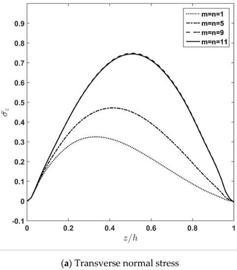
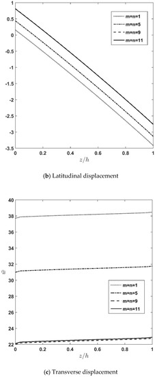
Figure 2. Through-thickness distribution of transverse normal stress, latitudinal displacement, and deflection of plate for different half wave numbers (m, n).

Moreover, the consequence of increasing the number of fictitious layers constituting the FGM part of the sandwich plate on the convergence of stresses and displacement along the thickness direction is presented in Figure 3a–c. Scrutinizing the diagrams shown in this figure reveals that increasing the number of fictitious layers for N > 10 has infinitesimal effect on their trend. In other words, considering N = 10 as the total number of fictitious layers guarantees the acceptable degree of stability for the applied solution. Accordingly, further computations in this research would be carried out by considering N = 10 as the minimum number of fictitious layers of FGM required for obtaining a stable rate of convergence.

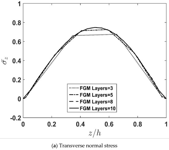
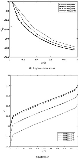
Figure 3. Effect of fictitious layer number of FGM layer on through-thickness distribution of dimensionless normal and shear stresses and deformation for the FG core.

To carry out the validation of the present formulation, numerical results for dimensionless displacements and stresses of thick and thin FG rectangular plates subjected to a temperature gradient were computed and presented in Table 2 to compare with the published results. Comparison of the present results with the results reported by Refs. [38,41,42] shows that the corresponding discrepancy between the present results with those of the mentioned references is less than 1%. Accordingly, Table 2 reveals a perfect agreement between the results of the current study and the results reported in the high-quality studies published previously. To this end, it can be said that the method and solution employed in this study are of high accuracy. Finally, it is essential to notice that the discrepancy between the current results with Ref. [41] is due to the extended unified formulation used in the mentioned reference.

Table 2. Numerical result displacements for FGM square plate under a thermal load.

	$\frac{\mathit{a}}{\mathit{h}}=4$				$\frac{\mathit{a}}{\mathit{h}}=50$
	[41]	[42]	[38]	Present	[41]	[42]	[38]	Present
$\overline{w}\left(h\right)$	3.043	3.043	3.0431	3.043	28.54	28.53	28.53	28.53
$\overline{w}\left(\frac{h}{2}\right)$	2.144	2.143	2.1443	2.143	28.46	28.45	28.448	28.45
$\overline{w}\left(0\right)$	1.901	1.901	1.9012	1.900	28.44	28.43	28.432	28.43
$\overline{u}\left(h\right)$	−1.681	−1.681	−1.681	−1.681	−1.703	−1.703	−1.7027	−1.703
$\overline{u}\left(\frac{h}{2}\right)$	−0.6822	−0.6822	−0.6823	−0.6860	−0.8080	−0.8081	−0.8081	−0.808
$\overline{u}\left(0\right)$	0.08266	0.08240	0.08242	0.08241	0.08553	0.08528	0.08527	−0.08552
${\overline{\sigma }}_x\left(h\right)$	−1018	−1018	−1018	−1018	−1003	−1003	−1003	−1003
${\overline{\sigma }}_x\left(\frac{h}{2}\right)$	−204.7	−204.8	−204.82	−204.821	−251.2	−251.2	−251.208	−251.2084
${\overline{\sigma }}_x\left(0\right)$	−74.03	−73.53	−73.525	−73.525	−76.59	−76.10	−76.12	−76.1239
${\tau }_{xz}\left(\frac{h}{2}\right)$	4.203	4.186	4.1875	4.1875	0.3135	0.3122	0.3123	0.3123
${\overline{\sigma }}_z\left(\frac{h}{2}\right)$	6.300	6.217	6.23	6.2342	0.1178	0.04067	0.04051	0.4051

After the convergence study and the validation analysis of the utilized methods are performed, it is time to present a parametric study regarding the effects of length-to-thickness ratio, $a/h$; FGM layer thickness to piezoelectric layers thickness, $h/h_p$; outer surface temperature, $T_o$; and relaxation time constant, $\tau$, on the thermo-visco-elastic behavior of an FGM plate surrounded by piezoelectric layers.

Figure 4a–d depicts through-thickness distribution of the axial normal stress ${\overline{\sigma }}_x$, transverse shear stress ${\overline{\tau }}_{zx}$, and deflection $\overline{w}$ for different length-to-thickness-ratios $a/h$. According to the figures and as expected, increasing $a/h$ causes a decrease in the stiffness of the plate, and accordingly, the stresses decrease. Moreover, it is seen that the rate of variation decreases by increasing the value of the length-to-thickness ratio. In other words, according to Figure 4a, it can be seen that increasing the value of $a/h$ from 10 to 20 causes the maximum value of the axial normal stress, ${\overline{\sigma }}_x$, to change from 1692 to 544. Meanwhile, increasing the value of $a/h$ from 20 to 40 causes the maximum value of the axial normal stress, ${\overline{\sigma }}_x$, to be changed from 544 to 427. Additionally, according to Figure 4b, it can be stated that increasing the value of $a/h$ from 10 to 20 causes the maximum value of the transverse shear stress, ${\overline{\tau }}_{zx}$, to change from 48.129 to 8.352. Meanwhile, increasing the value of $a/h$ from 20 to 40 causes the maximum value of the transverse shear stress, ${\overline{\tau }}_{zx}$, to change from 8.352 to 2.967.

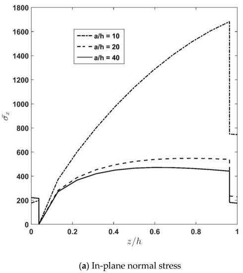
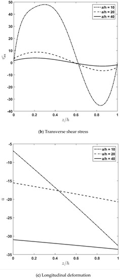
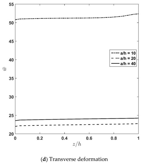
Figure 4. Influence of aspect ratio, $a/h$, on in-plane normal stress, transverse shear stress, and longitudinal and transverse displacement.

The influence of the total thickness to piezoelectric thickness ratio, $h/h_p$, while the total thickness is kept constant is illustrated in Figure 5a–c. As the figures show, decreasing the piezoelectric layer thickness applies a more considerable effect on the normal transversal stress ${\overline{\sigma }}_z$. Additionally, it can be observed that decreasing the piezoelectric layer thickness causes the stresses and displacement to converge to their corresponding constant values. In this regard, the difference between the thermoelastic response of the system for $h/h_p$ = 100 and $h/h_p$ = 150 is lower than 3%. As a conclusion, it can be stated that decreasing the thickness of the piezoelectric layers causes a decrease in their effect on the stress and deflection variation of the system when $h/h_p\ge 150$. It is concluded that in the absence of an applied voltage for $h/h_p\ge 150$, the effect of the piezoelectric thickness on the thermo-visco-elastic behavior becomes negligible.

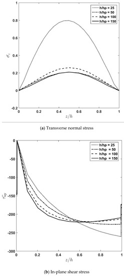
Figure 5. Effect of piezoelectric thickness variation on through-thickness distribution of dimensionless transverse normal stress, in-plane shear stress, and longitudinal displacement.

Table 3 presents the variation of the stresses and deflection across the thickness for different applied temperatures. According to this table, it is observed that as $T_o$ increases, ${\overline{\tau }}_{xy}$ and ${\overline{\sigma }}_z$ decrease, whereas the deflection increases. Moreover, it is observed that the influence of a temperature difference in the lower region is greater than that for the upper region, which is due to the thermal barrier behavior of the FGM core at the upper surface.

Table 3. Effect of different outer surface temperature, $T_o$, on the transverse normal and in-plane shear stresses, as well as longitudinal displacement and transverse displacements.

	${\mathit{T}}_{\mathit{o}}$	$\mathit{z}/\mathit{h}$
		0	0.2	0.4	0.6	0.8	1
$\overline{u}\left(0,\frac{b}{2}\right)$	600	−20.620	−20.850	−21.100	−21.392	−21.706	−22.040
	800	−15.547	−16.507	−17.509	−18.574	−19.576	−20.704
	900	−13.856	−15.088	−16.403	−17.635	−18.929	−20.265
$\overline{w}\left(\frac{a}{2},\frac{b}{2}\right)$	600	5.6785	6.0438	6.1482	6.3048	6.4092	6.5658
	800	22.015	22.276	22.380	22.484	22.589	22.797
	900	27.443	27.704	27.756	27.860	28.017	28.173
${\overline{\sigma }}_z\left(\frac{a}{2},\frac{b}{2}\right)$	600	0	0.4945	0.7732	0.7438	0.4281	0
	800	0	0.4155	0.7031	0.7167	0.4301	0
	900	0	0.3892	0.6798	0.7076	0.4307	0
${\tau }_{xy}\left(0,0\right)$	600	−199.79	−181.63	−239.87	−257.41	−258.66	−202.92
	800	−137.79	−124.63	−187.27	−225.47	−248.64	−199.16
	900	−117.12	−105.22	−169.73	−214.82	−246.14	−197.91

For different values of the relaxation time constant $\tau$, the distribution of latitudinal and transverse displacements as well as transverse normal and shear stresses along the thickness are computed and plotted in Figure 6a–d. The figures show that increasing the relaxation time constant causes stress components to increase and displacement components to decrease due to the increase in the visco-elastic plate stiffness compared to the elastic one. Furthermore, it can be observed that the value of the relaxation time constant, $\tau$, is more considerable in the trend of displacement terms compared to stresses. Additionally, one can observe from Figure 6a that increasing $\tau$ from 2 (s) to 6 (s) applies more significant impact on the transverse normal stress ${\overline{\sigma }}_z$ compared with the change made on the value of ${\overline{\sigma }}_z$ when $\tau$ changes from 6 (s) to 10 (s). Accordingly, it can be stated that ${\overline{\sigma }}_z$ converges to the constant value when $\tau$ reaches its upper bound. In other words, the effect of increasing $\tau$ on the transverse normal stress terms fades for higher values of $\tau$.

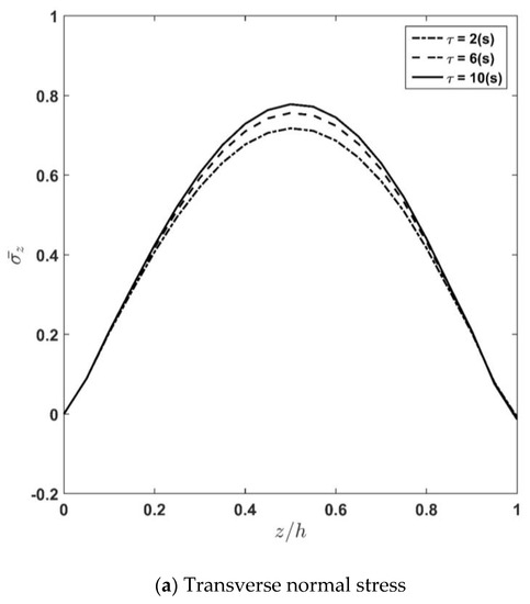
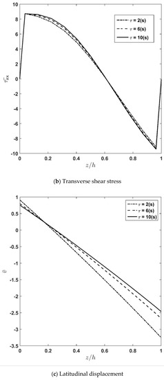
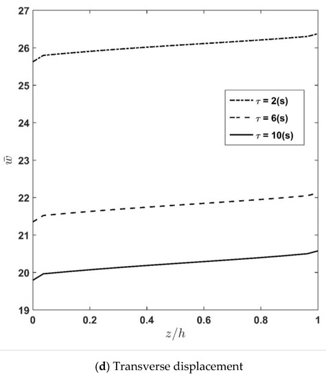
Figure 6. Effect of time constant variation, $\tau$, on the transverse normal and shear stresses, as well as latitudinal displacement and transverse displacements.

The time history of the stress and displacement components for different relaxation time constants $\tau$ is depicted in Figure 7a–c. The figures show that stress and displacement increase with time regardless of the value of $\tau$ and finally converge to their steady-state constant values. Moreover, it is seen that for all quantities for which their time history is depicted in this presentation, the rate of convergence to the ultimate values decreases when the time constant increases. From Figure 7c, it is seen that the influence of the relaxation time constant,$\tau$, on the deflection is more significant compared to other quantities.

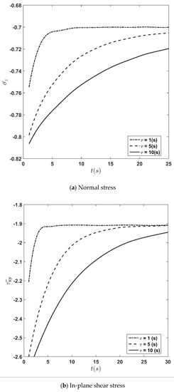
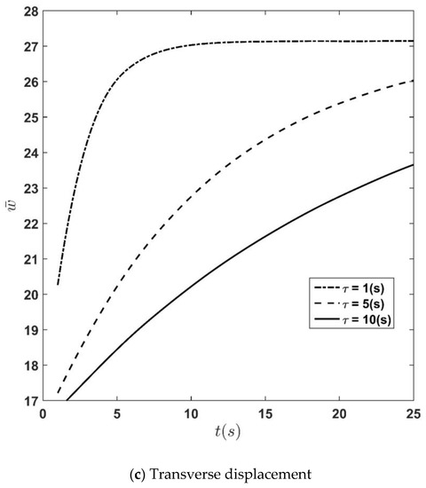
Figure 7. Time history of transverse normal stress, in-plane shear stress, and transverse displacement at the height of $\frac{\left(h_p+h_f+h_p\right)}{2}$ for different time constants.

Figure 8a–c demonstrate the effect of the applied voltage,$\hspace{0.17em}{\overline{\mathrm{V}}}_0$, on the variation of stresses and displacement along the thickness direction. According to the figures, increasing the voltage causes stresses and deflections to be increased. Moreover, it is seen that the effect of the applied voltage near the outer region of the FGM layer is more significant, which is due to the effect of the actuator layer. From Figure 8a it is observed that the normal longitudinal stress, ${\overline{\sigma }}_x$, is discontinuous at two interfaces due to the different elastic constants at the interfaces. Additionally, it is concluded that by moving from the lower surface to the top surface of the sandwich plate, the sign of this stress changes from tension to compression. Moreover, one can say that the maximum value of the normal longitudinal stress ${\overline{\sigma }}_x$ has a linear-like relation with the intensity of the applied voltage. To clarify this matter, it can be mentioned that the difference between the value of ${\overline{\sigma }}_x$ at the interface between the core and the upper piezoelectric face-layer computed at $\hspace{0.17em}{\overline{\mathrm{V}}}_0$ = 0 and ${\overline{\mathrm{V}}}_0$ = 0.01 is almost equal to the difference between the mentioned stress computed at ${\overline{\mathrm{V}}}_0$ = 0.01 and ${\overline{\mathrm{V}}}_0$ = 0.02. As Figure 8b shows, the continuity of transverse shear stress ${\overline{\tau }}_{zx}$ at the interfaces as well as at the top and bottom surfaces are satisfied, and its variation at the bottom surface is almost negligible. Figure 8c indicates that the slope for $\overline{\mathrm{w}}$ is almost independent of the ${\overline{\mathrm{V}}}_0$ value, but an increase in the applied voltage causes the plate to experience an increase in deflection. Moreover, it is observed that the slope of the deflection curve for the actuator layer increases when the applied voltage increases.

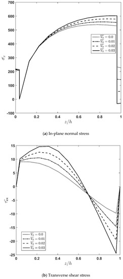
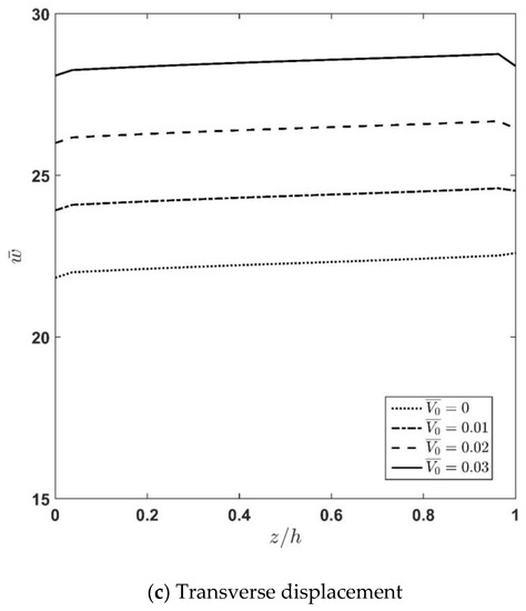
Figure 8. Influence of applied voltage variation of longitudinal normal stress, transverse shear stress, and transverse displacement along the thickness direction.

5. Conclusions

This article is dedicated to the analysis of the thermoviscoelastic response of the sandwich plate with a viscoelastic core and two surrounding piezoelectric face-layers simultaneously exposed to electro-thermal loading. The formulation is based on the 3D elasticity theory. The obtained equations were solved analytically using the state-space Fourier series method. It is noted that the governing equations before solving were converted to the Laplace domain and after solving the results were converted to the time domain by using an inverse Laplace transform. Our numerical results are summarized as the following list of conclusions:

• Increasing the length-to-thickness ratio $a/h$ leads to decrease in deflections and increase in stresses.
• In the absence of an applied voltage when $h/h_p\ge 150$, the effect of the piezoelectric layer thickness on the thermo-elastic behavior becomes negligible.
• Stiffness of the plate decreases by increasing $T_o$ and, accordingly, stresses and the deflection decrease.
• The effect of a temperature difference in the lower region is more significant than in the upper region due to the thermal barrier behavior of the FGM core at the upper surface.
• Increasing the relaxation time constant causes the stiffness of the viscoelastic plate and, accordingly, stress components to increase and the displacement to decrease.
• Increasing the relaxation time constant causes the rate of convergence to the elastic behaviour to decrease.
• The effect of the applied voltage near the outer region of the FGM layer is more significant due to the actuator layer’s effect.
• Deflection $\overline{\mathrm{w}}$ of the plate increases by increasing the applied voltage.
• Through-thickness distribution of deflection is linear in piezoelectric and FGM layers with different slope.
• Increasing the time constant $\tau$ causes delay in the steady state condition for stresses and displacement.
• Increasing the time constant $\tau$ causes a decrease in the transverse displacement $\overline{\mathrm{w}}$.
• The maximum values of transverse normal stress ${\overline{\sigma }}_z$ are not at the mid-thickness of the plate, which is due to the FGM property.

References

- Jagtap, K.R.; Lal, A.; Singh, B.N. Stochastic nonlinear bending response of functionally graded material plate with random system properties in thermal environment. Int. J. Mech. Mater. Des. 2012, 8, 149–167. [Google Scholar] [CrossRef]
- Alibeigloo, A.; Emtehani, A. Static and free vibration analyses of carbon nanotube-reinforced composite plate using differential quadrature method. Meccanica 2015, 50, 61–76. [Google Scholar] [CrossRef]
- Alibeigloo, A. Three-dimensional thermoelasticity analysis of graphene platelets reinforced cylindrical panel. Eur. J. Mech. A/Solids 2020, 81, 103941. [Google Scholar] [CrossRef]
- Phung-Van, P.; Thai, C.H.; Abdel-Wahab, M.; Nguyen-Xuan, H. Optimal design of FG sandwich nanoplates using size-dependent isogeometric analysis. Mech. Mater. 2019, 142, 103277. [Google Scholar] [CrossRef]
- Beg, M.S.; Yasin, M.Y. Bending, free and forced vibration of functionally graded deep curved beams in thermal environment using an efficient layerwise theory. Mech. Mater. 2021, 159, 103919. [Google Scholar] [CrossRef]
- Wang, Y.; Feng, C.; Yang, J.; Zhou, D.; Liu, W. Static response of functionally graded graphene platelet–reinforced composite plate with dielectric property. J. Intell. Mater. Syst. Struct. 2020, 31, 2211–2228. [Google Scholar] [CrossRef]
- Brischetto, S.; Torre, R. 3D Stress Analysis of Multilayered Functionally Graded Plates and Shells under Moisture Conditions. Appl. Sci. 2022, 12, 512. [Google Scholar] [CrossRef]
- Amiri Delouei, A.; Emamian, A.; Karimnejad, S.; Sajjadi, H.; Jing, D. Two-dimensional analytical solution for temperature distribution in FG hollow spheres: General thermal boundary conditions. Int. Commun. Heat Mass Transf. 2020, 113, 104531. [Google Scholar] [CrossRef]
- Amiri Delouei, A.; Emamian, A.; Karimnejad, S.; Sajjadi, H. A closed-form solution for axisymmetric conduction in a finite functionally graded cylinder. Int. Commun. Heat Mass Transf. 2019, 108, 104280. [Google Scholar] [CrossRef]
- Khan, Y.; Akram, S.; Athar, M.; Saeed, K.; Muhammad, T.; Hussain, A.; Imran, M.; Alsulaimani, H.A. The Role of Double-Diffusion Convection and Induced Magnetic Field on Peristaltic Pumping of a Johnson–Segalman Nanofluid in a Non-Uniform Channel. Nanomaterials 2022, 12, 1051. [Google Scholar] [CrossRef]
- Saeed, K.; Akram, S.; Ahmad, A.; Athar, M.; Imran, M.; Muhammad, T. Impact of partial slip on double diffusion convection and inclined magnetic field on peristaltic wave of six-constant Jeffreys nanofluid along asymmetric channel. Eur. Phys. J. Plus 2022, 137, 364. [Google Scholar] [CrossRef]
- Akram, S.; Razia, A.; Umair, M.Y.; Abdulrazzaq, T.; Homod, R.Z. Double-diffusive convection on peristaltic flow of hyperbolic tangent nanofluid in non-uniform channel with induced magnetic field. Math. Methods Appl. Sci. 2022. [Google Scholar] [CrossRef]
- Akram, S.; Athar, M.; Saeed, K.; Imran, M.; Muhammad, T. Slip impact on double-diffusion convection of magneto-fourth-grade nanofluids with peristaltic propulsion through inclined asymmetric channel. J. Therm. Anal. Calorim. 2022, 147, 8933–8946. [Google Scholar] [CrossRef]
- Akram, S.; Athar, M.; Saeed, K.; Umair, M.Y. Nanomaterials effects on induced magnetic field and double-diffusivity convection on peristaltic transport of Prandtl nanofluids in inclined asymmetric channel. Nanomater. Nanotechnol. 2022, 12, 18479804211048630. [Google Scholar] [CrossRef]
- Akram, S.; Athar, M.; Saeed, K.; Razia, A. Impact of slip on nanomaterial peristaltic pumping of magneto-Williamson nanofluid in an asymmetric channel under double-diffusivity convection. Pramana 2022, 96, 1–13. [Google Scholar] [CrossRef]
- Alibeigloo, A. Thermoelasticity analysis of functionally graded beam with integrated surface piezoelectric layers. Compos. Struct. 2010, 92, 1535–1543. [Google Scholar] [CrossRef]
- Alibeigloo, A.; Chen, W.Q. Elasticity solution for an FGM cylindrical panel integrated with piezoelectric layers. Eur. J. Mech. A/Solids 2010, 29, 714–723. [Google Scholar] [CrossRef]
- Kiani, Y.; Rezaei, M.; Taheri, S.; Eslami, M.R. Thermo-electrical buckling of piezoelectric functionally graded material Timoshenko beams. Int. J. Mech. Mater. Des. 2011, 7, 185–197. [Google Scholar] [CrossRef]
- Brischetto, S.; Carrera, E. Static analysis of multilayered smart shells subjected to mechanical, thermal and electrical loads. Meccanica 2013, 48, 1263–1287. [Google Scholar] [CrossRef]
- Alibeigloo, A. Three-dimensional thermoelasticity solution of functionally graded carbon nanotube reinforced composite plate embedded in piezoelectric sensor and actuator layers. Compos. Struct. 2014, 118, 482–495. [Google Scholar] [CrossRef]
- Alibeigloo, A. Thermoelastic solution for static deformations of functionally graded cylindrical shell bonded to thin piezoelectric layers. Compos. Struct. 2011, 93, 961–972. [Google Scholar] [CrossRef]
- Feri, M.; Alibeigloo, A.; Zanoosi, A.A.P. Three dimensional static and free vibration analysis of cross-ply laminated plate bonded with piezoelectric layers using differential quadrature method. Meccanica 2016, 51, 921–937. [Google Scholar] [CrossRef]
- Kulikov, G.M.; Plotnikova, S.V. An analytical approach to three-dimensional coupled thermoelectroelastic analysis of functionally graded piezoelectric plates. J. Intell. Mater. Syst. Struct. 2017, 28, 435–450. [Google Scholar] [CrossRef]
- Heydarpour, Y.; Malekzadeh, P.; Dimitri, R.; Tornabene, F. Thermoelastic analysis of functionally graded cylindrical panels with piezoelectric layers. Appl. Sci. 2020, 10, 1397. [Google Scholar] [CrossRef]
- Moradi-Dastjerdi, R.; Behdinan, K. Thermo-electro-mechanical behavior of an advanced smart lightweight sandwich plate. Aerosp. Sci. Technol. 2020, 106, 106142. [Google Scholar] [CrossRef]
- Zeng, S.; Peng, Z.; Wang, K.; Wang, B.; Wu, J.; Luo, T. Nonlinear Analyses of Porous Functionally Graded Sandwich Piezoelectric Nano-Energy Harvesters under Compressive Axial Loading. Appl. Sci. 2021, 11, 11787. [Google Scholar] [CrossRef]
- Xiang, H.J.; Shi, Z.F. Static analysis for functionally graded piezoelectric actuators or sensors under a combined electro-thermal load. Eur. J. Mech. -A/Solids 2009, 28, 338–346. [Google Scholar] [CrossRef]
- Koutsawa, Y.; Haberman, M.R.; Daya, E.M.; Cherkaoui, M. Multiscale design of a rectangular sandwich plate with viscoelastic core and supported at extents by viscoelastic materials. Int. J. Mech. Mater. Des. 2009, 5, 29–44. [Google Scholar] [CrossRef]
- Cai, Y.; Sun, H. Thermo-viscoelastic analysis of three-dimensionally braided composites. Compos. Struct. 2013, 98, 47–52. [Google Scholar] [CrossRef]
- Norouzi, H.; Alibeigloo, A. Three dimensional static analysis of viscoelastic FGM cylindrical panel using state space differential quadrature method. Eur. J. Mech.-A/Solids 2017, 61, 254–266. [Google Scholar] [CrossRef]
- Malikan, M.; Dimitri, R.; Tornabene, F. Effect of sinusoidal corrugated geometries on the vibrational response of viscoelastic nanoplates. Appl. Sci. 2018, 8, 1432. [Google Scholar] [CrossRef]
- Yang, Z.; Wu, P.; Liu, W.; Fang, H. Analytical Solutions for Functionally Graded Sandwich Plates Bonded by Viscoelastic Interlayer Based on Kirchhoff Plate Theory. Int. J. Appl. Mech. 2020, 12, 2050062. [Google Scholar] [CrossRef]
- Liu, C.; Shi, Y. A thermo-viscoelastic analytical model for residual stresses and spring-in angles of multilayered thin-walled curved composite parts. Thin-Walled Struct. 2020, 152, 106758. [Google Scholar] [CrossRef]
- Chen, J.; Han, R.; Liu, D.; Zhang, W. Active Flutter Suppression and Aeroelastic Response of Functionally Graded Multilayer Graphene Nanoplatelet Reinforced Plates with Piezoelectric Patch. Appl. Sci. 2022, 12, 1244. [Google Scholar] [CrossRef]
- Hetnarski, R.B.; Eslami, M.R.; Gladwell, G. Thermal Stresses: Advanced Theory and Applications; Springer: Berlin/Heidelberg, Germany, 2009; Volume 41. [Google Scholar]
- Sadd, M.H. Elasticity: Theory, Applications, and Numerics; Academic Press: Cambridge, MA, USA, 2009; ISBN 0-08-092241-4. [Google Scholar]
- Li, C.; Guo, H.; Tian, X.; He, T. Generalized thermoviscoelastic analysis with fractional order strain in a thick viscoelastic plate of infinite extent. J. Therm. Stress. 2019, 42, 1051–1070. [Google Scholar] [CrossRef]
- Alibeigloo, A. Thermo-elasticity solution of functionally graded plates integrated with piezoelectric sensor and actuator layers. J. Therm. Stress. 2010, 33, 754–774. [Google Scholar] [CrossRef]
- Abate, J.; Whitt, W. Numerical inversion of Laplace transforms of probability distributions. ORSA J. Comput. 1995, 7, 36–43. [Google Scholar] [CrossRef]
- Norouzi, H.; Alibeigloo, A. Three-dimensional thermoviscoelastic analysis of a FGM cylindrical panel using state space differential quadrature method. J. Therm. Stress. 2018, 41, 383–398. [Google Scholar] [CrossRef]
- Brischetto, S.; Leetsch, R.; Carrera, E.; Wallmersperger, T.; Kröplin, B. Thermo-mechanical bending of functionally graded plates. J. Therm. Stress. 2008, 31, 286–308. [Google Scholar] [CrossRef]
- Reddy, J.; Cheng, Z.-Q. Three-dimensional thermomechanical deformations of functionally graded rectangular plates. Eur. J. Mech. -A/Solids 2001, 20, 841–855. [Google Scholar] [CrossRef]
Disclaimer/Publisher’s Note: The statements, opinions and data contained in all publications are solely those of the individual author(s) and contributor(s) and not of MDPI and/or the editor(s). MDPI and/or the editor(s) disclaim responsibility for any injury to people or property resulting from any ideas, methods, instructions or products referred to in the content. |
© 2022 by the authors. Licensee MDPI, Basel, Switzerland. This article is an open access article distributed under the terms and conditions of the Creative Commons Attribution (CC BY) license (https://creativecommons.org/licenses/by/4.0/).