GPU-Accelerated Infill Criterion for Multi-Objective Efficient Global Optimization Algorithm and Its Applications

Abstract

In this work, a novel multi-objective efficient global optimization (EGO) algorithm, namely GMOEGO, is presented by proposing an approach of available threads’ multi-objective infill criterion. The work applies the outstanding hypervolume-based expected improvement criterion to enhance the Pareto solutions in view of the accuracy and their distribution on the Pareto front, and the values of sophisticated hypervolume improvement (HVI) are technically approximated by counting the Monte Carlo sampling points under the modern GPU (graphics processing unit) architecture. As compared with traditional methods, such as slice-based hypervolume integration, the programing complexity of the present approach is greatly reduced due to such counting-like simple operations. That is, the calculation of the sophisticated HVI, which has proven to be the most time-consuming part with many objectives, can be light in programed implementation. Meanwhile, the time consumption of massive computing associated with such Monte Carlo-based HVI approximation (MCHVI) is greatly alleviated by parallelizing in the GPU. A set of mathematical function cases and a real engineering airfoil shape optimization problem that appeared in the literature are taken to validate the proposed approach. All the results show that, less time-consuming, up to around 13.734 times the speedup is achieved when appropriate Pareto solutions are captured.

1. Introduction

The efficient global optimization (EGO) algorithm, which was first proposed by Jones et al. [1] in 1998, has proved to be very efficient for dealing with expensive-to-evaluate optimizations [2,3,4,5]. Benefited from the fundamental concepts of the Kriging surrogate model and the expected improvement (EI) criterion, EGO can always capture a high-quality optimal solution with relatively less objective function evaluations (FEs) compared to other popular optimization algorithms, such as genetic algorithms (GAs) [6]. Because of this advantage, the corresponding theory has been applied to a variety of modern engineering applications [7,8,9,10,11]. One must notice that the original EI criterion is initially designed for single-objective optimization (SOO) problems and cannot be applied to more important multi-objective optimization (MOO) problems directly.

It is well known that real engineering optimization problems usually come up with not only one single objective but also a set of objectives, which usually conflict with each other. Motivated by the outstanding behaviors of the traditional EGO algorithm in dealing with SOO problems, different methods have been developed by modifying the EGO algorithm to be able to cope with MOO problems [12,13,14], particularly for expensive-to-evaluate problems. For instance, the method, namely ParEGO, was developed by Knowles [12] for coping with MOO problems. Different aggregate single-objectives are updated iteration by iteration using the augmented Tchebycheff functions with different random vectors to balance the multiple sub-objectives. A similar method called MOEA/D-EGO was later proposed by Liu et al. [14]. These methods, which are realized in a way of transforming the MOO problem into an SOO problem associated with any available single-objective EGO optimizers, do show promise in the test cases appearing in the literature mentioned. However, because of the usage of several probabilistic parameters of corresponding optimization problems, they are usually not easy to directly apply to real time-consuming engineering optimizations [15,16]. In addition, only one optimal solution captured as a result of the transformed SOO problem is mostly weight dependence.

An alternative to avoiding the shortages mentioned is to capture a set of solutions distributed at the Pareto front of the MOO problem. The main challenge in capturing the distribution of Pareto solutions is modifying the EI infill criterion of the EGO algorithm to be suitable for updating Pareto solutions efficiently. For example, Keane et al. [13] developed the Euclidean distance-based EI (EI-ELU) infill criterion by maximizing the minimum distance between the expected central point of probability distribution and the Pareto points. A more recent hypervolume indicator-based criterion, which was proposed by Zitzler and Thiele [17], is more of interest for MOO problems. In recent decades, many practical contributions have been made to hypervolume-based infill metrics, such as works in hypervolume indicator [17,18], hypervolume improvement [19], S-metric [2,20], lower confidence bound (LCB) [2,21], expected hypervolume improvement (EHVI) [18,22], truncated expected hypervolume improvement (TEHVI) [23], and modified expected hypervolume improvement (MEHVI) [24].

In general, the hypervolume-based metric has been reported to be an outstanding metric for improving accuracy and distribution on the Pareto front of the MOO problem [24,25]. However, the calculation of such metrics is still struggling with enhancing the accuracy of computed hypervolume and reducing the computational complexity implementation. In view of accuracy enhancement, several notable methods have been successfully developed for computing hypervolume, such as the LebMeasure method [21,26], Overmars, and Yap method [27], hypervolume by slicing objectives (HSO) method [28], IHSO method [29], HypE method [30], and box decomposition method [31]. These methods have shown their powerful potential in obtaining a more accurate hypervolume value; however, their implementations are usually hugely complex due to the irregular geometry of the nondominated region of the Pareto front, particularly for the unimaginable Pareto front caused by many objectives. Alternatively, a Monte Carlo-based method is proposed by Emmerich [2,18] to reduce the computational complexity of related implementation, but high computational costs are still required due to the fact that there are many repeated nondominated calculations related to the Monte Carlo-based calculations of hypervolume. It can be imagined that such situations will be even worse for many objectives involved in the MOO problem. This might be the reason that the Monte Carlo-based method has rarely been reported in real applications of MOO problems in recent years. In contrast, for calculating hypervolume involved in infill criteria, the Monte Carlo-based method, a kind of statistical method, is quite easy to program in implementation, which is more preferred for MOO applications by new users. Therefore, despite the low efficiency associated with calculations of hypervolume, the attractive programing simplicity of the Monte Carlo-based method still motivates the present research to find an efficient way to propose new treatments.

In the present work, an effort has been made to develop a novel approach for computing multi-objective infill criteria for efficient global optimization (EGO) algorithms. The work applies the outstanding hypervolume-based expected improvement metric to enhance Pareto solutions in view of their accuracies and distributions on the Pareto front, and the values of sophisticated hypervolume improvement (HVI) are technically approximated by counting the Monte Carlo sampling points under the modern GPU (graphics processing unit) architecture. The calculation of the sophisticated HVI, which has proven to be the most time-consuming part with many objectives, can be light in programed implementation due to such counting-like simple operations. Meanwhile, the time consuming of massive computing associated with such HVI approximation is greatly alleviated by parallelizing in the GPU. It can be learned from the test cases that significant speedups are achieved by the proposed GMOEGO algorithm.

The rest of the paper is organized as follows. The related works, including an overview of the traditional EGO algorithm and the hypervolume-based EI criterion, are described in Section 2. Then, in Section 3, the modified EGO-based multi-objective optimization method is presented by adopting the new proposed GPU-based Monte Carlo method. After presenting representative function tests in Section 4, a more practicable aerodynamic optimization case is further presented to investigate the efficiency of the proposed algorithm in Section 5. Finally, in Section 6, concluding remarks are drawn.

2. Related Works

2.1. Traditional Single-Objective EGO Algorithm

A study of EGO to be used for optimizations with multiple objectives. The traditional EGO algorithm is usually developed for optimization with a single objective. For the sake of completeness, a brief discussion of the traditional single-objective EGO algorithm [1] is presented in this section. To be the core components of the traditional EGO algorithm, the Kriging surrogate model and EI infill criterion ensure its high efficiency of EGO and global searching ability.

Kriging was first proposed by Krige [32] in 1951, and its formulation with $d$ variables and $n_s$ samples can be described as follows: let $n_s$ sampled points be $\mathit{X}{\mathit{s}}^{n_s}=\left\{{\mathbf{x}}^1,{\mathbf{x}}^2,\cdots ,{\mathbf{x}}^{n_s}\right\}$, and their associated objective function values are $\mathit{Y}{\mathit{s}}^{n_s}=\left\{{\mathbf{y}}^1,{\mathbf{y}}^2,\cdots ,{\mathbf{y}}^{n_s}\right\}$, in which the $i$-th sample point and its objective value are ${\mathbf{x}}^i=\left(x_1^i,x_2^i,\cdots ,x_d^i\right)$, ${\mathbf{y}}^i=\left(y_1^i,y_2^i,\cdots ,y_d^i\right)$, respectively, for $i=1, 2, \cdots , n_s$.

$$Y({\mathbf{x}}^i)={\displaystyle \sum _{j=1}^k{\beta }_j{f}_j({\mathbf{x}}^i)+z({\mathbf{x}}^i)}$$

(1)

where $f_j\left({\mathbf{x}}^i\right)$ are k known regression models, and ${\beta }_j$ are correlation coefficients of $f_j\left({\mathbf{x}}^i\right)$, $z({\mathbf{x}}^i)$ is a stochastic model and its mean is zero and variance is ${\delta }_z{}^2$. The covariance between two design points ${\mathbf{x}}^i$ and ${\mathbf{x}}^j$ can be written as

$$Cov\left[z\left({\mathbf{x}}^i\right), z\left({\mathbf{x}}^j\right)\right]={\delta }_z{}^2\mathit{R}\left[R\left({\mathbf{x}}^i, {\mathbf{x}}^j\right)\right]$$

(2)

where $i, j=1, 2, \cdots , n_s$; a symmetric matrix, $\mathit{R}$, is a correlation function that reflects the relationship between all the sample points; $R$ is a correlation function defined by the user, and a widely used form of $R$ can be expressed as [33]

$$R\left({\mathbf{x}}^i,{\mathbf{x}}^j\right)={\displaystyle \prod _{k=1}^{d}esp\left(-{\theta }_k{\left|x_k^i-x_k^j\right|}^{p_k}\right)}$$

(3)

where ${\theta }_k>0$, $0\le p_k\le 2$ are two hyper parameters. Once the hyper parameters ${\theta }_k$ and $p_k$ are determined, the prediction $\widehat{y}\left(\mathbf{x}\right)$ of $Y$ at the location $\mathbf{x}$ can be calculated by

$$\widehat{y}\left(\mathbf{x}\right)=\widehat{\beta }+{\mathit{r}}^T\left(\mathbf{x}\right){\mathit{R}}^{-1}\left(\mathbf{y}-\mathit{1}\beta \right)$$

(4)

in which the n-vector, $\mathit{r}\left(\mathbf{x}\right)$, reflects the correlations between the predicted location $\mathbf{x}$ and the sampled locations $\mathit{R}\left(\mathbf{x},{\mathbf{x}}^j\right)$, where $j=1, 2, \cdots , n_s$; $\mathit{1}$ is an n-vector of ones; and an n-vector, $\mathbf{y}$, is the value of accurate response; $\beta$ is the mean of $Y\left(\mathbf{x}\right)$, and $\widehat{\beta }$ denotes the generalized least squares estimator of $\beta$, which is defined as $\widehat{\beta }={\left({\mathit{1}}^T{\mathit{R}}^{-1}\mathit{1}\right)}^{-1}{\mathit{1}}^T{\mathit{R}}^{-1}\mathbf{y}$ [33], and then, the mean squared error (MSE) of $\widehat{y}\left(\mathbf{x}\right)$ can be written as

$$\mathrm{MSE}\left[\widehat{y}\left(\mathbf{x}\right)\right]={\delta }_Z{}^2\left(1-{\mathit{r}}^T\left(\mathbf{x}\right){\mathit{R}}^{-1}\mathit{r}\left(\mathbf{x}\right)\right)$$

(5)

The hyper parameter ${\theta }_k$ (see Equation (3)) can be determined by using the maximum likelihood estimation (MLE) approach with the limitation of ${\theta }_k>0$

$$\mathrm{Ln}\left(\mathrm{Likelihood}\right)=-\frac{1}{2}\left(n \ln \left({\delta }_z{}^2\right)+\ln \left|\mathit{R}\right|\right)$$

(6)

where ${\delta }_z{}^2={\left(\mathbf{y}-\mathit{1}\widehat{\beta }\right)}^T{\mathit{R}}^{-1}\left(\mathbf{y}-1\widehat{\beta }\right)/n$, and by solving Equation (6), the Kriging model can be constructed. The approximation $\widehat{y}\left(\mathbf{x}\right)$ and MSE can be obtained by Equations (4) and (5).

Once a Kriging surrogate model is constructed, the EI function (Equation (7)) can be determined using a specific optimizer. Assume the $\widehat{y}\left(\mathbf{x}\right)$ follows the normal distribution $Y~N\left(\mu , s^2\right)$, where $\mu$ is the Kriging predictor $\widehat{y}\left(\mathbf{x}\right)$ defined in Equation (4), $s^2\left(\mathbf{x}\right)$ is the MSE (see Equation (5)), and $y_{\min }$ is the minimum of all the sample points. Then the EI function at location $\mathbf{x}$ can be expressed as follows [1]

$$E\left[I\left(\mathbf{x}\right)\right]=\{\begin{array}{cc}\left(y_{\min }-\widehat{y}\left(\mathbf{x}\right)\right)\Phi \left(\frac{y_{\min }-\widehat{y}\left(\mathbf{x}\right)}{s\left(\mathbf{x}\right)}\right)+s\left(\mathit{x}\right)\varphi \left(\frac{y_{\min }-\widehat{y}\left(\mathbf{x}\right)}{s\left(\mathbf{x}\right)}\right)& s\left(\mathbf{x}\right)>0\\ 0& s\left(\mathbf{x}\right)=0\end{array}$$

(7)

where $\Phi$ and $\varphi$ are the normal cumulative distribution function and the normal probability density function, respectively. This criterion is considered a balance of “exploration and exploitation”.

It should be pointed out that the EI criterion is initially designed for SOO problems, and cannot be directly applied to MOO problems. That is, for MOO problems, the new EI criterion should be constructed for the multi-objective EGO algorithm, which will be discussed in the next section.

2.2. EHVI Infill Criterion for the Multi-Objective EGO Algorithm

As discussed in Section 1, one of the most popular criteria designed for a multi-objective EGO (MOEGO) algorithm is the EHVI criterion, which is modified from HVI. Therefore, the HVI is described here before presenting the EHVI criterion.

Considering the MOO problem with $m>1$ objective functions $f_m$: $\mathbf{\chi } \mapsto {\mathbf{ℝ}}^m$, the MOO problem can be briefly expressed as

$$\begin{array}{l}\underset{\mathbf{x}\in \mathbf{\chi }}{\mathrm{Minmize}}\mathbf{y}=\left\{f_1\left(\mathbf{x}\right), f_2\left(\mathbf{x}\right), \dots , f_m\left(\mathbf{x}\right)\right\}\\ \mathrm{Subject} \mathrm{to} \mathbf{x}\in \left[\mathit{l}, \mathit{u}\right]\end{array}\}$$

(8)

where $\mathbf{\chi }\subseteq {\mathbf{ℝ}}^d$, $\mathbf{y}\in 𝒀\subseteq {\mathbf{ℝ}}^m$. $\mathit{l}$ and $\mathit{u}$ are the lower and upper constraints, respectively, of the design variable vector $\mathbf{x}$. $d$ denotes the number of design variables, and $m$ is the number of objectives.

Assume the problem (8) to be optimized iteration by iteration with the EGO optimizer and take the set of Pareto front solutions (points) at the n-th iteration of problem (8) as ${𝒫}_n=\left\{{\mathbf{y}}_1,{\mathbf{y}}_2,\cdots ,{\mathbf{y}}_{n_{dom}}\right\}$, where $n_{dom}$ is the number of current Pareto front points; all the elements in ${𝒫}_n$ are nondominated by each other, and can be mathematically expressed as

$$\forall i, j\in \left\{1, 2, \cdots , n_{dom}\right\}\wedge \left(i\ne j\right):\left({\mathbf{y}}_i\nprec {\mathbf{y}}_j\right)\wedge \left({\mathbf{y}}_j\nprec {\mathbf{y}}_i\right)$$

in which $a\nprec b$ means $a$ does not dominate $b$, and on the contrary, $a\prec b$ means $a$ dominates $b$. ${\mathbf{y}}_i=\left\{y_i^1,y_i^2,\cdots ,y_i^m\right\}$ denotes the coordinate of the i-th point in ${𝒫}_n$.

In order to compute the hypervolume used in the EHVI criterion, a reference point $ℛ=\left\{r_1,r_2,\cdots , r_m\right\}\in {\mathbf{ℝ}}^m$ is usually required to be defined by designers before the calculation, and then the hypervolume of the current Pareto front related to the reference point, $\mathscr{H}\left({𝒫}_n, ℛ\right)$, can be expressed as

$$\mathscr{H}\left({𝒫}_n, ℛ\right)={\displaystyle {\int }_{\left(\exists {\mathbf{y}}_i\in {𝒫}_n\right)\prec \mathbf{y}\prec ℛ}\mathrm{d}\mathbf{y}}$$

(9)

In Equation (9), one must notice that the hypervolume is equivalent to the region, which is dominated by at least one point of ${𝒫}_n$ and itself dominates the reference point, as shown in Figure 1, shaded with blue oblique lines.

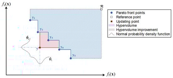
Figure 1. Example of a hypervolume indicator with two objectives.

Assume that the current predicted updating point is ${\mathbf{y}}^{\prime }$, the HVI indicator $I_{\mathscr{H}}\left({\mathbf{y}}^{\prime }, {𝒫}_n\right)$ of the red area in Figure 1 can then be defined as:

$$I_{\mathscr{H}}\left({\mathbf{y}}^{\prime }, {𝒫}_n\right)=\{\begin{array}{cc}\mathscr{H}\left(\left({𝒫}_n\cup \left\{{\mathbf{y}}^{\prime }\right\}\right), ℛ\right) - \mathscr{H}\left({𝒫}_n, ℛ\right)& \nexists {\mathbf{y}}_i\in {𝒫}_n: {\mathbf{y}}_i\prec {\mathbf{y}}^{\prime }\\ 0& \mathrm{Otherwise}\end{array}$$

(10)

It can be noted that only when ${\mathbf{y}}^{\prime }$ falls in the ${𝒫}_n$ nondominated region can the positive value of HVI be obtained. As expected, a large value of HVI reflects an improvement in the Pareto front solutions. Hence, the HVI, $I_{\mathscr{H}}\left({\mathbf{y}}^{\prime }, {𝒫}_n\right)$, can be taken as the infill criterion directly, and its further enhanced criterion of the HVI indicator, namely $E{I}_{\mathscr{H}}\left(\mathbf{x}\right)$ of EHVI indicator, is proposed by Emmerich et al. [2] and could be predicted by the expected improvement function $E\left[I_{\mathscr{H}}\right]$, which reads

$$E{I}_{\mathscr{H}}\left(\mathbf{x}\right)=E\left[I_{\mathscr{H}}\right]={\displaystyle {\int }_{{\mathbf{y}}^{\prime }\in \Omega }{I}_{\mathscr{H}}\left({\mathbf{y}}^{\prime }, {𝒫}_n\right)\mathrm{PDF}\left({\mathbf{y}}^{\prime }\right)d{\mathbf{y}}^{\prime }}$$

(11)

where the nondominated region $\Omega$ of the current Pareto front is defined as

$$\Omega =\left\{\mathbf{y}\in {\mathfrak{ℝ}}^m|\left(\mathbf{y}\prec ℛ\right)\wedge \left(\nexists {\mathbf{y}}_i\in {𝒫}_n: {\mathbf{y}}_i\prec \mathbf{y}\right)\right\}$$

(12)

$\mathrm{PDF}\left({\mathbf{y}}^{\prime }\right)$ is the probability density function, which can be estimated by

$$\mathrm{PDF}\left({\mathbf{y}}^{\prime }\left(\mathbf{x}\right)\right)=\{\begin{array}{cc}{\displaystyle {\prod }_{i=1}^m\varphi \left(\frac{{y^{\prime }}_i-{\widehat{y}}_i\left(\mathbf{x}\right)}{s_i\left(\mathbf{x}\right)}\right)}& s_i\left(\mathbf{x}\right)>0\\ 1& s_i\left(\mathbf{x}\right)=0\end{array}$$

(13)

It can be learned that the enhancement of the EHVI criterion is realized by considering the uncertainty of the prediction with the probability density function (see ${\varphi }_1$ and ${\varphi }_2$ in Figure 1), which could balance the exploration and exploitation. Unfortunately, there is a lack of direct calculating formula of both the HVI and EHVI criteria due to the fact that the shape of the Pareto front usually appears to be extremely irregular, as illustrated in Figure 2. This results in the calculation of the HVI or EHVI criteria appearing to be of current interest and usually requiring sophisticated programing steps with high time-consuming for both implementation and computation [30,34]. In order to have an improvement, an alternative Monte Carlo-based approach with GPU acceleration is proposed in the present work for computing these infill criteria, which will be mainly addressed in the next section.

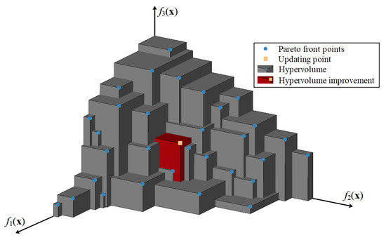
Figure 2. Example of geometry shape of hypervolume and its improvement.

3. Novel Approach to Computing Infill Criteria for MOEGO

A novel approach to calculating the hypervolume-based infill criterion for the MOEGO algorithm is developed here by coupling with the Monte Carlo approach. In order to make it clear, in Section 3.1, the main concepts of the Monte Carlo approach are briefly described. In Section 3.2, the GPU-accelerated infill criterion is constructed for the MOEGO algorithm, and in Section 3.3, the resulting framework of the MOEGO algorithm is discussed theoretically.

3.1. A Brief Description of the Monte Carlo Approach

For the sake of easy implementation, the Monte Carlo approach is considered to calculate the HVI or EHVI in the present work. According to the principle of the theory [35], the HVI (see Figure 1 and Equation (10)) could be calculated via the hit-or-miss method (also called the rejection method) [36]. The basic structure of the Monte Carlo-based HVI (MCHVI) is presented for obtaining the HVI, as shown in Algorithm 1.

Algorithm 1. MCHVI algorithm

In order to make it clear, Monte Carlo sampling points and approximation of the MCHVI indicator are illustrated with two objectives as shown in Figure 3. In the present work, the value of the MCHVI indicator is approximated by counting the number $n_q$ of the sampling points located in the domain of dependence (red area in Figure 3) by

$$I_{\mathscr{H}}\left({\mathbf{y}}^{\prime }, {𝒫}_n\right)\approx \raisebox{1ex}{$n_q$}\!\left/ \!\raisebox{-1ex}{$n_p$}\right.\times V$$

(14)

where $n_p$ is the number of Monte Carlo sampling points (see line 3 of Algorithm 1), and $V$ is the volume of the hypercube. Such counting-like simple operations are light in programed implementation, and it can be imagined that the value of the MCHVI indicator is proportional to the size of the Monte Carlo sampling points. However, in order to avoid misguidance caused by the approximate MCHVI indicator, the number of Monte Carlo sapling points is preferred to be as large as possible, which in turn requires massive arithmetic operations associated with predicting the value of the MCHVI indicator will be required. This situation could be alleviated through GPU accelerating, which will be mainly considered and addressed in Section 3.2.

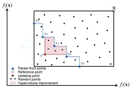
Figure 3. Example of HVI calculation by the Monte Carlo-based method with two objectives.

Once the value of HVI indicator $I_{\mathscr{H}}$ is obtained, the value of EHVI indicator $E{I}_{\mathscr{H}}$ can be approximated by the generalized form of the Monte Carlo estimator [37], which can be expressed as

$$E{I}_{\mathscr{H}}\left(\mathbf{x}\right)\approx \frac{1}{N}{\displaystyle \sum _{i=1}^N{I}_{\mathscr{H}}\left({\mathbf{y}}^{mc}{}_i, {𝒫}_n\right)}$$

(15)

where $\left\{{\mathbf{y}}_1^{mc}, {\mathbf{y}}_2^{mc},\cdots ,{\mathbf{y}}_N^{mc}\right\}$ are the $N$ random samples of the Gaussian distribution with mean $\widehat{y}$ and standard deviation $s$. The number $N$ is a user-defined parameter, and in this paper, following the work of [38], a fixed number of 1000 is used for all test cases presented in Section 4. The $I_{\mathscr{H}}\left({\mathbf{y}}^{mc}{}_i, {𝒫}_n\right)$ is predicted by the MCHVI algorithm (see Algorithm 1), which is the main time-consuming part of the EHVI indicator. and hence will be implemented in GPU architecture, as discussed in the next section.

3.2. GPU-Accelerated Infill Criterion for the MOEGO Algorithm

In this section, GPU implementation is presented for computing the value of the MCHVI indicator. As described in Algorithm 1, a mass of independent arithmetic operations associated with the dominated or non-dominated identifications (see Algorithm 1, line 6) are proved to be time-consuming. Fortunately, such tasks are mostly weak-dependent compute-intensive and are very suitable for GPU parallel architecture [39,40,41]. Therefore, such a kind of computation is implemented on the GPU to achieve acceleration. In order to obtain a global view of our implementation, the corresponding general framework of the program is given in Figure 4. It should be noted that necessary computing data, including the coordinates of all Monte Carlo sample points, Pareto front points, and updating points, are designed to be prepared on the CPU side and then sent to the GPU side before starting the GPU calculations. After all the calculations of the GPU side are finished, the total number of sample points that satisfy the definition of the MCHVI indicator is fetched (see Algorithm 1, line 6), and then sent back to the CPU side for the MCHVI estimation. That is, only time-consuming and suitable tasks are implemented on the GPU.

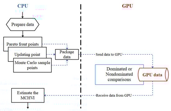
Figure 4. General framework of GPU-based MCHVI indicator value calculations.

Algorithm 2 presents the key code snippet of the GPU subroutine for MCHVI calculations, in which MCSP_d is the number of Monte Carlo sample points, Front_d denotes the Pareto front, and HV_d is the computed MCHVI number nq (see lines 7 and 8 in Algo-rithm 1). The corresponding thread hierarchy is designed as shown in Figure 5. It can be learned that a GPU thread is assigned to the calculations related to each Monte Carlo sample point. All GPU threads are organized into a queue of thread blocks inside a thread grid to be adjusted to the double-layer structure of GPU hardware [42]. In the corresponding code snippet (Algorithm 2), the thread index is first calculated using three build-in parameters, $blockdim$, $blockIdx$ and $threadIdx$ (for details, see [42]). After the thread index is obtained, the locations of each Monte Carlo sample point (with the same thread index) are then compared with the existing Pareto front and current updating points. If the Monte Carlo point is located in the dominated region, an integer of 1 is added to the value of the MCHVI indicator using a build-in function of $atomicadd$ (see line 8 in Algorithm 2).

Algorithm 2. Code snippet of the kernel for GPU-based MCHVI calculation

1 attributes(global) subroutine kernel_MCHV(MCSP_d, Front_d, HV_d) 2  i = (blockIdx%x-1)*blockDim%x + threadIdx%x !thread Index 3  4  do j = 1, nFront !loop over all Pareto front points and updating point 5   if(isInvalid(MCSP_d(:,i),Front_d(:,j)) return !judge of domination 6  end do 7  8  istat = atomicadd(HV_d, 1)  !accumulate result to global memory 9 end subroutine

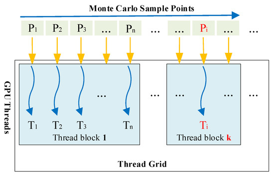
Figure 5. Thread hierarchy designed for GPU-based MCHVI indicator.

While the corresponding CPU subroutine for calling the GPU subroutine (Algorithm 2) is presented in Algorithm 3, in which MCSP is the number of Monte Carlo sample points, Front de-notes the Pareto front, and HV is the computed MCHVI number nq (See lines 7 and 8 in Algorithm 1).in which the parameters of thread hierarchy, including number of threads per thread block and total number of thread blocks, are assigned in a specific build-in symbol of “<<<·>>>”. Following our previous GPU works [40,41], a suggested value of 64 is assigned as the number of threads per block; hence, the total number of thread blocks is equal to $ceiling\left(n_p,64\right)$, a rounding function to return the least integer greater than or equal to its argument, in which $n_p$ is the total number of Monte Carlo sample points. The efficiency of the MOO problem could be expected to improve due to the GPU accelerated implementation, which will be addressed in the following sections.

Algorithm 3. Code snippet of the CPU subroutine for calling $kernel\_MCHV$

1 subroutine calKernel_MCHV(MCSP, Front, HV) 2  NTPB = 64 !Number of threads per block 3  NBPG = ceiling(MCSP/64) ! Number of blocks per grid 4  5  MCSP_d = MCSP; Front_d = Front !Copy data to GPU 7  8  call kernel_MCHV <<<NBPG,NTPB>>> (MCSP_d,Front_d,HV_d) !call the kernel 9  10   HV = HV_d !Send result back to CPU 11 end subroutine

3.3. Multi-Objective EGO Method with Modified Infill Criterion

The resulting GPU accelerated Monte Carlo-based multi-objective EGO algorithm, namely GMOEGO, can be summarized as Algorithm 4, as follows.

Algorithm 4. GMOEGO Algorithm
Step 1	Initialization: Use the DOE method to generate a set of sample points $\mathit{X}{\mathit{s}}^{n_s}$ within design space, and evaluate their objective values $\mathit{Y}{\mathit{s}}^{n_s}$ of $\mathit{X}{\mathit{s}}^{n_s}$ (for definition of $n_s$, see Section 2.1).
Step 2	Updating Model: Construct $m$ Kriging surrogate models based on current sample points $\left(\mathit{X}{\mathit{s}}^{n_s},\mathit{Y}{\mathit{s}}^{n_s}\right)$ for each objective.
Step 3	Nondominated sort: Sort the current sample points $\left(\mathit{X}{\mathit{s}}^{n_s},\mathit{Y}{\mathit{s}}^{n_s}\right)$ by nondominated strategy to obtain the current set of Pareto front point ${𝒫}_n$.
Step 4	Searching for Optimal Updating Point: Based on the Kriging models constructed, search for the optimal updating location by maximizing the EHVI indicator (Equation (11)) based on the Kriging models constructed, in which the indicator is calculated based on the Monte Carlo approach on a GPU computational platform.
Step 5	Objective Function Evaluation: Calculate the values of objective functions at the optimal updating location obtained in Step 4 to update the sample values to obtain $\left(\mathit{X}{\mathit{s}}_{}^{n_s+1},\mathit{Y}{\mathit{s}}_{}^{n_s+1}\right)$.
Step 6	Stopping criterion: Check the stopping criterion. If satisfied, output the optimized Pareto front points and stop; if not, go back to Step 2.

In the present work, we use the Latin Hypercube Sampling (LHS) [43] is selected as the DOE method (see step 1) for its space filling properties. A global genetic algorithm (GA) is selected to be used in constructing Kriging surrogate models (see step 2) and searching the optimal updating location (in step 4) for the objectives of them are both functions (see Equations (6) and (15)), which are easy for GA optimizers; for details about GA, we refer to [6]. The stopping criterion in step 6 is limited by the maximum number of FEs.

The algorithm presented has been programed to be different modules with Fortran language. The performance of the algorithm presented will be demonstrated and analyzed through comparison with the traditional EGO algorithm, which will be mainly addressed in the next section.

4. Numerical Tests and Analysis

In order to have a view of performance, seven representative mathematical functions with different properties appeared in the literature [16,38,44] are carefully selected to validate the present algorithm. For the sake of convenience, the definitions of the selected functions are listed in the Appendix A.

All the tests are carried out on a personal computer with the Intel Core i9-9900k CPU (8 cores) and GTX-1066 GPU. The code is developed in CUDA Fortran, and the operating system is Windows 10. The first function (ZDT1) is used in Section 4.1 to investigate the speedup effect of the number of Monte Carlo sample points. In Section 4.2, all test functions are then used to validate the present GMOEGO algorithm in comparison with the optimizers listed in Table 1. In the following sections, the size of the initial EGO sample points is set as $n_s=6\times d-1$, and all optimizations are carried out under the limited maximum number of FEs. In the present work, $n_{FEs}\le 200$ is assigned to be the stop criterion used in step 6 of Algorithm 4. The speedup ratio SUR of the total computation cost between the two algorithms is defined as

$$SUR=\frac{T_{GMOEGO}}{T_{MOEGO}}$$

(16)

where $T_{MOEGO}$ is the total computational cost of the reference MOEGO algorithm, which is parallelized on the platform of Intel Core i9-9900k CPU with 8 cores, and $T_{GMOEGO}$ is the total computational cost of the present GMOEGO algorithm, which is run on the GTX-1066 GPU platform.

Table 1. Test results of the speedup ratio of ZDT1.

Number of Monte Carlo Sample Points	Algorithm	Total Cost (Hours)	MCHVI Cost (Hours)	SUR of Total Cost (Times)
$1\times {10}^2$	MOEGO	0.239	0.001	0.916
	GMOEGO	0.261	0.018
$1\times {10}^3$	MOEGO	0.253	0.010	0.920
	GMOEGO	0.275	0.032
$1\times {10}^4$	MOEGO	0.403	0.169	1.404
	GMOEGO	0.287	0.051
$1\times {10}^5$	MOEGO	2.146	1.893	5.896
	GMOEGO	0.364	0.124
$1\times {10}^6$	MOEGO	28.081	27.830	12.575
	GMOEGO	2.233	1.986

In order to assess the performance of the GMOEGO algorithm, the Inverted Generational Distance (IGD) metric [45] is used in the numerical tests in this section. The IGD metric can be mathematically expressed as

$$\mathrm{IGD}\left(P^{*},P\right)=\frac{{\displaystyle {\sum }_{\nu \in P^{*}}d\left(\nu ,P\right)}}{\left|P^{*}\right|}$$

(17)

in which $P^{*}$ is usually a set of $n$ points uniformly distributed on the theoretical Pareto front, while $P$ is the optimized Pareto front. $d\left(\nu ,P\right)$ is the minimum Euclidean distance between $\nu$ and the points in $P$, and $\left|P^{*}\right|$ represents the number of points in $P^{*}$. It can be seen that a low value of $\mathrm{IGD}\left(P^{*},P\right)$, means the optimized $P$ is very close to the theoretical Pareto front $P^{*}$. This is desired by designers.

4.1. Analysis of GPU Speedup Effect

As mentioned above, the computational cost of the MCHVI calculation on the CPU is very time consuming (the most consuming part). In order to investigate the speedup effect of the number of Monte Carlo sample points, the GMOEGO algorithm with different amounts of Monte Carlo sample points, $1\times {10}^2$, $1\times {10}^3$, $1\times {10}^4$, $1\times {10}^5$, and $1\times {10}^6$, is validated, and the traditional MOEGO algorithm is taken as the reference optimizer for comparison. For the purpose of saving testing time, one test function, the ZDT1 function with 2 variables (d = 2), is selected for analyzing the performance of GPU implementation.

The test results for the speedup ratio of ZDT1 are listed in Table 1. It can be learned that the most time-consuming part, up to 99 percent of the overall costs (the MOEGO algorithm with $1\times {10}^6$ Monte Carlo sample points), are really spent in MCHVI calculations (see the fourth column of Table 1), the time consuming of GMOEGO presented are now speedup by proposed GPU implementation, and significant acceleration, up to 12.575 speedup ratio, are achieved (see the last column in Table 1). In order to make it clear, the corresponding speedup ratio of the total cost to a different number of Monte Carlo sample points is illustrated in Figure 6. When the Monte Carlo sample points are few, it fails to have GPU speedup (see Figure 6) due to the fact that the cost of data exchange between the CPU and GPU side is mainly dominated in such circumstances, as listed in Table 1. It can also be observed that a continual increase in speedups related to the growing number of sample points can be achieved, which are favorable for coping with the problems in the case of a large number of sample points required. Such situations usually occur in complex MOO problems under the requirement of high accuracy in capturing the Pareto front.

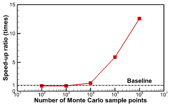
Figure 6. Speedup ratio of total cost to different numbers of Monte Carlo sample points.

4.2. Numerical Tests of the GMOEGO Algorithm

In order to investigate the performance of the proposed GMOEGO algorithm, all six test functions (see Appendix A) are selected as the test functions. In order to mimic real engineering optimizations, test functions with more variables are constructed: 10 variables for ZDT1-ZDT3 functions, 5 variables for DTLZ2 function, 8 variables for DTLZ5 function, and 10 variables for DTLZ7. In contrast, these test cases are also optimized by the referenced MOEGO algorithm, which is run on a 12-core CPU (Intel Core i9-9900k) in parallel. The Monte Carlo sample points of the GMOEGO algorithm are set as $n_p=1\times {10}^5$ for two-objective functions (ZDT1-ZDT3), and $n_p=1\times {10}^6$ for three-objective functions (DTLZ2, DTLZ 5, and DTLZ7). Both algorithms are performed on the same computational platform mentioned at the beginning of this section.

The test results are shown in Table 2. The Pareto solution distributions compared with the theoretical true Pareto front are illustrated in Figure 7. It can be noticed that, for all the test cases, the Pareto solution distributions obtained by the GMOEGO algorithm and the referenced MOEGO algorithm are very close to the theoretical true Pareto front, and the obtained IGD values listed in the third column of Table 2 are around ${10}^{-3}$ to ${10}^{-5}$, which indicates the optimized Pareto fronts are very close to the theoretical Pareto fronts.

Table 2. Results of the test functions.

Test Function	Algorithm	IGD	Total Cost (Hours)	MCHVI Cost (Hours)	SUR of Total Cost (Times)
ZDT1	MOEGO	$1.817\times {10}^{-5}$	4.952	4.511	5.246
	GMOEGO	$2.080\times {10}^{-5}$	0.944	0.703
ZDT2	MOEGO	$2.124\times {10}^{-5}$	5.247	4.530	6.559
	GMOEGO	$3.878\times {10}^{-5}$	0.800	0.601
ZDT3	MOEGO	$1.594\times {10}^{-4}$	4.249	2.474	4.634
	GMOEGO	$1.216\times {10}^{-4}$	0.917	0.636
DTLZ2	MOEGO	$3.200\times {10}^{-3}$	32.943	32.843	13.734
	GMOEGO	$3.070\times {10}^{-3}$	2.397	2.365
DTLZ5	MOEGO	$1.260\times {10}^{-4}$	28.014	26.138	11.906
	GMOEGO	$1.290\times {10}^{-4}$	2.353	2.272
DTLZ7	MOEGO	$5.530\times {10}^{-3}$	29.679	27.426	12.408
	GMOEGO	$3.740\times {10}^{-3}$	2.392	2.183

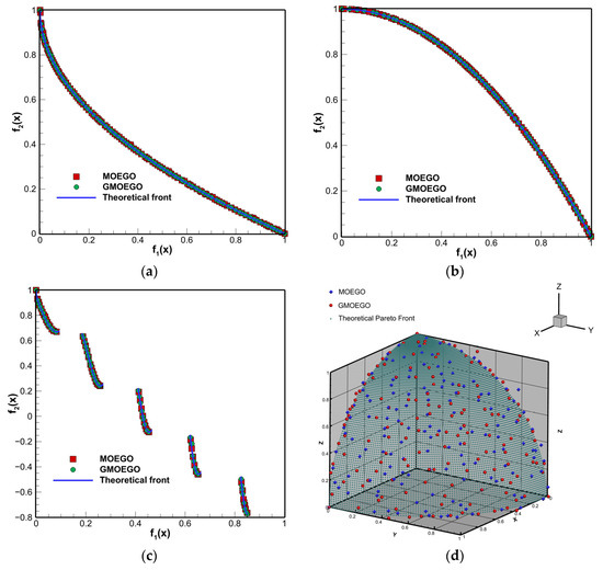
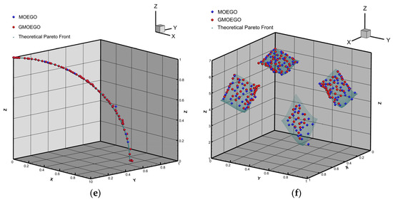
Figure 7. Pareto front comparisons: (a) ZTD1; (b) ZTD2; (c) ZTD3; (d) DTLZ2; (e) DTLZ5; (f) DTLZ7.

The total wall-clock time costs and the MCHVI calculation costs are given in the fourth and fifth columns of Table 2, and their corresponding comparison histories are illustrated in Figure 8. It can be seen that, as analyzed in Section 3, the computational cost of the MCHVI calculations is the main part of the overall optimization procedure, and it is not hard to imagine that improving this module of the optimization algorithm will bring the most benefits, and as expected, the computational cost improvements of the proposed GMOEGO algorithm mainly come from the speedup of the MCHVI calculations. The speedup ratio of the GMOEGO in comparison with the MOEGO algorithm is given in the sixth column of Table 2. It can be seen that benefit from the GPU implementation, speedups up to 13.734 times are achieved in comparison with the cost of the MOEGO algorithm based on 8 cores in parallel, which shows the effectiveness of the GPU architecture.

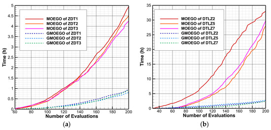
Figure 8. Wall-clock time history comparisons: (a) ZDT series functions; (b) DTLZ series functions.

5. Aerodynamic Design Optimization

In order to investigate the performance of the proposed GMOEGO algorithm in real engineering optimization applications, an aerodynamic airfoil shape optimization case [46] is selected to test the algorithm. The baseline of the airfoil is RAE2822 under the conditions of $Ma=0.75$, $Re=6.5\times {10}^6$, and $\alpha ={2.31}^{\circ }$. The optimization target is to maximize the lift-drag ratios under two different Mach numbers: $Ma=0.6$, $Ma=0.75$. The optimization problem can be defined as:

$$\begin{array}{l}\begin{array}{cc}Max.& {\left(C_L/C_D\right)}_{Ma=0.6}\\ & {\left(C_L/C_D\right)}_{Ma=0.75}\end{array}\}\\ s.t.\hspace{1em}\left\{x_i\in \mathit{X}|i=1, 2, \cdots , n\right\}\end{array}$$

(18)

in which $C_L$ is the lift coefficient, $C_D$ is the drag coefficient, $\mathit{X}$ is the design parameters of the Hicks–Henne parametrization method [47], and $n$ is the number of control parameters. In this paper, $n=14$ is set to parametrize the airfoil geometry.

The Computational Fluid Dynamics (CFD) simulator used to calculate the aerodynamic coefficients is the open-source software SU2 [48]. In this work, the Jameson scheme is selected as the spatial discretization scheme, and the Spalart-Allmaras (SA) one equation turbulence model is used for turbulence closure. The computational O-type mesh of RAE2822 airfoil is shown in Figure 9.

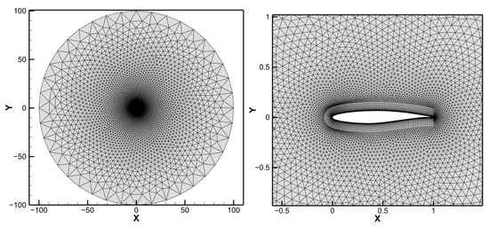
Figure 9. Computational mesh of RAE2822.

During the optimizations, 43 initial samples are set by using the LHS method, and the maximum FEs of CFD evaluations is limited to 400. The computations are carried out on the computational platform of Intel Core i9-9900k CPU (8 cores) with GTX-1066 GPU. After 400 CFD evaluations, the Pareto front obtained by the proposed GMOEGO algorithm is illustrated in Figure 10. Three representative optimized solutions marked with Optimum 1–3 in Figure 10 are selected to show their aerodynamic performances.

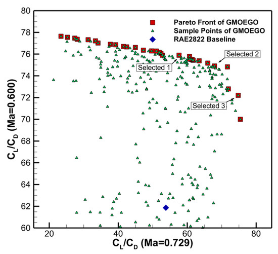
Figure 10. Optimization results of the GMOEGO algorithm.

The comparison of aerodynamic performance between the baseline and the selected optimized airfoils is listed in Table 3. It can be seen in the table that for optimum 1, the lift-drag ratio is increased by 7.14% for objective 1 and 22.57% for objective 2 when compared to the baseline. For optimum 2, the optimized ratios are 26.26% and 21.10%, respectively. For optimum 3, the lift-drag ratio of objective 1 is increased to 39.04%, and objective 2′s improvement of lift-drag ratio is 16.73%.

Table 3. Comparison of aerodynamic performance between baseline and optimized airfoils.

Airfoil	Number of Objective	${\mathit{C}}_{\mathit{L}}/{\mathit{C}}_{\mathit{D}}$
Baseline	1	53.81
	2	61.86
Optimum 1	1	57.65 (+7.14%)
	2	75.90 (+22.57%)
Optimum 2	1	67.94 (+26.26%)
	2	74.91 (+21.10%)
Optimum 3	1	74.82 (+39.04%)
	2	72.21 (+16.73%)

The geometry shape of the optimized airfoil and the baseline are compared in Figure 11. Figure 12 illustrates the comparison of $C_p$ distributions of two objectives, and the corresponding $C_p$ comparisons are depicted in Figure 13. It can be learned that for objective 1, the shock wave of optimum 3 is weaker than that of optimums 1 and 2, which results in a significantly increasing lift-drag ratio (39.04%). For objective 2, the increase in lift-drag ratios is mainly due to the increase in lift coefficients. It can also be seen that different points on the Pareto front relate to the different aerodynamic performances of airfoils. Designers can select a specific airfoil depending on specific application scenarios and requirements.

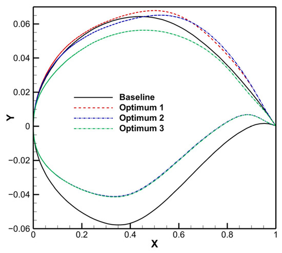
Figure 11. Comparison of shape between optimized airfoil and baseline.

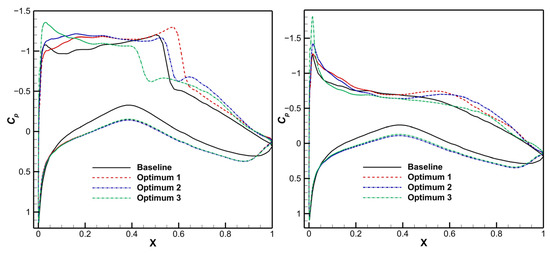
Figure 12. Comparison of pressure coefficient distribution between optimized airfoil and baseline.

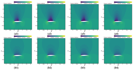
Figure 13. Contour of pressure coefficient comparison between optimized airfoil and baseline: (a1) Baseline of objective 1; (a2) Optimum 1 of objective 1; (a3) Optimum 2 of objective 1; (a4) Optimum 3 of objective 1; (b1) Baseline of objective 2; (b2) Optimum 1 of objective 2; (b3) Optimum 2 of objective 2; (b4) Optimum 3 of objective 2.

Furthermore, in order to investigate the acceleration effect of the proposed GMOEGO algorithm in real applications, the aerodynamic airfoil shape optimization case above is also optimized by the counterpart referenced MOEGO algorithm. The computational platform is Intel Core i9-9900k CPU (8 cores), and all the other setups remain the same, as mentioned at the beginning of this section.

The optimized Pareto fronts obtained by MOEGO and GMOEGO algorithms for comparison is in Figure 14. It can be seen that both algorithms could obtain similar Pareto fronts. Figure 15 shows the comparison of the wall-clock time histories of the two algorithms, and the corresponding comparison results are listed in Table 4. The comparison shows that, benefiting from the Monte Carlo-based GPU-acceleration technique, a significantly speedup ratio, up to 7.27 times, is achieved. The fourth column of Table 4 shows the wall-clock time cost of MCHVI, and the corresponding histories are also depicted in Figure 15. It can be seen that the MCHVI calculation is the most time-consuming part of the whole optimization procedure of both algorithms, and the acceleration of the GMOEGO algorithm is mainly driven by the acceleration of this MCHVI calculation part. The significant speedup ratio shows the capability of the proposed GMOEGO algorithm to deal with real engineering optimizations.

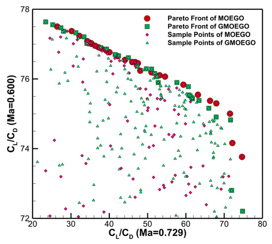
Figure 14. Obtained optimal Pareto fronts.

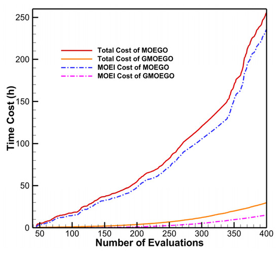
Figure 15. Time cost histories.

Table 4. Speedup results of MOEGO and GMOEGO algorithms.

Algorithm	Platform	Total Cost (Hours)	MCHVI Cost (Hours)	SUR of Total Cost (Times)
MOEGO	Intel Core i9-9900k CPU (with 8 cores in parallel)	255.78	235.69	7.27
GMOEGO	GTX-1066	35.20	17.13

6. Conclusions

In this paper, the GMOEGO algorithm has been successfully developed for MOO problems. The outstanding hypervolume-based EI criterion is adopted as the multi-objective infill criterion computed in a novel Monte Carlo-based way of high efficiency. The time consumption of massive computing associated with Monte Carlo-based HVI approximation (MCHVI) is greatly alleviated by parallelizing in the GPU. The algorithm presented has been successfully validated by a set of typical mathematical test functions. Positive speedups up to 13.734 times can be achieved when compared with the traditional Monte Carlo-based MOEGO algorithm. The presented algorithm has also been successfully applied to an aerodynamic optimization problem, and a 7.27-times speedup is achieved with limited expensive-to-evaluate CFD evaluations, which shows the potential capability of the algorithm to deal with real engineering MOO problems in view of accuracy and efficiency.

References

- Jones, D.R.; Schonlau, M.; Welch, W.J. Efficient Global Optimization of Expensive Black-Box Functions. J. Glob. Optim. 1998, 13, 455–492. [Google Scholar] [CrossRef]
- Emmerich, M.T.M.; Giannakoglou, K.C.; Naujoks, B. Single- and multiobjective evolutionary optimization assisted by Gaussian random field metamodels. IEEE Trans. Evol. Comput. 2006, 10, 421–439. [Google Scholar] [CrossRef]
- Forrester, A.I.J.; Keane, A.J. Recent advances in surrogate-based optimization. Prog. Aerosp. Sci. 2009, 45, 50–79. [Google Scholar] [CrossRef]
- Deng, F.; Qin, N.; Liu, X.; Yu, X.; Zhao, N. Shock control bump optimization for a low sweep supercritical wing. Sci. China Technol. Sci. 2013, 56, 2385–2390. [Google Scholar] [CrossRef]
- Xu, S.; Chen, H. Nash game based efficient global optimization for large-scale design problems. J. Glob. Optim. 2018, 71, 361–381. [Google Scholar] [CrossRef]
- Whitley, D. A genetic algorithm tutorial. Stat. Comput. 1994, 4, 65–85. [Google Scholar] [CrossRef]
- Sóbester, A.; Leary, S.J.; Keane, A.J. On the Design of Optimization Strategies Based on Global Response Surface Approximation Models. J. Glob. Optim. 2005, 33, 31–59. [Google Scholar] [CrossRef]
- Horowitz, B.; Guimarães, L.J.d.N.; Dantas, V.; Afonso, S.M.B. A concurrent efficient global optimization algorithm applied to polymer injection strategies. J. Pet. Sci. Eng. 2010, 71, 195–204. [Google Scholar] [CrossRef]
- Han, Z.-H.; Görtz, S.; Zimmermann, R. Improving variable-fidelity surrogate modeling via gradient-enhanced Kriging and a generalized hybrid bridge function. Aerosp. Sci. Technol. 2013, 25, 177–189. [Google Scholar] [CrossRef]
- Chung, I.-B.; Park, D.; Choi, D.-H. Surrogate-based global optimization using an adaptive switching infill sampling criterion for expensive black-box functions. Struct. Multidiscip. Optim. 2018, 57, 1443–1459. [Google Scholar] [CrossRef]
- Xu, S.; Chen, H.; Zhang, J. A study of Nash-EGO algorithm for aerodynamic shape design optimizations. Struct. Multidiscip. Optim. 2019, 59, 1241–1254. [Google Scholar] [CrossRef]
- Knowles, J. ParEGO A hybrid algorithm with on-line landscape approximation for expensive multiobjective optimization problems. IEEE Trans. Evol. Comput. 2006, 10, 50–66. [Google Scholar] [CrossRef]
- Keane, A.J. Statistical Improvement Criteria for Use in Multiobjective Design Optimization. AIAA J. 2006, 44, 879–891. [Google Scholar] [CrossRef]
- Liu, W.; Zhang, Q.; Tsang, E.; Liu, C.; Virginas, B. On the Performance of Metamodel Assisted MOEA/D. In ISICA 2007: Advances in Computation and Intelligence; International Symposium on Intelligence Computation and Applications; Kang, L., Liu, Y., Zeng, S., Eds.; Springer: Berlin/Heidelberg, Germany, 2007; Volume 4683, pp. 547–557. [Google Scholar]
- Namura, N.; Shimoyama, K.; Obayashi, S. Expected Improvement of Penalty-Based Boundary Intersection for Expensive Multiobjective Optimization. IEEE Trans. Evol. Comput. 2017, 21, 898–913. [Google Scholar] [CrossRef]
- Qingfu, Z.; Wudong, L.; Tsang, E.; Virginas, B. Expensive Multiobjective Optimization by MOEA/D With Gaussian Process Model. IEEE Trans. Evol. Comput. 2010, 14, 456–474. [Google Scholar] [CrossRef]
- Zitzler, E.; Thiele, L. Multiobjective optimization using evolutionary algorithms—A comparative case study. In Parallel Problem Solving from Nature—PPSN V; Lecture Notes in Computer Science; Eiben, A.E., Bäck, T., Schoenauer, M., Schwefel, H.-P., Eds.; Springer: Berlin/Heidelberg, Germany, 1998; Volume 1498, pp. 292–301. [Google Scholar]
- Emmerich, M.T.M. Single- and Multi-objective Evolutionary Design Optimization Assisted by Gaussian Random Field Metamodels. Ph.D. Thesis, University of Dortmund, Dortmund, Germany, 2005. [Google Scholar]
- Emmerich, M.; Beume, N.; Naujoks, B. An EMO Algorithm Using the Hypervolume Measure as Selection Criterion. In The Third International Conference on Evolutionary Multi-Criterion Optimization, Berlin, Heidelberg; Evolutionary Multi-Criterion Optimization; Springer: Berlin/Heidelberg, Germany, 2005; pp. 62–76. [Google Scholar]
- Ponweiser, W.; Wagner, T.; Biermann, D.; Vincze, M. Multiobjective Optimization on a Limited Budget of Evaluations Using Model-Assisted S-Metric Selection. In Parallel Problem Solving from Nature—PPSN X; Springer: Berlin/Heidelberg, Germany, 2008; pp. 784–794. [Google Scholar]
- Fleischer, M. The Measure of Pareto Optima Applications to Multi-objective Metaheuristics. In Evolutionary Multi-Criterion Optimization; Springer: Berlin/Heidelberg, Germany, 2003; pp. 519–533. [Google Scholar]
- Wagner, T.; Emmerich, M.; Deutz, A.; Ponweiser, W. On Expected-Improvement Criteria for Model-based Multi-objective Optimization. In Parallel Problem Solving from Nature, PPSN XI; Springer: Berlin/Heidelberg, Germany, 2010; pp. 718–727. [Google Scholar]
- Yang, K.; Deutz, A.H.; Yang, Z.; Back, T.; Emmerich, M. Truncated expected hypervolume improvement: Exact computation and application. In Congress on Evolutionary Computation; Springer: Berlin/Heidelberg, Germany, 2016; pp. 4350–4357. [Google Scholar]
- Li, Z.; Wang, X.; Ruan, S.; Li, Z.; Shen, C.; Zeng, Y. A modified hypervolume based expected improvement for multi-objective efficient global optimization method. Struct. Multidiscip. Optim. 2018, 58, 1961–1979. [Google Scholar] [CrossRef]
- Yang, K.; Emmerich, M.; Deutz, A.; Bäck, T. Multi-Objective Bayesian Global Optimization using expected hypervolume improvement gradient. Swarm Evol. Comput. 2019, 44, 945–956. [Google Scholar] [CrossRef]
- Zitzler, E. Evolutionary Algorithms for Multiobjective Optimization Methods and Applications. Ph.D. Thesis, Swiss Federal Institute of Technology, Zürich, Switzerland, 1999. [Google Scholar]
- Beume, N.; Rudolph, G. Faster S-Metric Calculation by Considering Dominated Hypervolume as Klee’s Measure Problem. In Proceedings of the Second IASTED International Conference on Computational Intelligence, San Francisco, CA, USA, 20–22 November 2006; pp. 233–238. [Google Scholar]
- While, L.; Hingston, P.; Barone, L.; Huband, S. A Faster Algorithm for Calculating Hypervolume. IEEE Trans. Evol. Comput. Optim. Appl. 2006, 10, 29–38. [Google Scholar] [CrossRef]
- Bradstreet, L.; While, L.; Barone, L. A Fast Incremental Hypervolume Algorithm. IEEE Trans. Evol. Comput. 2008, 12, 714–723. [Google Scholar] [CrossRef][Green Version]
- Bader, J.; Zitzler, E. HypE An algorithm for fast hypervolume-based many-objective optimization. Evol. Comput. 2011, 19, 45–76. [Google Scholar] [CrossRef]
- Yang, K.; Emmerich, M.; Deutz, A.; Bäck, T. Efficient Computation of Expected Hypervolume Improvement Using Box Decomposition Algorithms. J. Glob. Optim. 2019, 75, 3–34. [Google Scholar] [CrossRef]
- Krige, D.G. A statistical approach to some basic mine valuation problems on the Witwatersrand. J. South Afr. Inst. Min. Metall. 1951, 52, 119–139. [Google Scholar]
- Sekishiro, M.; Venter, G.; Balabanov, V. Combined Kriging and Gradient-Based Optimization Method. In Proceedings of the 11th AIAA/ISSMO Multidisciplinary Analysis and Optimization Conference, Portsmouth, VA, USA, 6–8 September 2006; p. AIAA 2006-7091. [Google Scholar]
- Jiang, S.; Zhang, J.; Ong, Y.S.; Zhang, A.N.; Tan, P.S. A Simple and Fast Hypervolume Indicator-Based Multiobjective Evolutionary Algorithm. IEEE Trans. Cybern. 2015, 45, 2202–2213. [Google Scholar] [CrossRef] [PubMed]
- Hammersley, J.M.; Handscomb, D.C.; Weiss, G. Monte Carlo Methods. Phys. Today 1965, 18, 55. [Google Scholar] [CrossRef]
- Evans, M.; Swartz, T. Approximating Integrals via Monte Carlo and Deterministic Methods; OUP Oxford: Oxford, UK, 2000. [Google Scholar]
- Luo, C.; Shimoyama, K.; Obayashi, S. Kriging Model Based Many-Objective Optimization with Efficient Calculation of Expected Hypervolume Improvement. In Proceedings of the 2014 IEEE Congress on Evolutionary Computation (CEC), Beijing, China, 6–11 July 2014. [Google Scholar]
- Feng, D. Research on Efficient Global Optimization Algorithm and Its Application. Ph.D. Thesis, Nanjing University of Aeronautics and Astronautics, Nanjing, China, 2011. [Google Scholar]
- Ma, Z.; Wang, H.; Pu, S. GPU computing of compressible flow problems by a meshless method with space-filling curves. J. Comput. Phys. 2014, 263, 113–135. [Google Scholar] [CrossRef]
- Zhang, J.; Chen, H.; Cao, C. A graphics processing unit-accelerated meshless method for two-dimensional compressible flows. Eng. Appl. Comput. Fluid Mech. 2017, 11, 526–543. [Google Scholar] [CrossRef]
- Zhang, J.-L.; Ma, Z.-H.; Chen, H.-Q.; Cao, C. A GPU-accelerated implicit meshless method for compressible flows. J. Comput. Phys. 2018, 360, 39–56. [Google Scholar] [CrossRef]
- NVIDIA. CUDA C++ Programming Guide, Version 10. 2010. Available online: https://docs.nvidia.com/cuda/cuda-c-programming-guide/index.html (accessed on 8 September 2022).
- Kenny, Q.Y.; Li, W.; Sudjianto, A. Algorithmic construction of optimal symmetric Latin hypercube designs. J. Stat. Plan. Inference 2000, 90, 145–159. [Google Scholar]
- Deb, K.; Thiele, L.; Laumanns, M.; Zitzler, E. Scalable Test Problems for Evolutionary Multi-Objective Optimization. In Evolutionary Multiobjective Optimization. Advanced Information and Knowledge Processing; Abraham, A., Jain, L., Goldberg, R., Eds.; Springer: London, UK, 2005. [Google Scholar]
- Zhang, Q.; Li, H. MOEA/D: A multiobjective evolutionary algorithm based on decomposition. IEEE Trans. Evol. Comput. 2007, 11, 712–731. [Google Scholar] [CrossRef]
- Zhang, X.S.; Liu, J.; Luo, S.B. An improved multi-objective cuckoo search algorithm for airfoil aerodynamic shape optimization design. Hangkong Xuebao/Acta Aeronaut. Et Astronaut. Sinica 2018, 40, 5. [Google Scholar]
- Hicks, R.M.; Henne, P.A. Wing design by numerical optimization. J. Aircr. 1978, 15, 407–412. [Google Scholar] [CrossRef]
- Economon, T.D.; Palacios, F.; Copeland, S.R.; Lukaczyk, T.W.; Alonso, J.J. SU2: An open-source suite for multiphysics simulation and design. AIAA J. 2016, 54, 828–846. [Google Scholar] [CrossRef]
Disclaimer/Publisher’s Note: The statements, opinions and data contained in all publications are solely those of the individual author(s) and contributor(s) and not of MDPI and/or the editor(s). MDPI and/or the editor(s) disclaim responsibility for any injury to people or property resulting from any ideas, methods, instructions or products referred to in the content. |
© 2022 by the authors. Licensee MDPI, Basel, Switzerland. This article is an open access article distributed under the terms and conditions of the Creative Commons Attribution (CC BY) license (https://creativecommons.org/licenses/by/4.0/).