2. Materials & Methods
The complete model building process in useeior v1.0.0 requires the following six successful steps and returns a model object as the primary output:
For hybrid models, hybridization processes such as aggregation and/or disaggregation of sectors are incorporated in step 2 and 3.
To simplify the model building process, the six steps are integrated into a wrapper function,
buildModel, that builds a USEEIO model in one line of code, and provides logging of the build process using the
logging package [
21]:
model <- buildModel(modelname)
Before building a model, it is recommended to check if the model is available in useeior using this function:
seeAvailableModels()
useeior v1.0.0 comes with nine built-in national models (
Table 1), and their configuration files are found in the ‘inst/extdata/modelspecs/’ folder.
Model configurations are stored in relevant .yml (interchangeable with .yaml) files. YAML is a simple text-based format used to store configuration data across the USEEIO tool ecosystem [
11].
useeior uses the
configr package [
22] to parse YAML files.
2.1. Model Initialization
The first step in the model building process is to initialize the model according to the input model name, and paths to configuration files if provided. This step establishes the scope, e.g., single-region or two-region, and focus, e.g., specific or all environmental impacts, of the model.
model <- initializeModel(modelname, configpaths)
If the desired model is available in useeior, it is initialized based on modelname only, i.e., configpaths = NULL. This loads the built-in model configuration .yml file with that model name, and related aggregation/disaggregation configuration, and .yml and data .csv files.
Alternatively, a user-customized model can be initialized as long as its configuration files, including model and related hybridization configuration (in .yml format only), as well as data files (in .csv format only), are prepared following the format of configuration and data files of the available models. All configuration and data files must be accessible in the user directory specified in model configuration, i.e., configpaths = user_directory.
Model initialization returns a model object in list form that contains two elements: model specs and crosswalk. Specs stored the model specifications sourced directly from the model configuration files include:
Basic information including the name of the model, model region acronym, model type, and pointers to hybridization, such as aggregation and disaggregation;
Basic IO specifications including base IO schema, base IO level, IO year, model region acronym, IO data source, base price type, base with redefinitions or not, commodity or industry type, and scrap included or not;
Satellite table specifications including the name of environmental satellite tables, years represented by flows included in the satellite table, path of the source file, source category used for sectors in the satellite table, year and level of resolution of the sectors, original flow source, function name for additional processing of the satellite table, and metadata of satellite table;
Indicator specifications including name, code, group, and unit of indicator, path of the source file, function name and parameters for additional processing of the indicator, and metadata of indicator; and
Demand vectors specifications including a pointer to default demand vectors (i.e., a production vector, a consumption vector, and domestic version of the two vectors), and optional demand vectors, such as household purchase that contains name, type, year, system, and location information.
The crosswalk is a sector correspondence table of five columns for sets of BEA and NAICS codes, and any custom codes used in the current model:
NAICS—2- to 6-digit NAICS codes (7–10 digit codes exist for manufacturing and mining industries);
BEA_Sector—code used at the BEA sector level;
BEA_Summary—code used at the BEA summary level
BEA_Detail—code used at the BEA detail level;
USEEIO—code used at the model level of detail, including any adjustments for hybridization.
The crosswalk is a fundamental table in the
useeior model building process, as it connects the BEA and NAICS classification systems, which have notably different commodity and industry sectors, and enables mapping from one system to the other. An example of the crosswalk is presented in
Table S1 in the Supplementary Information (SI). In
useeior v1.0.0, the crosswalk is built based on 2012 BEA and NAICS codes, with an inclusion of 2007 NAICS codes, according to the 2012 to 2007 NAICS concordance by Census Bureau [
23]. The correspondences between BEA and NAICS codes were adopted from the BEA–NAICS relationship table, published in national IO accounts by BEA [
20], which presents a hierarchy of the BEA codes at sector, summary, and detail levels, as well as how each level relates to the NAICS code structure. Two adjustments were applied to the original BEA–NAICS table in order to create a crosswalk that captured all correspondences between BEA and NAICS sectors:
With a complete crosswalk, useeior successfully and seamlessly harmonizes economic and environmental data that are categorized by BEA, NAICS, and original classifications.
2.2. Economic Input–Output Data
In
useeior, the most recent IO data are the form of “Make” (showing the production of commodities by industries) and “Use” (showing the consumption of commodities by industries and by final demand) tables compiled by BEA [
20], saved in native R data formats, .rda, via automated downloading and writing functions. These tables are available at three levels of sector resolution: “Detail” (405 commodities by 405 industries), “Summary” (73 commodities by 71 industries), and “Sector” (17 commodities by 15 industries).
The summary and sector levels tables are released annually by BEA, while the detailed tables are produced roughly every five years, with 2012 representing the most recent release [
20]. Therefore, in
useeior v1.0.0, the summary and sector make and use tables are available for years 2010–2018, while the detail tables are only available for the year 2012.
The Make and Use tables compiled by BEA were available “before redefinition” and “after redefinition”. Redefinition adjusts secondary products “from the industry that produced it to the industry in which it is primary”. [
25] In
useeior, “before redefinition” tables are used, as they are more aligned with the majority of environmental data that reflect the original industry activities that occurred [
1].
Additionally, the use tables are available in producer price and purchaser price. Existing model configuration files in
useeior used the use tables in producer price.
useeior provides the option to convert the model from producer to purchaser price, with additions of trade and transportation margins [
26].
In EEIO modeling, the direct requirements matrix
and domestic direct requirements matrix
can be derived from the Make and Use tables to build EEIO models in two forms: industry-by-industry or commodity-by-commodity.
useeior is capable of building industry (industry-by-industry) and commodity (commodity-by-commodity) models. The former was the most suitable for EEIO models, with a focus on industries and environmental impacts from related producing processes; the latter was most relevant for EEIO models concerned with products and services and their associated materials. A direct requirements matrix derived based on two distinct assumptions, industry–technology and commodity–technology, yields different results. The former assumes that all commodities produced by the same industry have the same input structure, while the latter assumes that each commodity has a unique input structure, regardless of the industry that produced it [
25].
useeior v1.0.0 implements the industry–technology model.
Other economic data, including multi-year economic gross output, gross output chained price index, the margins table, and the import matrix, are also prepared and made available for immediate use in useeior.
Model IO data are loaded upon model initialization and with paths to configuration files if provided.
model <- loadIOData(model, configpaths)
After this step, the model object is expanded to include core IO data and related metadata for building the desired model, including:
The Make table in industry-by-commodity form;
Use and domestic use tables split into intermediate consumption, final demand, and value added in commodity-by-industry and commodity-by-component forms (note: domestic use table = use table − import matrix);
Commodity and industry output in model year, as well as in a range of multiple years in commodity-by-year and industry-by-year forms;
A Margins in commodity-by-margin-sector form disclosing producer price, trade (retail and wholesale) + transportation cost, and purchaser price of each commodity, used for converting from producer price to purchaser price, and vice versa;
Metadata of the IO data-code, name and group details about commodity, industry, final demand component, value added component, and margin sector;
IO data and metadata of hybridization if pointers to hybridization, such as aggregation and disaggregation, were not NULL in model specifications.
It is during this step of the model building process that custom hybridization of the model object occurs, when specified in the model configuration file. Currently, useeior only supports hybridization in the form of model aggregation and disaggregation, though support for other forms of hybridization is in progress. For model aggregation, the user only needs to input one additional .yml file to specify which sectors are to be aggregated. For model disaggregation, several additional input files need to be provided:
A .yml file containing a list of sectors, including the sector to be disaggregated and the new sectors that will take its place;
Two .csv files for the Use and Make tables (one for each) that specify the allocation values from the original to the disaggregated sectors. If the user does not have the data available to provide the allocation values, both .csv files can be omitted and the disaggregation proceeds uniformly based on the number of sectors specified;
A .csv file providing inputs for disaggregation of the satellite tables (see next section).
For all aggregation and disaggregation procedures, the commodity and industry sums are compared for equality across the Use and Make tables to ensure that the economic balance is maintained. If user inputs result in an unbalanced model, useeior attempts to balance the tables using a RAS approach. If this balancing is unsuccessful, the program execution halts and requests revised input files that will result in a balanced model.
2.3. Environmental Data and Satellite Tables
useeior characterizes the amount of environmental releases/losses, resource use, waste generation, and employment by model-specified industry, through the use of national totals of flows by NAICS industry and the crosswalk created in
Section 2.1. National totals of flows by NAICS industry data used in
useeior can be generated by a Python-based tool called FLOWSA [
15], which structures data in a flow-by-sector (FBS) format. The latest version of FLOWSA, v1.0.1, delivers FBS data that covers a variety of flow types, including criteria and hazardous air emissions, point source industrial releases to water and soil, use of land, use of water, and employment. To support impact assessment and a consistent flow naming system across data sources, flows in FLOWSA conform to the Federal Elementary Flow List (FEDEFL) [
27]. The FBS data to build the models specified in
useeior v1.0.0 are retrieved from the EPA Data Commons [
28] via automated functions in
useeior.
These flow-by-NAICS-industry data are transformed into flow-by-model-sector format, and loaded as satellite tables via the NAICS-to-BEA crosswalk. Value added by BEA industry are also considered flow data, but are directly loaded from the IO data that was added in the previous step.
model <- loadandbuildSatelliteTables(model)
A Satellite Tables component is added in the model object after this step. In the new component, the satellite tables are stored in totals_by_sector, while flow metadata were stored in flows. Each type of flow had a designated satellite table. Following the loading of all satellite tables, useeior identified instances of flows reported by the same sector from multiple satellite tables as a means to avoid double counting. All satellite tables were formatted into a standard structure that included the following columns:
Flow name, context, universally unique identifier (UUID), amount, unit, location, and data year;
Sector code and name;
Data quality scores for data reliability, temporal correlation, geographical correlation, technological correlation, and data collection.
Flow metadata displays unique flows found across all satellite tables with names, contexts, UUIDs, and units were sourced from FEDEFL.
Satellite, or totals_by_sector, tables provide a full picture of flows from and to the environment. They are used to calculate impact coefficients and validate the model.
If aggregation or disaggregation is specified during model build, each satellite table is aggregated or disaggregated upon loading. Specifications for disaggregating environmental data can be provided in one of two ways. If flow totals are provided for a given flow for any of the new sectors,
useeior replaces the existing satellite table data for that flow with the data in the
supplementary disaggregation file. Alternatively, flow ratios can be provided for one or more flows in a satellite table. If the FlowRatio field was supplied,
useeior disaggregates each flow to the new sectors according to the supplied ratios. In either case, if data for a specific flow are not provided,
useeior disaggregates the existing satellite table data for that flow proportional to gross industry output of the new sectors.
2.4. Indicators and Life Cycle Impact Assessment Characterization Factors
Model indicators quantitatively aggregate the environmental flow data to their corresponding impact categories, through the use of life cycle impact assessment (LCIA) characterization factors. For example, flows of greenhouse gases are valued as carbon dioxide equivalencies. To support the use of environmental flow data retrieved from FLOWSA, standard LCIA characterization factors generated by the LCIA formatter were used to populate model indicators [
16]. Users can choose from a number of available methods in the LCIA formatter including the Tool for Reduction and Assessment of Chemicals and Other Impacts (TRACI) [
29], ReCiPe [
30], etc., to generate LCIA factors that suit their needs. For any model, the method parameter is customizable and can be modified under the indicators section in model specifications (see
Supplementary Information S2 for example of model specifications).
model <- loadandbuildIndicators(model)
A new component Indicators is added in the model object after this step. In the new component, factors table presents the LCIA characterization factors linking one unit of the flow to its indicator, while meta table includes metadata for the indicators included in the model.
2.5. Final Demand
The final demand vectors represent purchases of goods and services by final consumers, including households, investors, and governments. This function generates final demand vectors specified by model specs:
model <- loadDemandVectors(model)
A new component DemandVectors is added in the model object after this step. In the new component, vectors contain numeric vectors of final demand, while meta table includes metadata for the demand vectors included in the model.
In
useeior, two primary final demand vectors, a production vector and a consumption vector, plus the domestic version of the two vectors are prepared as default vectors for all models. They are the same final demand vectors described in the USEEIO v2.0 documentation [
18]. Additional demand vectors, such as household purchases, can be added in
DemandVectors if declared in model configuration.
2.6. EEIO Matrices Construction
The last step to build a complete USEEIO model is to construct EEIO matrices based on previously loaded IO, satellite, and indicator tables.
model <- constructEEIOMatrices(model)
Satellite tables are first combined into one totals_by_sector table, . The table is then used to calculate coefficients-by-sector and generate a table.
IO tables loaded by previous step are formed into matrices and vectors with standard notations:
The Make matrix, , is an industry x commodity matrix with amounts in commodities in year USD produced by industries;
The Use matrix, , is a commodity x industry matrix with total amounts in model year USD of commodities used by industries for intermediate production, or used by final consumers. also includes commodity imports, exports, and change in inventories as components of final demand, and value added components as inputs to industries;
The domestic Use matrix, , is a commodity x industry matrix that provides commodity and value added use totals by industries, and final demand, only from the US;
The commodity output vector, , and the industry output vector, , contain economic gross output in model year US dollars;
The market shares matrix, , is a normalized form of , also in industry x commodity format;
The commodity mix matrix, , is an normalized and transposed form of in commodity x industry format.
Model matrices are then prepared. The direct requirements matrix,
, is a sector x sector matrix that contains in each column,
, the direct sector inputs required to produce USD 1 of output from sector
.
is created from the normalized forms of the model make,
, and use,
, tables in one of two ways, depending on if the model type was set to be commodity or industry (Equations (1) and (2)).
The domestic direct requirements matrix,
, is a sector x sector matrix that provides direct sector inputs per dollar sector output, only from the US. Similar to
,
is created from the normalized forms of the model Make,
, and Use,
, tables in one of two ways, depending on if the model type is set to be commodity or industry in the model configuration file (Equations (5) and (6)).
The total requirements matrix,
(the Leontief inverse of
), is a sector x sector matrix that contains in each column,
, the total requirements of the respective sectors inputs per 1 USD of output from sector
.
is obtained from
, using Equation (8).
The domestic total requirements matrix
(the Leontief inverse of
), is a sector x sector matrix that provides total sector inputs per dollar sector output, only from the US.
is obtained from
, using Equation (9).
The direct emission and resource use matrix,
, is a flow x sector matrix that contains in each column,
, the amount of a flow given in the reference units of the respective flow (e.g., kg) per USD 1 output from sector
. To obtain
,
is first derived from
, a emission x industry matrix of national totals of each flow by industry sector in year
, and
, a vector of gross output by industry in year
, given in year
dollars (Equation (10)).
The industries in the columns match the industries in .
For
to be in year
USD, the year of the IO data,
, must first be price adjusted using Equation (11), where
is the year industry output for industry,
, in the currency year,
, corresponding to the year of the national flow totals.
If model type is Industry, is essentially flow x industry form.
If model type is
Commodity,
is transformed with the market shares matrix
and becomes
in flow x commodity form (Equation (12)).
The original relation between the environmental data in the form of national totals by industry, , and the model economic data uses the model industry output, as described in Equation (10).
The characterization factor matrix, , is an indicator x flow matrix that contains in each column, , the characterization factors of the indicators related to one reference unit of flow . The factors in are inherited from indicators, and used to convert and aggregate individual environmental flows, e.g., carbon dioxide, methane, etc., to total impact of the corresponding indicator, e.g., greenhouse gas. The price year conversion matrix, , is a sector x year matrix that contains in each column model-IO-year-to-year USD ratios. The price type conversion matrix, , is a sector x year matrix that contains in each column, , producer to purchaser price ratios.
Lastly, the following core EEIO matrices are constructed to complete the model.
The direct impact coefficient matrix,
, is an indicator x sector matrix that contains in each column,
, the direct impact (e.g., kg CO
2 eq) per USD output from sector
.
is derived from the multiplication of
and
in one of two ways, depending on if the model type is set to be commodity or industry (Equations (13) and (14)).
The direct and indirect flow coefficient matrix,
, is a flow x sector matrix that contains in each column,
, the direct and indirect amount of a flow given in the reference units of the respective flow (e.g., kg) per USD 1 output from sector
.
is derived from the multiplication of
and
in one of two ways, depending on if the model type is set to be commodity or industry (Equations (15) and (16)).
The domestic form of
,
, is a flow x sector matrix that contains in each column,
, the direct and indirect amount of a flow given in the reference units of the respective flow per USD 1 sector output, only from the US. Similar to
,
is derived in one of two ways, depending on if the model type is set to be commodity or industry (Equations (17) and (18)).
The direct and indirect impact coefficient matrix,
, is an indicator x sector matrix that contains in each column,
, the direct and indirect impacts (e.g., kg CO
2 eq) per USD output from sector
.
is derived from the multiplication of
and
in one of two ways, depending on if the model type is set to be commodity or industry (Equations (19) and (20)).
The domestic form of
,
, is an indicator x sector matrix that contains in each column,
, the direct and indirect impacts per USD sector output, only from the US. Similar to
,
is derived in one of two ways, depending on if the model type is set to be commodity or industry (Equations (21) and (22)).
At this point, a complete USEEIO model is successfully constructed. The environmental impact coefficient matrices, i.e., , , , and , are directly usable for life cycle assessment, input–output modeling, footprint, and related applications.
2.7. Matrix Price Adjustment
A coefficient matrix (, , , or ) can be further adjusted to desired currency year (e.g., 2018) and price type (e.g., purchaser price) via
matrix_adj <- adjustResultMatrixPrice(matrix_name, currency_year = 2018, purchaser_price = TRUE, model)
The returned matrix has the same dimensions and format as the original coefficient matrix. useeior v1.0.0 supports currency year adjustment from 2007 to 2018, to control for the influence of inflation on the model. The conversion from producer to purchaser price is most useful from a consumer perspective, as the purchaser price, i.e., the price paid by consumers, equals to producer prices plus any associated margin, which generally includes distribution, wholesale and retail costs, and price type adjustment from producer to purchaser price.
2.8. Model Calculation
Model matrices can be used to calculate life cycle inventory (LCI) and life cycle impact assessment (LCIA) results given a user-specified perspective, demand vector (from DemandVectors in the model object or a user-provided vector), and a selected requirements matrix (complete or domestic).
result <- calculateEEIOModel(model, perspective = “DIRECT”, demand = “Production”, use_domestic_requirements = FALSE)
The return result list contains two matrices: either and , where indicates the “DIRECT” perspective, or and , where indicates the “FINAL” perspective.
The direct perspective calculation associates the total impact with the sectors that produce the given flows (e.g., direct emissions, waste generation, or resource use), while the final perspective calculation associates the total impacts with the final consumption sectors that drives that impact.
The direct perspective LCI, i.e., the
direct flows matrix, is calculated with Equation (23).
where
, a scaling vector, is the product of
and the given final demand vector,
, as shown in Equation (24).
A similar approach is used to calculate the
direct impacts with the direct perspective Equation (25).
The
direct +
indirect flows matrix with the final perspective,
is calculated with Equation (26).
The
direct +
indirect impacts are calculated as in Equation (26), but use
in place of
, as shown in Equation (27).
To calculate any domestic result, the
and a demand vector derived from
are used. The difference between any full result calculation and the domestic calculation can be used to derive rest of world region results, as in Equation (28).
where
is the contribution from rest of world, and
is the contribution from the US.
To calculate a flow’s contribution to total impacts of an indicator in a sector, divide the product of the flow’s total impact, in M or M_d, and its indicator factor, in C, by the sum of total impacts in the sector.
flow_impact <- calculateFlowContributiontoImpact(model, sector, indicator, domestic = FALSE)
To calculate a sector’s contribution to total impacts of an indicator, divide the product of the sector’s total requirements, in L or L_d, and the indicator’s direct impact by flow, in D, by the sum of total impacts of the indicator.
sector_impact <- calculateSectorContributiontoImpact(model, sector, indicator, domestic = FALSE)
To calculate the total impact of an indicator passed from one sector to another through purchase, the diagonalized form of the indicator’s direct impact, D, is multiplied by the product of total requirements, L, and the diagonalized form of the demand vector, y. y can be a calculated demand vector in model or a user-specified vector that has the same dimension with any model demand vector. sector2sector_impact is a matrix of total impacts in the form of sector purchased x sector sourced, where negative values are interpreted as reduced impacts.
sector2sector_impact <- calculateSectorPurchasedbySectorSourcedImpact(y, model, indicator)
Margin impacts are calculated via multiplying the normalized impact of margin sector (i.e., retail, wholesale, and transportation sectors) on each commodity by the total impact coefficients (amount per dollar in producer price) of each commodity. As a result, margin impacts are delivered in by-flow and by-indicator forms based on the model M and N matrices.
margin_impact <- calculateMarginSectorImpacts(model)
Any sector x flow matrix can be normalized by the total of respective flow (column sum) for usage in further applications.
matrix_n <- normalizeResultMatrixByTotalImpacts(m)
Any sector x flow matrix can be aggregated by row or by both row and column to a user-defined sector’s level of detail.
matrix_aggbyrow <- aggregateResultMatrixbyRow(matrix, to_level, crosswalk) matrix_agg <- aggregateResultMatrix(matrix, to_level, crosswalk)
2.9. Model Validation
A series of validation functions are available to validate that model calculation results were equivalent to known IO and EEIO identities. As model calculation results would not be expected to match exactly, due to rounding in original datasets, the margin of error is customizable to meet different restrictions, with a default setting of 1% error. Complete model validation checks were performed in ValidateModel.Rmd in the ‘inst/doc/’ folder. Knit ValidateModel_render.Rmd in the same folder to run all validation checks on selected models specified under the YAML header. This returns an .html and a .md file in the ‘inst/doc/output/’ folder containing validation results for each model.
A full model validation is performed via verifying that national flow totals by sector used as inputs to the model can be recalculated using appropriate model components.
model_val <- compareEandLCIResult(model, use_domestic = TRUE, tolerance = 0.01)
This validation was performed using Equation (29).
If model is a commodity model,
on the left side becomes
, which is the original flow by industry totals,
, put into a flow x commodity form.
, a national total of flow by industry per year, consisting of the concatenation of all the satellite tables described above, and is available for various years.
is obtained from
by multiplying its transpose by the commodity mix matrix,
, and transposing the result (Equation (30)).
is obtained from Equation (31), where is the transposed model make table, which is normalized by multiplying it by the diagonalized form of the inverse of model output, .
Given the commodity model, the right side of Equation (29) is a slightly modified form of the matrix, calculated using the direct perspective, where becomes representing the satellite matrix in industry form from Equation (10).
As the original flow totals in may be in varying years, while the model IO data are all in the IO year (e.g. 2012 for USEEIO v2.0), to validate the model, requires an output adjustment via multiplication with , an output adjustment matrix. is composed of output ratios and in the same form, as well as rows and column identifiers, as . The element-wise product of and adjusts for the flow year differences, and effectively converts into a harmonized IO year form. Before being multiplied with the commodity-based product, is further transformed using Equation (12) into commodity form, , via the market shares matrix, , obtained from Equation (4).
If model is an industry model, on the left side of Equation (29) becomes , which is the original flow by industry totals, while on the right side becomes . As and are also in industry form, they can directly times and , then the product is comparable against on the left side of Equation (29).
Additional validations were performed to:
Check that economic output, industry output (if model is an industry model), or commodity output (if model is a commodity model) can be recalculated by final demand multiplying the Leontief matrix in Equation (32) or Equation (33).
econ_val <- compareOutputandLeontiefXDemand(model, tolerance = 0.01)
q_val <- compareCommodityOutputandDomesticUseplusProductionDemand(model, tolerance = 0.01)
q_x_val <- compareCommodityOutputXMarketShareandIndustryOutputwithCPITransformation(model, tolerance = 0.01)
Output from the validation functions included the compared objects, their relative differences, passing records, and failing records. Quickly showing whether there are failures, and which sectors failed, is a primary goal of model validation, and provides clear directions to address the failures.
print(paste(“Number of sectors failing:”, model_val$N_Fail))
print(paste(“Sectors failing:”, paste(model_val$Failure$rownames, collapse = “, “)))
2.10. Model Exporting
Models can be conveniently exported to .csv files, Excel® workbook (.xlsx), or .bin format, in a user-specified directory that suits various applications. Recently exported model files overwrite existing files by default.
One outlet for the USEEIO model is the USEEIO API [
31], which was designed for dynamic access by applications or other uses. This wrapper function exports model components required by the API to a user-specified directory basedir and sub folders.
writeModelforAPI(model, basedir)
To comply with format requirements of the API, model matrices, including , , , , , , , , , , , , , , , and , are written to .bin files in the ‘basedir/build/data/modelname/’ folder, where modelname is the name of the given model. Model demand vectors are written to .json files in ‘basedir/build/data/modelname/demands/’ folder. Model description and metadata of indicators, demands, sectors, flows, and years are written to .csv files in the ‘basedir/build/data/’ folder.
The matrices that are written to .bin files for the API use can also be exported to individual .csv files, by specifying to_format = “csv”. The files can be saved to any user-specified folder, outputfolder, and do not have to be the same basedir in writeModelforAPI.
writeModelMatrices(model, to_format = “csv”, outputfolder)
A consolidated Excel® workbook (.xlsx) may be created to store the model matrices mentioned above, model commodity and industry output ( and ), model demand vectors, and model sector crosswalk, plus the metadata of demands, flows, indicators, commodities, or industries (depending on if the model was a commodity or industry model), final demand, and value added..
writeModeltoXLSX(model, outputfolder)
A 16-digit hash of the full model object can be created to assign the model object a unique id.
generateModelIdentifier(model)
2.11. Model Visualization
Good visualizations present critical analysis and findings in the most effective ways. useeior provides a series of visualization functions to showcase fundamental results from the model, and assist further analysis.
Model coefficient matrices such as can be visualized to show coefficients for a given model, or compare coefficients across models. Users choose to view a single indicator (coefficient_name) or multiple indicators at once. They can also remove sectors (sector_to_remove) if a close-up examination on certain sectors is desired.
plotMatrixCoefficient(model_list = list(modelA, modelB), matrix_name = “N”, coefficient_name = “Greenhouse Gases”, sector_to_remove = ““,y_title = “Greenhouse Gases”, y_label = “Name”)
Indicator scores calculated from totals_by_sector and displayed by BEA sector level can be visualized to show scores for a given model, or scores can be compared across models. Users specify the sectors (sector) that interest them in terms of their scores for a given indicator (indicator_name).
barplotIndicatorScoresbySector(model_list = list(modelA, modelB), totals_by_sector_name = “GHG”, indicator_name = “Greenhouse Gases”, sector = FALSE, y_title = “Greenhouse Gases”)
Model LCI and LCIA results can be visualized to show flows or impacts split by a region, and the rest of the region. For example, users calculate and then visualize impacts associated with domestic consumption as a portion of total consumption in the US.
fullcons <- calculateEEIOModel(model, perspective = “DIRECT”, demand = “Consumption”) domcons <- calculateEEIOModel(model, perspective = “DIRECT”, demand = “Consumption”, use_domestic_requirements = TRUE) barplotFloworImpactFractionbyRegion(R1_calc_result = domcons$LCIA_d, Total_calc_result = fullcons$LCIA_d, x_title = “Domestic Proportion of Consumption Impact in the US”)
Model LCI and LCIA results can also be visualized to show sector rankings according to given indicators.
result <- calculateEEIOModel(model, perspective = “DIRECT”, demand = “Production”, use_domestic_requirements = FALSE) heatmapSectorRanking(model, matrix = result$LCIA_d, indicators = c(“ACID”, “GHG”, “WATR”), sector_to_remove = ““,N_sector = 20)
Flow data coverage can be visualized to show the presence or absence of flows from the various environmental and employment flow datasets.
heatmapSatelliteTableCoverage(model, form = model$specs$CommodityorIndustryType)
2.12. Model Comparison
Comparison between two models was accomplished by executing compare functions in a built-in CompareModel.Rmd in the ‘inst/doc/’CompareModels.Rmd)’ folder. To perform comparison on selected models, use CompareModel_render.Rmd in the same folder to specify model names under the YAML header, then knit the document. This returns an .html and a .md file in the ‘inst/doc/output/’ folder containing comparison results for each model. Currently, only flow totals between two models are compared with built-in function. More comparisons will be added in the future.
model_comparison <- compareFlowTotals(modelA, modelB)
3. Results
A single-region, summary level (73 commodities and 71 industries) USEEIO model,
USEEIOv2.0.1s, is used as the example to demonstrate and discuss selected results in this section. The model is built with 2018 Summary IO data, 2010–2017 environmental flow data and a collection of indicators used with other v2 models like USEEIO v2.0.1-411 [
18].
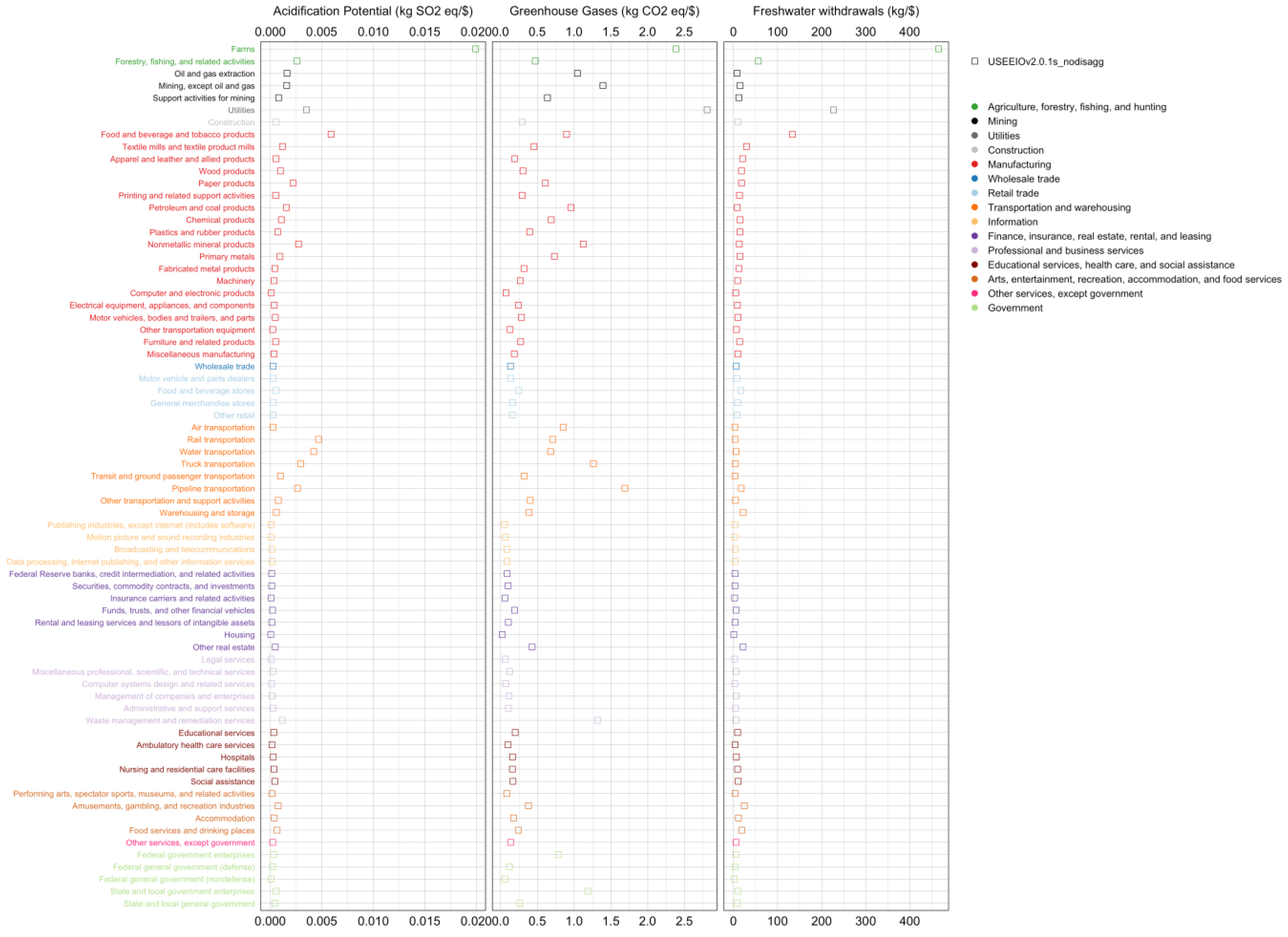
Total impact (direct + indirect) coefficients by sector, i.e.,
(see Equation (19)), are examined through the
plotMatrixCoefficient function. Results of three impact categories, including acidification potential (ACID), greenhouse gases (GHG), and freshwater withdrawals (WATR), are presented in
Figure 1. It should be noted that coefficients of these impact categories are generated using LCIA characterization factors from the TRACI2.1 method [
33]. The
farms sector has the largest ACID (0.02 kg SO
2 eq/USD) and WATR (460 kg/USD) coefficient, and the second largest GHG coefficient (2.4 kg CO2 eq/USD)—only smaller than that of the
utilities sector (2.8 kg SO
2 eq/USD), which is carbon intensive due to primarily fossil fuel-based electric power generation in the US.
Utilities also has a notably large WATR coefficient (230 kg/USD), for the same reason. Energy intensive sectors including resource exploitation (i.e.,
oil and gas extraction and
mining), manufacturing, transportation, and waste management sectors have relatively large GHG coefficients. This illustration provides a clear view of total impact coefficients by sector in the model year. With more environmental flow data over years, multiple snapshots of the illustration could reflect changes in impact coefficients potentially caused by technological advancement in industries, or structural changes in the economy.
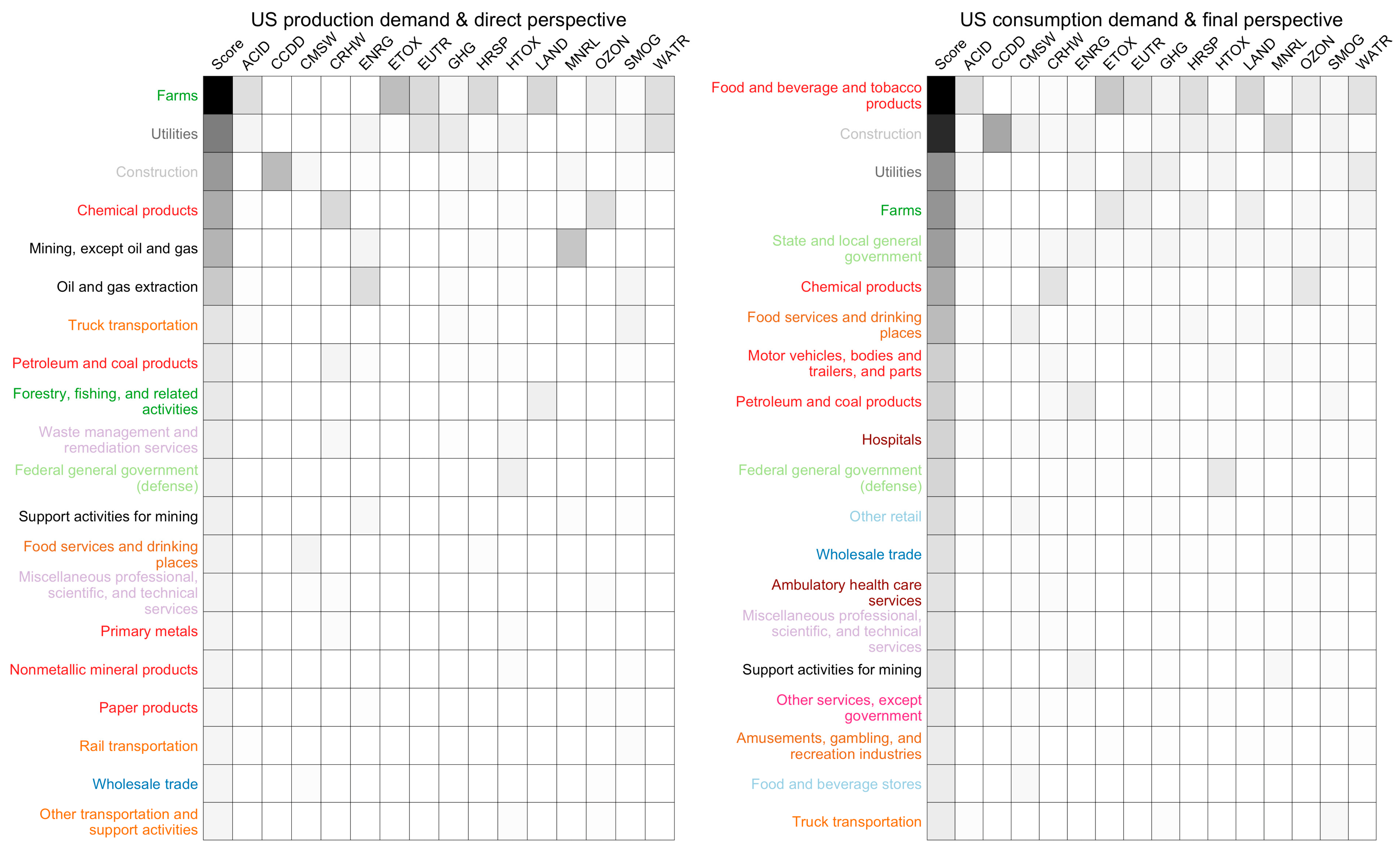
Ranking sectors based a composite score of selected total impacts associated with total US demand is an effective means to identify prioritization opportunity in practices, such as the EPA’s Sustainable Materials Management program. Comparing rankings is another form of model validation that incorporates the demand vectors and the indicators, as well as the matrices. The composite score for the rankings is calculated as a sum of fractions of sector impact relative to total impact across all sectors, by each selected indicator. This is represented using Equation (36), where
represents this score and
, calculated in Equation (37), is a vector of the column sums of the given
(see Equation (25)) matrix.
The first ranking uses
LCIAd with the US production vector (left in
Figure 2), while the second ranking is performed with
LCIAf (see Equation (27)), along with the US consumption vector (right in
Figure 2). The sets of commodities in the top 20 from the two rankings (left and right in
Figure 2) are nearly identical, with some notable substitutions and some exchanging of places.
Farms,
utilities, and
construction are in the top places in both rankings, but the orders and the distance (darkness of shade) separating
Construction from the other commodities are different.
Food and beverage and tobacco products is not in top 20 in the impact ranking created with
LCIAd and the US production vector (left), but is in the top place in the other impact ranking created with
LCIAf and the US consumption vector, as the latter calculation captures impacts, e.g., human health—respiratory effects (HRSP), associated with the use phase of commodities, e.g., tobacco.
Contribution from the top five flows to total acidification potential in the
Utilities sector is shown in
Table 2. As fossil fuels are still significant resources used by the
Utilities sector in the US, and sulfur dioxide and nitrogen dioxide emissions are the main cause for acidification potential, it is natural that they are the top two flows, and together contribute to more than 96% of the total impact. The other contributing flows are ammonia, sulfuric acid, and hydrofluoric acid, which together contribute to less than 4% to the total impact.
Contribution from the top five sectors to direct freshwater withdrawals in the
Food and beverage and tobacco products sector is shown in
Table 3. The
Farms sector contributes the most, because most inputs to the
Food and beverage and tobacco products sector come from
Farms. The
Utilities sector is in the second place, with less than 5% contribution, most likely due to water use in processing food, beverages, and tobacco products. The other contributing sectors are the
Food and beverage and tobacco products sector itself, which relates to by-products in the sector, the
Forestry, fishing, and related activities sector, which relates to seafood produced in the food sector, and the
Fabricated metal products sector, which most likely relates to canning of food and beverage.


