ALIPPF-Controller to Stabilize the Unstable Motion and Eliminate the Non-Linear Oscillations of the Rotor Electro-Magnetic Suspension System

Abstract

Within this work, an advanced control algorithm was proposed to eliminate the non-linear vibrations of the rotor electro-magnetic suspension system. The suggested control algorithm is known as the Adaptive Linear Integral Positive Position Feedback controller (ALIPPF-controller). The ALIPPF-controller is a combination of first-order and second-order filters that are coupled linearly to the targeted non-linear system in order to absorb the excessive vibratory energy. According to the introduced control strategy, the dynamical model of the controlled rotor system was established as six non-linear differential equations that are coupled linearly. The obtained dynamical model was investigated analytically applying the asymptotic analysis, where the slow-flow equations were extracted. Based on the derived slow-flow equations, the bifurcation behaviors of the controlled system were explored by plotting the different bifurcation diagrams. In addition, the performance of the ALIPPF-controller in eliminating the rotor lateral vibrations was compared with the conventional Positive Position Feedback (PPF) controller. The acquired results illustrated that the ALIPPF-controller is the best control technique that can eliminate the considered system’s lateral vibrations regardless of the angular speed and eccentricity of the rotating shaft. Finally, to demonstrate the accuracy of the obtained analytical results, numerical validation was performed for all obtained bifurcation diagrams that were in excellent agreement with the analytical solutions.

1. Introduction

The rotor electro-magnetic suspension system has been introduced as an optimal solution to get rid of the drawbacks of the conventional bearings system such as the limited operational speed, the existence of friction between the rotor and the bearings, and the need for continuous lubrication, etc. The rotor electro-magnetic suspension system is a type of bearing that supports the rotating shafts using an electro-magnetic levitation mechanism. The main working principle of the electro-magnetic levitation is to apply controllable magnetic forces that support the rotor system in its hovering position without physical contact with the stator. The operation of the rotor with the contactless feature has earned the electro-magnetic suspension system many advantages over the other conventional bearing mechanisms such as the lack of friction between the moving parts and the stator, high-speed operation, less maintenance, clean working environment with no need for lubrication, high reliability, high durability, etc. Accordingly, the rotor electro-magnetic suspension system was and still is one of the main research subjects for scientists and engineers worldwide, where many researchers have focused their work on investigating the dynamical characteristics of the different electro-magnetic suspension configurations. On the other hand, some researchers have introduced advanced control algorithms to enhance the dynamical behaviors of electro-magnetic suspension systems regardless of their configurations. Ji et al. [1] studied non-linear dynamics and the bifurcation behaviors of the four-pole electro-magnetic suspension system. They employed the asymptotic perturbation method along with the normal form technique to analyze the considered system. The authors reported that the four poles electro-magnetic suspension system may lose its stability via different types of bifurcations such as the Hopf and saddle node. Saeed et al. [2,3] discussed the vibration control and bifurcation elimination of the six-pole electro-magnetic suspension system utilizing the conventional PD-control technique. The authors studied two different configurations for the introduced controller. The first PD-control strategy has been designed based on the lateral displacements and lateral velocities of the rotor system, while the second control methodology is implemented based on the rotor radial oscillations. According to the studied control techniques, they concluded that the first control method is more efficient in mitigating the system lateral vibrations, while the second technique is more robust against the system instability. Ji et al. [4,5] investigated the non-linear oscillations of the eight-pole electro-magnetic suspension system controlled via the PD-control algorithm at the primary and super-harmonic resonances. The authors illustrated that the system has both complex bifurcation behavior and multiple fixed-point solutions. El-Shourbagy et al. [6] introduced a non-linear position-velocity control algorithm to enhance the dynamical characteristics and mitigate the vibratory motion of the eight-pole suspension system. Saeed et al. [7] explored the dynamics of the eight-poles electro-magnetic suspension system when the rub and impact occur between the moving parts and the rotor housing, where the obtained results showed that the rotor system may perform periodic, quasiperiodic, or chaotic motion depending on the impact stiffness magnitude and dynamic friction coefficient. Zhang et al. [8,9,10,11,12,13] extensively investigated the eight-pole suspension system with time-varying stiffness coefficients, where many non-linear phenomena have been reported such as the multi-pulse chaotic motion, saddle-node, and Hopf bifurcations. El-Shourbagy et al. [14] studied the 12-pole electro-magnetic suspension system utilizing the PD-controller. They investigated the effect of the different control parameters on the rotor stability charts. The acquired results showed that the system stability can be controlled using the proportional and derivative gain of the applied controller. Saeed and Kandil [15] introduced both the radial and cartesian proportional-derivative control methods to stabilize the 16-pole electro-magnetic suspension system. They derived the equations of motion according to the suggested control methodologies. In addition, perturbation analysis was employed to explore the system’s steady-state oscillation. Based on the obtained results, the authors confirmed that the radial control technique is more robust than the Cartesian one. In addition, extensive investigations of the 16-pole electro-magnetic suspension system with time-varying stiffness have been presented by Zhang and his coworkers [16,17,18,19,20]. Due to the flexibility of the electro-magnetic suspension system in adjusting its dynamical behavior according to the applied control algorithm, many researchers employed this suspension system as an active actuator to reshape the dynamics of some rotating machinery [21,22,23,24]. Ishida and Inoue [21] implemented a non-linear magnetic absorber based on the push–pull control mechanism to mitigate the lateral vibrations of a non-linear Jeffcott rotor system. Saeed et al. [22,23,24] applied a non-linear position-velocity control algorithm to enhance the dynamical characteristics of an asymmetric rotor system utilizing the four-pole electro-magnetic suspension system as an actuator.

One of the feasible control techniques that are applied extensively to suppress the non-linear oscillations of different dynamical systems is known as Positive Position Feedback (PPF) controller [25,26,27,28,29]. The PPF-controller is a second-order filter that couples to the targeted vibratory system linearly to suppress its undesired oscillation. Saeed et al. [29] applied the PPF-controller to mitigate the non-linear oscillation of the eight-pole electro-magnetic suspension system. The authors reported that the PPF-controller can eliminate the lateral oscillation of the rotor system at the perfect resonance conditions (i.e., when the rotor angular velocity is equal to the natural frequency of the suspension system); however, the PPF-controller can add more excessive vibratory energy to the rotor system rather than suppress it, if the perfect resonance conditions have been lost. Besides the PPF-controller, there is another efficient control algorithm known as the Linear Integral Resonant (LIR) controller that has been utilized to dampen the non-linear vibration of many dynamical systems [30,31,32,33,34,35,36,37,38]. The LIR-controller is a first-order filter that has been coupled to the targeted system to modify its linear damping coefficients, which ultimately mitigates the undesired oscillation. Saeed et al. [38] studied the vibration control of the electro-magnetic suspension system utilizing the LIR-controller. The authors reported that the integration of the LIR-controller to the rotor system can eliminate the non-linear bifurcations and mitigate the system vibration to respond as a linear system.

With this work, a modified version of the control algorithms that have the advantage of both the PPF-controller and LIR-controller has been investigated for the first time. The proposed control strategy is a combination of first-order and second-order filters that have been couped to the considered suspension system to reduce the undesired lateral oscillation. The main task of the second-order filter is to behave as a PPF-controller to eliminate the catastrophic oscillations of the considered system at the perfect resonance conditions, while the essential role of the first-order filter is to work as an LIR-controller that increases the controlled system linear damping, which ultimately removes the drawback of the PPF-controller when the resonance condition is lost. According to this philosophy, the whole system mathematical model was derived. Then, the established dynamical model was investigated analytically using asymptotic techniques [39,40,41,42,43,44,45]. The performance of the proposed control method in eliminating the non-linear oscillations of the considered suspension system was explored by plotting the different response curves. The obtained analytical and numerical results showed that the introduced control strategy can eliminate the rotor vibrations regardless of both the angular speed and eccentricity of the rotor system.

2. Equations of Motion

The considered rotor system is illustrated in Figure 1, where the rotating shaft is supported via eight electro-magnetic poles that serve as active magnetic bearings. The rotor system is assumed to be a rigid body with mass $m$ and eccentricity $e$ and rotates with angular speed $\upsilon$. Accordingly, the dynamical equations that govern the system’s lateral vibrations in $X_1$ and $X_2$ directions can be written as follows [46,47]:

$$m{\ddot{x}}_1-R_{X_1}=me {\upsilon }^2\cos (\upsilon t)$$

(1)

$$m{\ddot{x}}_2-R_{X_2}=me {\upsilon }^2\sin (\upsilon t)$$

(2)

where $R_{X_1}$ and $R_{X_2}$ denote the net restoring forces that are exerted on the rotating shaft due to the attractive electro-magnetic forces $h_j$ ($j=1,2,\dots ,8$). It is considered that the eight electro-magnetic poles are symmetric. Accordingly, the attractive magnetic force that is exerted on the rotor system due to each pole can be expressed as follows [47]:

$$h_j=\frac{1}{4}{\mu }_0{N}^{2}A\cos (\theta )\frac{I_j^2}{g_j^2}=\Delta \frac{I_j^2}{g_j^2},\hspace{1em}j=1\cdots 8$$

(3)

where $\mathsf{\Delta }=\frac{1}{4}{\mu }_0{N}^{2}A\cos \left(\theta \right)$ is constant (i.e., ${\mu }_0$ is the air permeability, $N$ is the winding number of the electrical coil of each pole, $A\cos \left(\theta \right)$ is the effective cross-sectional area of each pole), $I_j$ is the electrical current in the $j$ pole, and $g_j$ is the air-gap size between the rotating shaft and the $j$th pole. For the small displacements $x_1\left(t\right)$ and $x_2\left(t\right)$ of the rotating shaft within the pole housing, the instantaneous air-gap size $g_j$ between the rotating shaft and the $j$ pole can be expressed as follows:

$$\begin{array}{l}{g}_1(x_{1,}{x}_2)=s_0+x_1\sin (\alpha )-x_2\cos (\alpha ),\hspace{1em}{g}_2(x_{1,}{x}_2)=s_0+x_1\cos (\alpha )-x_2\sin (\alpha )\\ g_3(x_{1,}{x}_2)=s_0+x_1\cos (\alpha )+x_2\sin (\alpha ),\hspace{1em}{g}_4(x_{1,}{x}_2)=s_0+x_1\sin (\alpha )+x_2\cos (\alpha )\\ g_5(x_{1,}{x}_2)=s_0-x_1\sin (\alpha )+x_2\cos (\alpha ),\hspace{1em}{g}_6(x_{1,}{x}_2)=s_0-x_1\cos (\alpha )+x_2\sin (\alpha )\\ g_7(x_{1,}{x}_2)=s_0-x_1\cos (\alpha )-x_2\sin (\alpha ),\hspace{1em}{g}_8(x_{1,}{x}_2)=s_0-x_1\sin (\alpha )-x_2\cos (\alpha )\end{array}\}$$

(4)

where $s_0$ is the radial clearance between the rotating shaft and each electro-magnetic pole when the geometric center of both the rotor and pole housing coincided as shown in Figure 1a, and $2\alpha =45°$ is the angle between every two consecutive electro-magnetic poles. Based on the system geometry shown in Figure 1a,b, the electrical currents of the eight-pole are designed based on the push–pull control mechanism as follows:

$$I_1=I_8=I_0-i_{X_2},\hspace{1em}{I}_2=I_3=I_0+i_{X_1},\hspace{1em}{I}_4=I_5=I_0+i_{X_2},\hspace{1em}{I}_6=I_7=I_0-i_{X_1}$$

(5)

where $I_0$ is a per-magnetizing constant current, $i_{X_1}$, and $i_{X_2}$ are the control currents in $X_1$ and $X_2$ directions, respectively.

Within this article, a new control algorithm was proposed to eliminate the non-linear oscillations of the considered system beside the conventional PD-controller. The suggested new control technique is defined as the Linear Integral Positive Position Feedback controller (LIPPF-controller). Therefore, according to the introduced control strategy, the control currents $i_{X_1}$ and $i_{X_2}$ are designed as follows:

$$i_{X_1}=k_1{x}_1+k_2{\dot{x}}_1+k_3{x}_3+k_4{x}_5,\hspace{1em}{i}_{X_2}=k_1{x}_2+k_2{\dot{x}}_2+k_5{x}_4+k_6{x}_6$$

(6)

where $k_1$ and $k_2$ are the control gains of the conventional PD-controller. $k_3$ and $k_4$ are the control signal gains of the LIPPF-controller that is connected to the system oscillation mode in the $X_1$ direction. $k_5$ and $k_6$ are the control signal gains of the LIPPF-controller that is connected to the system oscillation mode in the $X_2$ direction.

The LIPPF-controller is a combination of both first-order and second-order filters that are excited linearly by the rotor system displacement, where the equations of motion of the proposed LIPPF-controller are given as follows:

$${\ddot{x}}_3+c_1{\dot{x}}_3+{\lambda }_1{x}_3={\delta }_1{x}_1$$

(7)

$${\ddot{x}}_4+c_2{\dot{x}}_4+{\lambda }_2{x}_4={\delta }_2{x}_2$$

(8)

$${\dot{x}}_5+{\lambda }_3{x}_5={\delta }_3{x}_1$$

(9)

$${\dot{x}}_6+{\lambda }_4{x}_6={\delta }_4{x}_2$$

(10)

where $c_1, c_2$ represent the linear damping coefficients, ${\lambda }_1, {\lambda }_2$ denote the natural frequency, and ${\lambda }_3, {\lambda }_4$ are the internal loop feedback gain of the suggested controller (i.e., LIPPF-controller). In addition, ${\delta }_1, {\delta }_2, {\delta }_3,$ and ${\delta }_4$ represent the feedback signal gains of the LIPPF-controller. The engineering implementation of the suggested control method is illustrated in Figure 2, where the instantaneous Cartesian displacements $x_1\left(t\right)$ and $x_2\left(t\right)$ of the rotor system are measured using proximity sensors. The measured signals are fed into a digital computer to manipulate them according to the proposed control strategy to form the control currents $i_{X_1}=k_1{x}_1+k_2{\dot{x}}_1+k_3{x}_3+k_4{x}_5$ and $i_{X_2}=k_1{x}_2+k_2{\dot{x}}_2+k_5{x}_4+k_6{x}_6$. Then, the electrical currents of the eight-pole (i.e., $I_1, I_2\dots ,I_8$) are applied via a power amplifier network as illustrated in Figure 2 in detail. Now to obtain the full mathematical model that governs the rotor and the controller dynamics, let us substitute Equations (4)–(6) into Equation (3), we get the restoring forces of the eight-pole as follows:

$$h_1=\Delta {\left(\frac{I_0-k_1{x}_2-k_2{\dot{x}}_2-k_5{x}_4-k_6{x}_6}{s_0+x_1\sin (\alpha )-x_2\cos (\alpha )}\right)}^2$$

(11)

$$h_2=\Delta {\left(\frac{I_0+k_1{x}_1+k_2{\dot{x}}_1+k_3{x}_3+k_4{x}_5}{s_0+x_1\cos (\alpha )-x_2\sin (\alpha )}\right)}^2$$

(12)

$$h_3=\Delta {\left(\frac{I_0+k_1{x}_1+k_2{\dot{x}}_1+k_3{x}_3+k_4{x}_5}{s_0+x_1\cos (\alpha )+x_2\sin (\alpha )}\right)}^2$$

(13)

$$h_4=\Delta {\left(\frac{I_0+k_1{x}_2+k_2{\dot{x}}_2+k_5{x}_4+k_6{x}_6}{s_0+x_1\sin (\alpha )+x_2\cos (\alpha )}\right)}^2$$

(14)

$$h_5=\Delta {\left(\frac{I_0+k_1{x}_2+k_2{\dot{x}}_2+k_5{x}_4+k_6{x}_6}{s_0-x_1\sin (\alpha )+x_2\cos (\alpha )}\right)}^2$$

(15)

$$h_6=\Delta {\left(\frac{I_0-k_1{x}_1-k_2{\dot{x}}_1-k_3{x}_3-k_4{x}_5}{s_0-x_1\cos (\alpha )+x_2\sin (\alpha )}\right)}^2$$

(16)

$$h_7=\Delta {\left(\frac{I_0-k_1{x}_1-k_2{\dot{x}}_1-k_3{x}_3-k_4{x}_5}{s_0-x_1\cos (\alpha )-x_2\sin (\alpha )}\right)}^2$$

(17)

$$h_8=\Delta {\left(\frac{I_0-k_1{x}_2-k_2{\dot{x}}_2-k_5{x}_4-k_6{x}_6}{s_0-x_1\sin (\alpha )-x_2\cos (\alpha )}\right)}^2$$

(18)

According to the orientations of the eight attractive forces $h_j$ ($j=1,2,\dots ,8$) shown in Figure 1, the net restoring forces $R_{X_1}$ and $R_{X_2}$ in $X_1$ and $X_2$ directions can be expressed as:

$$R_{X_1}=(h_6+h_7-h_2-h_3)\cos (\alpha )+(h_5+h_8-h_1-h_4)\sin (\alpha )$$

(19)

$$R_{X_2}=(h_1+h_8-h_4-h_5)\cos (\alpha )+(h_2+h_7-h_3-h_6)\sin (\alpha )$$

(20)

Substituting Equations (11)–(20) into Equations (1) and (2), with introducing the dimensionless variables and parameters: $y_1=\frac{x_1}{s_0}, y_2=\frac{x_2}{s_0}, y_3=\frac{x_3}{s_0}, y_4=\frac{x_4}{s_0}, y_5=\frac{x_5}{s_0}, y_6=\frac{x_6}{s_0}, \tau ={\omega }_{n}t, {\omega }_n=\sqrt{\Delta /m{s}_0^3}, p=\frac{s_0}{I_0}{k}_1, d=\frac{c_0{\omega }_n}{I_0}{k}_2, {\mu }_1=\frac{c_1}{2{\omega }_n}, {\mu }_2=\frac{c_2}{2{\omega }_n}, {\omega }_1=\sqrt{\frac{{\lambda }_1}{{\omega }_n^2}}, {\omega }_2=\sqrt{\frac{{\lambda }_2}{{\omega }_n^2}}, {\rho }_1=\frac{{\lambda }_3}{{\omega }_n}, {\rho }_2=\frac{{\lambda }_4}{{\omega }_n}, {\eta }_1=\frac{8s_0}{I_0}\cos \left(\alpha \right)k_3, {\eta }_2=\frac{8s_0}{I_0}\cos \left(\alpha \right)k_4, {\eta }_3=\frac{8s_0}{I_0}\cos \left(\alpha \right)k_5, {\eta }_4=\frac{8s_0}{I_0}\cos \left(\alpha \right)k_6, {\eta }_5=\frac{{\delta }_1}{{\omega }_n^2}, {\eta }_6=\frac{{\delta }_2}{{\omega }_n^2}, {\eta }_7=\frac{{\delta }_3}{{\omega }_n}, {\eta }_8=\frac{{\eta }_4}{{\omega }_n}, f=\frac{e}{s_0}, \Omega =\frac{\upsilon }{{\omega }_n}$, we have from Equations (1), (2) and (7)–(10) the following dimensionless equations of motion:

$$\begin{array}{l}{\ddot{y}}_1+2\mu {\dot{y}}_1+{\omega }^2{y}_1-({\alpha }_1{y}_1^3+{\alpha }_2{y}_1{y}_2^2+{\alpha }_3{y}_1^2{\dot{y}}_1+{\alpha }_4{\dot{y}}_1{y}_2^2+{\alpha }_5{y}_1{\dot{y}}_2^2+{\alpha }_6{y}_1{\dot{y}}_1^2\\ +{\alpha }_7{y}_1{y}_2{\dot{y}}_2+{\beta }_1{y}_1^2{y}_3+{\beta }_2{y}_1{\dot{y}}_1{y}_3+{\beta }_3{y}_1{y}_3^2+{\beta }_4{y}_1{y}_2{y}_4+{\beta }_5{y}_1{y}_4^2+{\beta }_6{y}_1{\dot{y}}_2{y}_4\\ +{\beta }_7{y}_2^2{y}_3+{\beta }_8{y}_1{y}_3{y}_5+{\beta }_9{y}_1{\dot{y}}_1{y}_5+{\beta }_{10}{y}_1{y}_4{y}_6+{\beta }_{11}{y}_1^2{y}_5+{\beta }_{12}{y}_1{y}_6^2+{\beta }_{13}{y}_1{y}_2{y}_6\\ +{\beta }_{14}{y}_1{\dot{y}}_2{y}_6+{\beta }_{15}{y}_1{y}_5^2+{\beta }_{16}{y}_2^2{y}_5)=f{\Omega }^2\cos (\Omega \tau )+{\eta }_1{y}_3+{\eta }_2{y}_5\end{array}$$

(21)

$$\begin{array}{l}{\ddot{y}}_2+2\mu {\dot{y}}_2+{\omega }^2{y}_2-({\alpha }_1{y}_2^3+{\alpha }_2{y}_2{y}_1^2+{\alpha }_3{y}_2^2{\dot{y}}_2+{\alpha }_4{\dot{y}}_2{y}_1^2+{\alpha }_5{y}_2{\dot{y}}_1^2+{\alpha }_6{y}_2{\dot{y}}_2^2\\ +{\alpha }_7{y}_2{y}_1{\dot{y}}_1+{\gamma }_1{y}_2^2{y}_4+{\gamma }_2{y}_2{\dot{y}}_2{y}_4+{\gamma }_3{y}_2{y}_4^2+{\gamma }_4{y}_2{y}_1{y}_3+{\gamma }_5{y}_2{y}_3^2+{\gamma }_6{y}_2{\dot{y}}_1{y}_3\\ +{\gamma }_7{y}_4{y}_1^2+{\gamma }_8{y}_2{y}_4{y}_6+{\gamma }_9{y}_2{\dot{y}}_2{y}_6+{\gamma }_{10}{y}_2{y}_3{y}_5+{\gamma }_{11}{y}_2^2{y}_6+{\gamma }_{12}{y}_2{y}_5^2+{\gamma }_{13}{y}_2{y}_1{y}_5\\ +{\gamma }_{14}{y}_2{\dot{y}}_1{y}_5+{\gamma }_{15}{y}_2{y}_6^2+{\gamma }_{16}{y}_1^2{y}_6)=f{\Omega }^2\sin (\Omega \tau )+{\eta }_3{y}_4+{\eta }_4{y}_6\end{array}$$

(22)

$${\ddot{y}}_3+2{\mu }_1{\dot{y}}_3+{\omega }_1^2{y}_3={\eta }_5{y}_1$$

(23)

$${\ddot{y}}_4+2{\mu }_2{\dot{y}}_4+{\omega }_2^2{y}_4={\eta }_6{y}_2$$

(24)

$${\dot{y}}_5+{\rho }_1{y}_5={\eta }_7{y}_1$$

(25)

$${\dot{y}}_6+{\rho }_2{y}_6={\eta }_8{y}_2$$

(26)

where Equations (21) and (22) represent the equations of motion of the controller rotor system, while Equations (23)–(26) are the equations of the coupled LIPPF-controller. The coefficients of Equations (21)–(26) are given in the Appendix A.

3. Analytical Investigations

To evaluate the performance of the suggested control method (i.e., LIPPF-controller) in eliminating the non-linear oscillations of the studied rotor-magnetic bearings system, an analytical solution for Equations (21)–(26) is sought by applying the perturbation analysis as follows [39,40]:

$$y_1(\tau ,\epsilon )=y_{10}(T_0,T_1)+\epsilon y_{11}(T_0,T_1)+O({\epsilon }^2)$$

(27)

$$y_2(\tau ,\epsilon )=y_{20}(T_0,T_1)+\epsilon y_{21}(T_0,T_1)+O({\epsilon }^2)$$

(28)

$$y_3(\tau ,\epsilon )=y_{30}(T_0,T_1)+\epsilon y_{31}(T_0,T_1)+O({\epsilon }^2)$$

(29)

$$y_4(\tau ,\epsilon )=y_{40}(T_0,T_1)+\epsilon y_{41}(T_0,T_1)+O({\epsilon }^2)$$

(30)

$$y_5(\tau ,\epsilon )=\epsilon y_{50}(T_0,T_1)+{\epsilon }^2{y}_{51}(T_0,T_1)+O({\epsilon }^2)$$

(31)

$$y_6(\tau ,\epsilon )=\epsilon y_{60}(T_0,T_1)+{\epsilon }^2{y}_{61}(T_0,T_1)+O({\epsilon }^2)$$

(32)

where $T_0=\tau$, $T_1=\epsilon \tau$, and $\epsilon$ is called a perturbation parameter used as a book-keeping parameter only through this work [40]. Accordingly, the ordinary derivatives $\frac{d}{d\tau }$ and $\frac{d^2}{d{\tau }^2}$ can be expressed in terms of $T_0$ and $T_1$ as follows:

$$\frac{d}{d\tau }=D_0+\epsilon D_1, \frac{d^2}{d{\tau }^2}=D_0^2+2\epsilon D_0{D}_1, D_j=\frac{\partial }{\partial T_j},\hspace{1em}j=0,1$$

(33)

To perform the perturbation procedure, the parameters of Equations (21)–(26) should be scaled as follows:

$$\begin{array}{l}f=\epsilon \tilde{f},\hspace{1em}\mu =\epsilon \tilde{\mu },\hspace{1em}{\mu }_1=\epsilon {\tilde{\mu }}_1,\hspace{1em}{\mu }_2=\epsilon {\tilde{\mu }}_2,\hspace{1em}{\alpha }_j=\epsilon {\tilde{\alpha }}_j,\hspace{1em}{\beta }_j=\epsilon {\tilde{\beta }}_j,\hspace{1em}{\gamma }_j=\epsilon {\tilde{\gamma }}_j,\hspace{1em}{\eta }_k=\epsilon {\tilde{\eta }}_k,\\ j=1,2,\cdots ,7;\hspace{1em}k=1,3,5,6,7,8.\end{array}$$

(34)

Substituting Equations (27)–(34) into Equations (21)–(26) with expanding the resulting equations and comparing the coefficients of the same power of $\epsilon$, yields $O\left({\epsilon }^0\right):$

$$(D_0^2+{\omega }^2)y_{10}=0$$

(35)

$$(D_0^2+{\omega }^2)y_{20}=0$$

(36)

$$(D_0^2+{\omega }_1^2)y_{30}=0$$

(37)

$$(D_0^2+{\omega }_2^2)y_{40}=0$$

(38)

$O\left({\epsilon }^1\right)$:

$$\begin{array}{ll}(D_0^2+{\omega }^2)y_{11}& =-2D_0{D}_1{y}_{10}-2\tilde{\mu }{D}_0{y}_{10}+{\tilde{\alpha }}_1{y}_{10}^3+{\tilde{\alpha }}_2{y}_{10}{y}_{20}^2+{\tilde{\alpha }}_3{y}_{10}^2{D}_0{y}_{10}+{\tilde{\alpha }}_4{y}_{20}^2{D}_0{y}_{10}\\ & +{\tilde{\alpha }}_5{y}_{10}{(D_0{y}_{20})}^2+{\tilde{\alpha }}_6{y}_{10}{(D_0{y}_{10})}^2+{\tilde{\alpha }}_7{y}_{10}{y}_{20}{D}_0{y}_{20}+{\tilde{\beta }}_1{y}_{10}^2{y}_{30}+{\tilde{\beta }}_2{y}_{10}{D}_0{y}_{10}{y}_{30}\\ & +{\tilde{\beta }}_3{y}_{10}{y}_{30}^2+{\tilde{\beta }}_4{y}_{10}{y}_{20}{y}_{40}+{\tilde{\beta }}_5{y}_{10}{y}_{40}^2+{\tilde{\beta }}_6{y}_{10}{D}_0{y}_{20}{y}_{40}+{\tilde{\beta }}_7{y}_{20}^2{y}_{30}+{\beta }_8{y}_{10}{y}_{30}{y}_{50}\\ & +{\beta }_9{y}_{10}{D}_0{y}_{10}{y}_{50}+{\beta }_{10}{y}_{10}{y}_{40}{y}_{60}+{\beta }_{11}{y}_{10}^2{y}_{50}+{\beta }_{12}{y}_{10}{y}_{60}^2+{\beta }_{13}{y}_{10}{y}_{20}{y}_{60}\\ & +{\beta }_{14}{y}_{10}{D}_0{y}_{20}{y}_{60}+{\beta }_{15}{y}_{10}{y}_{50}^2+{\beta }_{16}{y}_{20}^2{y}_{50}+{\Omega }^2\tilde{f}\cos (\Omega T_0)+{\tilde{\eta }}_1{y}_{30}+{\eta }_2{y}_{50}\end{array}$$

(39)

$$\begin{array}{ll}(D_0^2+{\omega }^2)y_{21}& =-2D_0{D}_1{y}_{20}-2\tilde{\mu }{D}_0{y}_{20}+{\tilde{\alpha }}_1{y}_{20}^3+{\tilde{\alpha }}_2{y}_{20}{y}_{10}^2+{\tilde{\alpha }}_3{y}_{20}^2(D_0{y}_{20})+{\tilde{\alpha }}_4{y}_{10}^2(D_0{y}_{20})\\ & +{\tilde{\alpha }}_5{y}_{20}{(D_0{y}_{10})}^2+{\tilde{\alpha }}_6{y}_{20}{(D_0{y}_{20})}^2+{\tilde{\alpha }}_7{y}_{20}{y}_{10}(D_0{y}_{10})+{\tilde{\gamma }}_1{y}_{20}^2{y}_{40}+{\tilde{\gamma }}_2{y}_{20}(D_0{y}_{20})y_{40}\\ & +{\tilde{\gamma }}_3{y}_{20}{y}_{40}^2+{\tilde{\gamma }}_4{y}_{20}{y}_{10}{y}_{30}+{\tilde{\gamma }}_5{y}_{20}{y}_{30}^2+{\tilde{\gamma }}_6{y}_{20}(D_0{y}_{10})y_{30}+{\tilde{\gamma }}_7{y}_{10}^2{y}_{40}+{\gamma }_8{y}_{20}{y}_{40}{y}_{60}\\ & +{\gamma }_9{y}_{20}(D_0{y}_{20})y_{60}+{\gamma }_{10}{y}_{20}{y}_{30}{y}_{50}+{\gamma }_{11}{y}_{20}^2{y}_{60}+{\gamma }_{12}{y}_{20}{y}_{50}^2+{\gamma }_{13}{y}_{20}{y}_{10}{y}_{50}\\ & +{\gamma }_{14}{y}_{20}(D_0{y}_{10})y_{50}+{\gamma }_{15}{y}_{20}{y}_{60}^2+{\gamma }_{16}{y}_{10}^2{y}_{60}+\tilde{f}{\Omega }^2\sin (\Omega T_0)+{\tilde{\eta }}_3{y}_{40}+{\eta }_4{y}_{60}\end{array}$$

(40)

$$(D_0^2+{\omega }_1^2)y_{31}=-2D_0{D}_1{y}_{30}-2\epsilon {\tilde{\mu }}_1{D}_0{y}_{30}+{\tilde{\eta }}_5{y}_{10}$$

(41)

$$(D_0^2+{\omega }_2^2)y_{41}=-2D_0{D}_1{y}_{40}-2{\tilde{\mu }}_2{D}_0{y}_{40}+{\tilde{\eta }}_6{y}_{20}$$

(42)

$$(D_0+{\rho }_1)y_{50}={\tilde{\eta }}_7{y}_{10}$$

(43)

$$(D_0+{\rho }_2)y_{60}={\tilde{\eta }}_8{y}_{20}$$

(44)

The steady-state solutions of Equations (35)–(37), (43) and (44) can be written as follows:

$$y_{10}(T_0,T_1)=A_1(T_1)e^{i\omega T_0}+{\overline{A}}_1(T_1)e^{-i\omega T_0}$$

(45)

$$y_{20}(T_0,T_1)=A_2(T_1)e^{i\omega T_0}+{\overline{A}}_2(T_1)e^{-i\omega T_0}$$

(46)

$$y_{30}(T_0,T_1)=B_1(T_1)e^{i{\omega }_1{T}_0}+{\overline{B}}_1(T_1)e^{-i{\omega }_1{T}_0}$$

(47)

$$y_{40}(T_0,T_1)=B_2(T_1)e^{i{\omega }_2{T}_0}+{\overline{B}}_2(T_1)e^{-i{\omega }_2{T}_0}$$

(48)

$$y_{50}(T_0,T_1)={\psi }_1{A}_1(T_1)e^{i\omega T_0}+{\overline{\psi }}_1{\overline{A}}_1(T_1)e^{-i\omega T_0}$$

(49)

$$y_{60}(T_0,T_1)={\psi }_2{A}_2(T_1)e^{i\omega T_0}+{\overline{\psi }}_2{\overline{A}}_2(T_1)e^{-i\omega T_0}$$

(50)

where $i=\sqrt{-1}, A_1\left(T_1\right), A_2\left(T_1\right), B_1\left(T_1\right),$ and $B_2\left(T_1\right)$ are unknown functions that will be determined next. ${\overline{A}}_1\left(T_1\right), {\overline{A}}_2\left(T_1\right), {\overline{B}}_1\left(T_1\right),$ and ${\overline{B}}_2\left(T_1\right)$ are the complex conjugate functions of $A_1\left(T_1\right), A_2\left(T_1\right), B_1\left(T_1\right),$ and $B_2\left(T_1\right)$, respectively. ${\psi }_1=\frac{{\rho }_1-i\omega }{{\rho }_1^2+{\omega }^2}{\widehat{\eta }}_7,{\overline{ \psi }}_1=\frac{{\rho }_1+i\omega }{{\rho }_1^2+{\omega }^2}{\widehat{\eta }}_7, {\psi }_2=\frac{{\rho }_2-i\omega }{{\rho }_2^2+{\omega }^2}{\widehat{\eta }}_8,$ and ${\overline{\psi }}_2=\frac{{\rho }_2+i\omega }{{\rho }_2^2+{\omega }^2}{\widehat{\eta }}_8$. Substituting Equations (45)–(50) into Equations (39)–(42), yields

$$\begin{array}{ll}(D_0^2+{\omega }^2)y_{11}& =(-2i\omega D_1{A}_1-2i\tilde{\mu }\omega A_1+3{\tilde{\alpha }}_1{A}_1^2{\overline{A}}_1+2{\tilde{\alpha }}_2{A}_1{A}_2{\overline{A}}_2+{\tilde{\alpha }}_2{\overline{A}}_1{A}_2^2+i{\tilde{\alpha }}_3\omega A_1^2{\overline{A}}_1\\ & +2i{\tilde{\alpha }}_4\omega A_1{A}_2{\overline{A}}_2-i{\tilde{\alpha }}_4\omega {\overline{A}}_1{A}_2^2+2{\tilde{\alpha }}_5{\omega }^2{A}_1{A}_2{\overline{A}}_2-{\tilde{\alpha }}_5{\omega }^2{\overline{A}}_1{A}_2^2+{\tilde{\alpha }}_6{\omega }^2{A}_1^2{\overline{A}}_1\\ & +i{\tilde{\alpha }}_7\omega {\overline{A}}_1{A}_2^2+2{\tilde{\beta }}_3{A}_1{B}_1{\overline{B}}_1+2{\tilde{\beta }}_5{A}_1{B}_2{\overline{B}}_2+2{\beta }_{11}{\psi }_1{A}_1^2{\overline{A}}_1+{\beta }_{12}{\psi }_2^2{\overline{A}}_1{A}_2^2\\ & +{\beta }_{13}{\psi }_2{A}_1{A}_2{\overline{A}}_2+{\beta }_{13}{\psi }_2{\overline{A}}_1{A}_2^2-i{\beta }_{14}\omega {\psi }_2{A}_1{A}_2{\overline{A}}_2+i{\beta }_{14}\omega {\psi }_2{\overline{A}}_1{A}_2^2\\ & +{\beta }_{15}{\psi }_1^2{A}_1^2{\overline{A}}_1+2{\beta }_{16}{\psi }_1{A}_1{A}_2{\overline{A}}_2+{\eta }_2{\psi }_1{A}_1)e^{i\omega T_0}+{\tilde{\eta }}_1{B}_1{e}^{i{\omega }_1{T}_0}+({\tilde{\alpha }}_1{A}_1^3\\ & +{\tilde{\alpha }}_2{A}_1{A}_2^2+i{\tilde{\alpha }}_3\omega A_1^3+i{\tilde{\alpha }}_4\omega A_1{A}_2^2-{\tilde{\alpha }}_5{\omega }^2{A}_1{A}_2^2-{\tilde{\alpha }}_6{\omega }^2{A}_1^3+i{\tilde{\alpha }}_7\omega A_1{A}_2^2\\ & +i{\beta }_9\omega {\psi }_1{A}_1^3+{\beta }_{11}{\psi }_1{A}_1^3+{\beta }_{12}{\psi }_2^2{A}_1{A}_2^2+{\beta }_{13}{\psi }_2{A}_1{A}_2^2+i{\beta }_{14}\omega {\psi }_2{A}_1{A}_2^2\\ & +{\beta }_{15}{\psi }_1^2{A}_1^3+{\beta }_{16}{\psi }_1{A}_1{A}_2^2)e^{3i\omega T_0}+({\tilde{\beta }}_1{A}_1^2{B}_1+i{\tilde{\beta }}_2\omega A_1^2{B}_1+{\tilde{\beta }}_7{A}_2^2{B}_1\\ & +{\beta }_8{\psi }_1{A}_1^2{B}_1)e^{i(2\omega +{\omega }_1)T_0}+({\tilde{\beta }}_1{A}_1^2{\overline{B}}_1+i{\tilde{\beta }}_2\omega A_1^2{\overline{B}}_1+{\tilde{\beta }}_7{A}_2^2{\overline{B}}_1\\ & +{\beta }_8{\psi }_1{A}_1^2{\overline{B}}_1)e^{i(2\omega -{\omega }_1)T_0}+(2{\tilde{\beta }}_1{A}_1{\overline{A}}_1{B}_1+2{\tilde{\beta }}_7{A}_2{\overline{A}}_2{B}_1+{\beta }_8{\psi }_1{A}_1{\overline{A}}_1{B}_1)e^{i{\omega }_1{T}_0}\\ & +{\tilde{\beta }}_3{A}_1{B}_1^2{e}^{i(\omega +2{\omega }_1)T_0}+{\tilde{\beta }}_3{\overline{A}}_1{B}_1^2{e}^{i(2{\omega }_1-\omega )T_0}+({\tilde{\beta }}_4{A}_1{A}_2{B}_2+i{\tilde{\beta }}_6\omega A_1{A}_2{B}_2\\ & +{\beta }_{10}{\psi }_2{A}_1{A}_2{B}_2)e^{i(2\omega +{\omega }_2)T_0}+({\tilde{\beta }}_4{A}_1{A}_2{\overline{B}}_2+i{\tilde{\beta }}_6\omega A_1{A}_2{\overline{B}}_2\\ & +{\beta }_{10}{\psi }_2{A}_1{A}_2{\overline{B}}_2)e^{i(2\omega -{\omega }_2)T_0}+({\tilde{\beta }}_4{A}_1{\overline{A}}_2{B}_2+{\tilde{\beta }}_4{\overline{A}}_1{A}_2{B}_2-i{\tilde{\beta }}_6\omega A_1{\overline{A}}_2{B}_2\\ & +i{\tilde{\beta }}_6\omega {\overline{A}}_1{A}_2{B}_2+{\beta }_{10}{\psi }_2{\overline{A}}_1{A}_2{B}_2)e^{i{\omega }_2{T}_0}+{\tilde{\beta }}_5{A}_1{B}_2^2{e}^{i(\omega +2{\omega }_2)T_0}+{\tilde{\beta }}_5{\overline{A}}_1{B}_2^2{e}^{i(2{\omega }_2-\omega )T_0}\\ & +\frac{1}{2}{\Omega }^2\tilde{f}{e}^{i\Omega T_0}+cc\end{array}$$

(51)

$$\begin{array}{ll}(D_0^2+{\omega }^2)y_{21}& =(-2i\omega D_1{A}_2-2i\tilde{\mu }\omega A_2+3{\tilde{\alpha }}_1{A}_2^2{\overline{A}}_2+2{\tilde{\alpha }}_2{A}_2{A}_1{\overline{A}}_1+{\tilde{\alpha }}_2{\overline{A}}_2{A}_1^2+i{\tilde{\alpha }}_3\omega A_2^2{\overline{A}}_2\\ & +2i{\tilde{\alpha }}_4\omega A_2{A}_1{\overline{A}}_1-i{\tilde{\alpha }}_4\omega {\overline{A}}_2{A}_1^2+2{\tilde{\alpha }}_5{\omega }^2{A}_2{A}_1{\overline{A}}_1-{\tilde{\alpha }}_5{\omega }^2{\overline{A}}_2{A}_1^2+{\tilde{\alpha }}_6{\omega }^2{A}_2^2{\overline{A}}_2\\ & +i{\tilde{\alpha }}_7\omega {\overline{A}}_2{A}_1^2+2{\tilde{\gamma }}_3{A}_2{B}_2{\overline{B}}_2+2{\tilde{\gamma }}_5{A}_2{B}_1{\overline{B}}_1+2{\gamma }_{11}{\psi }_2{A}_2^2{\overline{A}}_2+{\gamma }_{12}{\psi }_1^2{\overline{A}}_2{A}_1^2\\ & +{\gamma }_{13}{\psi }_1{A}_2{A}_1{\overline{A}}_1+{\gamma }_{13}{\psi }_1{\overline{A}}_2{A}_1^2-i{\gamma }_{14}\omega {\psi }_1{A}_2{A}_1{\overline{A}}_1+i{\gamma }_{14}\omega {\psi }_1{\overline{A}}_2{A}_1^2\\ & +{\gamma }_{15}{\psi }_2^2{A}_2^2{\overline{A}}_2+2{\gamma }_{16}{\psi }_2{A}_2{A}_1{\overline{A}}_1+{\eta }_4{\psi }_2{A}_2)e^{i\omega T_0}+{\tilde{\eta }}_3{B}_2{e}^{i{\omega }_2{T}_0}+({\tilde{\alpha }}_1{A}_2^3\\ & +{\tilde{\alpha }}_2{A}_2{A}_1^2+i{\tilde{\alpha }}_3\omega A_2^3+i{\tilde{\alpha }}_4\omega A_2{A}_1^2-{\tilde{\alpha }}_5{\omega }^2{A}_2{A}_1^2-{\tilde{\alpha }}_6{\omega }^2{A}_2^3+i{\tilde{\alpha }}_7\omega A_2{A}_1^2\\ & +i{\gamma }_9\omega {\psi }_2{A}_2^3+{\gamma }_{11}{\psi }_2{A}_2^3+{\gamma }_{12}{\psi }_1^2{A}_2{A}_1^2+{\gamma }_{13}{\psi }_1{A}_2{A}_1^2+i{\gamma }_{14}\omega {\psi }_1{A}_2{A}_1^2\\ & +{\gamma }_{15}{\psi }_2^2{A}_2^3+{\gamma }_{16}{\psi }_2{A}_2{A}_1^2)e^{3i\omega T_0}+({\tilde{\gamma }}_1{A}_2^2{B}_2+i{\tilde{\gamma }}_2\omega A_2^2{B}_2+{\tilde{\gamma }}_7{A}_1^2{B}_2\\ & +{\gamma }_8{\psi }_2{A}_2^2{B}_2)e^{i(2\omega +{\omega }_2)T_0}+({\tilde{\gamma }}_1{A}_2^2{\overline{B}}_2+i{\tilde{\gamma }}_2\omega A_2^2{\overline{B}}_2+{\tilde{\gamma }}_7{A}_1^2{\overline{B}}_2\\ & +{\gamma }_8{\psi }_2{A}_2^2{\overline{B}}_2)e^{i(2\omega -{\omega }_2)T_0}+(2{\tilde{\gamma }}_1{A}_2{\overline{A}}_2{B}_2+2{\tilde{\gamma }}_7{A}_1{\overline{A}}_1{B}_2+{\gamma }_8{\psi }_2{A}_2{\overline{A}}_2{B}_2)e^{i{\omega }_2{T}_0}\\ & +{\tilde{\gamma }}_3{A}_2{B}_2^2{e}^{i(\omega +2{\omega }_2)T_0}+{\tilde{\gamma }}_3{\overline{A}}_2{B}_2^2{e}^{i(2{\omega }_2-\omega )T_0}+({\tilde{\gamma }}_4{A}_2{A}_1{B}_1+i{\tilde{\gamma }}_6\omega A_2{A}_1{B}_1\\ & +{\gamma }_{10}{\psi }_1{A}_2{A}_1{B}_1)e^{i(2\omega +{\omega }_1)T_0}+({\tilde{\gamma }}_4{A}_2{A}_1{\overline{B}}_1+i{\tilde{\gamma }}_6\omega A_2{A}_1{\overline{B}}_1+{\gamma }_{10}{\psi }_1{\overline{A}}_2{A}_1{\overline{B}}_1)e^{i(2\omega -{\omega }_1)T_0}\\ & +({\tilde{\gamma }}_4{A}_2{\overline{A}}_1{B}_1+{\tilde{\gamma }}_4{\overline{A}}_2{A}_1{B}_1-i{\tilde{\gamma }}_6\omega A_2{\overline{A}}_1{B}_1+i{\tilde{\gamma }}_6\omega {\overline{A}}_2{A}_1{B}_1+{\gamma }_{10}{\psi }_1{A}_2{A}_1{B}_1)e^{i{\omega }_1{T}_0}\\ & +{\tilde{\gamma }}_5{A}_2{B}_1^2{e}^{i(\omega +2{\omega }_1)T_0}+{\tilde{\gamma }}_5{\overline{A}}_2{B}_1^2{e}^{i(2{\omega }_1-\omega )T_0}-\frac{1}{2}i{\Omega }^2\tilde{f}{e}^{i\Omega T_0}+cc\end{array}$$

(52)

$$(D_0^2+{\omega }_1^2)y_{31}=-2i{\omega }_1{D}_1{B}_1{e}^{i{\omega }_1{T}_0}-2i{\tilde{\mu }}_1{\omega }_1{B}_1{e}^{i{\omega }_1{T}_0}+{\tilde{\eta }}_5{A}_1{e}^{i\omega T_0}+cc$$

(53)

$$(D_0^2+{\omega }_2^2)y_{41}=-2i{\omega }_2{D}_1{B}_2{e}^{i{\omega }_2{T}_0}-2i{\tilde{\mu }}_2{\omega }_2{B}_2{e}^{i{\omega }_2{T}_0}+{\tilde{\eta }}_6{A}_2{e}^{i\omega T_0}+cc$$

(54)

where $cc$ denotes the complex conjugate terms. To get a bounded solution for Equations (51)–(54), the small divisor and secular terms in these equations should vanish. Accordingly, to get the small divisor at the primary resonance cases, let $\sigma , {\sigma }_1,$ and ${\sigma }_2$ to describe the closeness of $\Omega , {\omega }_1,$ and ${\omega }_2$ to the rotor natural frequency $\omega$ as follows:

$$\Omega =\omega +\sigma ,\hspace{1em}{\omega }_1=\omega +{\sigma }_1,\hspace{1em}{\omega }_2=\omega +{\sigma }_2$$

(55)

Substituting Equation (55) into Equations (51)–(54), one can obtain the solvability conditions of Equations (51)–(54) as follows:

$$\begin{array}{l}-2i\omega D_1{A}_1-2i\tilde{\mu }\omega A_1+3{\tilde{\alpha }}_1{A}_1^2{\overline{A}}_1+2{\tilde{\alpha }}_2{A}_1{A}_2{\overline{A}}_2+{\tilde{\alpha }}_2{\overline{A}}_1{A}_2^2+i{\tilde{\alpha }}_3\omega A_1^2{\overline{A}}_1+2i{\tilde{\alpha }}_4\omega A_1{A}_2{\overline{A}}_2\\ -i{\tilde{\alpha }}_4\omega {\overline{A}}_1{A}_2^2+2{\tilde{\alpha }}_5{\omega }^2{A}_1{A}_2{\overline{A}}_2-{\tilde{\alpha }}_5{\omega }^2{\overline{A}}_1{A}_2^2+{\tilde{\alpha }}_6{\omega }^2{A}_1^2{\overline{A}}_1+i{\tilde{\alpha }}_7\omega {\overline{A}}_1{A}_2^2+2{\tilde{\beta }}_3{A}_1{B}_1{\overline{B}}_1\\ +2{\tilde{\beta }}_5{A}_1{B}_2{\overline{B}}_2+2{\beta }_{11}{\psi }_1{A}_1^2{\overline{A}}_1+{\beta }_{12}{\psi }_2^2{\overline{A}}_1{A}_2^2+{\beta }_{13}{\psi }_2{A}_1{A}_2{\overline{A}}_2+{\beta }_{13}{\psi }_2{\overline{A}}_1{A}_2^2-i{\beta }_{14}\omega {\psi }_2{A}_1{A}_2{\overline{A}}_2\\ +i{\beta }_{14}\omega {\psi }_2{\overline{A}}_1{A}_2^2+{\beta }_{15}{\psi }_1^2{A}_1^2{\overline{A}}_1+2{\beta }_{16}{\psi }_1{A}_1{A}_2{\overline{A}}_2+{\tilde{\eta }}_1{B}_1{e}^{i{\sigma }_1{T}_0}+{\eta }_2{\psi }_1{A}_1+({\tilde{\beta }}_1{A}_1^2{\overline{B}}_1+i{\tilde{\beta }}_2\omega A_1^2{\overline{B}}_1\\ +{\tilde{\beta }}_7{A}_2^2{\overline{B}}_1+{\beta }_8{\psi }_1{A}_1^2{\overline{B}}_1)e^{-i{\sigma }_1{T}_0}+(2{\tilde{\beta }}_1{A}_1{\overline{A}}_1{B}_1+2{\tilde{\beta }}_7{A}_2{\overline{A}}_2{B}_1+{\beta }_8{\psi }_1{A}_1{\overline{A}}_1{B}_1)e^{i{\sigma }_1{T}_0}+({\tilde{\beta }}_4{A}_1{A}_2{\overline{B}}_2\\ +i{\tilde{\beta }}_6\omega A_1{A}_2{\overline{B}}_2+{\beta }_{10}{\psi }_2{A}_1{A}_2{\overline{B}}_2)e^{-i{\sigma }_2{T}_0}+{\tilde{\beta }}_3{\overline{A}}_1{B}_1^2{e}^{2i{\sigma }_1{T}_0}+({\tilde{\beta }}_4{A}_1{\overline{A}}_2{B}_2+{\tilde{\beta }}_4{\overline{A}}_1{A}_2{B}_2-i{\tilde{\beta }}_6\omega A_1{\overline{A}}_2{B}_2\\ +i{\tilde{\beta }}_6\omega {\overline{A}}_1{A}_2{B}_2+{\beta }_{10}{\psi }_2{\overline{A}}_1{A}_2{B}_2)e^{i{\sigma }_2{T}_0}+{\tilde{\beta }}_5{\overline{A}}_1{B}_2^2{e}^{2i{\sigma }_2{T}_0}+\frac{1}{2}{(\omega +\sigma )}^2\tilde{f}{e}^{i\sigma T_0}=0\end{array}$$

(56)

$$\begin{array}{l}-2i\omega D_1{A}_2-2i\tilde{\mu }\omega A_2+3{\tilde{\alpha }}_1{A}_2^2{\overline{A}}_2+2{\tilde{\alpha }}_2{A}_2{A}_1{\overline{A}}_1+{\tilde{\alpha }}_2{\overline{A}}_2{A}_1^2+i{\tilde{\alpha }}_3\omega A_2^2{\overline{A}}_2+2i{\tilde{\alpha }}_4\omega A_2{A}_1{\overline{A}}_1\\ -i{\tilde{\alpha }}_4\omega {\overline{A}}_2{A}_1^2+2{\tilde{\alpha }}_5{\omega }^2{A}_2{A}_1{\overline{A}}_1-{\tilde{\alpha }}_5{\omega }^2{\overline{A}}_2{A}_1^2+{\tilde{\alpha }}_6{\omega }^2{A}_2^2{\overline{A}}_2+i{\tilde{\alpha }}_7\omega {\overline{A}}_2{A}_1^2+2{\tilde{\gamma }}_3{A}_2{B}_2{\overline{B}}_2\\ +2{\tilde{\gamma }}_5{A}_2{B}_1{\overline{B}}_1+2{\gamma }_{11}{\psi }_2{A}_2^2{\overline{A}}_2+{\gamma }_{12}{\psi }_1^2{\overline{A}}_2{A}_1^2+{\gamma }_{13}{\psi }_1{A}_2{A}_1{\overline{A}}_1+{\gamma }_{13}{\psi }_1{\overline{A}}_2{A}_1^2-i{\gamma }_{14}\omega {\psi }_1{A}_2{A}_1{\overline{A}}_1\\ +i{\gamma }_{14}\omega {\psi }_1{\overline{A}}_2{A}_1^2+{\gamma }_{15}{\psi }_2^2{A}_2^2{\overline{A}}_2+2{\gamma }_{16}{\psi }_2{A}_2{A}_1{\overline{A}}_1+{\tilde{\eta }}_3{B}_2{e}^{i{\sigma }_2{T}_0}+{\eta }_4{\psi }_2{A}_2+({\tilde{\gamma }}_1{A}_2^2{\overline{B}}_2+i{\tilde{\gamma }}_2\omega A_2^2{\overline{B}}_2\\ +{\tilde{\gamma }}_7{A}_1^2{\overline{B}}_2+{\gamma }_8{\psi }_2{A}_2^2{\overline{B}}_2)e^{-i{\sigma }_2{T}_0}+(2{\tilde{\gamma }}_1{A}_2{\overline{A}}_2{B}_2+2{\tilde{\gamma }}_7{A}_1{\overline{A}}_1{B}_2+{\gamma }_8{\psi }_2{A}_2{\overline{A}}_2{B}_2)e^{i{\sigma }_2{T}_0}+({\tilde{\gamma }}_4{A}_2{A}_1{\overline{B}}_1\\ +i{\tilde{\gamma }}_6\omega A_2{A}_1{\overline{B}}_1+{\gamma }_{10}{\psi }_1{A}_2{A}_1{\overline{B}}_1)e^{-i{\sigma }_1{T}_0}+{\tilde{\gamma }}_3{\overline{A}}_2{B}_2^2{e}^{2i{\sigma }_2{T}_0}+({\tilde{\gamma }}_4{A}_2{\overline{A}}_1{B}_1+{\tilde{\gamma }}_4{\overline{A}}_2{A}_1{B}_1-i{\tilde{\gamma }}_6\omega A_2{\overline{A}}_1{B}_1\\ +i{\tilde{\gamma }}_6\omega {\overline{A}}_2{A}_1{B}_1+{\gamma }_{10}{\psi }_1{\overline{A}}_2{A}_1{B}_1)e^{i{\sigma }_1{T}_0}+{\tilde{\gamma }}_5{\overline{A}}_2{B}_1^2{e}^{2i{\sigma }_1{T}_0}-\frac{1}{2}i{(\omega +\sigma )}^2\tilde{f}{e}^{i\sigma T_0}=0\end{array}$$

(57)

$$-2i(\omega +{\sigma }_1)D_1{B}_1{e}^{i{\sigma }_1{T}_0}-2i{\tilde{\mu }}_1(\omega +{\sigma }_1)B_1{e}^{i{\sigma }_1{T}_0}+{\tilde{\eta }}_5{A}_1=0$$

(58)

$$-2i(\omega +{\sigma }_2)D_1{B}_2{e}^{i{\sigma }_2{T}_0}-2i{\tilde{\mu }}_2(\omega +{\sigma }_2)B_2{e}^{i{\sigma }_1{T}_0}+{\tilde{\eta }}_6{A}_2=0$$

(59)

To investigate Equations (56)–(59), the unknown functions can be expressed in the polar forms as follows [41,42]:

$$\begin{array}{l}{A}_1(T_1)=\frac{1}{2}{a}_1(T_1)e^{i{\theta }_1(T_1)},\hspace{1em}{A}_2(T_1)=\frac{1}{2}{a}_2(T_1)e^{i{\theta }_2(T_1)},\\ B_1(T_1)=\frac{1}{2}{a}_3(T_1)e^{i{\theta }_3(T_1)},\hspace{1em}{B}_2(T_1)=\frac{1}{2}{a}_4(T_1)e^{i{\theta }_4(T_1)}\end{array}\}$$

(60)

Substituting Equation (60) into Equations (56)–(59), and then separating the real and imaginary parts of the resulting equations, we have

$$\begin{array}{ll}{\dot{a}}_1& =f_1(a_1,a_2,a_3,a_4,{\phi }_1,{\phi }_2,{\phi }_3,{\phi }_4)=-\frac{1}{2}\left(2\mu +\frac{{\eta }_2{\eta }_7}{{\rho }_1^2+{\omega }^2}\right)a_1+\frac{1}{8}({\alpha }_3-\frac{2{\beta }_{11}{\eta }_7}{{\rho }_1^2+{\omega }^2}\\ & -\frac{2{\rho }_1{\beta }_{15}{\eta }_7^2}{{({\rho }_1^2+{\omega }^2)}^2})a_1^3+\frac{1}{8}(2{\alpha }_4-\frac{{\beta }_{13}{\eta }_8}{{\rho }_2^2+{\omega }^2}-\frac{{\rho }_2{\beta }_{14}{\eta }_8}{{\rho }_2^2+{\omega }^2}-\frac{2{\beta }_{16}{\eta }_7}{{\rho }_1^2+{\omega }^2})a_1{a}_2^2\\ & +\frac{1}{8}(-{\alpha }_4+{\alpha }_7+\frac{2{\rho }_2{\beta }_{12}{\eta }_8^2}{{({\rho }_2^2+{\omega }^2)}^2}-\frac{{\beta }_{13}{\eta }_8}{{\rho }_2^2+{\omega }^2}+\frac{{\rho }_2{\beta }_{14}{\eta }_8}{{\rho }_2^2+{\omega }^2})a_1{a}_2^2\cos (2{\phi }_1-2{\phi }_2)\\ & +\frac{1}{8}(\frac{{\alpha }_2}{\omega }-{\alpha }_5\omega +\frac{({\rho }_2^2-{\omega }^2){\beta }_{12}{\eta }_8^2}{\omega {({\rho }_2^2+{\omega }^2)}^2}+\frac{{\rho }_2{\beta }_{13}{\eta }_8}{\omega ({\rho }_2^2+{\omega }^2)}-\frac{\omega {\beta }_{14}{\eta }_8}{{\rho }_2^2+{\omega }^2})a_1{a}_2^2\sin (2{\phi }_1-2{\phi }_2)\\ & -(\frac{1}{2\omega }{\eta }_1{a}_3+\frac{1}{8\omega }{\beta }_1{a}_1^2{a}_3+\frac{1}{4\omega }{\beta }_7{a}_2^2{a}_3)\sin ({\phi }_3)-\frac{1}{8\omega }{\beta }_3{a}_1{a}_3^2\sin (2{\phi }_3)\\ & +\frac{1}{8}\left({\beta }_2-\frac{2{\beta }_8{\eta }_7}{{\rho }_1^2+{\omega }^2}\right)a_1^2{a}_3\cos ({\phi }_3)-\frac{1}{8}\left(\frac{{\beta }_{10}{\eta }_8}{{\rho }_2^2+{\omega }^2}\right)a_1{a}_2{a}_4\cos ({\phi }_4)\\ & +\frac{1}{8\omega }\left(\frac{{\rho }_2{\beta }_{10}{\eta }_8}{{\rho }_2^2+{\omega }^2}\right)a_1{a}_2{a}_4\sin ({\phi }_4)+\frac{1}{8\omega }{\beta }_7{a}_2^2{a}_3\sin (2{\phi }_1-2{\phi }_2+{\phi }_3)\\ & +\frac{1}{8\omega }\left({\beta }_6\omega -\frac{\omega {\beta }_{10}{\eta }_8}{{\rho }_2^2+{\omega }^2}\right)a_1{a}_2{a}_4\cos (2{\phi }_1-2{\phi }_2-{\phi }_4)+\frac{1}{2\omega }{(\omega +\sigma )}^{2}f\sin ({\phi }_1)\\ & +\frac{1}{8\omega }\left({\beta }_4+\frac{{\rho }_2{\beta }_{10}{\eta }_8}{{\rho }_2^2+{\omega }^2}\right)a_1{a}_2{a}_4\sin (2{\phi }_1-2{\phi }_2-{\phi }_4)+\frac{1}{8\omega }{\beta }_5{a}_1{a}_4^2\sin (2{\phi }_1-2{\phi }_2-2{\phi }_4)\end{array}$$

(61)

$$\begin{array}{ll}{\dot{a}}_2& =f_2(a_1,a_2,a_3,a_4,{\phi }_1,{\phi }_2,{\phi }_3,{\phi }_4)=-\frac{1}{2}\left(2\mu +\frac{{\eta }_4{\eta }_8}{{\rho }_2^2+{\omega }^2}\right)a_2+\frac{1}{8}({\alpha }_3-\frac{2{\gamma }_{11}{\eta }_8}{{\rho }_2^2+{\omega }^2}\\ & -\frac{2{\rho }_2{\gamma }_{15}{\eta }_8^2}{{({\rho }_2^2+{\omega }^2)}^2})a_2^3+\frac{1}{8}(2{\alpha }_4-\frac{{\gamma }_{13}{\eta }_7}{{\rho }_1^2+{\omega }^2}-\frac{{\omega }_3{\gamma }_{14}{\eta }_7}{{\rho }_1^2+{\omega }^2}-\frac{2{\gamma }_{16}{\eta }_8}{{\rho }_2^2+{\omega }^2})a_2{a}_1^2\\ & +\frac{1}{8}(-{\alpha }_4+{\alpha }_7-\frac{2{\rho }_1{\gamma }_{12}{\eta }_7^2}{{({\rho }_1^2+{\omega }^2)}^2}-\frac{{\gamma }_{13}{\eta }_7}{{\rho }_1^2+{\omega }^2}+\frac{{\rho }_1{\gamma }_{14}{\eta }_7}{{\rho }_1^2+{\omega }^2})a_2{a}_1^2\cos (2{\phi }_2-2{\phi }_1)\\ & +\frac{1}{8}(\frac{{\alpha }_2}{\omega }-{\alpha }_5\omega +\frac{({\rho }_1^2-{\omega }^2){\gamma }_{12}{\eta }_7^2}{\omega {({\rho }_1^2+{\omega }^2)}^2}+\frac{{\rho }_1{\gamma }_{13}{\eta }_7}{\omega ({\rho }_1^2+{\omega }^2)}+\frac{\omega {\gamma }_{14}{\eta }_7}{{\rho }_1^2+{\omega }^2})a_2{a}_1^2\sin (2{\phi }_2-2{\phi }_1)\\ & -(\frac{1}{2\omega }{\eta }_3{a}_4+\frac{1}{8\omega }{\gamma }_1{a}_2^2{a}_4+\frac{1}{4\omega }{\gamma }_7{a}_1^2{a}_4)\sin ({\phi }_4)-\frac{1}{8\omega }{\gamma }_3{a}_2{a}_4^2\sin (2{\phi }_4)\\ & +\frac{1}{8\omega }\left({\gamma }_2\omega -\frac{2\omega {\gamma }_8{\eta }_8}{{\rho }_2^2+{\omega }^2}\right)a_2^2{a}_4\cos ({\phi }_4)-\frac{1}{8\omega }\left(\frac{\omega {\gamma }_{10}{\eta }_7}{{\rho }_1^2+{\omega }^2}\right)a_2{a}_1{a}_3\cos ({\phi }_3)\\ & +\frac{1}{8\omega }\left(\frac{{\rho }_1{\gamma }_{10}{\eta }_7}{{\rho }_1^2+{\omega }^2}\right)a_2{a}_1{a}_3\sin ({\phi }_3)+\frac{1}{8\omega }{\gamma }_7{a}_1^2{a}_4\sin (2{\phi }_2-2{\phi }_1+{\phi }_4)\\ & +\frac{1}{8\omega }\left({\gamma }_6\omega -\frac{\omega {\gamma }_{10}{\eta }_7}{{\rho }_1^2+{\omega }^2}\right)a_2{a}_1{a}_3\cos (2{\phi }_2-2{\phi }_1-{\phi }_3)-\frac{1}{2\omega }{(\omega +\sigma )}^{2}f\cos ({\phi }_2)\\ & +\frac{1}{8\omega }\left({\gamma }_4+\frac{{\rho }_1{\gamma }_{10}{\eta }_7}{{\rho }_1^2+{\omega }^2}\right)a_2{a}_1{a}_3\sin (2{\phi }_2-2{\phi }_1-{\phi }_3)+\frac{1}{8\omega }{\gamma }_5{a}_2{a}_3^2\sin (2{\phi }_2-2{\phi }_1-2{\phi }_3)\end{array}$$

(62)

$${\dot{a}}_3=f_3(a_1,a_2,a_3,a_4,{\phi }_1,{\phi }_2,{\phi }_3,{\phi }_4)=-{\mu }_1{a}_3+\frac{{\eta }_5}{2(\omega +{\sigma }_1)}{a}_1\sin ({\phi }_3)$$

(63)

$${\dot{a}}_4=f_4(a_1,a_2,a_3,a_4,{\phi }_1,{\phi }_2,{\phi }_3,{\phi }_4)=-{\mu }_2{a}_4+\frac{{\eta }_6}{2(\omega +{\sigma }_2)}{a}_2\sin ({\phi }_4)$$

(64)

$$\begin{array}{ll}{\dot{\phi }}_1& =f_5(a_1,a_2,a_3,a_4,{\phi }_1,{\phi }_2,{\phi }_3,{\phi }_4)=\sigma +\frac{{\rho }_1{\eta }_2{\eta }_7}{2\omega ({\rho }_1^2+{\omega }^2)}+\frac{1}{8\omega }(3{\alpha }_1+{\alpha }_6{\omega }^2+\frac{2{\rho }_1{\beta }_{11}{\eta }_7}{{\rho }_1^2+{\omega }^2}\\ & +\frac{{\beta }_{15}{\eta }_7^2({\rho }_1^2-{\omega }^2)}{{({\rho }_1^2+{\omega }^2)}^2})a_1^2+\frac{1}{8\omega }(\frac{{\rho }_2{\beta }_{13}{\eta }_8}{{\rho }_2^2+{\omega }^2}-\frac{{\omega }^2{\beta }_{14}{\eta }_8}{{\rho }_2^2+{\omega }^2}+\frac{2{\rho }_1{\beta }_{16}{\eta }_7}{{\rho }_1^2+{\omega }^2}+2{\alpha }_2+2{\alpha }_5{\omega }^2)a_2^2\\ & +\frac{1}{4\omega }{\beta }_3{a}_3^2+\frac{1}{4\omega }{\beta }_5{a}_4^2+\frac{1}{8\omega }({\alpha }_2-{\alpha }_5{\omega }^2+\frac{({\rho }_2^2-{\omega }^2){\beta }_{12}{\eta }_8^2}{{({\rho }_2^2+{\omega }^2)}^2}+\frac{{\rho }_2{\beta }_{13}{\eta }_8}{{\rho }_2^2+{\omega }^2}\\ & +\frac{{\omega }^2{\beta }_{14}{\eta }_8}{{\rho }_2^2+{\omega }^2})a_2^2\cos (2{\phi }_1-2{\phi }_2)+\frac{1}{8\omega }({\alpha }_4\omega -{\alpha }_7\omega +\frac{2{\rho }_2\omega {\beta }_{12}{\eta }_8^2}{{({\rho }_2^2+{\omega }^2)}^2}+\frac{\omega {\beta }_{13}{\eta }_8}{{\rho }_2^2+{\omega }^2}\\ & -\frac{{\rho }_2\omega {\beta }_{14}{\eta }_8}{{\rho }_2^2+{\omega }^2})a_2^2\sin (2{\phi }_1-2{\phi }_2)+\frac{1}{\omega a_1}(\frac{1}{2}{\eta }_1{a}_3+\frac{3}{8}{\beta }_1{a}_1^2{a}_3+\frac{1}{4}{\beta }_7{a}_2^2{a}_3\\ & +\frac{1}{4}\frac{{\rho }_1{\beta }_8{\eta }_7}{{\rho }_1^2+{\omega }^2}{a}_1^2{a}_3)\cos ({\phi }_3)+\frac{1}{8\omega }{\beta }_3{a}_3^2\cos (2{\phi }_3)-\frac{1}{8}\frac{{\beta }_8{\eta }_7}{{\rho }_1^2+{\omega }^2}{a}_1{a}_3\sin ({\phi }_3)\\ & -\frac{1}{8}{\beta }_2{a}_1{a}_3\sin ({\phi }_3)+\frac{1}{8\omega }\left(2{\beta }_4+\frac{{\rho }_2{\beta }_{10}{\eta }_8}{{\rho }_2^2+{\omega }^2}\right)a_2{a}_4\cos ({\phi }_4)\\ & +\frac{1}{8}\left(-2{\beta }_6+\frac{{\beta }_{10}{\eta }_8}{{\rho }_2^2+{\omega }^2}\right)a_2{a}_4\sin ({\phi }_4)+\frac{1}{8\omega a_1}{\beta }_7{a}_2^2{a}_3\cos (2{\phi }_1-2{\phi }_2+{\phi }_3)\\ & +\frac{1}{8\omega }\left({\beta }_4+\frac{{\rho }_2{\beta }_{10}{\eta }_8}{{\rho }_2^2+{\omega }^2}\right)a_2{a}_4\cos (2{\phi }_1-2{\phi }_2-{\phi }_4)+\frac{1}{2\omega a_1}{(\omega +\sigma )}^{2}f\cos ({\phi }_1)\\ & +\frac{1}{8}\left(-{\beta }_6+\frac{{\beta }_{10}{\eta }_8}{{\rho }_2^2+{\omega }^2}\right)a_2{a}_4\sin (2{\phi }_1-2{\phi }_2-{\phi }_4)+\frac{1}{8\omega }{\beta }_5{a}_4^2\cos (2{\phi }_1-2{\phi }_2-2{\phi }_4)\end{array}$$

(65)

$$\begin{array}{ll}{\dot{\phi }}_2& =f_6(a_1,a_2,a_3,a_4,{\phi }_1,{\phi }_2,{\phi }_3,{\phi }_4)=\sigma +\frac{{\rho }_2{\eta }_4{\eta }_8}{2\omega ({\omega }_4^2+{\omega }^2)}+\frac{1}{8\omega }(3{\alpha }_1+{\alpha }_6{\omega }^2+\frac{2{\rho }_2{\gamma }_{11}{\eta }_8}{{\rho }_2^2+{\omega }^2}\\ & +\frac{{\gamma }_{15}{\eta }_8^2({\rho }_2^2-{\omega }^2)}{{({\rho }_2^2+{\omega }^2)}^2})a_2^2+\frac{1}{8\omega }(\frac{{\rho }_1{\gamma }_{13}{\eta }_7}{{\rho }_1^2+{\omega }^2}-\frac{{\omega }^2{\gamma }_{14}{\eta }_7}{{\rho }_1^2+{\omega }^2}+\frac{2{\rho }_2{\gamma }_{16}{\eta }_8}{{\rho }_2^2+{\omega }^2}+2{\alpha }_2+2{\alpha }_5{\omega }^2)a_1^2\\ & +\frac{1}{4\omega }{\gamma }_3{a}_4^2+\frac{1}{4\omega }{\gamma }_5{a}_3^2+\frac{1}{8\omega }({\alpha }_2-{\alpha }_5{\omega }^2+\frac{({\rho }_1^2-{\omega }^2){\gamma }_{12}{\eta }_7^2}{{({\rho }_1^2+{\omega }^2)}^2}+\frac{{\rho }_1{\gamma }_{13}{\eta }_7}{{\rho }_1^2+{\omega }^2}\\ & +\frac{{\omega }^2{\gamma }_{14}{\eta }_7}{{\rho }_1^2+{\omega }^2})a_1^2\cos (2{\phi }_2-2{\phi }_1)+\frac{1}{8\omega }({\alpha }_4\omega -{\alpha }_7\omega +\frac{2{\rho }_1\omega {\gamma }_{12}{\eta }_7^2}{{({\rho }_1^2+{\omega }^2)}^2}-\frac{\omega {\gamma }_{13}{\eta }_7}{{\rho }_1^2+{\omega }^2}\\ & +\frac{{\rho }_1\omega {\gamma }_{14}{\eta }_7}{{\rho }_1^2+{\omega }^2})a_1^2\sin (2{\phi }_2-2{\phi }_1)+\frac{1}{\omega a_2}(\frac{1}{2}{\eta }_3{a}_4+\frac{3}{8}{\gamma }_1{a}_2^2{a}_4+\frac{1}{4}{\gamma }_7{a}_1^2{a}_4\\ & +\frac{1}{4}\frac{{\rho }_2{\gamma }_8{\eta }_8}{{\rho }_2^2+{\omega }^2}{a}_2^2{a}_4)\cos ({\phi }_4)+\frac{1}{8\omega }{\gamma }_3{a}_4^2\cos (2{\phi }_4)-\frac{1}{8}\frac{{\gamma }_8{\eta }_8}{{\rho }_2^2+{\omega }^2}{a}_2{a}_4\sin ({\phi }_4)\\ & -\frac{1}{8}{\gamma }_2{a}_2{a}_4\sin ({\phi }_4)+\frac{1}{8\omega }\left(2{\gamma }_4+\frac{{\rho }_1{\gamma }_{10}{\eta }_7}{{\rho }_1^2+{\omega }^2}\right)a_1{a}_3\cos ({\phi }_3)\\ & +\frac{1}{8}\left(-2{\gamma }_6+\frac{{\gamma }_{10}{\eta }_7}{{\rho }_1^2+{\omega }^2}\right)a_1{a}_3\sin ({\phi }_3)+\frac{1}{8\omega a_2}{\gamma }_7{a}_1^2{a}_4\cos (2{\phi }_2-2{\phi }_1+{\phi }_4)\\ & +\frac{1}{8\omega }\left({\gamma }_4+\frac{{\rho }_1{\gamma }_{10}{\eta }_7}{{\rho }_1^2+{\omega }^2}\right)a_1{a}_3\cos (2{\phi }_2-2{\phi }_1-{\phi }_3)+\frac{1}{2\omega a_2}{(\omega +\sigma )}^{2}f\sin ({\phi }_2)\\ & +\frac{1}{8}\left(-{\gamma }_6+\frac{{\gamma }_{10}{\eta }_7}{{\rho }_1^2+{\omega }^2}\right)a_1{a}_3\sin (2{\phi }_2-2{\phi }_1-{\phi }_3)+\frac{1}{8\omega }{\gamma }_5{a}_3^2\cos (2{\phi }_2-2{\phi }_1-2{\phi }_3)\end{array}$$

(66)

$$\begin{array}{ll}{\dot{\phi }}_3& =f_7(a_1,a_2,a_3,a_4,{\phi }_1,{\phi }_2,{\phi }_3,{\phi }_4)=-{\sigma }_1+\frac{1}{2(\omega +{\sigma }_1)a_3}{\eta }_5{a}_1\cos ({\phi }_3)-\frac{1}{2\omega }\frac{{\rho }_1{\eta }_2{\eta }_7}{{\omega }_3^2+{\omega }^2}\\ & -\frac{1}{8\omega }(3{\alpha }_1+{\alpha }_6{\omega }^2+\frac{2{\rho }_1{\beta }_{11}{\eta }_7}{{\rho }_1^2+{\omega }^2}+\frac{({\rho }_1^2-{\omega }^2){\beta }_{15}{\eta }_7^2}{{({\rho }_1^2+{\omega }^2)}^2})a_1^2-\frac{1}{8\omega }(2{\alpha }_2+2{\alpha }_5{\omega }^2+\frac{{\rho }_2{\beta }_{13}{\eta }_8}{{\rho }_2^2+{\omega }^2}\\ & -\frac{{\omega }^2{\beta }_{14}{\eta }_8}{{\rho }_2^2+{\omega }^2}+\frac{2{\rho }_1{\beta }_{16}{\eta }_7}{{\rho }_1^2+{\omega }^2})a_2^2-\frac{1}{4\omega }{\beta }_3{a}_3^2-\frac{1}{4\omega }{\beta }_5{a}_4^2-\frac{1}{8\omega }({\alpha }_2-{\alpha }_5{\omega }^2+\frac{({\rho }_2^2-{\omega }^2){\beta }_{12}{\eta }_8^2}{{({\rho }_2^2+{\omega }^2)}^2}\\ & +\frac{{\rho }_2{\beta }_{13}{\eta }_8}{{\rho }_2^2+{\omega }^2}+\frac{{\omega }^2{\beta }_{14}{\eta }_8}{{\rho }_2^2+{\omega }^2})a_2^2\cos (2{\phi }_1-2{\phi }_2)-\frac{1}{8}(\frac{2{\rho }_2{\beta }_{12}{\eta }_8^2}{{({\rho }_2^2+{\omega }^2)}^2}+\frac{{\beta }_{13}{\eta }_8}{{\rho }_2^2+{\omega }^2}\\ & -\frac{{\rho }_2{\beta }_{14}{\eta }_8}{{\rho }_2^2+{\omega }^2}+{\alpha }_4-{\alpha }_7)a_2^2\sin (2{\phi }_1-2{\phi }_2)-\frac{1}{\omega a_1}(\frac{1}{2}{\eta }_1{a}_3+\frac{3}{8}{\beta }_1{a}_1^2{a}_3+\frac{1}{4}{\beta }_7{a}_2^2{a}_3\\ & +\frac{1}{4}\frac{{\rho }_1{\beta }_8{\eta }_7}{{\rho }_1^2+{\omega }^2}{a}_1^2{a}_3)\cos ({\phi }_3)-\frac{1}{8\omega }{\beta }_3{a}_3^2\cos (2{\phi }_3)+\frac{1}{8}\frac{{\beta }_8{\eta }_7}{{\rho }_1^2+{\omega }^2}{a}_1{a}_3\sin ({\phi }_3)\\ & -\frac{1}{8}{\beta }_2{a}_1{a}_3\sin ({\phi }_3)-\frac{1}{8\omega }\left(2{\beta }_4+\frac{{\rho }_2{\beta }_{10}{\eta }_8}{{\rho }_2^2+{\omega }^2}\right)a_2{a}_4\cos ({\phi }_4)\\ & -\frac{1}{8}\left(-2{\beta }_6+\frac{{\beta }_{10}{\eta }_8}{{\rho }_2^2+{\omega }^2}\right)a_2{a}_4\sin ({\phi }_4)-\frac{1}{8\omega a_1}{\beta }_7{a}_2^2{a}_3\cos (2{\phi }_1-2{\phi }_2+{\phi }_3)\\ & -\frac{1}{8\omega }\left({\beta }_4+\frac{{\rho }_2{\beta }_{10}{\eta }_8}{{\rho }_2^2+{\omega }^2}\right)a_2{a}_4\cos (2{\phi }_1-2{\phi }_2-{\phi }_4)-\frac{1}{2\omega a_1}{(\omega +\sigma )}^{2}f\cos ({\phi }_1)\\ & -\frac{1}{8}\left(-{\beta }_6+\frac{{\beta }_{10}{\eta }_8}{{\rho }_2^2+{\omega }^2}\right)a_2{a}_4\sin (2{\phi }_1-2{\phi }_2-{\phi }_4)-\frac{1}{8\omega }{\beta }_5{a}_4^2\cos (2{\phi }_1-2{\phi }_2-2{\phi }_4)\end{array}$$

(67)

$$\begin{array}{ll}{\dot{\phi }}_4& =f_8(a_1,a_2,a_3,a_4,{\phi }_1,{\phi }_2,{\phi }_3,{\phi }_4)=-{\sigma }_2+\frac{1}{2(\omega +{\sigma }_2)a_4}{\eta }_6{a}_2\cos ({\phi }_4)-\frac{1}{2\omega }\frac{{\rho }_2{\eta }_4{\eta }_8}{{\rho }_2^2+{\omega }^2}\\ & -\frac{1}{8\omega }(3{\alpha }_1+{\alpha }_6{\omega }^2+\frac{2{\rho }_2{\gamma }_{11}{\eta }_8}{{\rho }_2^2+{\omega }^2}+\frac{({\rho }_2^2-{\omega }^2){\gamma }_{15}{\eta }_8^2}{{({\rho }_2^2+{\omega }^2)}^2})a_2^2-\frac{1}{8\omega }(2{\alpha }_2+2{\alpha }_5{\omega }^2+\frac{{\rho }_1{\gamma }_{13}{\eta }_7}{{\rho }_1^2+{\omega }^2}\\ & -\frac{{\omega }^2{\gamma }_{14}{\eta }_7}{{\rho }_1^2+{\omega }^2}+\frac{2{\rho }_2{\gamma }_{16}{\eta }_8}{{\rho }_2^2+{\omega }^2})a_1^2-\frac{1}{4\omega }{\gamma }_3{a}_4^2-\frac{1}{4\omega }{\gamma }_5{a}_3^2-\frac{1}{8\omega }({\alpha }_2-{\alpha }_5{\omega }^2+\frac{({\rho }_1^2-{\omega }^2){\gamma }_{12}{\eta }_7^2}{{({\rho }_1^2+{\omega }^2)}^2}\\ & +\frac{{\rho }_1{\gamma }_{13}{\eta }_7}{{\omega }_3^2+{\omega }^2}+\frac{{\omega }^2{\gamma }_{14}{\eta }_7}{{\rho }_1^2+{\omega }^2})a_1^2\cos (2{\phi }_2-2{\phi }_1)-\frac{1}{8\omega }({\alpha }_4\omega -{\alpha }_7\omega +\frac{2{\rho }_1\omega {\gamma }_{12}{\eta }_7^2}{{({\rho }_1^2+{\omega }^2)}^2}-\frac{\omega {\gamma }_{13}{\eta }_7}{{\rho }_1^2+{\omega }^2}\\ & +\frac{{\rho }_1\omega {\gamma }_{14}{\eta }_7}{{\rho }_1^2+{\omega }^2})a_1^2\sin (2{\phi }_2-2{\phi }_1)-\frac{1}{\omega a_2}(\frac{1}{2}{\eta }_3{a}_4+\frac{3}{8}{\gamma }_1{a}_2^2{a}_4+\frac{1}{4}{\gamma }_7{a}_1^2{a}_4\\ & +\frac{1}{4}\frac{{\rho }_2{\gamma }_8{\eta }_8}{{\rho }_2^2+{\omega }^2}{a}_2^2{a}_4)\cos ({\phi }_4)-\frac{1}{8\omega }{\gamma }_3{a}_4^2\cos (2{\phi }_4)+\frac{1}{8}\frac{{\gamma }_8{\eta }_8}{{\rho }_2^2+{\omega }^2}{a}_2{a}_4\sin ({\phi }_4)\\ & +\frac{1}{8}{\gamma }_2{a}_2{a}_4\sin ({\phi }_4)-\frac{1}{8\omega }\left(2{\gamma }_4+\frac{{\rho }_1{\gamma }_{10}{\eta }_7}{{\rho }_1^2+{\omega }^2}\right)a_1{a}_3\cos ({\phi }_3)\\ & -\frac{1}{8}\left(-2{\gamma }_6+\frac{{\gamma }_{10}{\eta }_7}{{\rho }_1^2+{\omega }^2}\right)a_1{a}_3\sin ({\phi }_3)-\frac{1}{8\omega a_2}{\gamma }_7{a}_1^2{a}_4\cos (2{\phi }_2-2{\phi }_1+{\phi }_4)\\ & -\frac{1}{8\omega }\left({\gamma }_4+\frac{{\rho }_1{\gamma }_{10}{\eta }_7}{{\rho }_1^2+{\omega }^2}\right)a_1{a}_3\cos (2{\phi }_2-2{\phi }_1-{\phi }_3)-\frac{1}{2\omega a_2}{(\omega +\sigma )}^{2}f\sin ({\phi }_2)\\ & -\frac{1}{8}\left(-{\gamma }_6+\frac{{\gamma }_{10}{\eta }_7}{{\rho }_1^2+{\omega }^2}\right)a_1{a}_3\sin (2{\phi }_2-2{\phi }_1-{\phi }_3)-\frac{1}{8\omega }{\gamma }_5{a}_3^2\cos (2{\phi }_2-2{\phi }_1-2{\phi }_3)\end{array}$$

(68)

where ${\phi }_1=\sigma \tau -{\theta }_1, {\phi }_2=\sigma \tau -{\theta }_2, {\phi }_3={\theta }_1-{\theta }_3-{\sigma }_1\tau ,$ and ${\phi }_4={\theta }_2-{\theta }_4-{\sigma }_2\tau$. Substituting Equations (45)–(50) and (60) into Equations (27)–(32), we can obtain the first-order approximated solution of the dynamical system given by Equations (21)–(26) as follows:

$$y_1(\tau )=a_1(\tau )\cos \left(\Omega \tau -{\phi }_1(\tau )\right)$$

(69)

$$y_2(\tau )=a_2(\tau )\cos \left(\Omega \tau -{\phi }_2(\tau )\right)$$

(70)

$$y_3(\tau )=a_3(\tau )\cos \left(\Omega \tau -{\phi }_1(\tau )-{\phi }_3(\tau )\right)$$

(71)

$$y_4(\tau )=a_4(\tau )\cos \left(\Omega \tau -{\phi }_2(\tau )-{\phi }_4(\tau )\right)$$

(72)

$$y_5(\tau )=\frac{{\eta }_7{a}_1}{{\rho }_1^2+{\omega }^2}\left({\rho }_1\cos (\Omega \tau -{\phi }_1(\tau ))+\omega \sin (\Omega \tau -{\phi }_1(\tau ))\right)$$

(73)

$$y_6(\tau )=\frac{{\eta }_8{a}_2}{{\rho }_2^2+{\omega }^2}\left({\rho }_2\cos (\Omega \tau -{\phi }_2(\tau ))+\omega \sin (\Omega \tau -{\phi }_2(\tau ))\right)$$

(74)

Based on Equations (69)–(74), $a_1\left(\tau \right)$ and $a_2\left(\tau \right)$ denote the oscillation amplitudes of the rotor system in $X_1$ and $X_2$ directions, respectively, while $a_3\left(\tau \right)$ and $a_4\left(\tau \right)$ are the oscillation amplitudes of the proposed LIPPF-controller. In addition, ${\phi }_1\left(\tau \right), {\phi }_2\left(\tau \right), {\phi }_3\left(\tau \right),$ and ${\phi }_4\left(\tau \right)$ represent the phases of the motions. Moreover, the non-linear autonomous differential equations (i.e., Equations (61)–(68)) govern $a_j\left(\tau \right)$ and ${\phi }_j\left(\tau \right)$ ($j=1,2,3,4$) as a function of the different control parameters (i.e., ${\eta }_j, j=1,\dots ,8$). Accordingly, setting $a_1=a_2=a_3=a_4={\phi }_1={\phi }_2={\phi }_3={\phi }_4=0$ into Equations (61)–(68), yields eight non-linear algebraic equations that govern the vibration amplitudes of the controlled system at the steady-state condition as follows:

$$f_j(a_1,a_2,a_3,a_4,{\phi }_1,{\phi }_2,{\phi }_3,{\phi }_4)=0;\hspace{1em}j=1,2,\dots ,8$$

(75)

By solving the non-linear algebraic system given by Equation (75) utilizing $\sigma$ or $f$ as a bifurcation parameter at the different values of the control gains (i.e., ${\eta }_1, {\eta }_2,{\eta }_3, {\eta }_4$) and feedback gains (i.e., ${\eta }_5, {\eta }_6,{\eta }_7, {\eta }_8$), one can explore the performance of the introduced controller (i.e., LIPPF) in suppressing the system oscillation amplitudes ($a_1$ and $a_2$) in $X_1$ and $X_2$ directions as given in Section 3. In addition, the solution stability of Equation (75) was investigated by checking the eigenvalues of the linearized dynamical system given by Equations (61)–(68). Therefore, let the fixed-point solution of Equation (75) be ($a_{10}, a_{20}, a_{30}, a_{40},{\phi }_{10}, {\phi }_{20}, {\phi }_{30}, {\phi }_{40}$), and suppose that ($a_{11}, a_{21}, a_{31}, a_{41},{\phi }_{11}, {\phi }_{21}, {\phi }_{31}, {\phi }_{41}$) is a small variation regarding that fixed point solution. Accordingly, we can write:

$$a_j=a_{j0}+a_{j1},\hspace{1em}{\phi }_j={\phi }_{j0}+{\phi }_{j1},\hspace{1em}{\dot{a}}_j={\dot{a}}_{j1},\hspace{1em}{\dot{\phi }}_j={\dot{\phi }}_{j1};\hspace{1em}\hspace{1em}j=1,2,\dots ,8$$

(76)

Substituting Equation (76) into Equations (61)–(68) with expanding for the small variations, keeping the linear terms only, one can obtain the following variational differential equation:

$${\dot{a}}_{11}=\frac{\partial f_1}{\partial a_{11}}{a}_{11}+\frac{\partial f_1}{\partial a_{21}}{a}_{21}+\frac{\partial f_1}{\partial a_{31}}{a}_{31}+\frac{\partial f_1}{\partial a_{41}}{a}_{41}+\frac{\partial f_1}{\partial {\phi }_{11}}{\phi }_{11}+\frac{\partial f_1}{\partial {\phi }_{21}}{\phi }_{21}+\frac{\partial f_1}{\partial {\phi }_{31}}{\phi }_{31}+\frac{\partial f_1}{\partial {\phi }_{41}}{\phi }_{41}$$

(77)

$${\dot{a}}_{21}=\frac{\partial f_2}{\partial a_{11}}{a}_{11}+\frac{\partial f_2}{\partial a_{21}}{a}_{21}+\frac{\partial f_2}{\partial a_{31}}{a}_{31}+\frac{\partial f_2}{\partial a_{41}}{a}_{41}+\frac{\partial f_2}{\partial {\phi }_{11}}{\phi }_{11}+\frac{\partial f_2}{\partial {\phi }_{21}}{\phi }_{21}+\frac{\partial f_2}{\partial {\phi }_{31}}{\phi }_{31}+\frac{\partial f_2}{\partial {\phi }_{41}}{\phi }_{41}$$

(78)

$${\dot{a}}_{31}=\frac{\partial f_3}{\partial a_{11}}{a}_{11}+\frac{\partial f_3}{\partial a_{21}}{a}_{21}+\frac{\partial f_3}{\partial a_{31}}{a}_{31}+\frac{\partial f_3}{\partial a_{41}}{a}_{41}+\frac{\partial f_3}{\partial {\phi }_{11}}{\phi }_{11}+\frac{\partial f_3}{\partial {\phi }_{21}}{\phi }_{21}+\frac{\partial f_3}{\partial {\phi }_{31}}{\phi }_{31}+\frac{\partial f_3}{\partial {\phi }_{41}}{\phi }_{41}$$

(79)

$${\dot{a}}_{41}=\frac{\partial f_4}{\partial a_{11}}{a}_{11}+\frac{\partial f_4}{\partial a_{21}}{a}_{21}+\frac{\partial f_4}{\partial a_{31}}{a}_{31}+\frac{\partial f_4}{\partial a_{41}}{a}_{41}+\frac{\partial f_4}{\partial {\phi }_{11}}{\phi }_{11}+\frac{\partial f_4}{\partial {\phi }_{21}}{\phi }_{21}+\frac{\partial f_4}{\partial {\phi }_{31}}{\phi }_{31}+\frac{\partial f_4}{\partial {\phi }_{41}}{\phi }_{41}$$

(80)

$${\dot{\phi }}_{11}=\frac{\partial f_5}{\partial a_{11}}{a}_{11}+\frac{\partial f_5}{\partial a_{21}}{a}_{21}+\frac{\partial f_5}{\partial a_{31}}{a}_{31}+\frac{\partial f_5}{\partial a_{41}}{a}_{41}+\frac{\partial f_5}{\partial {\phi }_{11}}{\phi }_{11}+\frac{\partial f_5}{\partial {\phi }_{21}}{\phi }_{21}+\frac{\partial f_5}{\partial {\phi }_{31}}{\phi }_{31}+\frac{\partial f_5}{\partial {\phi }_{41}}{\phi }_{41}$$

(81)

$${\dot{\phi }}_{21}=\frac{\partial f_6}{\partial a_{11}}{a}_{11}+\frac{\partial f_6}{\partial a_{21}}{a}_{21}+\frac{\partial f_6}{\partial a_{31}}{a}_{31}+\frac{\partial f_6}{\partial a_{41}}{a}_{41}+\frac{\partial f_6}{\partial {\phi }_{11}}{\phi }_{11}+\frac{\partial f_6}{\partial {\phi }_{21}}{\phi }_{21}+\frac{\partial f_6}{\partial {\phi }_{31}}{\phi }_{31}+\frac{\partial f_6}{\partial {\phi }_{41}}{\phi }_{41}$$

(82)

$${\dot{\phi }}_{31}=\frac{\partial f_7}{\partial a_{11}}{a}_{11}+\frac{\partial f_7}{\partial a_{21}}{a}_{21}+\frac{\partial f_7}{\partial a_{31}}{a}_{31}+\frac{\partial f_7}{\partial a_{41}}{a}_{41}+\frac{\partial f_7}{\partial {\phi }_{11}}{\phi }_{11}+\frac{\partial f_7}{\partial {\phi }_{21}}{\phi }_{21}+\frac{\partial f_7}{\partial {\phi }_{31}}{\phi }_{31}+\frac{\partial f_7}{\partial {\phi }_{41}}{\phi }_{41}$$

(83)

$${\dot{\phi }}_{41}=\frac{\partial f_8}{\partial a_{11}}{a}_{11}+\frac{\partial f_8}{\partial a_{21}}{a}_{21}+\frac{\partial f_8}{\partial a_{31}}{a}_{31}+\frac{\partial f_8}{\partial a_{41}}{a}_{41}+\frac{\partial f_8}{\partial {\phi }_{11}}{\phi }_{11}+\frac{\partial f_8}{\partial {\phi }_{21}}{\phi }_{21}+\frac{\partial f_8}{\partial {\phi }_{31}}{\phi }_{31}+\frac{\partial f_8}{\partial {\phi }_{41}}{\phi }_{41}$$

(84)

Accordingly, the solution stability of the non-linear dynamical system given by Equations (61)–(68) can be investigated by exploring the eigenvalues of the linear variational differential equations (i.e., Equations (77)–(84)) (see Ref. [48]).

4. Bifurcation Analysis and Control Performance

The performance of the introduced LIPPF-controller in eliminating the rotor vibration amplitudes ($a_1, a_2$) is discussed within this section via solving Equation (75) numerically at different values of the control gains (${\eta }_1,{\eta }_2,{\eta }_3,{\eta }_4$) and feedback gains (${\eta }_5,{\eta }_6,{\eta }_7,{\eta }_8$) utilizing $\sigma$ or $f$ as the bifurcation parameter [49]. In addition, the solution stability of Equation (75) was explored according to the eigenvalues of the derived variational equations (i.e., Equations (77)–(84)), where the stable solution is plotted as a solid line and the unstable solution is illustrated as a red dotted line. To simulate the steady-state and transient oscillations of the studied controlled system, the parameters’ values were adopted as follows unless otherwise mentioned [29,39]: $p=1.22$, $d=0.005$, $\alpha =22.5°$, ${\mu }_1={\mu }_2=0.01$, ${\eta }_1={\eta }_2={\eta }_3={\eta }_3={\eta }_4={\eta }_5={\eta }_6=0.2, {\eta }_7={\eta }_8={\rho }_1={\rho }_2=1$, $\Omega =\omega +\sigma$, ${\omega }_1=\omega +{\sigma }_1,$ ${\omega }_2=\omega +{\sigma }_2, {\sigma }_1={\sigma }_2=0,$ and $f=0.015$. Before proceeding further, it is important to remember that the parameter $\sigma$ is employed to represent the closeness of the angular speed ($\Omega$) of the rotor system to its natural frequency $\omega =\sqrt{2pcos\left(\alpha \right)+p-3}$ as given in Equation (55). Accordingly, in the whole article $\sigma$ is used as a bifurcation parameter to explore the nature of the rotor vibrations at the primary resonance case (i.e., when $\Omega$ is approaching $\omega$ from the right or the left side).

The rotor oscillation amplitudes ($a_1$ and $a_2$) were obtained as shown in Figure 3 via solving Equation (75) using $\sigma$ as the main bifurcation parameter at various levels of the rotor eccentricity ($f$) before activating the LIPPF-controller (i.e., when ${\eta }_j=0, j=1,2,\dots ,8$). It is clear from the figure that the uncontrolled system can behave as a linear dynamical system at the primary resonance case (i.e., $\sigma \to 0$) when the rotor eccentricity is too small (i.e., $f=0.001$). However, the figure demonstrates that the increase in the rotor eccentricity beyond $0.001$ is resulting in high oscillation amplitudes and complex oscillatory motion of the considered system. In addition, the figure illustrates that the uncontrolled system may have two or three stable periodic solutions in the vicinity of $\sigma =0$ depending on the eccentricity magnitude. Moreover, the system may lose its stability when the rotor eccentricity $f$ becomes $0.013$.

Based on the introduced dimensionless variables (i.e., $y_1=\frac{x_1}{s_0},$ and $y_2=\frac{x_2}{s_0}$) given before Equation (21), one can deduce that $y_1$ and $y_2$ represent the relative oscillations of the rotor system in $X_1$ and $X_2$ directions with respect to the air-gap size ($s_0$). In addition, it was illustrated that $y_1\left(\tau \right)$ and $y_2\left(\tau \right)$ are periodic functions as given in Equations (69) and (70). Accordingly, the actual instantaneous vibrational motion of the rotor in $X_1$ and $X_2$ directions can be expressed such that $x_1\left(t\right)=s_0{a}_1\left(t\right)\cos \left(\Omega t-{\phi }_1\left(t\right)\right)$ and $x_2\left(t\right)=s_0{a}_2\left(t\right)\cos \left(\Omega t-{\phi }_1\left(t\right)\right)$, where $s_0{a}_1$ and $s_0{a}_2$ are the steady-state vibration amplitudes in $X_1$ and $X_2$ directions, respectively. Moreover, these oscillation amplitudes should be less than the air-gap size (i.e., $s_0{a}_1<s_0$ and $s_0{a}_2<s_0$) to avoid the catastrophic rub-impact force between the rotor and the magnetic pole housing. This means that the system can oscillate without rub-impact occurrence as long as $a_1<1$ and $a_2<1$. Based on the above discussion, it is clear from Figure 3 that the uncontrolled system may be subjected to rub-impact force between the rotor and pole housing if the eccentricity magnitude became greater than $0.013$. Therefore, the main goal of this work is to mitigate the system lateral vibration close to zero even if the considered system has a large rotor eccentricity.

Based on the introduced control strategy, Equations (21) and (22) represent the equations of motion of the controlled rotor system, while Equations (23)–(26) are the equations of motion of the proposed controller (i.e., LIPPF-controller), where the LIPPF-controller is a combination of both the conventional PPF-controller (i.e., Equations (23) and (24)) and the linear integral resonant controller (i.e., Equations (25) and (26)). Therefore, we can explore the performance of the PPF-controller only by mitigating the non-linear oscillation of the rotor system when setting ${\eta }_2={\eta }_4={\eta }_7={\eta }_8=0$. Figure 4 shows the oscillation amplitudes of both the rotor system (i.e., $a_1$ and $a_2$) and the connected PPF-controller (i.e., $a_3$ and $a_4$) along the $\sigma$-axis at different levels of the rotor eccentricity when ${\eta }_1={\eta }_3={\eta }_5={\eta }_6=0.2$ and ${\eta }_2={\eta }_4={\eta }_7={\eta }_8=0$. Comparing Figure 3 and Figure 4, it is clear that the coupling of the conventional PPF-controller to the considered system eliminated the rotor vibrations in the vicinity of $\sigma =0$. However, the vibration amplitudes of the rotor system were amplified on both the right and left sides of $\sigma =0$, which is one of the drawbacks of the conventional PPF-controller.

To eliminate this undesired phenomenon of the PPF-controller, the LIPPF-controller was introduced as a new control strategy that possesses the advantages of both PPF and linear integral resonant controllers. Figure 5 shows the oscillation amplitudes of both the rotor system (i.e., $a_1$ and $a_2$) and the connected LIPPF-controller (i.e., $a_3$ and $a_4$) when ${\eta }_1={\eta }_3={\eta }_5={\eta }_6=0.2$ and ${\eta }_2{\eta }_7={\eta }_4{\eta }_8=0.2$. It is clear from Figure 5 that the proposed LIPPF-controller eliminated the rotor vibrations in the vicinity of $\sigma =0$ and suppressed the vibration amplitudes to a very small value on both sides of $\sigma =0$. The vibration suppression mechanism of the introduced LIPPF-controller can be explained simply based on the working principle of both the conventional PPF-controller and the IRC-controller. It is well known that the PPF-controller absorbs the non-linear vibrations of the connected oscillatory system with high efficiency via establishing an energy bridge when the controller’s natural frequency has the same value as the excitation frequency of the targeted system [25,26,27,28,29]. On the other hand, the IRC-controller can mitigate the non-linear oscillation via increasing the linear damping of the targeted system [30,31,32,33,34,35,36,37,38].

Figure 6 shows the steady-state vibration amplitudes of both the rotor system ($a_1$ and $a_2$) and the connected LIPPF-controller ($a_3$ and $a_4$) along the $\sigma$-axis at different values of ${\sigma }_1={\sigma }_2$ when $f=0.015$. It is clear from the figure that the optimum working condition of the LIPPF-controller occurs along the dashed red line shown in Figure 6a,b (i.e., when $\sigma ={\sigma }_1={\sigma }_2$), where $a_1=a_2\approx 0$. Therefore, by substituting the condition $\sigma ={\sigma }_1={\sigma }_2$ into Equation (55), one can report that the optimum vibration suppression efficiency of the LIPPF-controller occurs when setting its natural frequencies (${\omega }_1$ and ${\omega }_2$) to become the same value as the rotor angular speed ($\Omega$).

Based on Figure 6, the detuning parameters $\sigma , {\sigma }_1,$ and ${\sigma }_2$ were utilized as one bifurcation parameter via letting $\sigma ={\sigma }_1={\sigma }_2$ as shown in Figure 7, where the oscillation amplitudes of both the rotor system and the LIPPF-controller were plotted against the bifurcation parameter $\sigma ={\sigma }_1={\sigma }_2$ at different values of the rotor eccentricity $f$. It is clear from the figure that the rotor oscillation amplitudes ($a_1$ and $a_2$) were suppressed to very small values along the $\sigma ={\sigma }_1={\sigma }_2$ axis regardless of the magnitude of the rotor eccentricity $f$, where the excessive vibration energy of the rotor system was channeled to the LIPPF-controller via the energy bridge that was established between the rotor and the controller when tuning ${\omega }_1$ and ${\omega }_2$ to be the same values of $\Omega$. Accordingly, it is possible to eliminate the lateral vibrations of the considered system regardless of the rotor angular speed Ω and its eccentricity magnitude via making the introduced LIPPF-controller an adaptive controller. The Adaptive Linear Integral Positive Position Feedback controller (ALIPPF-controller) can be implemented from the engineering point of view via measuring the rotor angular speed $\Omega$ to be fed into the digital computer to update the controller’s natural frequency ${\omega }_1$ and ${\omega }_2$ to the same value of the measured $\Omega$, instantaneously.

5. Numerical Validations and Temporal Oscillations

The bifurcation diagrams given in Figure 3, Figure 4, Figure 5, Figure 6 and Figure 7 were obtained based on the approximate analytical solution (i.e., Equations (69)–(74)) of the controlled system equations of motion (i.e., Equations (21)–(26)), where the steady-state oscillation amplitudes (i.e., $a_1, a_2, a_3,$ and $a_4$) of Equations (69)–(74) are governed by the non-linear algebraic system given by Equation (75). Accordingly, this section is dedicated to demonstrating the accuracy of that approximate solution via solving the Equations of motion (i.e., Equations (21)–(26)) numerically using the ODE45 MATLAB solver. The numerical simulation of the steady-state vibration amplitudes (i.e., $a_1, a_2, a_3,$ and $a_4$) was illustrated as small circles (when sweeping the bifurcation parameter ($\sigma$ or $f$) forward) and as big dots (when sweeping the bifurcation parameter ($\sigma$ or $f$) backward) as shown in Figure 8, Figure 9, Figure 10, Figure 11 and Figure 12. Figure 8 shows the steady-state lateral oscillations of the uncontrolled rotor system which plotted against the parameter $\sigma$ when $f=0.013$. In addition, the numerical validation is illustrated as small circles and big dots, where the figure demonstrates the accurate correspondence between the numerical and approximate solutions.

The applied numerical algorithm used to validate the accuracy of the obtained approximate solution can be explained through Figure 8 as follows:

• Forward-sweep algorithm
  • Set $\sigma$ as the bifurcation control parameter with an initial value ${\sigma }_{initial }=-0.3$, step-size $\mathsf{\Delta }\sigma =0.02$, and final value ${\sigma }_{final }=0.3$.
  • Set $y_j\left(0\right)=0$ ($j=1,2,\dots ,6$) as zero initial conditions of the first simulation step.
  • Set $\sigma ={\sigma }_{initial}$.
  • $\mathrm{Set} f=0.013, p=1.22, d=0.005, \alpha =0.3927, \mu =\frac{1}{2}\left(2dcos\left(\alpha \right)+d\right), \omega =\sqrt{2pcos\left(\alpha \right)+p-3) },\Omega =\omega +\sigma , {\eta }_1={\eta }_2={\eta }_3={\eta }_4={\eta }_5={\eta }_6={\eta }_7={\eta }_8=0, {\rho }_1={\rho }_2=1, {\mu }_1={\mu }_2=0.01, {\sigma }_1={\sigma }_2=0, {\omega }_1=\omega +{\sigma }_1, {\omega }_2=\omega +{\sigma }_2$.
  • Compute the system parameters ${\alpha }_j,{\beta }_k, {\gamma }_k$ ($j=1, 2,\dots ,8, k=1, 2,\dots ,16$) as given in the Appendix A according to the values of the parameters given in step 4.
  • Solve the system equations of motion (i.e., Equations (21)–(26)) using ODE45 MATLAB solver on the time interval $0\le \tau \le 2000$ to capture the steady-state motion.
  • Find the maximum oscillation amplitudes of $y_j\left(\tau \right)$ ($j=1,2,\dots ,6$) on the time interval $1900\le \tau \le 2000$.
  • Set $a_j\left(\sigma \right)=\max \left\{y_j\left(1900\le \tau \le 200\right)\right\}$, ($j=1,2,\dots ,6$).
  • Set the initial conditions for the next simulation step such that $y_j\left(0\right)=a_j\left(\sigma \right)$, ($j=1,2,\dots ,6$).
  • Increase the bifurcation parameter $=\sigma +$ $\mathsf{\Delta }\sigma$.
  • If $\sigma \le {\sigma }_{final}$ go to step (4), else go to step 12.
  • Plot $\sigma$ versus $a_j\left(\sigma \right)$, ($j=1,2,\dots ,4$) as small circles.
  • End of forward-sweep algorithm.
• Backward-sweep algorithm
  • Set $\sigma$ as the bifurcation control parameter with an initial value ${\sigma }_{initial }= 0.3$, step-size $\mathsf{\Delta }\sigma =-0.02$, and final value ${\sigma }_{final }=- 0.3$.
  • Set $y_j\left(0\right)=0$ ($j=1,2,\dots ,6$) as zero initial conditions of the first simulation step.
  • Set $\sigma ={\sigma }_{initial}$.
  • $\mathrm{Set} f=0.013, p=1.22, d=0.005, \alpha =0.3927, \mu =\frac{1}{2}\left(2dcos\left(\alpha \right)+d\right), \omega =\sqrt{2pcos\left(\alpha \right)+p-3) },\Omega =\omega +\sigma , {\eta }_1={\eta }_2={\eta }_3={\eta }_4={\eta }_5={\eta }_6={\eta }_7={\eta }_8=0, {\rho }_1={\rho }_2=1, {\mu }_1={\mu }_2=0.01, {\sigma }_1={\sigma }_2=0, {\omega }_1=\omega +{\sigma }_1, {\omega }_2=\omega +{\sigma }_2$.
  • Compute the system parameters ${\alpha }_j,{\beta }_k, {\gamma }_k$ ($j=1, 2,\dots ,8, k=1, 2,\dots ,16$) as given in the Appendix A according to the values of the parameters given in step 4.
  • Solve the system equations of motion (i.e., Equations (21)–(26)) using ODE45 MATLAB solver on the time interval $0\le \tau \le 2000$ to capture the steady-state motion.
  • Find the maximum oscillation amplitudes of $y_j\left(\tau \right)$ ($j=1,2,\dots ,6$) on the time interval $1900\le \tau \le 2000$.
  • Set $a_j\left(\sigma \right)=\max \left\{y_j\left(1900\le \tau \le 200\right)\right\}$, ($j=1,2,\dots ,6$).
  • Set the initial conditions for the next simulation step such that $y_j\left(0\right)=a_j\left(\sigma \right)$, ($j=1,2,\dots ,6$).
  • Increase the bifurcation parameter $=\sigma +$ $\mathsf{\Delta }\sigma$.
  • If $\sigma \ge {\sigma }_{final}$ go to step (4), else go to step 12.
  • Plot $\sigma$ versus $a_j\left(\sigma \right)$, ($j=1,2,\dots ,4$) as big dots.
  • End of backward-sweep algorithm

According to the above algorithms, the accuracy of the obtained bifurcation diagrams (obtained in the three-dimensional space as in Section 4) was validated numerically within this section as shown in Figure 9, Figure 10, Figure 11 and Figure 12, where Figure 9 shows the steady-state oscillation amplitudes of both the rotor system and the conventional PPF-controller only (i.e., when ${\eta }_1={\eta }_3={\eta }_5={\eta }_6=0.2, {\eta }_2={\eta }_4={\eta }_7={\eta }_8=0$) when $f=0.013$. The figure illustrates that the connection of the PPF-controller to the rotor system can eliminate the system vibrations in the vicinity of $\sigma =0$. However, the analytical and numerical solutions confirm that the considered system may exhibit high oscillation amplitudes on the left and right sides of $\sigma =0$. On the other hand, Figure 10 shows the oscillatory behavior of the rotor system along the $\sigma$-axis at $f=0.013$ when the LIPPF-controller or the ALIPPF-controller are coupled to the rotor system, independently. It is clear from the figure that the coupling of the LIPPF-controller (i.e., when ${\eta }_1={\eta }_3={\eta }_5={\eta }_6=0.2, {\eta }_2{\eta }_7={\eta }_4{\eta }_8=0.2$) to the rotor system eliminated the lateral vibrations in the vicinity of $\sigma =0.0$ and suppressed the oscillation amplitudes on both sides of $\sigma =0$. In addition, the numerical and analytical investigations demonstrated that the coupling of the ALIPPF-controller (i.e., when ${\eta }_1={\eta }_3={\eta }_5={\eta }_6=0.2, {\eta }_2{\eta }_7={\eta }_4{\eta }_8=0.2, {\sigma }_1={\sigma }_2=\sigma$) to the rotor system eliminated the oscillation amplitude regardless of the angular velocity value.

The performance of the ALIPPF-controller (i.e., ${\eta }_1={\eta }_3={\eta }_5={\eta }_6={\eta }_2{\eta }_7={\eta }_4{\eta }_8=0.2, {\sigma }_1={\sigma }_2=\sigma =0.15$), LIPPF-controller (i.e., ${\eta }_1={\eta }_3={\eta }_5={\eta }_6={\eta }_2{\eta }_7={\eta }_4{\eta }_8=0.2$), and the conventional PPF-controller (i.e., ${\eta }_1={\eta }_3={\eta }_5={\eta }_6=0.2, {\eta }_2={\eta }_4={\eta }_7={\eta }_8=0$) in eliminating the non-linear oscillation of the considered system was explored in Figure 11 and Figure 12 utilizing $f$ as the main bifurcation parameter at two different values of the rotor angular speed $\Omega$ (i.e., when $\Omega =\omega +\sigma , \sigma =0, 0.15$). Figure 11 shows that the three controllers (i.e., PPF, LIPPF, and ALIPPF) can suppress the rotor oscillation amplitudes ($a_1$ and $a_2$) close to zero at $\sigma =0.0$, which agrees with Figure 9 and Figure 10. It is clear from Figure 11 that the three control techniques have the same performance in eliminating the rotor oscillation when $\sigma =0.0$ along the $f-$ axis. On the other hand, Figure 12 shows that the conventional PPF-controller failed to suppress the rotor lateral oscillations when $\sigma =0.15$, where the system may lose its stability at the large eccentricity magnitudes. In addition, the figure demonstrates that LIPPF-controller can mitigate the rotor vibrations to a very small level along the $f-$ axis. Moreover, the figure confirms that the ALIPPF can eliminate the rotor system regardless of the eccentricity magnitude.

To investigate the transient and steady-state oscillatory motions of both the rotor system and the connected controllers, the system equations of motion (i.e., Equations (21)–(26)) were solved numerically using the ODE45 MATLAB solver according to Figure 12 (i.e., when $\sigma =0.15$) at three different values of the rotor eccentricity $f$ (i.e., $f=0.02, 0.05,$ and $0.08$) as shown in Figure 13, Figure 14 and Figure 15. Figure 13 compares the performance of the PPF-controller (i.e., ${\eta }_1={\eta }_3={\eta }_5={\eta }_6=0.2, {\eta }_2={\eta }_4={\eta }_7={\eta }_8=0$), LIPPF-controller (i.e., ${\eta }_1={\eta }_3={\eta }_5={\eta }_6={\eta }_2{\eta }_7={\eta }_4{\eta }_8=0.2$), and the ALIPPF-controller (${\eta }_1={\eta }_3={\eta }_5={\eta }_6={\eta }_2{\eta }_7={\eta }_4{\eta }_8=0.2, {\sigma }_1={\sigma }_2=\sigma =0.15$) when $f=0.02$ and $\sigma =0.15$. Figure 14 and Figure 15 are repetitions of Figure 13, but when $f=0.05$ and 0$.08$, respectively. Comparing Figure 13, Figure 14 and Figure 15, one can conclude that the conventional PPF-controller has failed to suppress the rotor vibrations in the three studied cases, where the system performs high amplitude periodic motion (at $f=0.02$), quasiperiodic motion (at $f=0.05$), and chaotic oscillation (at $f=0.08$). On the other hand, Figure 13, Figure 14 and Figure 15 demonstrate the high vibration suppression efficiency of the LIPPF-controller and ALIPPF-controller.

6. Conclusions

Within this article, an advanced control technique (i.e., ALIPPF-controller) was presented to eliminate the non-linear vibrations of the rotor electro-magnetic suspension system. The introduced controller is a combination of both first-order and second-order filters that were coupled linearly to the electro-magnetic suspension system in order to reduce the undesired oscillations. Based on the suggested control method, the equations of motion that govern the dynamics of both the electro-magnetic suspension system and the proposed controller were derived as six non-linear ordinary differential equations. Then, an analytical approximate solution for the established dynamical model was obtained using the multiple time-scales perturbation procedure. The performance of the ALIPPF-controller in eliminating the lateral vibrations of the considered system was explored via plotting the different bifurcation diagrams. According to the introduced investigations given above, we can conclude the following important remarks:

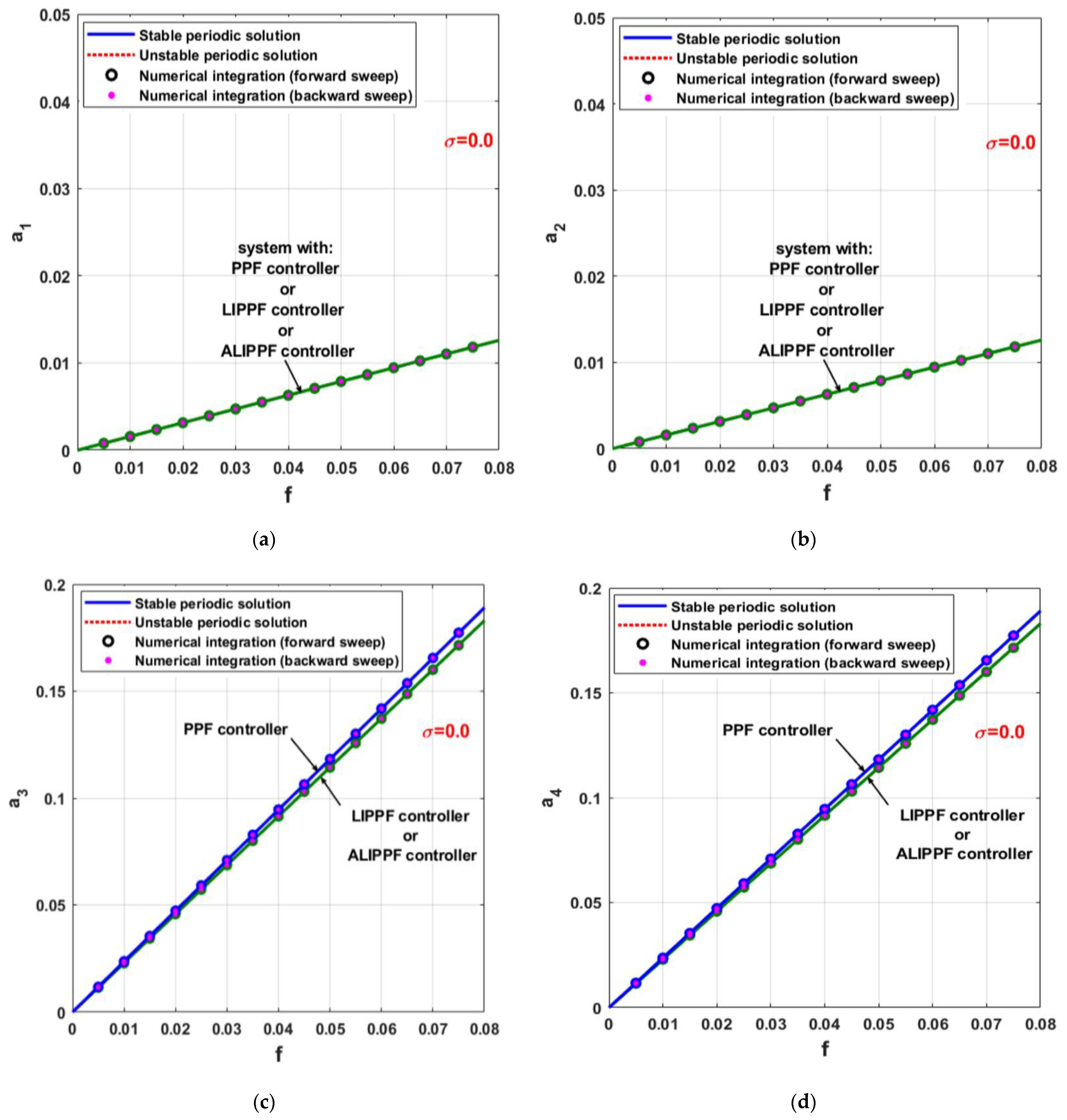
• The uncontrolled eight-pole electro-magnetic suspension system may respond as a linear system at the small rotor eccentricity ($f$) (i.e., $f<0.01$).
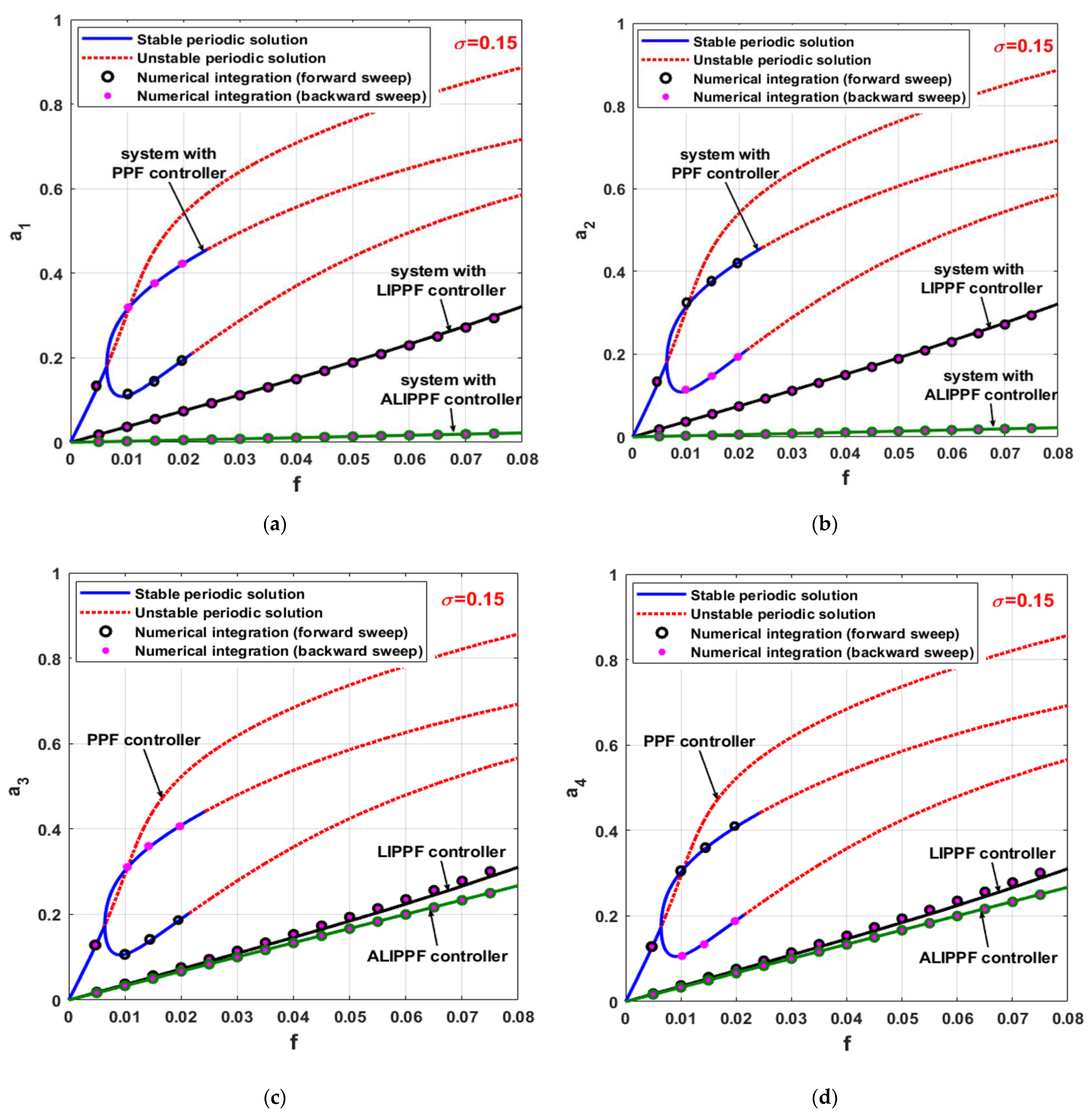
• At the large rotor eccentricity, the electro-magnetic suspension system may lose its stability to perform quasi-periodic or chaotic oscillations thanks to the complex bifurcation behaviors.
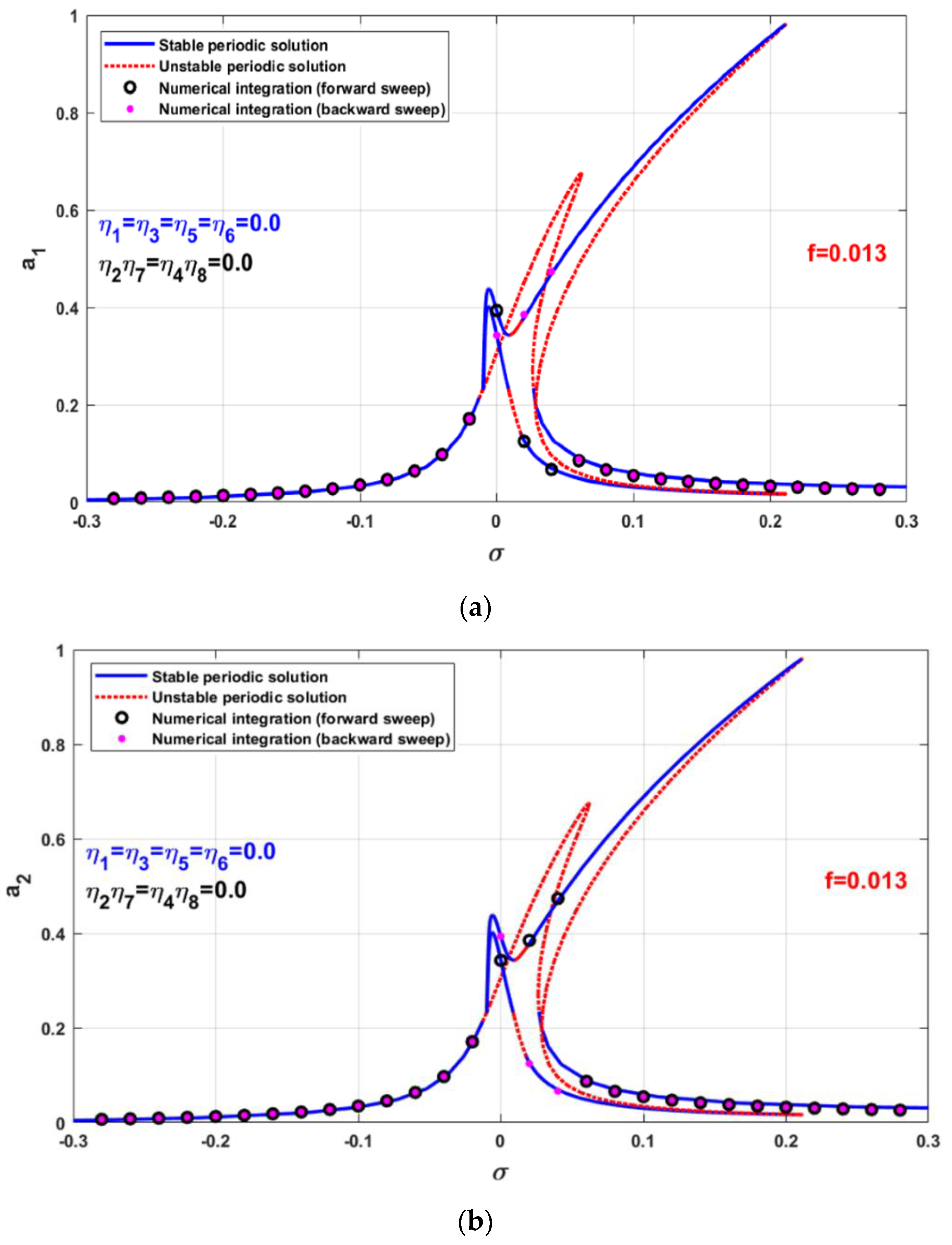
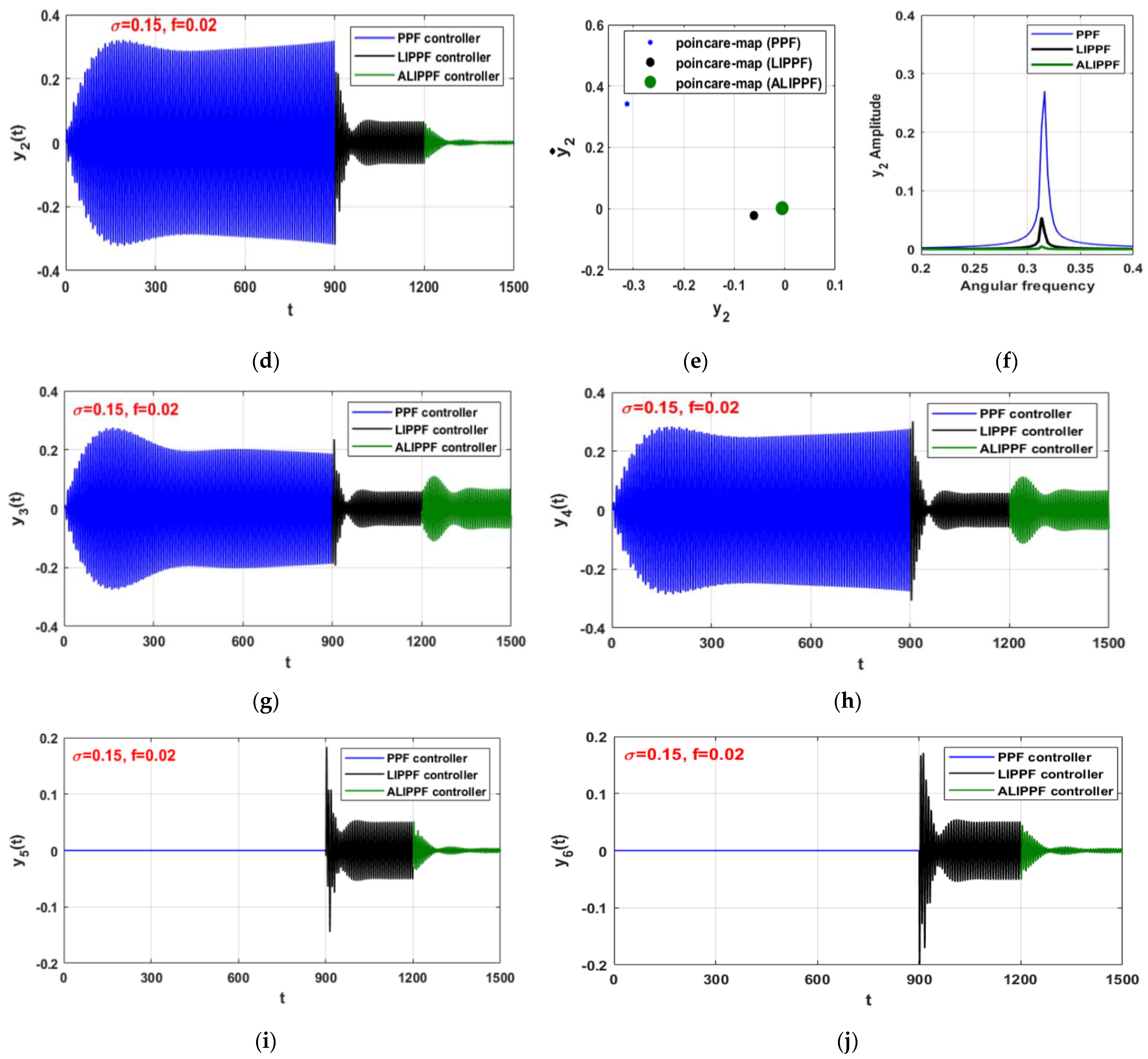
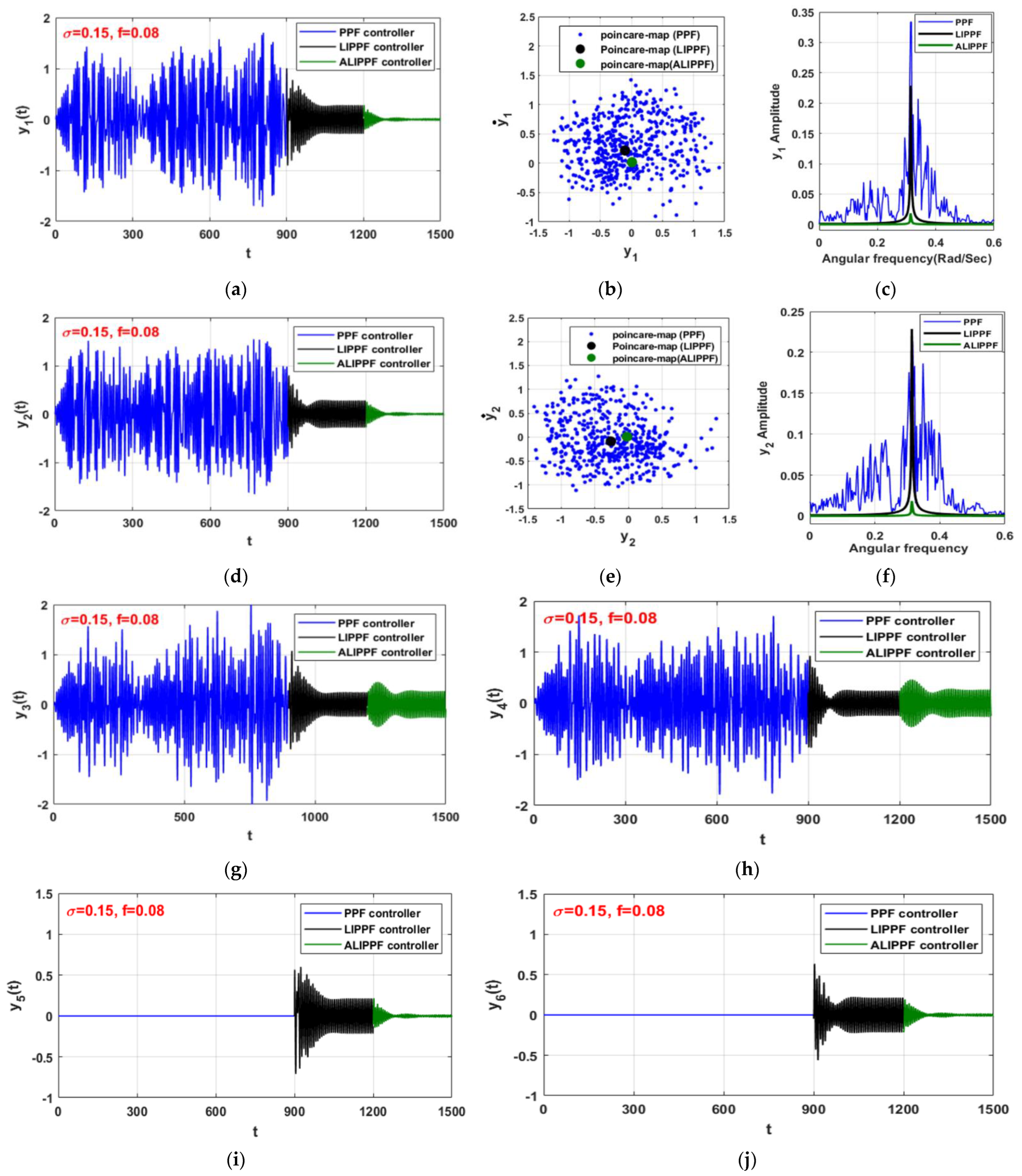
• Integrating the conventional PPF-controller into the electro-magnetic suspension system can eliminate the rotor vibration amplitudes at the perfect resonance conditions (i.e., $\sigma =0$). However, the PPF-controller can add more excessive vibratory energy to the rotor system rather than suppress it if the perfect resonance conditions have been lost.
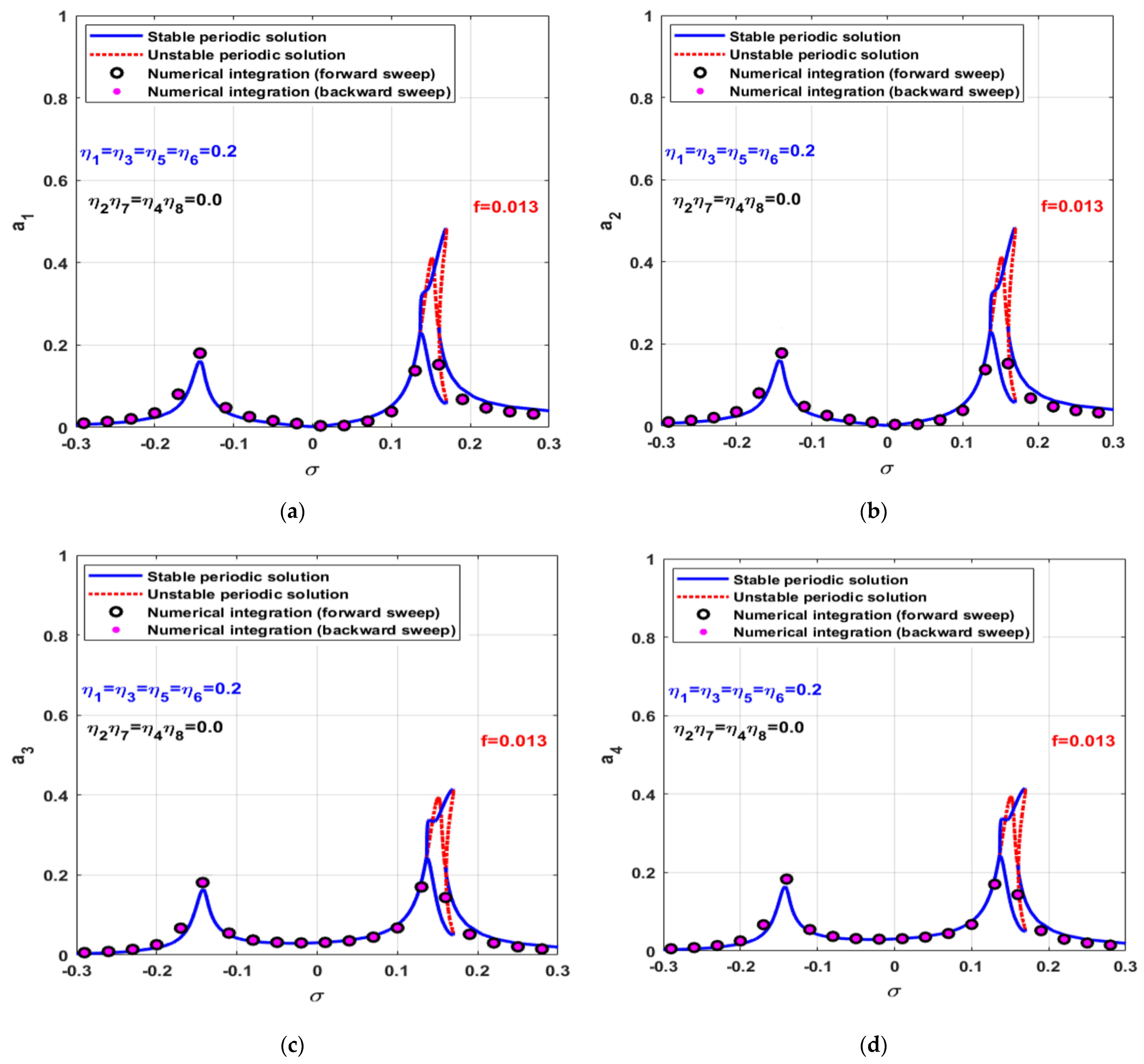
• The coupling of the LIR-controller to the eight-pole electromagnetic suspension system can eliminate the non-linear bifurcation and force the rotor to respond as a linear dynamical system. However, the controlled system may exhibit high oscillation at the perfect resonance conditions (i.e., $\sigma =0$).
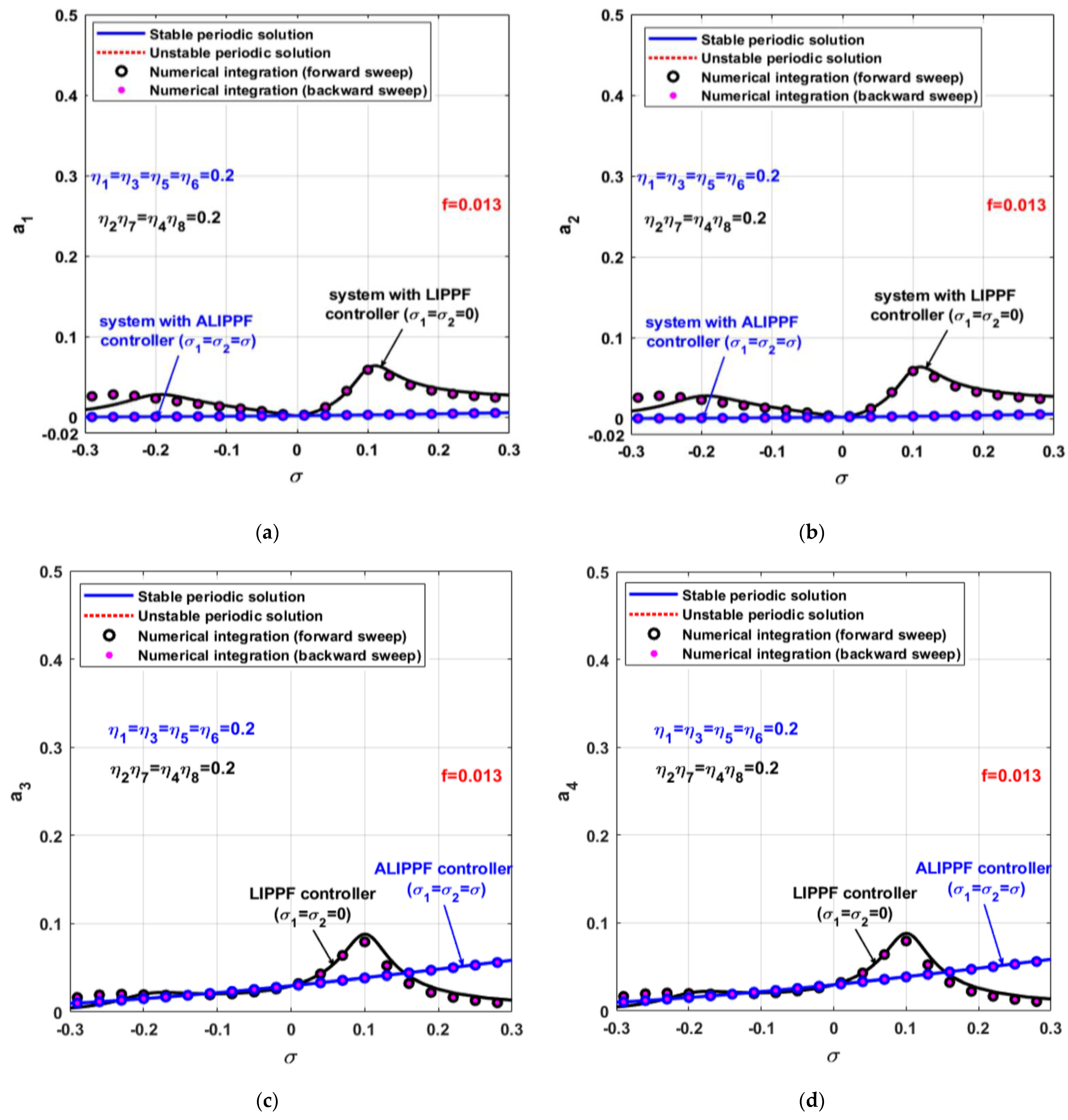
• The integration of the LIPPF-controller to the considered system can eliminate rotor oscillations at the perfect resonance conditions as well as suppress the non-linear vibrations to very small magnitudes if the resonance conditions have been lost.
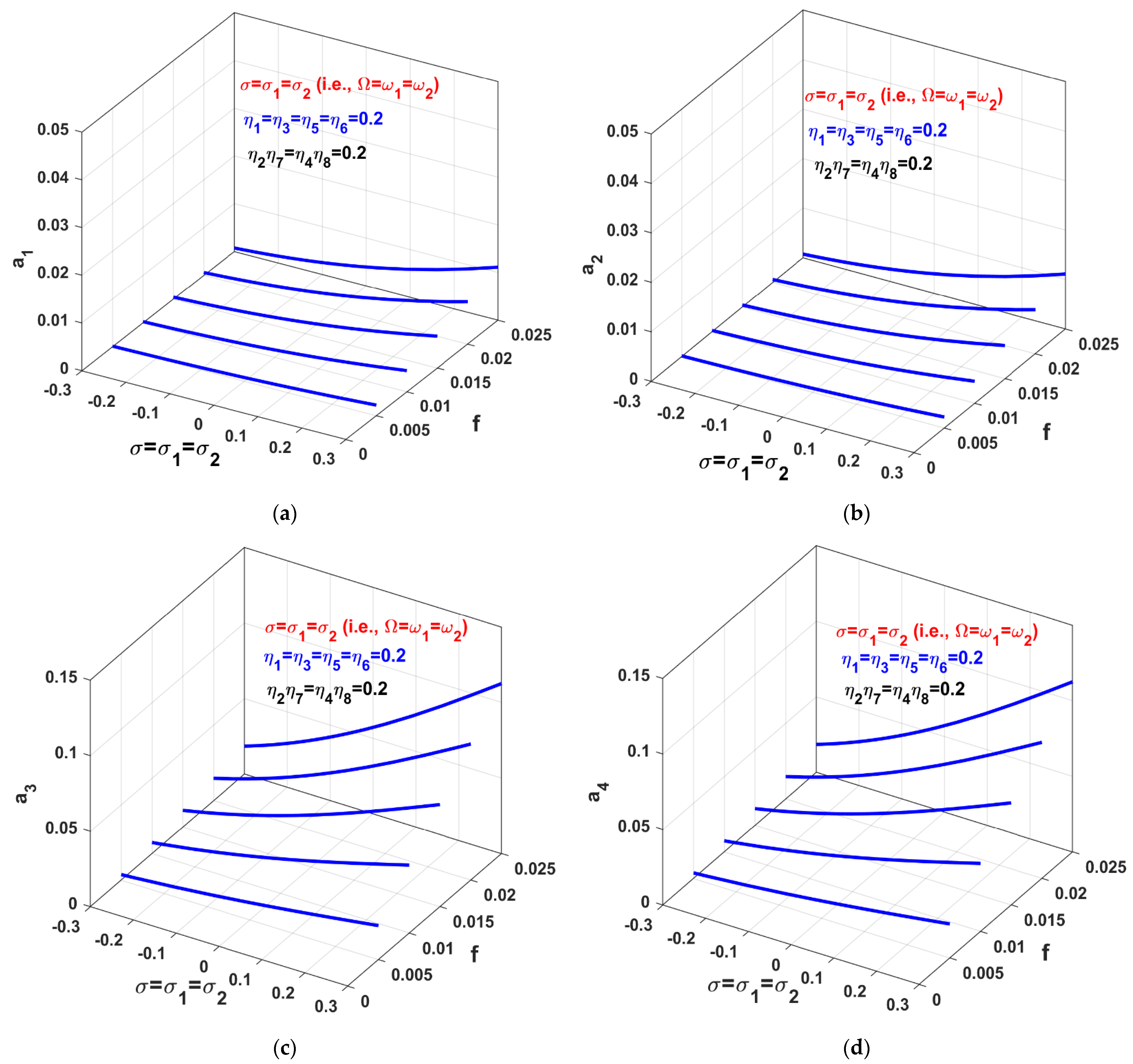
• The ALIPPF-controller (i.e., when setting ${\omega }_1={\omega }_2=\Omega$) can eliminate the undesired vibrations of the electro-magnetic suspension system to zero regardless of the angular speed and eccentricity of the rotating shaft.

References

1. Ji, J.C.; Yu, L.; Leung, A.Y.T. Bifurcation behavior of a rotor supported by active magnetic bearings. J. Sound Vib. 2000, 235, 133–151. [Google Scholar] [CrossRef]
2. Saeed, N.A.; Mahrous, E.; Awrejcewicz, J. Non-linear dynamics of the six-pole rotor-AMBs under two different control configurations. Non-Linear Dyn. 2020, 101, 2299–2323. [Google Scholar] [CrossRef]
3. Saeed, N.A.; Awwad, E.M.; El-Meligy, M.A.; Nasr, E.S.A. Radial versus Cartesian Control Strategies to Stabilize the Non-linear Whirling Motion of the Six-Pole Rotor-AMBs. IEEE Access 2020, 8, 138859–138883. [Google Scholar] [CrossRef]
4. Ji, J.C.; Hansen, C.H. Non-linear oscillations of a rotor in active magnetic bearings. J. Sound Vib. 2001, 240, 599–612. [Google Scholar] [CrossRef]
5. Ji, J.C.; Leung, A.Y.T. Non-linear oscillations of a rotor-magnetic bearing system under superharmonic resonance conditions. Int. J. Non-Linear Mech. 2003, 38, 829–835. [Google Scholar] [CrossRef]
6. El-Shourbagy, S.M.; Saeed, N.A.; Kamel, M.; Raslan, K.R.; Abouel Nasr, E.; Awrejcewicz, J. On the Performance of a Non-linear Position-Velocity Controller to Stabilize Rotor-Active Magnetic-Bearings System. Symmetry 2021, 13, 2069. [Google Scholar] [CrossRef]
7. Saeed, N.A.; Mahrous, E.; Abouel Nasr, E.; Awrejcewicz, J. Non-linear dynamics and motion bifurcations of the rotor active magnetic bearings system with a new control scheme and rub-impact force. Symmetry 2021, 13, 1502. [Google Scholar] [CrossRef]
8. Zhang, W.; Zhan, X.P. Periodic and chaotic motions of a rotor-active magnetic bearing with quadratic and cubic terms and time-varying stiffness. Non-Linear Dyn. 2005, 41, 331–359. [Google Scholar] [CrossRef]
9. Zhang, W.; Yao, M.H.; Zhan, X.P. Multi-pulse chaotic motions of a rotor-active magnetic bearing system with time-varying stiffness. Chaos Solitons Fractals 2006, 27, 175–186. [Google Scholar] [CrossRef]
10. Zhang, W.; Zu, J.W.; Wang, F.X. Global bifurcations and chaos for a rotor-active magnetic bearing system with time-varying stiffness. Chaos Solitons Fractals 2008, 35, 586–608. [Google Scholar] [CrossRef]
11. Zhang, W.; Zu, J.W. Transient and steady non-linear responses for a rotor-active magnetic bearings system with time-varying stiffness. Chaos Solitons Fractals 2008, 38, 1152–1167. [Google Scholar] [CrossRef]
12. Li, J.; Tian, Y.; Zhang, W.; Miao, S.F. Bifurcation of multiple limit cycles for a rotor-active magnetic bearings system with time-varying stiffness. Int. J. Bifurc. Chaos 2008, 18, 755–778. [Google Scholar] [CrossRef]
13. Li, J.; Tian, Y.; Zhang, W. Investigation of relation between singular points and number of limit cycles for a rotor–AMBs system. Chaos Solitons Fractals 2009, 39, 1627–1640. [Google Scholar] [CrossRef]
14. El-Shourbagy, S.M.; Saeed, N.A.; Kamel, M.; Raslan, K.R.; Aboudaif, M.K.; Awrejcewicz, J. Control Performance, Stability Conditions, and Bifurcation Analysis of the Twelve-Pole Active Magnetic Bearings System. Appl. Sci. 2021, 11, 10839. [Google Scholar] [CrossRef]
15. Saeed, N.A.; Kandil, A. Two different control strategies for 16-pole rotor active magnetic bearings system with constant stiffness coefficients. Appl. Math. Model. 2021, 92, 1–22. [Google Scholar] [CrossRef]
16. Wu, R.; Zhang, W.; Yao, M.H. Non-linear vibration of a rotor-active magnetic bearing system with 16-pole legs. In Proceedings of the International Design Engineering Technical Conferences and Computers and Information in Engineering Conference, Cleveland, OH, USA, 6–9 August 2017. [Google Scholar] [CrossRef]
17. Wu, R.; Zhang, W.; Yao, M.H. Analysis of non-linear dynamics of a rotor-active magnetic bearing system with 16-pole legs. In Proceedings of the International Design Engineering Technical Conferences and Computers and Information in Engineering Conference, Cleveland, OH, USA, 6–9 August 2017. [Google Scholar] [CrossRef]
18. Wu, R.Q.; Zhang, W.; Yao, M.H. Non-linear dynamics near resonances of a rotor-active magnetic bearings system with 16-pole legs and time varying stiffness. Mech. Syst. Signal Process. 2018, 100, 113–134. [Google Scholar] [CrossRef]
19. Zhang, W.; Wu, R.Q.; Siriguleng, B. Non-linear Vibrations of a Rotor-Active Magnetic Bearing System with 16-Pole Legs and Two Degrees of Freedom. Shock Vib. 2020, 2020, 5282904. [Google Scholar] [CrossRef]
20. Ma, W.S.; Zhang, W.; Zhang, Y.F. Stability and multi-pulse jumping chaotic vibrations of a rotor-active magnetic bearing system with 16-pole legs under mechanical-electric-electro-magnetic excitations. Eur. J. Mech. A/Solids 2021, 85, 104120. [Google Scholar] [CrossRef]
21. Ishida, Y.; Inoue, T. Vibration suppression of non-linear rotor systems using a dynamic damper. J. Vib. Control 2007, 13, 1127–1143. [Google Scholar] [CrossRef]
22. Saeed, N.A.; Awwad, E.M.; El-Meligy, M.A.; Nasr, E.S.A. Sensitivity analysis and vibration control of asymmetric non-linear rotating shaft system utilizing 4-pole AMBs as an actuator. Eur. J. Mech. A/Solids 2021, 86, 104145. [Google Scholar] [CrossRef]
23. Saeed, N.A.; Eissa, M. Bifurcation analysis of a transversely cracked non-linear Jeffcott rotor system at different resonance cases. Int. J. Acoust. Vib. 2019, 24, 284–302. [Google Scholar] [CrossRef]
24. Saeed, N.A.; Awwad, E.M.; El-Meligy, M.A.; Nasr, E.S.A. Analysis of the rub-impact forces between a controlled non-linear rotating shaft system and the electromagnet pole legs. Appl. Math. Model. 2021, 93, 792–810. [Google Scholar] [CrossRef]
25. Shan, J.; Liu, H.; Sun, D. Slewing and vibration control of a single-link flexible manipulator by positive position feedback (PPF). Mechatronics 2005, 15, 487–503. [Google Scholar] [CrossRef]
26. Ahmed, B.; Pota, H.R. Dynamic compensation for control of a rotary wing UAV using positive position feedback. J. Intell. Robot. Syst. 2011, 61, 43–56. [Google Scholar] [CrossRef] [Green Version]
27. Warminski, J.; Bochenski, M.; Jarzyna, W.; Filipek, P.; Augustyinak, M. Active suppression of non-linear composite beam vibrations by selected control algorithms. Commun. Non-Linear Sci. Numer. Simul. 2011, 16, 2237–2248. [Google Scholar] [CrossRef]
28. El-Ganaini, W.A.; Saeed, N.A.; Eissa, M. Positive position feedback (PPF) controller for suppression of nonlinear system vibration. Nonlinear Dyn. 2013, 72, 517–537. [Google Scholar] [CrossRef]
29. Saeed, N.A.; Kandil, A. Lateral vibration control and stabilization of the quasiperiodic oscillations for rotor-active magnetic bearings system. Nonlinear Dyn. 2019, 98, 1191–1218. [Google Scholar] [CrossRef]
30. Diaz, I.M.; Pereira, E.; Reynolds, P. Integral resonant control scheme for cancelling human-induced vibrations in light-weight pedestrian structures. Struct. Control Health Monit. 2012, 19, 55–69. [Google Scholar] [CrossRef]
31. Al-Mamun, A.; Keikha, E.; Bhatia, C.S.; Lee, T.H. Integral resonant control for suppression of resonance in piezoelectric micro-actuator used in precision servomechanism. Mechatronics 2013, 23, 1–9. [Google Scholar] [CrossRef]
32. Omidi, E.; Mahmoodi, S.N. Non-linear integral resonant controller for vibration reduction in non-linear systems. Acta Mech. Sin. 2016, 32, 925–934. [Google Scholar] [CrossRef]
33. MacLean, J.D.J.; Sumeet, S.A. A modified linear integral resonant controller for suppressing jump phenomenon and hysteresis in micro-cantilever beam structures. J. Sound Vib. 2020, 480, 115365. [Google Scholar] [CrossRef]
34. Omidi, E.; Mahmoodi, S.N. Sensitivity analysis of the Non-linear Integral Positive Position Feedback and Integral Resonant controllers on vibration suppression of non-linear oscillatory systems. Commun. Non-Linear Sci. Numer. Simul. 2015, 22, 149–166. [Google Scholar] [CrossRef]
35. Omidi, E.; Mahmoodi, S.N. Non-linear vibration suppression of flexible structures using non-linear modified positive position feedback approach. Non-Linear Dyn. 2015, 79, 835–849. [Google Scholar] [CrossRef]
36. Saeed, N.A.; Awrejcewicz, J.; Alkashif, M.A.; Mohamed, M.S. 2D and 3D Visualization for the Static Bifurcations and Nonlinear Oscillations of a Self-Excited System with Time-Delayed Controller. Symmetry 2022, 14, 621. [Google Scholar] [CrossRef]
37. Saeed, N.A.; Moatimid, G.M.; Elsabaa, F.M.; Ellabban, Y.Y.; Elagan, S.K.; Mohamed, M.S. Time-Delayed Non-linear Integral Resonant Controller to Eliminate the Non-linear Oscillations of a Parametrically Excited System. IEEE Access 2021, 9, 74836–74854. [Google Scholar] [CrossRef]
38. Saeed, N.A.; Mohamed, M.S.; Elagan, S.K.; Awrejcewicz, J. Integral Resonant Controller to Suppress the Non-linear Oscillations of a Two-Degree-of-Freedom Rotor Active Magnetic Bearing System. Processes 2022, 10, 271. [Google Scholar] [CrossRef]
39. Nayfeh, A.H.; Mook, D.T. Non-Linear Oscillations; Wiley: New York, NY, USA, 1995. [Google Scholar]
40. Nayfeh, A.H. Resolving Controversies in the Application of the Method of Multiple Scales and the Generalized Method of Averaging. Non-Linear Dyn. 2005, 40, 61–102. [Google Scholar] [CrossRef]
41. De la Luz Sosa, J.; Olvera-Trejo, D.; Urbikain, G.; Martinez-Romero, O.; Elías-Zúñiga, A.; Lacalle, L.N.L.d. Uncharted Stable Peninsula for Multivariable Milling Tools by High-Order Homotopy Perturbation Method. Appl. Sci. 2020, 10, 7869. [Google Scholar] [CrossRef]
42. Puma-Araujo, S.D.; Olvera-Trejo, D.; Martínez-Romero, O.; Urbikain, G.; Elías-Zúñiga, A.; López de Lacalle, L.N. Semi-Active Magnetorheological Damper Device for Chatter Mitigation during Milling of Thin-Floor Components. Appl. Sci. 2020, 10, 5313. [Google Scholar] [CrossRef]
43. Urbikain, G.; Olvera, D.; López de Lacalle, L.N.; Beranoagirre, A.; Elías-Zuñiga, A. Prediction Methods and Experimental Techniques for Chatter Avoidance in Turning Systems: A Review. Appl. Sci. 2019, 9, 4718. [Google Scholar] [CrossRef] [Green Version]
44. Urbikain, G.; Olvera-Trejo, D.; López de Lacalle, L.N.; Elías-Zúñiga, A. Spindle speed variation technique in turning operations: Modeling and real implementation. J. Sound Vib. 2016, 383, 384–396. [Google Scholar] [CrossRef]
45. Urbikain, G.; Olvera-Trejo, D.; López de Lacalle, L.N.; Elías-Zúñiga, A. Stability and vibrational behaviour in turning processes with low rotational speeds. Int. J. Adv. Manuf. Technol. 2015, 80, 871–885. [Google Scholar] [CrossRef]
46. Ishida, Y.; Yamamoto, T. Linear and Non-Linear Rotordynamics: A Modern Treatment with Applications, 2nd ed.; Wiley-VCH Verlag GmbH & Co. KGaA: New York, NY, USA, 2012. [Google Scholar] [CrossRef]
47. Schweitzer, G.; Maslen, E.H. Magnetic Bearings: Theory, Design, and Application to Rotating Machinery; Springer: Berlin/Heidelberg, Germany, 2009. [Google Scholar] [CrossRef]
48. Slotine, J.-J.E.; Li, W. Applied Non-Linear Control; Prentice Hall: Englewood Cliffs, NJ, USA, 1991. [Google Scholar]
49. Yang, W.Y.; Cao, W.; Chung, T.; Morris, J. Applied Numerical Methods Using Matlab; John Wiley & Sons, Inc.: Hoboken, NJ, USA, 2005. [Google Scholar]
Figure 1. (a) The 3-D visualization of the eight-pole electro-magnetic suspension system, (b) schematic diagram of the eight-pole electro-magnetic suspension system when the rotor lies within its nominal position, (c) schematic diagram of the eight-pole electro-magnetic suspension system when the rotor makes displacements x 1 ( t ) and x 2 ( t ) in X 1 and X 2 directions, respectively.
Applsci 12 03902 g001
Figure 2. The schematic diagram shows the interconnection between the proposed LIPPF-controller and the electro-magnetic suspension system.
Applsci 12 03902 g002
Figure 3. Vibration amplitudes of the rotor system without the LIPPF-controller using σ as a bifurcation parameter when f = 0.001 ,   0.004 ,   0.007 ,   0.01 , and 0.013 : (a) vibration amplitude in X 1   direction and (b) vibration amplitude in X 2 direction.
Applsci 12 03902 g003
Figure 4. Vibration amplitudes of the rotor system and PPF-controller using σ as a bifurcation parameter when f = 0.005 ,   0.01 ,   0.015 ,   0.02 , and 0.025 : (a) vibration amplitude in X 1 direction, (b) vibration amplitude in X 2 direction, and (c,d) vibration amplitudes of the PPF-controller.
Applsci 12 03902 g004
Figure 5. Vibration amplitudes of the rotor system and LIPPF-controller using σ as a bifurcation parameter when f = 0.005 ,   0.01 ,   0.015 ,   0.02 , and 0.025 : (a) vibration amplitude in X 1 direction, (b) vibration amplitude in X 2 direction, and (c,d) vibration amplitudes of the LIPPF-controller.
Applsci 12 03902 g005
Figure 6. Vibration amplitudes of the rotor system and LIPPF-controller using σ as a bifurcation parameter at various values of σ 1 = σ 2 when f = 0.015 : (a) vibration amplitude in X 1 direction, (b) vibration amplitude in X 2 direction, and (c,d) vibration amplitudes of the LIPPF-controller.
Applsci 12 03902 g006
Figure 7. Vibration amplitudes of the rotor system and ALIPPF-controller using σ = σ 1 = σ 2 as a bifurcation parameter when f = 0.005 ,   0.01 ,   0.015 ,   0.02 , and 0.025 : (a) vibration amplitude in X 1 direction, (b) vibration amplitude in X 2 direction, and (c,d) vibration amplitudes of the LIPPF-controller.
Applsci 12 03902 g007
Figure 8. Vibration amplitudes of the rotor system without the LIPPF-controller using σ as a bifurcation parameter when f = 0.013 : (a) vibration amplitude in X 1 direction and (b) vibration amplitude in X 2 direction.
Applsci 12 03902 g008
Figure 9. Vibration amplitudes of the rotor system and PPF-controller using σ as a bifurcation parameter when f = 0.013 : (a) vibration amplitude in X 1 direction, (b) vibration amplitude in X 2 direction, and (c,d) vibration amplitudes of the PPF-controller.
Applsci 12 03902 g009
Figure 10. Vibration amplitudes of the rotor system, LIPPF-controller, and ALIPPF-controller when f = 0.013 : (a) vibration amplitude in X 1 direction, (b) vibration amplitude in X 2 direction, and (c,d) vibration amplitudes of the LIPPF-controller and ALIPPF-controller.
Applsci 12 03902 g010
Figure 11. Vibration amplitudes of the rotor system, PPF-controller, LIPPF-controller, and ALIPPF-controller using the rotor eccentricity f a bifurcation parameter when σ = 0 : (a) vibration amplitude in X 1 direction, (b) vibration amplitude in X 2 direction, and (c,d) vibration amplitudes of the PPF-controller, LIPPF-controller, and ALIPPF-controller.
Applsci 12 03902 g011
Figure 12. Vibration amplitudes of the rotor system, PPF-controller, LIPPF-controller, and ALIPPF-controller using the rotor eccentricity f a bifurcation parameter when σ = 0.15 : (a) vibration amplitude in X 1 direction, (b) vibration amplitude in X 2 direction, and (c,d) vibration amplitudes of the PPF-controller, LIPPF-controller, and ALIPPF-controller.
Applsci 12 03902 g012
Figure 13. Rotor electro-magnetic suspension time response, Poincare map, and the frequency spectrum with the PPF-controller, LIPPF-controller, and ALIPPF-controller at σ = 0.15 and f = 0.02 : (a,d) the temporal oscillations of the rotor system in X 1 and X 2 directions, (b,e) the corresponding Poincare map of the rotor system, (c,f) the corresponding frequency spectrum of the rotor, and (gj) the temporal oscillations of the controllers.
Applsci 12 03902 g013aApplsci 12 03902 g013b
Figure 14. Rotor electro-magnetic suspension time response, Poincare map, and the frequency spectrum with the PPF-controller, LIPPF-controller, and ALIPPF-controller at σ = 0.15 and f = 0.05 : (a,d) the temporal oscillations of the rotor system in X 1 and X 2 directions, (b,e) the corresponding Poincare map of the rotor system, (c,f) the corresponding frequency spectrum of the rotor, and (gj) the temporal oscillations of the controllers.
Applsci 12 03902 g014
Figure 15. Rotor electro-magnetic suspension time response, Poincare map, and the frequency spectrum with the PPF-controller, LIPPF-controller, and ALIPPF-controller at σ = 0.15 and f = 0.08 : (a,d) the temporal oscillations of the rotor system in X 1 and X 2 directions, (b,e) the corresponding Poincare map of the rotor system, (c,f) the corresponding frequency spectrum of the rotor, and (gj) the temporal oscillations of the controllers.
Applsci 12 03902 g015
Publisher’s Note: MDPI stays neutral with regard to jurisdictional claims in published maps and institutional affiliations.