Article

Dynamic Analysis of a Wiper Blade in Consideration of Attack Angle and Clarification of the Jumping Phenomenon

1
Mechanical Systems Laboratory, Degree Programs in Systems and Information Engineering, University of Tsukuba, Tsukuba 305-8573, Japan
2
MITSUBA Co., Ltd., Kiryu 376-0013, Japan
*
Author to whom correspondence should be addressed.
Appl. Sci. 2022, 12(9), 4112; https://doi.org/10.3390/app12094112
Submission received: 14 March 2022 / Revised: 13 April 2022 / Accepted: 15 April 2022 / Published: 19 April 2022
(This article belongs to the Special Issue Nonlinear Vibrations)

Abstract

:
Automobile windshields are typically curved, creating an oblique angle of attack between the wiper blade and the windshield. This attack angle means that the wiper may jump off the windshield while wiping, causing a chattering noise and preventing the rainwater from being fully wiped off the windshield. Thus, it is important to examine the dynamics of the wiper blade under friction. In this study, the relationship between the attack angle and the jumping phenomenon is clarified through dynamic analysis. We introduce an analytical two-link model corresponding to an actual wiper blade that considers the exchange of dynamic and static friction between the windshield and the blade. The dynamic friction is assumed to be negatively correlated with the relative velocity, and the static friction is described by a set-valued function. As the motion transitions from the stick state to the slip state, the equation to be solved changes. Hence, the initial condition after a transition must agree with the final condition before the transition. Because the governing equations are nonlinear and the solution is highly dependent on the initial condition, the transition time and corresponding state variables are vital. The slack variable method is used to obtain the exact transition time and initial conditions. The sign of the normal force acting on the blade from the windshield determines the occurrence of the jump phenomenon. A larger attack angle makes the jump phenomenon more likely. However, the jump phenomenon does not occur when the motion of the blade reverses. Experimental observations support the theoretical description of the wiper blade.

1. Introduction

To ensure excellent aerodynamic performance and aesthetics, automobile windshields are generally constructed to have some integral curvature. Thus, an angle is generated between the symmetry plane of the wiper blade and the normal vector of the windshield surface. This is defined as the attack angle. The presence of the attack angle means that the wiper blade may jump away from the windshield during the wiping process, which causes a chattering noise and incomplete wiping. These issues negatively affect the driving experience and pose a safety hazard. In developing the optimal wiper blade design that does not suffer from the jumping phenomenon, it is essential to understand the dynamics of the wiper blade in consideration of the attack angle.
Several studies have analyzed the jumping phenomenon and chatter noise of wiper blades. Grenouillat et al. [1] conducted experiments to determine the range of pressure that keeps the wiper blade in contact with the wiping surface and the attack angles at which chatter noise occurs. A four-degree-of-freedom model including the displacement of the holder in the transverse and longitudinal directions was then developed and analyzed. By analyzing the stability of the model with respect to the pressure under different attack angles, the conditions for the unstable motion of the wiper blade were derived. The theoretically obtained results were found to be in good agreement with the experimental data. Awang et al. [2] built a finite element model of the whole wiper system, including the arm and levers, to analyze the chatter noise and vibration generated by the wiper blade. They used this model to perform complex eigenvalue analysis and achieved good agreement with experimental modal analysis and vibration measurements. Furthermore, they proposed several improved wiper profiles. Lancioni et al. [3] employed numerical analysis to elucidate how the attack angle affects the wiper blade to produce the jumping phenomenon. In addition to the slip state and stick state, the free flight state after jumping was analyzed. They found that a chattering of about 100 Hz was produced, indicating that this is a complex vibration that mixes the above three different states of motion. Their study also considered different types of friction and the change of rotational stiffness created by the contact between the lip and wiper head. However, the wiper blade was only modeled with one link, and no experimental verification was performed. Okura et al. [4] developed a theoretical model of a wiper with an arm and blade to analyze the dynamics of the wiper system. The gradient of the coefficient of dynamic friction with respect to velocity was considered in the model, as was the attack angle. The condition whereby the wiper blade jumps away from the windshield was analyzed independently, and the equation of motion was determined for various conditions. Although this study considered the contact between the shoulder and the head, it was assumed that the angle of the link would not change after the contact, and the stiffness was fixed. Unfortunately, the results obtained from the theoretical analysis were not supported by experimental data. Zolfagharian et al. [5] used a control method combining particle swarm optimization with an input-shaping controller to suppress the wiper blade noise produced by the horizontal stick–slip motion and the vertical jump phenomenon. Using this method, the timing of the input control signal could be adjusted optimally. Experiments found that the noise was effectively suppressed compared with the case without control. However, this study only provided a control method; there was no detailed dynamic analysis to clarify the mechanism whereby various behaviors were produced.
In studying the dynamics of wiper blades, the characterization of the friction between the wiper blade and the windshield is an important factor that cannot be ignored. Koenen et al. [6] performed experiments to test how friction affects the wiper dynamics under different motion conditions. They found that the coefficient of dynamic friction decreases with increasing temperature in dry conditions. In wet conditions, the coefficient of dynamic friction is large in the boundary regime with an almost-zero wiping velocity and becomes small in the hydrodynamic regime corresponding to faster wiping velocities. Between these two regimes, i.e., the mixed lubrication regime, the coefficient of dynamic friction decreases as the velocity increases. This relationship follows the Stribeck curve [7]. When water evaporates from the wiping surface, the glass becomes tacky. Under such conditions, the coefficient of dynamic friction is greater than in dry conditions. Nakano [8] used a simple one-degree-of-freedom model to analyze the mechanism of stick–slip motion under the influence of Coulomb friction. It was demonstrated that the difference between dynamic friction and static friction is the fundamental cause of stick–slip motion. Nakano concluded that the generation of this motion is related to the relative velocity, normal load, stiffness, and damping of the system. Bódai et al. [9] tested how the normal load and wiping velocity affect the coefficient of friction between the wiper and the glass. A special glass cylinder and wiper device were built to allow the behavior of friction in the entire wiper system to be studied. Furthermore, a mathematical model was developed to interpret the experimental results qualitatively. In their experiments in wet conditions, they found that the friction coefficient decreased with increasing normal load and wiping velocity. Le Rouzic et al. [10] used a one-degree-of-freedom spring–mass damper system under the influence of the Stribeck law to clarify the unstable velocity region in which the equilibrium state becomes unstable through a Hopf bifurcation leading to a cycle solution, i.e., self-excited oscillation. A series of experiments showed that the coefficient of dynamic friction and the relative velocity follow Stribeck curves. The wiping noise was found to be caused by self-excited vibration as a result of friction. However, the analytical model developed from the theory did not consist of a wiper head and links. Reddyhoff et al. [11] analyzed the vibration mechanism of the wiper generated by friction. Their experiments indicated that the wiper blade generates two frequency components of vibration during sliding. Finite element analysis clarified that these two frequency components match the eigenfrequencies of the first two bending modes of the blade. It was also shown that water has the effect of adding mass to the system, thus affecting the vibration frequency. As a result, they proposed several solutions for reducing the wiper noise. Unno et al. [12] investigated the dynamics around the wiper reversal point through numerical analysis and experiments. Dynamic and static friction were modeled separately, and different equations were solved numerically for the slip and stick states. To ensure the correctness of the numerical analysis of the nonlinear system, the exact transition times of the different states were derived using the slack variable method. Further experiments were conducted to verify the theoretical analysis. However, the effects of the attack angle and the nonlinear rotation stiffness on the system dynamics were not considered in this study, despite the attack angle being an important aspect in the wiper blade dynamics.
In the study of the tribology between rubber and glass, the change in the coefficient of dynamic friction under wet conditions is particularly critical. Deleau et al. [13] investigated the tribological behavior of the contact between the rubber blade and the windshield. On a wet windshield, the rubber blade has the same actual contact area as on a dry windshield under extremely slow velocity. However, as the sliding velocity increases, the dry area gradually decreases, and a thin film of water can be formed. The lubrication effect of the thin film of water in between the rubber blade and windshield leads to a reduction in the coefficient of dynamic friction. Bódai et al. [14] clarified that the film arises because the pressure of the fluid gradually increases as the sliding velocity increases. Due to the presence of the film, the friction is mainly controlled by the fluid film friction. Thus, the friction coefficient is significantly reduced. However, due to the low viscosity of water, the reduction of the friction coefficient at low sliding velocity cannot be explained by the hydrodynamic effect.
Several studies have taken the attack angle into account. Chevennement-Roux et al. [15] developed a finite element model considering the attack angle to analyze the dynamics of the wiper system. The stability of the system was analyzed for different values of the normal pressure and attack angle. The validity of this model was then verified through a series of experiments. Min et al. [16] built an experimental setup to simulate the waves on the windshield. The waves have the effect of changing the contact angle of the wiper blade, which corresponds to the so-called attack angle effect. As the liquid on the windshield is removed by the wipers, the coefficient of dynamic friction becomes greater than 1. The waviness changes the wiping velocity of the wiper blade and the coefficient of dynamic friction, leading to noise.
In recent years, there have been many studies about wiper blades from different perspectives. Mohamad et al. [17] considered many factors that influence the dynamic behavior and characteristics of rubber wiper blade performance. These factors include the different types of wipers, environment conditions such as humidity, temperature, and air friction, as well as the stiffness increases of the used wiper blades. This study experimentally illustrated how these factors affect the dynamic behavior and characteristics of rubber wiper blade performance in great detail. Lee et al. [18] compared the wiper blade before use with the wiper blade after more than one year of use by structural analysis. The changes of the contact distribution and wiping angle were investigated to assess the mechanical properties and shape changes of the wiper blade due to prolonged use. Three main factors affecting the cross-section of the wiper blade were found. As a result, the design direction of the cross-sectional shape of a wiper blade was predicted. Chen et al. [19] solved the theoretical problem of the vibration of rubber wiper blades on the convex windshield. The three-dimensional vibration problem from the elasticity perspective was considered. Two classes of vibration frequencies corresponding to two types of deformation were found by the theoretical analysis. Then, two mathematical formulas for the vibration problem of the rubber wiper blade on a convex windshield were obtained. The theoretical predictions were in good agreement with the experimental results.
In the present study, all of the above-mentioned factors are considered in analyzing the dynamics of the wiper blade. These factors include the attack angle, independent dynamic and static friction models, the lubrication effect of the thin film of water, and the change in rotation stiffness brought about by the shoulder–head contact. We first introduce a two-degree-of-freedom analytical model for the wiper blade. Dynamic friction is considered to be negatively related to the relative velocity of the motion, and static friction is considered to be a set-valued function that keeps the system in equilibrium. Unlike the case where the attack angle is not considered, the normal force cannot be obtained independently, because the friction force affects the normal force. A simulation algorithm was established based on the relevant equations. In the numerical simulations, we used different equations of motion to solve the corresponding motion states. As the governing equations in each state are nonlinear, the initial condition has a significant effect on the simulation result. To ensure the accuracy of the result, we used the slack variable method to determine the exact time at which the transition occurs between the different states. The purpose of this study is to analyze the dynamics of the wiper blade in the range where the normal force is positive, i.e., until the jump phenomenon occurs, and to detect the state of the wiper blade at this point. Through numerical simulations with different values of the attack angle, it is shown that a large attack angle makes the jumping phenomenon more likely to occur. The configuration of the blades required to produce the jump is theoretically determined. We also conduct experiments using a real wiper blade. The experimental results are in qualitatively good agreement with those from our theoretical system.

2. Analytical Two-Link Model and Equations of Motion

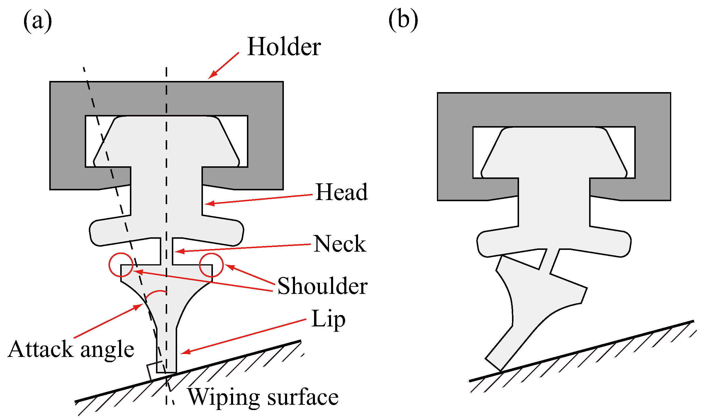
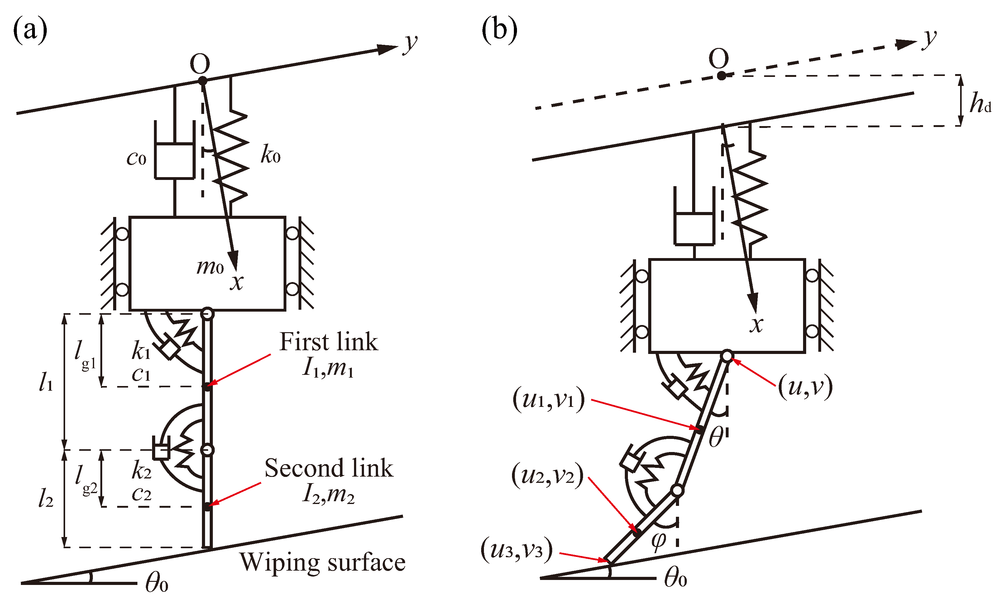
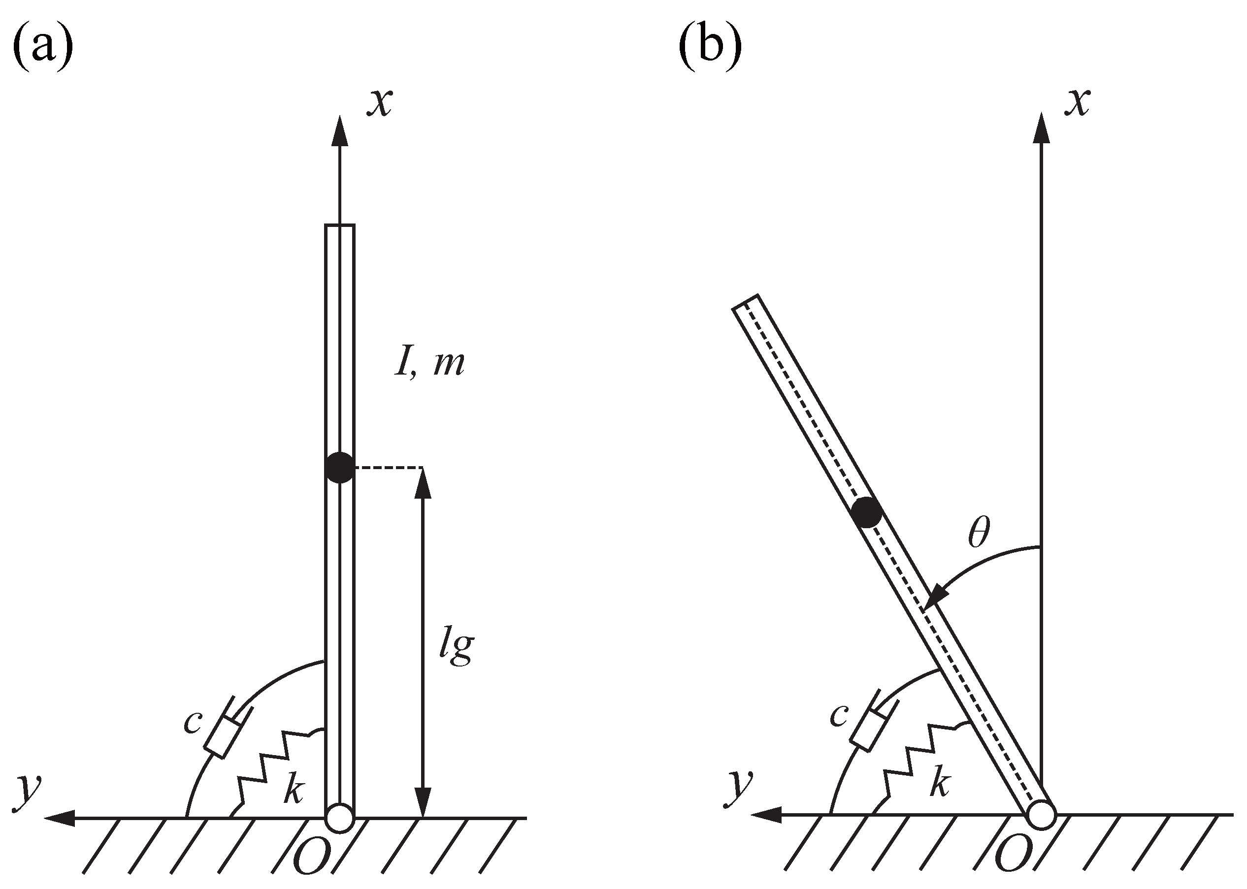
2.1. Analytical Two-Link Model

As shown in Figure 1, a wiper blade consists of a head, neck, and lip. The head is clamped by the holder so that the wiper blade can be driven by the holder. In general, the thickness of the wiper blade below the head is not uniform. As in the figure, the thickness of the lip gradually decreases from top to bottom below the narrow neck. The shoulder is formed at the very top of the lip. The contact between the shoulder and the head leads to an increase in rotation stiffness, and this effect is taken into account when we model the wiper blade. The wiping surface corresponding to the windshield is angled with respect to the horizontal surface. The angle generated between the center line of the wiper blade and the normal vector of the wiping surface is defined as the attack angle.
The two-link model of the wiper blade is shown in Figure 2. The first and second links (from top to bottom) correspond to the neck and lip, respectively. Their total length and the distance from the top to the center of gravity are indicated in the figure. The displacement of the head is limited in the horizontal direction by the holder, but it can move freely in the vertical direction. The mass, rotational inertia, stiffness, and damping of each component are also shown in the figure.
The origin is set at the uppermost position of the entire model when both links are pointing vertically downward and the head spring k 0 is at its original length. The x- and y-directions are perpendicular and parallel to the wiping surface, respectively; the x-axis is inclined from the vertical direction at θ 0 . To apply the normal load to the wiper blade, the spring k 0 can be compressed by a length of h d . The distance from the origin to the wiping surface is constant, so given the length h d , the position relationship of the entire model can be determined by the angles of the two links, θ and φ . Thus, this is a two-degree-of-freedom model in which the independent variables are the two link angles θ and φ . Our purpose is to clarify the characteristic dynamics under the transition between the dynamic and static friction of the wiper blade. We think that a simplified essential model with the smallest possible number of parameters is important to find the essential parameters governing the dynamics under the transition between dynamic and static frictions. The calculation results for the simple analytical model develop the physical understanding of the behavior of the wiper blade depending on the system parameters.
As mentioned above, the rotation stiffness of the first link increases when the shoulder contacts the head. To take this effect into account, the restoring moment of the first link M k 1 is given as follows:
M k 1 = k 12 θ + θ 0 k 12 k 11 θ c , θ + θ 0 < θ c k 11 θ + θ 0 , θ c θ + θ 0 θ c k 12 θ + θ 0 + k 12 k 11 θ c , θ + θ 0 > θ c .
The parameter k 11 represents the rotational stiffness of the first link without shoulder–head contact, and k 12 represents the rotational stiffness of the first link with shoulder–head contact. The parameter θ c represents the angle of the first link when contact between the shoulder and the head occurs.
The relationship between θ + θ 0 and M k 1 is illustrated in Figure 3. When the absolute value of the sum of the attack angle and the angle of the first link does not exceed θ c , i.e., the shoulder does not contact the head, the rotational stiffness of the first link is k 11 . The restoring moment varies within a narrow range. However, when the absolute value of the sum of the attack angle and the angle of the first link is greater than θ c , i.e., the shoulder contacts the head, the rotational stiffness of the first link becomes k 12 , which is much greater than k 11 . In this condition, the restoring moment changes from the maximum value in the non-contact case, and the rate of change with respect to the angle will increase.

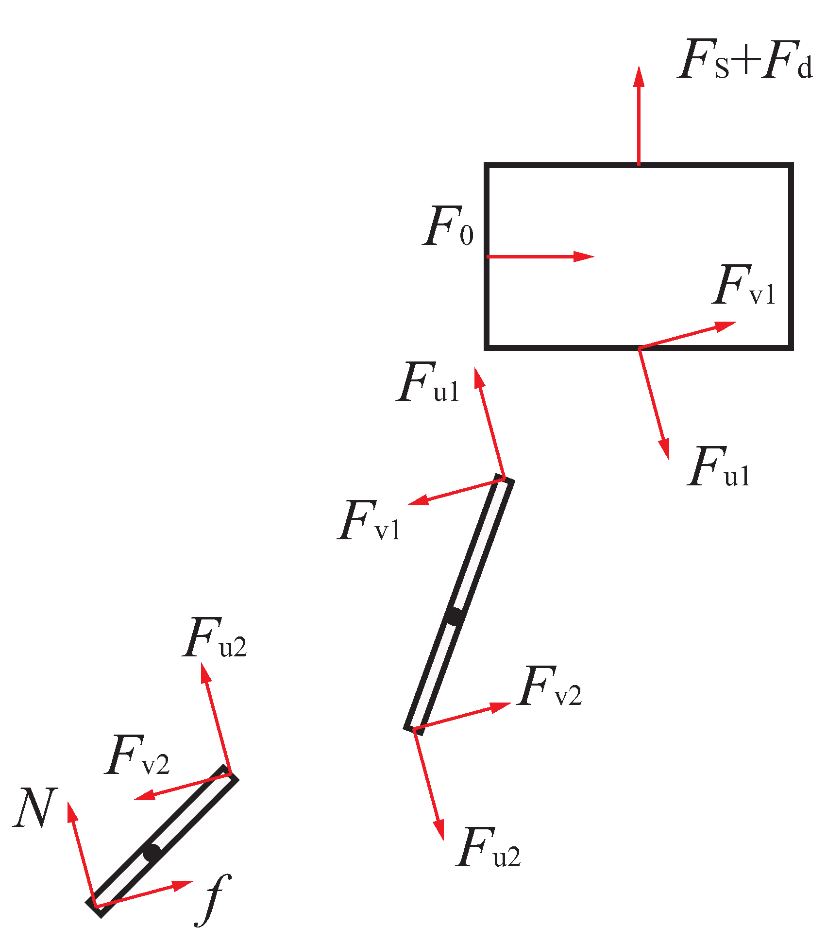
2.2. Equations of Motion of the Model

From the model, we can obtain the following governing equations of motion (a detailed derivation is given in Appendix A).
d 2 θ d t 2 m 0 + m 1 l 1 sin θ cos θ 0 + m 1 l g 1 sin ( θ + θ 0 ) + m 2 l 1 tan θ 0 cos ( θ + θ 0 ) + d 2 φ d t 2 m 0 + m 1 + m 2 l 2 sin φ cos θ 0 + m 2 l g 2 sin ( φ + θ 0 ) = d θ d t 2 m 0 + m 1 l 1 cos θ cos θ 0 m 1 l g 1 cos ( θ + θ 0 ) + m 2 l 1 tan θ 0 sin ( θ + θ 0 ) + d φ d t 2 m 0 + m 1 + m 2 l 2 cos φ cos θ 0 m 2 l g 2 cos ( φ + θ 0 ) + k 0 l 1 1 cos θ cos θ 0 + l 2 1 cos φ cos θ 0 h d + c 0 d θ d t l 1 sin θ cos θ 0 + d φ d t l 2 sin φ cos θ 0 + N cos θ 0 + f sin θ 0 m 0 + m 1 + m 2 a ω 2 sin θ 0 cos ω t ,
d 2 θ d t 2 m 1 l 1 l g 1 sin θ cos θ 0 sin θ + θ 0 + m 2 l 1 2 cos θ cos θ 0 cos θ + θ 0 + m 1 l g 1 2 + I 1 + d 2 φ d t 2 m 2 l 1 l g 1 cos φ θ m 1 l g 1 + m 2 l 1 l 2 sin φ sin θ + θ 0 cos θ 0 = d θ d t 2 m 1 l g 1 + m 2 l 1 l 1 cos θ sin θ + θ 0 cos θ 0 + d φ d t 2 m 1 l g 1 + m 2 l 1 l 2 cos φ sin θ + θ 0 cos θ 0 + m 2 l 1 l g 2 sin φ θ + M k 1 c 1 d θ d t + k 2 φ θ + c 2 d φ d t d θ d t + N l 1 sin θ + f l 1 cos θ m 1 l g 1 + m 2 l 1 a ω 2 cos θ cos ω t ,
d 2 θ d t 2 m 2 l 1 l g 2 cos φ cos θ 0 cos θ + θ 0 + d 2 φ d t 2 m 2 l 2 l g 2 sin φ cos θ 0 sin φ + θ 0 + m 2 l g 2 2 + I 2 = d θ d t 2 m 2 l 1 l g 2 cos φ sin θ + θ 0 cos θ 0 + d φ d t 2 m 2 l 2 l g 2 cos φ sin φ + θ 0 cos θ 0 k 2 φ θ c 2 d φ d t d θ d t + N l 2 sin φ + f l 2 cos φ m 2 l g 2 a ω 2 cos φ cos ω t .
There are four unknown quantities in these three equations, namely the angles of the two links θ and φ , the normal force N, and the friction force f. One additional equation is required to obtain the solution. This is obtained next by considering the different states of motion.
Unlike the case where the attack angle is not considered θ 0 = 0 , it is impossible to obtain an equation for the normal force independently. If the attack angle is zero, Equation (2) can be deformed as follows:
N = d 2 θ d t 2 m 0 + m 1 l 1 sin θ + m 1 l g 1 sin θ + d 2 φ d t 2 m 0 + m 1 + m 2 l 2 sin φ + m 2 l g 2 sin φ d θ d t 2 m 0 + m 1 l 1 cos θ m 1 l g 1 cos θ d φ d t 2 m 0 + m 1 + m 2 l 2 cos φ m 2 l g 2 cos φ + k 0 l 1 1 cos θ + l 2 1 cos φ h d + c 0 d θ d t l 1 sin θ + d φ d t l 2 sin φ .
Equation (5) is an independent equation that determines the normal force N. The friction force f can also be derived from the relationship with N. We can then obtain the solution by substituting N and f into Equations (3) and (4). The normal force N has no effect on the horizontal restraining force on the head, because its direction is always perpendicular to this force. However, in this study θ 0 0 , the restraining force in the horizontal direction of the head must be balanced in the x- and y-directions. This force is simultaneously influenced by the normal force N and the friction force f in the x- and y-directions. As a result, we obtain an equation that appears to show that the normal force N is determined by the friction force f. We numerically calculate these equations in a unique way.

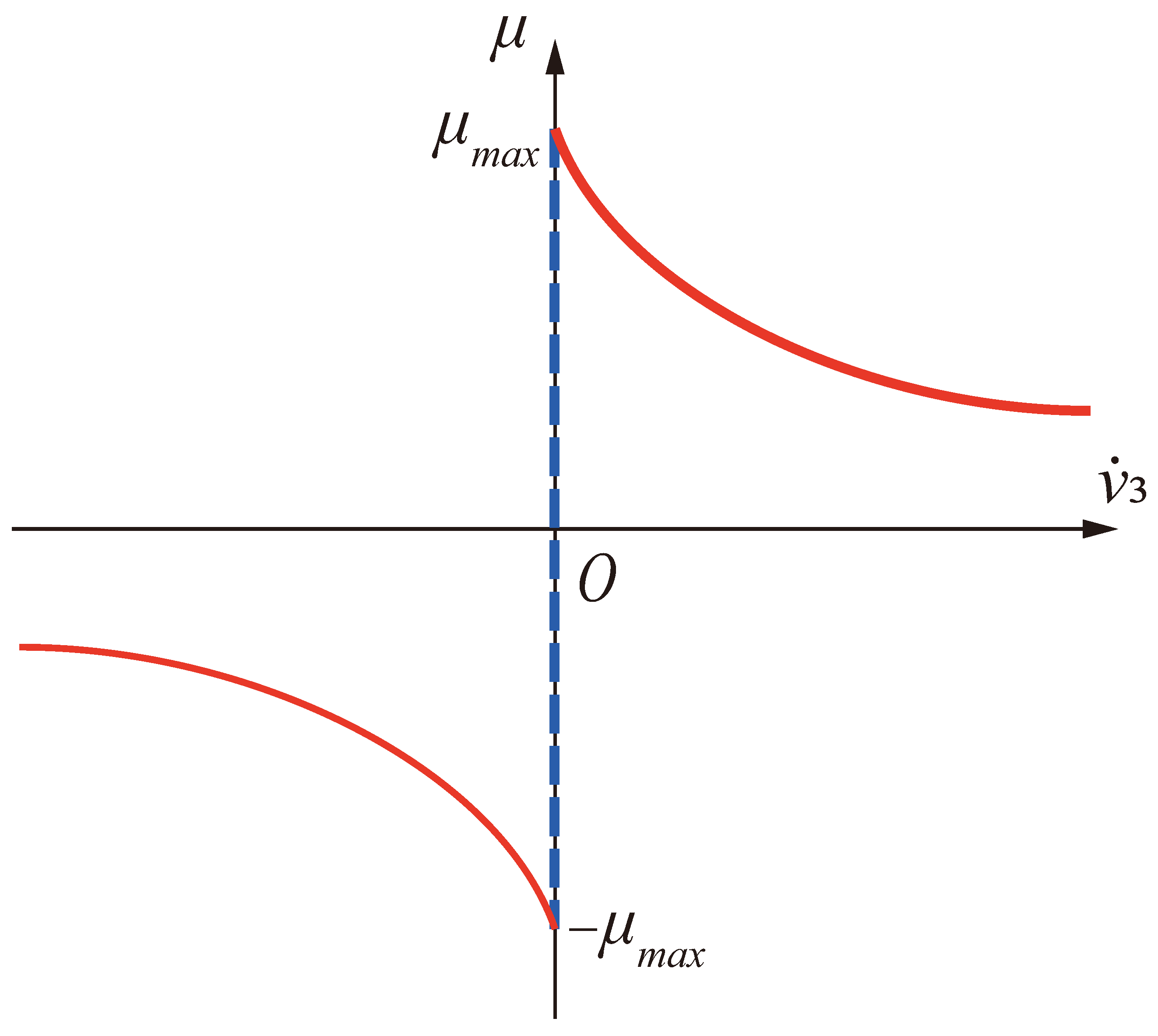
2.3. Friction Models in the Slip and Stick States

There are two states in which the motion of the wiper blade is governed by different kinds of friction. The slip state corresponds to the case where the relative velocity between the tip of the wiper blade and the windshield is nonzero. The friction acting on the tip of the wiper blade is dynamic in this case. The wiper blade is in the stick state when the relative velocity is continuously zero, in which case static friction acts on the blade.
The dynamic friction is uniquely determined by the relative velocity. As long as the stick state is maintained, the absolute value of the static friction can be taken arbitrarily in the range from zero to the maximum static friction. Hence, different models are required for the slip and stick states.
The dynamic friction in the slip state is modeled as a function of the relative velocity. The displacement along the y-axis of the tip of the wiper blade, which corresponds to v 3 in Figure 2, can be expressed as follows:
v 3 = a 1 cos ω t C l 1 cos θ l 2 cos φ tan θ 0 + l 1 sin θ + l 2 sin φ ,
where C is a constant representing the distance from the origin to the wiping surface. The relative velocity can be expressed as follows:
v 3 ˙ = a ω sin ω t + d θ d t l 1 cos θ + θ 0 cos θ 0 + d φ d t l 2 cos φ + θ 0 cos θ 0 .
In the motion of the rubber in contact with the glass, the change in the coefficient of dynamic friction under wet conditions due to the thin film of water in between the rubber blade and glass is particularly critical. A thin film of water can be formed between the wiper blade and glass because the pressure of the fluid gradually increases as the sliding velocity increases [14]. The lubrication effect of the thin film of water leads to a reduction in the coefficient of dynamic friction [13]. Thus, the relationship between the relative velocity of the tip of the second link v ˙ 3 and the coefficient of dynamic friction μ d is assumed to be as follows in the case v ˙ 3 0 :
μ d = sign v 3 ˙ A exp B | v 3 ˙ | + E ,
where the coefficient of dynamic friction is assumed to be equal to the coefficient of the maximum static friction when v 3 ˙ is zero and has a negative correlation with v 3 ˙ . The parameters A and E define the coefficient of the maximum static friction μ m a x as follows:
μ m a x = A + E .
The parameter B reflects the magnitude of the negative correlation. A, B, and E are all positive constants, and sign v 3 ˙ is the signum function, expressed as
sign v 3 ˙ = 1 , v 3 ˙ > 0 1 , v 3 ˙ < 0 .
The dynamic friction f d is then expressed as
f d = μ d N .
The normal force N is always positive, except when the jump phenomenon occurs. Therefore, the dynamic friction f d always acts in the direction opposite the relative velocity v 3 ˙ .
In the stick state, the relative velocity remains at zero continuously and the equilibrium should be maintained. The absolute value of the friction force should be less than the maximum static friction and balance the tangential force of the wiper blade. Considering the above characteristics, the static friction is defined as follows:
f s = Sign v 3 ˙ μ m a x N ,
where Sign v 3 ˙ is a set-valued function expressed as
Sign v 3 ˙ = 1 , 1 , v ˙ 3 = 0 .
By combining the two models for dynamic and static friction, the relationship between the coefficient of friction and the relative velocity is as shown in Figure 4. Given the relationship between the normal force N and the friction force f for the different states of motion, the behavior of the two links can be analyzed. For the four unknown quantities, in addition to Equations (2)–(4), the other equations in the slip and stick states are Equations (11) and (12), respectively.
By introducing the representative time T = I 2 + m 2 l g 2 2 k 2 and the representative length L = a , the dimensionless forms of Equations (2)–(4) are expressed as follows:
θ ¨ m d * l 1 * sin θ cos θ 0 + m a * l g 1 * sin ( θ + θ 0 ) + m b * l 1 * tan θ 0 cos ( θ + θ 0 ) + φ ¨ l 2 * sin φ cos θ 0 + m b * l g 2 * sin ( φ + θ 0 ) = θ ˙ 2 m d * l 1 * cos θ cos θ 0 m a * l g 1 * cos ( θ + θ 0 ) + m b * l 1 * tan θ 0 sin ( θ + θ 0 ) + φ ˙ 2 l 2 * cos φ cos θ 0 m b * l g 2 * cos ( φ + θ 0 ) + k 0 * l 1 * 1 cos θ cos θ 0 + l 2 * 1 cos φ cos θ 0 h d * + c 0 * θ ˙ l 1 * sin θ cos θ 0 + φ ˙ l 2 * sin φ cos θ 0 + N * cos θ 0 + f * sin θ 0 ω * 2 sin θ 0 cos ω * t * ,
θ ¨ m a * l 1 * l g 1 * sin θ cos θ 0 sin θ + θ 0 + m b * l 1 * 2 cos θ cos θ 0 cos θ + θ 0 + m a * l g 1 * 2 + I 1 * + φ ¨ m b * l 1 * l g 1 * cos φ θ m e * l 2 * sin φ sin θ + θ 0 cos θ 0 = θ ˙ 2 m e * l 1 * cos θ sin θ + θ 0 cos θ 0 + φ ˙ 2 m e * l 2 * cos φ sin θ + θ 0 cos θ 0 + m b * l 1 * l g 2 * sin φ θ + M k 1 * c 1 * θ ˙ + k 2 * φ θ + c 2 * φ ˙ θ ˙ + N * l 1 * sin θ + f * l 1 * cos θ m e * ω * 2 cos θ cos ω * t * ,
θ ¨ m b * l 1 * l g 2 * cos φ cos θ 0 cos θ + θ 0 + φ ¨ m b * l 2 * l g 2 * sin φ cos θ 0 sin φ + θ 0 + m b * l g 2 * 2 + I 2 * = θ ˙ 2 m b * l 1 * l g 2 * cos φ sin θ + θ 0 cos θ 0 + φ ˙ 2 m b * l 2 * l g 2 * cos φ sin φ + θ 0 cos θ 0 k 2 * φ θ c 2 * φ ˙ θ ˙ + N * l 2 * sin φ + f * l 2 * cos φ m b * l g 2 * ω * 2 cos φ cos ω * t * ,
where the dots denote derivatives with respect to the dimensionless time t * . The dimensionless parameters are as follows:
ω * = ω I 2 + m 2 l g 2 2 k 2 , l 1 * = l 1 a , l 2 * = l 2 a , l g 1 * = l g 1 a , l g 2 * = l g 2 a , h d * = h d a , m a * = m 1 m 0 + m 1 + m 2 , m b * = m 2 m 0 + m 1 + m 2 , m d * = m 0 + m 1 m 0 + m 1 + m 2 , m e * = m 1 l g 1 + m 2 l 1 m 0 + m 1 + m 2 a , I 1 * = I 1 m 0 + m 1 + m 2 a 2 , I 2 * = I 2 m 0 + m 1 + m 2 a 2 , k 0 * = k 0 I 2 + m 2 l g 2 2 k 2 m 0 + m 1 + m 2 , M k 1 * = M k 1 I 2 + m 2 l g 2 2 k 2 a 2 m 0 + m 1 + m 2 , k 2 * = k 2 I 2 + m 2 l g 2 2 k 2 a 2 m 0 + m 1 + m 2 , c 0 * = c 0 m 0 + m 1 + m 2 I 2 + m 2 l g 2 2 k 2 , c 1 * = c 1 a 2 m 0 + m 1 + m 2 I 2 + m 2 l g 2 2 k 2 , c 2 * = c 2 a 2 m 0 + m 1 + m 2 I 2 + m 2 l g 2 2 k 2 .

3. Numerical Calculation Method in Different States

3.1. Numerical Calculation Method in the Slip State

From hereon, the superscript ∗ representing dimensionless quantities is omitted for simplicity. The unknown friction force f can be eliminated by substituting Equation (11) into Equations (14)–(16). The equations for the unknown variables θ , φ , and N become
A 1 θ ¨ + B 1 φ ¨ = C 1 + N H ,
A 2 θ ¨ + B 2 φ ¨ = C 2 + N l 1 G 1 ,
A 3 θ ¨ + B 3 φ ¨ = C 3 + N l 2 G 2 ,
where A 1 , A 2 , A 3 , B 1 , B 2 , B 3 , C 1 , C 2 , C 3 , H, G 1 , and G 2 are
A 1 = m d l 1 sin θ cos θ 0 + m a l g 1 sin ( θ + θ 0 ) + m b l 1 tan θ 0 cos ( θ + θ 0 ) ,
A 2 = m a l 1 l g 1 sin θ cos θ 0 sin θ + θ 0 + m b l 1 2 cos θ cos θ 0 cos θ + θ 0 + m a l g 1 2 + I 1 ,
A 3 = m b l 1 l g 2 cos φ cos θ 0 cos θ + θ 0 ,
B 1 = l 2 sin φ cos θ 0 + m b l g 2 sin ( φ + θ 0 ) ,
B 2 = m b l 1 l g 1 cos φ θ m e l 2 sin φ sin θ + θ 0 cos θ 0 ,
B 3 = m b l 2 l g 2 sin φ cos θ 0 sin φ + θ 0 + m b l g 2 2 + I 2 ,
C 1 = θ ˙ 2 m d l 1 cos θ cos θ 0 m a l g 1 cos ( θ + θ 0 ) + m b l 1 tan θ 0 sin ( θ + θ 0 ) + φ ˙ 2 l 2 cos φ cos θ 0 m b l g 2 cos ( φ + θ 0 ) + c 0 θ ˙ l 1 sin θ cos θ 0 + φ ˙ l 2 sin φ cos θ 0 + k 0 l 1 1 cos θ cos θ 0 + l 2 1 cos φ cos θ 0 h d ω 2 sin θ 0 cos ω t ,
C 2 = θ ˙ 2 m e l 1 cos θ sin θ + θ 0 cos θ 0 + φ ˙ 2 m e l 2 cos φ sin θ + θ 0 cos θ 0 + m b l 1 l g 2 sin φ θ + M k 1 c 1 θ ˙ + k 2 φ θ + c 2 φ ˙ θ ˙ m e ω 2 cos θ cos ω t ,
C 3 = θ ˙ 2 m b l 1 l g 2 cos φ sin θ + θ 0 cos θ 0 + φ ˙ 2 m b l 2 l g 2 cos φ sin φ + θ 0 cos θ 0 k 2 φ θ c 2 φ ˙ θ ˙ m b l g 2 ω 2 cos φ cos ω t ,
H = cos θ 0 μ d sin θ 0 ,
G 1 = sin θ μ d cos θ ,
G 2 = sin φ μ d cos φ .
Using Equation (20), the normal force N is expressed in terms of θ and φ as
N = A 3 θ ¨ + B 3 φ ¨ C 3 l 2 G 2 .
Substituting Equation (33) into Equations (18) and (19) yields
A 1 A 3 H l 2 G 2 θ ¨ + B 1 B 3 H l 2 G 2 φ ¨ = C 1 C 3 H l 2 G 2 ,
A 2 l 1 A 3 G 1 l 2 G 2 θ ¨ + B 2 l 1 B 3 G 1 l 2 G 2 φ ¨ = C 2 l 1 C 3 G 1 l 2 G 2 .
Equations (34) and (35) can also be written in matrix form as follows:
a 11 a 12 a 21 a 22 θ ¨ φ ¨ = P 1 P 2 ,
where a 11 , a 12 , a 21 , a 2 , P 1 , and P 2 are
a 11 = A 1 A 3 H l 2 G 2 ,
a 12 = B 1 B 3 H l 2 G 2 ,
a 21 = A 2 l 1 A 3 G 1 l 2 G 2 ,
a 22 = B 2 l 1 B 3 G 1 l 2 G 2 ,
P 1 = C 1 C 3 H l 2 G 2 ,
P 2 = C 2 l 1 C 3 G 1 l 2 G 2 .
The differential equations for θ and φ can be rewritten as follows using Equation (36):
θ ¨ = a 22 P 1 a 12 P 2 a 11 a 22 a 12 a 21 ,
φ ¨ = a 21 P 1 + a 11 P 2 a 11 a 22 a 12 a 21 .
The state equation can then be written as Equation (45), and the Runge-Kutta method can be used for the numerical calculation of θ and φ .
d d t θ θ ˙ φ φ ˙ = θ ˙ θ ¨ φ ˙ φ ¨ .

3.2. Numerical Calculation Method in the Stick State

Unlike the slip state, a definite relationship between the friction force f and the normal force N cannot be established in the stick state. Static friction acts at the tip of the blade as a constraining force to balance the external forces acting on the wiper blade and keep the tip stationary. The holonomic constraint that the displacement of the tip cannot vary must be satisfied. A constant α is introduced to indicate the stationary position of the tip. In the stick state, the distance Φ between the tip and α should always be 0. This condition can be expressed as follows:
Φ = v 3 α = 0 ,
where the y-coordinate position of the tip v 3 is given by Equation (6). In the stick state, v 3 remains constant at α . Equation (46) is an independent equation describing the relationship between θ and φ . The dynamic behavior of the wiper blade in the stick state becomes resolvable by associating Equation (46) with Equations (14)–(16). However, because Equation (46) is not a differential equation, a set of algebraic and differential equations (ADEs) consisting of Equations (14)–(16) and (46) must be solved.
To solve this set of ADEs, Baumgarte’s stabilization method [20] is employed to modify the ADEs into a set of differential equations. The second-order differential equation:
Φ ¨ + β 1 Φ ˙ + β 2 Φ = 0
is introduced instead of Equation (46). The parameters β 1 and β 2 are both constants. The solution Φ of Equation (47) can be maintained close to 0 if β 1 and β 2 in Equation (47) have suitable values. Equation (47) can be written in dimensionless form as follows:
θ ¨ l 1 cos θ + θ 0 cos θ 0 + φ ¨ l 2 cos φ + θ 0 cos θ 0 = θ ˙ l 1 sin θ + θ 0 cos θ 0 + φ ˙ l 2 sin φ + θ 0 cos θ 0 β 1 Φ ˙ β 2 Φ ω 2 cos ω t .
Combining the differential equations and rewriting them in matrix form yields
B θ ¨ φ ¨ N f = Q ,
where the matrices B and Q are
B = b 11 b 12 b 13 b 14 b 21 b 22 b 23 b 24 b 31 b 32 b 33 b 34 b 41 b 42 0 0 ,
Q = Q 1 Q 2 Q 3 Q 4 .
The elements of B and Q are given in Appendix B.
The differential equations for θ and φ are then obtained from Equation (49) by multiplying the inverse of matrix B from the left side.

4. Behavior of Wiper Blade

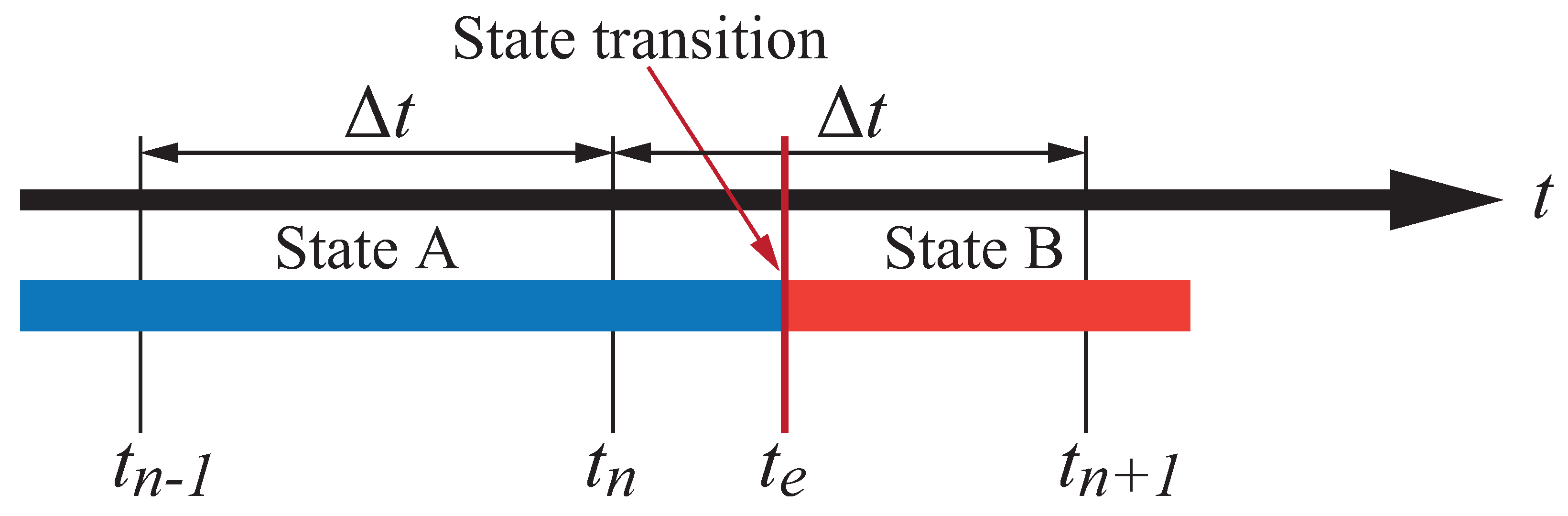
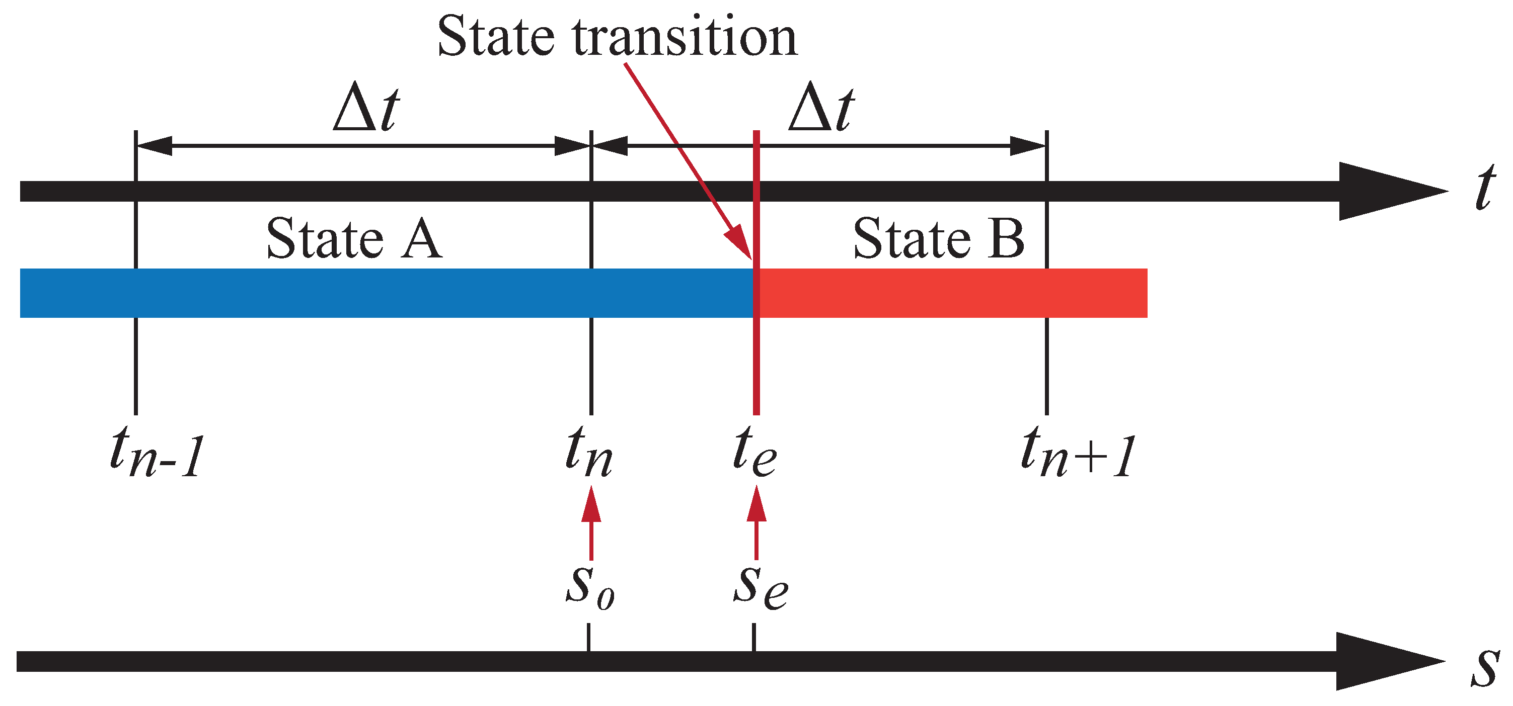
4.1. Employment of the Slack Variable Method to Obtain the Transition Time and State Variables

There are two state transitions—the transition of the friction state from slip to stick or from stick to slip and the transition of the stiffness of the first link.
Because of the nonlinearity of the governing equations, it is important to find the exact transition time and the state variables of the wiper blade at this point. In nonlinear systems, even small errors in the initial conditions may cause significant errors in the calculation results. However, as shown in Figure 5, the transient time and conditions of the wiper blade at the exact transition time t e cannot be obtained from calculations using a discrete time step size Δ t .
We introduce the slack variable method [21] to detect the transition time and calculate the conditions at that point accurately. First, the slack variable s is introduced. This variable satisfies Equation (52).
s = R t s .
Differentiating Equation (52) with respect to s gives
d s d s = 1 = d R d s = d R d t d t d s .
Deforming Equation (53) yields
d t d s = d R d t 1 .
Regarding s as an independent variable and substituting Equation (54) into the state Equation (45) yield
d d s t θ θ ˙ φ φ ˙ = d t d s d θ d t d t d s d θ ˙ d t d t d s d φ d t d t d s d φ ˙ d t d t d s = d R d t 1 θ ˙ d R d t 1 θ ¨ d R d t 1 φ ˙ d R d t 1 φ ¨ d R d t 1 .
In the calculations of using the discrete time, we consider the case in which the state transition occurs in the interval [ t n , t n + 1 ] , as shown in Figure 6. The calculation then starts again from t n using s as the independent variable and t as the dependent variable. The exact transition time t e and the conditions of the wiper blade at this time can be obtained by integrating Equation (55) from s 0 to s e , where s e is defined later.

4.2. Conditions of State Transitions

4.2.1. Transition from Slip to Stick State

When applying the slack variable method, it is essential to apply the appropriate R function for different state transitions.
In the slip state, the relative velocity v ˙ 3 is assumed to be nonzero. The state transition from slip to stick occurs when v ˙ 3 becomes zero. Hence, the R function for the state transition from slip to stick is as follows:
R = v ˙ 3 = ω sin ω t + l 1 θ ˙ cos θ + θ 0 cos θ 0 + l 2 φ ˙ cos φ + θ 0 cos θ 0 .
The derivative of t with respect to s is
d t d s = d R d t 1 = v ¨ 3 1 = ω 2 cos ω t + l 1 θ ¨ cos θ + θ 0 cos θ 0 + l 2 φ ¨ cos φ + θ 0 cos θ 0 l 1 θ ˙ 2 sin θ + θ 0 cos θ 0 l 2 φ ˙ 2 sin φ + θ 0 cos θ 0 1 .
The exact transition time is obtained by substituting Equation (57) into Equation (55) and integrating the result with respect to s from s 0 to s e .

4.2.2. Transition from Stick to Slip State

In the calculations for the stick state, if the absolute value of the static friction force f is greater than the maximum friction force μ m a x N , the force equilibrium of the wiper blade will be destroyed. Hence, when the static friction force f reaches the maximum friction force μ m a x N , the state transitions from stick to slip. The R function for the state transition from stick to slip is as follows:
R = | f | μ m a x N .
The derivative of t with respect to s is
d t d s = d R d t 1 = d | f | d t μ m a x d N d t 1 ,
which can also be obtained by differentiating Equation (49). The exact transition time is obtained by substituting Equation (59) into Equation (55) and integrating from s 0 to s e , as described above. Here, s 0 is the value of | f | μ m a x N at t n and s e is the value of | f | μ m a x N at t e , which is zero.

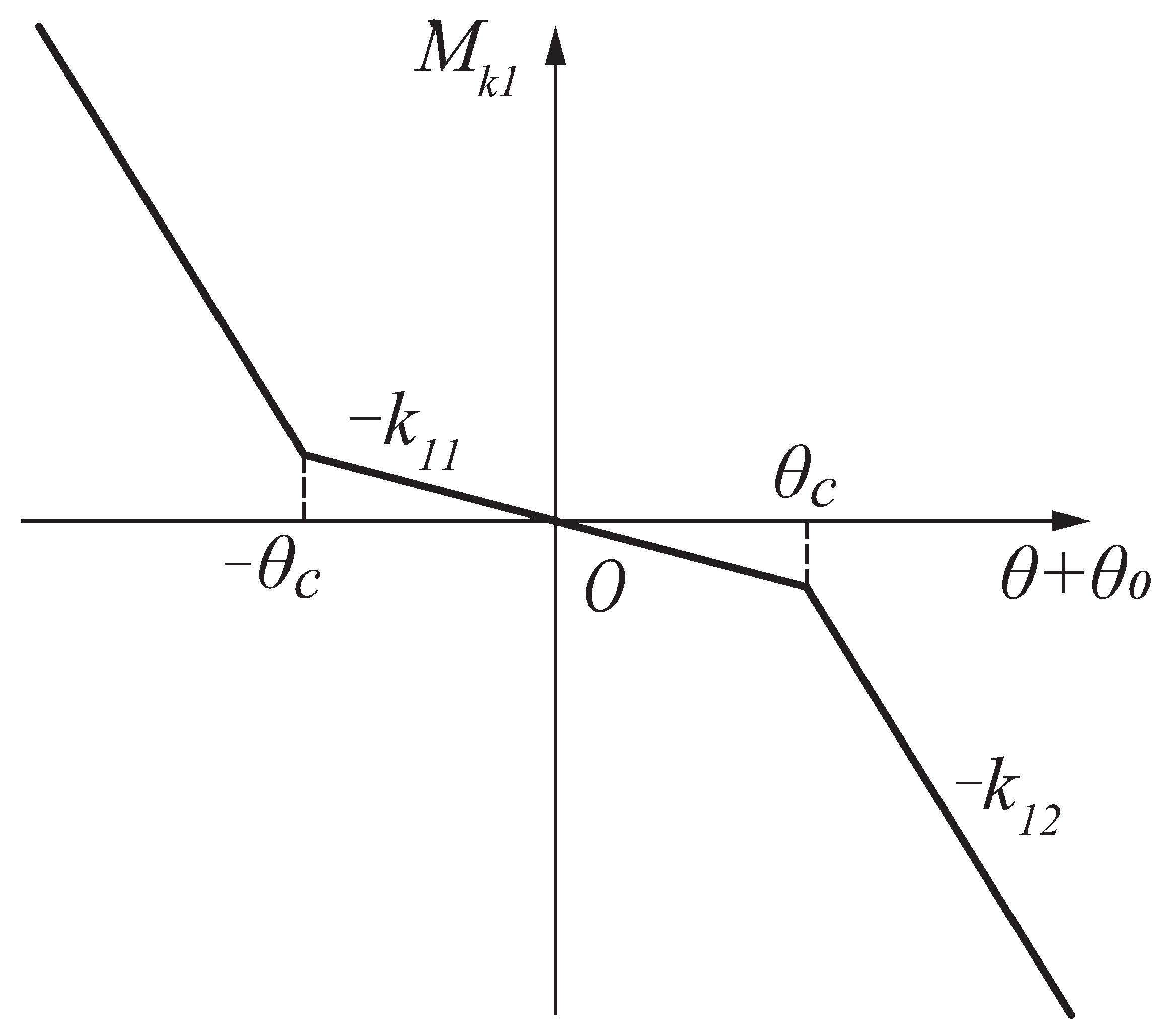
4.2.3. Transition of the Rotational Stiffness

In addition to the above two transitions, there is also a state transition in the rotational stiffness, because the first link is piecewise linearly related to the shoulder contact, as shown in Figure 3. The state transition occurs when the angle of the first link θ passes through θ c while in motion. The R function for this transition can be set as follows:
R = θ .
The derivative of t with respect to s can be easily computed as
d t d s = d R d t 1 = θ ˙ 1 .
The exact transition time is determined through the same process as for the stick–slip transitions, except that the start and end points of the integration are different. The calculation starts at s 0 , which is the angle θ at t n , and ends at s e , which is the angle at which shoulder contact occurs, θ c .

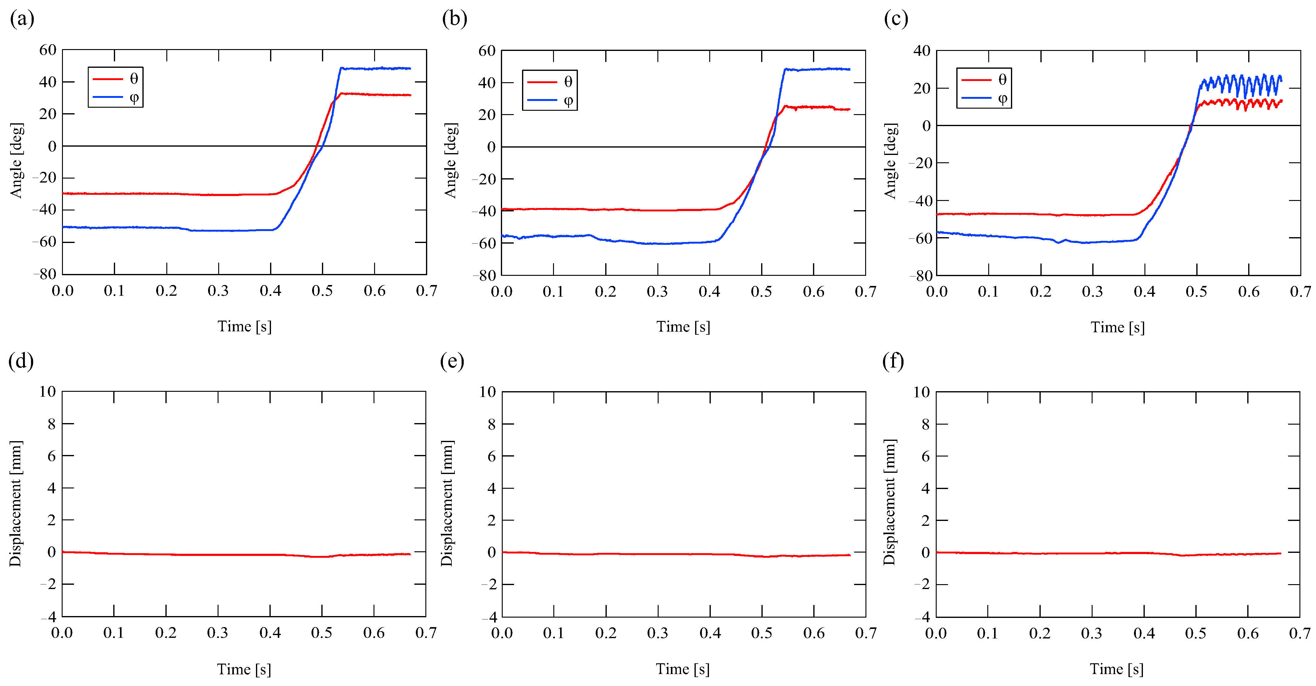
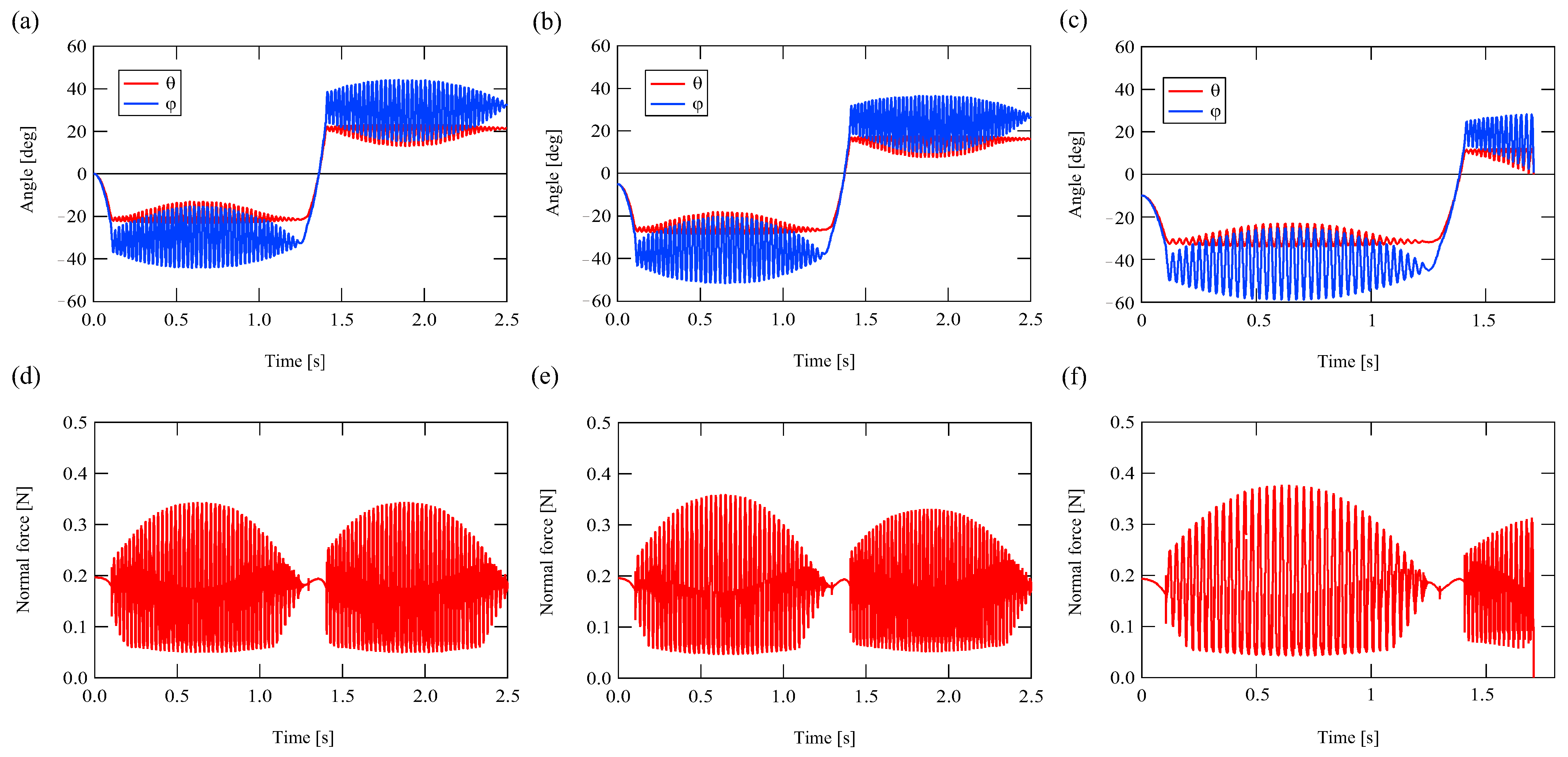
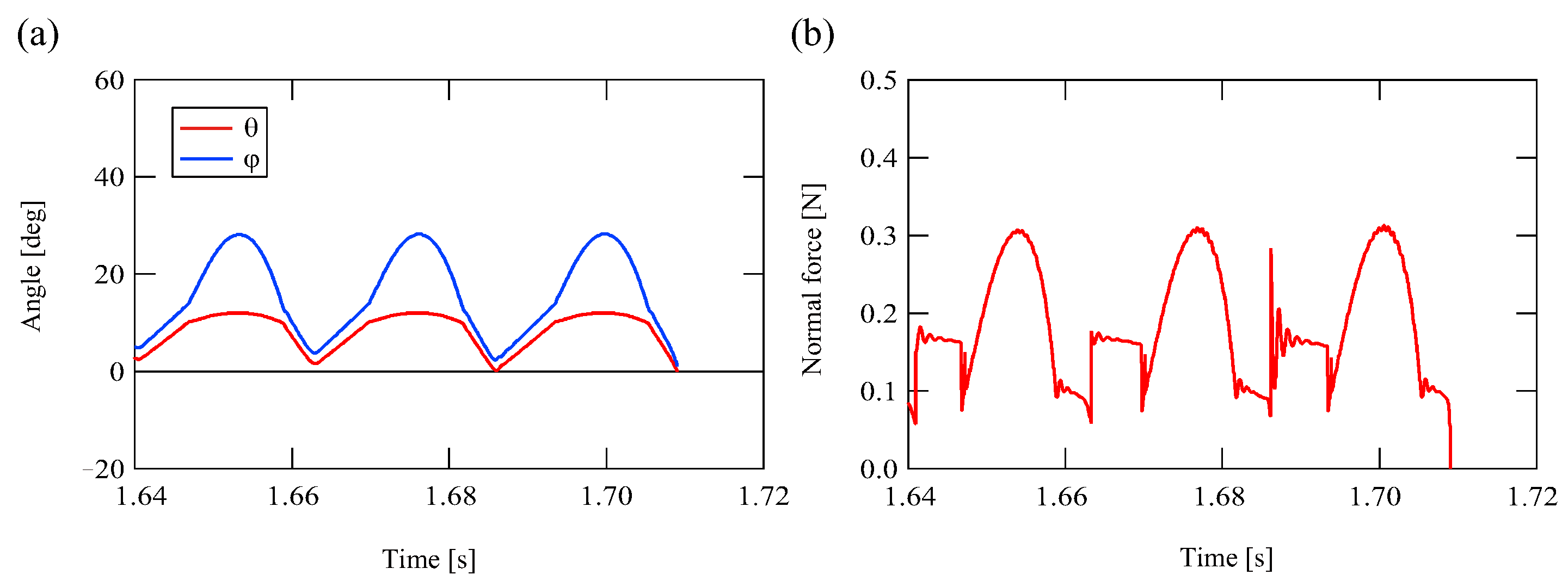
4.3. Numerical Calculation Results

Following the method described above, a numerical calculation program was developed in Matlab®, and the differential equation solver ODE45 was used to obtain solutions. The parameter values in the program were obtained from the actual wiper blade used in subsequent experiments. The maximum speed of the head, which is determined by a and ω , was found to be about 125 mm/s. The dynamic friction in the velocity region from 0–125 mm/s exhibits strongly nonlinear characteristics. The initial condition for the numerical calculation was the stick state. The calculations terminated at the end of one round trip of the wiper blade. The parameters used in the program are listed in Table 1.
The numerical results in Figure 7 show the relationship between the attack angle and the jump phenomenon. Figure 8 shows enlarged views of Figure 7c,f around the jump phenomenon. Figure 7a,b show the changes in the angles θ and φ , while Figure 7d,e show the change in the normal force N of the wiper blade over one reciprocal motion with attack angles of 0 and 5 degrees, respectively. From the figures, it can be seen that the wiper blade does not jump under these conditions. Figure 7c shows the changes in θ and φ with an attack angle of 10 degrees. In this condition, the normal force N changes direction, i.e., the jump phenomenon occurs, as shown in Figure 7f and Figure 8b. Figure 7c and Figure 8a confirm that the two angles become 0 at the same time when the jump phenomenon occurs, which does not happen in other conditions. Around the reversal point, both angles become 0 at the same time, as shown in Figure 7d–f. However, the normal force N does not become 0, and so, the jump phenomenon does not occur. Therefore, the occurrence of the stick–slip motion is a necessary condition for producing the jump phenomenon.

5. Experimental Results

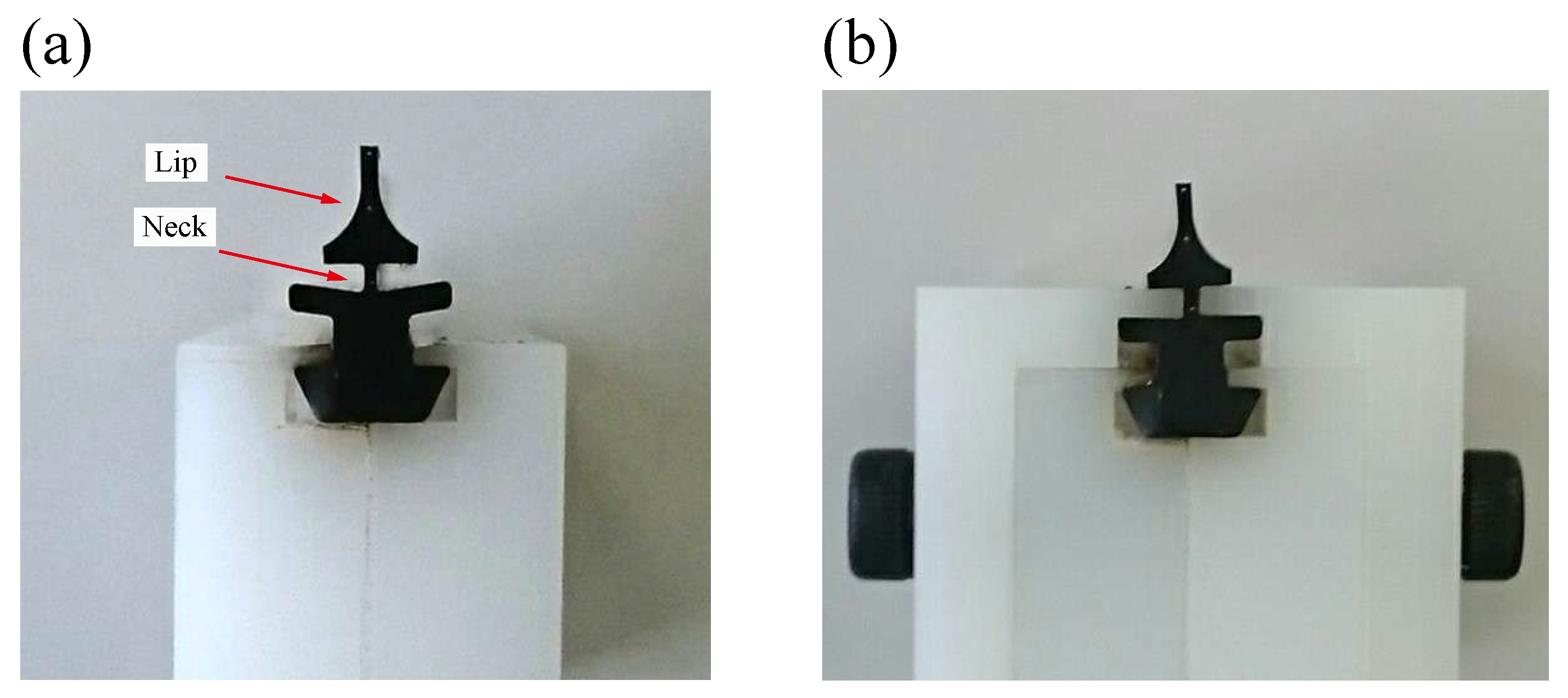
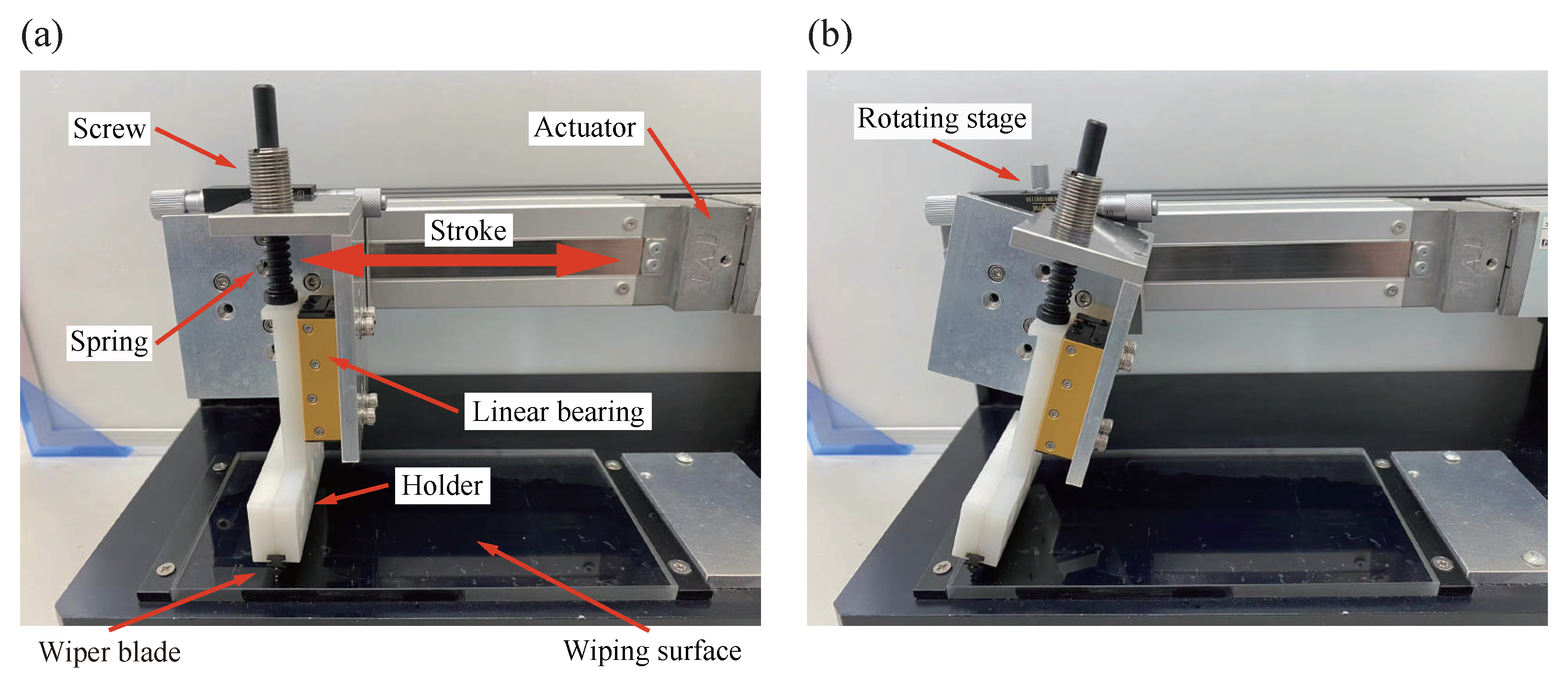
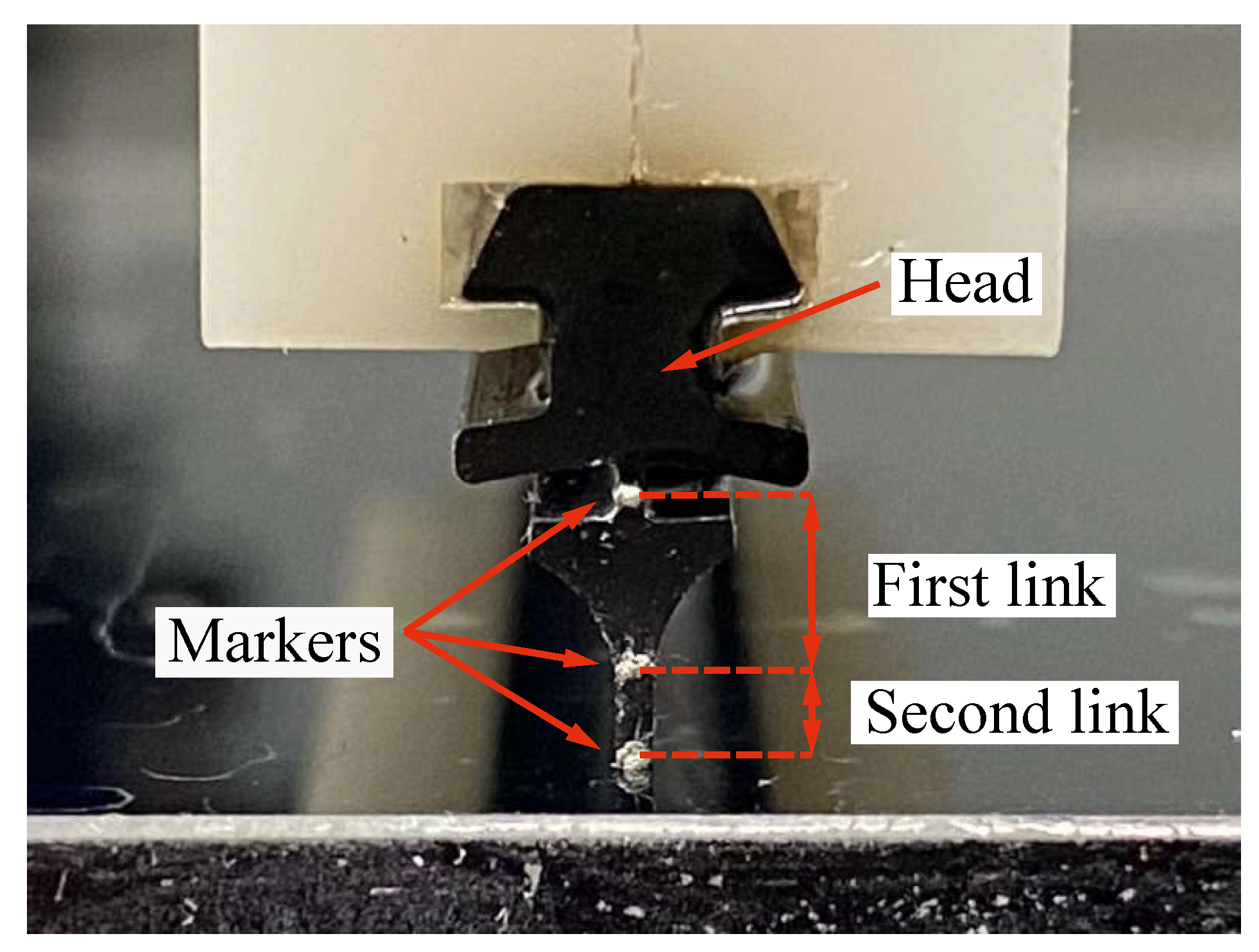
5.1. Experimental Apparatus and Procedure

To verify the accuracy of the theoretical analysis, the experimental setup shown in Figure 9 was created. There is a spring with a spring constant of 1.43 N/mm and an original length of 0.2 m above the holder. A pressure force is supplied to the holder by rotating the screw to change the length of the spring. This is equivalent to determining the value of h d . The entire system can move liberally within the stroke of the linear bearing. The wiper blade is clamped by the holder and driven by the actuator to perform a reciprocating motion on the wiping surface. Before each experiment, water was sprayed on the wiping surface.
An enlarged view of the wiper blade is shown in Figure 10. There are three white dots marked on the neck, the center of rotation of the second link, and the tip of the wiper blade.
The motion of the wiper blade was filmed by a high-speed video camera (FASTCAM-APX RS 250 K, Photron Inc., San Diego, CA, USA) with a frame rate of 3000 fps at a 1024 × 512 pixel resolution on a screen measuring 3.165 × 10 2 m × 1.583 × 10 2 m. Thus, each pixel had dimensions of 3.091 × 10 5 m. We conducted two experiments for attack angles of 0, 10, and 18 degrees. In the first experiment, the camera recorded the location at which the jump phenomenon occurs during the wiping process. In the second experiment, the filming position was located around the reversal point of the wiper blade.

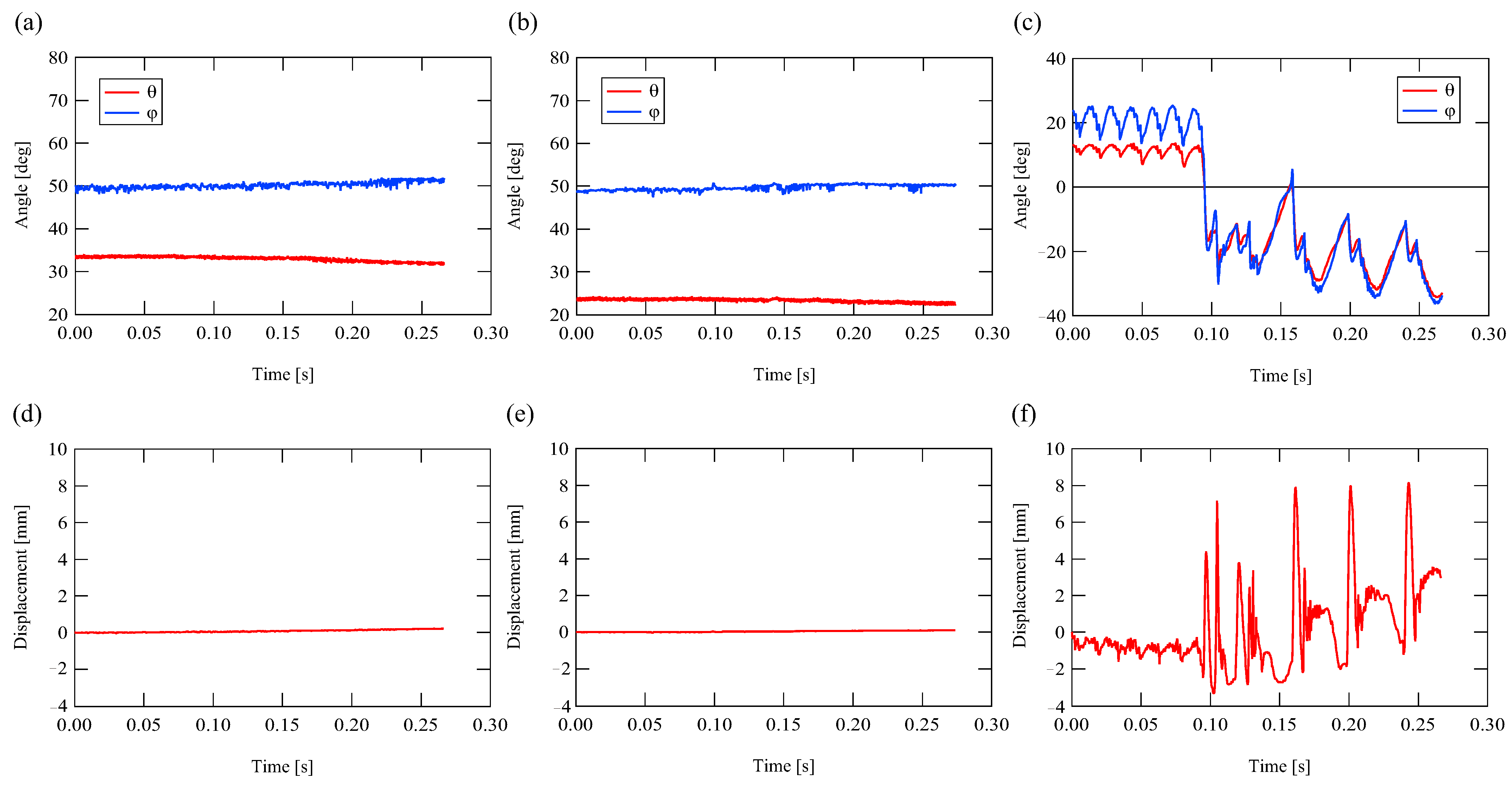
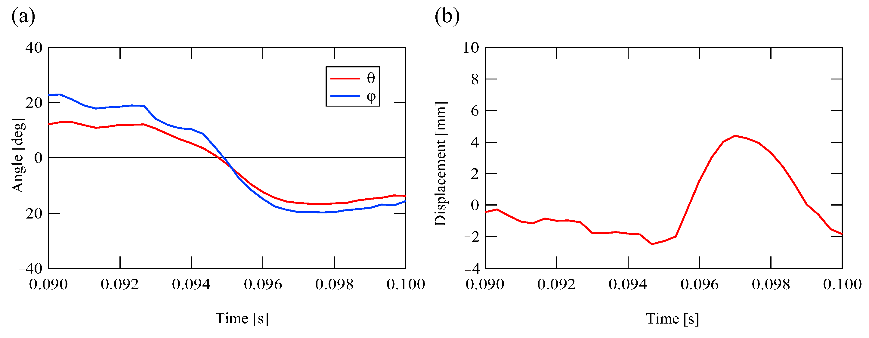
5.2. Experimental Results

After filming, we used image analysis software (Dipp-Motion V, DITECT Corp., Toronto, ON, Canada) to track the markers on the wiper blade in advance. From the tracking results, we obtained the angular changes of the two links and the change in displacement of the tip of the wiper blade in the direction perpendicular to the wiping surface.
Figure 11 shows the experimental results obtained during the wiping process; Figure 12 shows an enlarged view of Figure 11c,f near the occurrence of the jump phenomenon. Figure 11d,e confirm that attack angles of 0 and 10 degrees do not produce the jump phenomenon. When the attack angle is 18 degrees, however, the jump phenomenon occurs, as shown in Figure 11f and Figure 12b. We can also confirm from Figure 11c and Figure 12a that the angles θ and φ converge to 0 at the same time when the jump phenomenon occurs. In turn, these two angles do not converge to 0 at the same time when no jump phenomenon occurs, as shown in Figure 11a,b.
The experiments also suggested that the stick–slip motion does not occur around the reversal point. Thus, even if the angles become 0 at the same time, there is no jump phenomenon. Figure 13 shows the experimental results obtained around the reversal point with different attack angles. Figure 13d–f confirm that the wiper blade does not jump away from the wiping surface around the reversal point at the different attack angles. This is despite the two angles becoming 0 at the same time in this process, as shown in Figure 13a–c.
There are quantitative discrepancies between the theoretical and experimental results. For example, in the theoretical results, the angles of the two links vary periodically also in the state where the jump phenomenon does not occur, as in Figure 7a,b. However, the angles of the two links do not change significantly in the experiments in such a state, as in Figure 11a,b. Besides, although it was theoretically and experimentally shown that the jump phenomenon becomes more likely as the attack angle increases, the theoretical and experimental values of the attack angle where the jump phenomenon starts to occur are different quantitatively. In the theoretical result, a 10-degree attack angle produces the jump-up phenomenon, as shown in Figure 7c,f. However, there is no jump phenomenon with a 10-degree attack angle in the experimental result, as shown in Figure 11b,e. In addition, in the theoretical results where the jump phenomenon occurs, the angles of the two links are very close to 0 at about 1.66 s and 1.68 s before they become 0 at the same time, as in Figure 8a. However, the angles of the two links are not so close to 0 at about 0.05 s, 0.06 s and 0.07 s before they become 0 at the same time in the experimental results shown in Figure 11c. The actual wiper blade is an infinite-degree-of-freedom elastomer rather than the low-degree-of-freedom two-link model used in the theoretical analysis. This is the reason for the quantitative discrepancies between the theoretical and experimental results.

6. Conclusions

In this study, we analyzed the occurrence of the jump phenomenon of a wiper blade depending on the attack angle. We introduced a two-degree-of-freedom model of a wiper blade and considered effects such as dynamic and static friction, nonlinear rotation stiffness, and attack angle on the dynamic behavior of the wiper blade. In the slip state, we considered the negative slope between the dynamic friction and the relative velocity. In the stick state, we used Baumgarte’s stabilization method for the numerical calculations. As the numerical simulation results of nonlinear systems are highly dependent on the initial conditions, we also used the slack variable method to determine the exact time of each state transition and the state of motion at that point. When considering the attack angle, the normal force N is no longer independent, but is influenced by the friction force f. We established a simulation program based on these considerations. The simulation results indicated that a larger attack angle made the jump phenomenon more likely. The reason for the jump phenomenon can be attributed to the angle of the two links becoming 0 at the same time during the stick–slip motion of the wiper blade. In contrast, if the wiper blade is not in stick–slip motion, such as during the process of reversal, the jumping phenomenon does not occur even if the two angles become 0 at the same time. The results of our theoretical analysis were confirmed by experiments conducted using an actual wiper blade. The theoretical analysis for the model of wiper blade considering a constant attack angle can be proven to be effective. The attack angle varies continuously on the practical windshield of the car. The present theoretical approach can be easily applicable to such a practical situation.

Author Contributions

Conceptualization, methodology, project administration, supervision, and writing—review and editing, H.Y.; conceptualization, investigation, software, visualization, and writing—original draft, Z.Z.; Funding acquisition, resources, K.K. All authors have read and agreed to the published version of the manuscript.

Funding

This work was supported by MITSUBA Co., Ltd.

Institutional Review Board Statement

Not applicable.

Informed Consent Statement

Not applicable.

Data Availability Statement

Data sharing does not apply to this article as no datasets were generated or analyzed during the current study.

Acknowledgments

We thank Stuart Jenkinson for editing a draft of this manuscript.

Conflicts of Interest

The authors declare no potential conflict of interest with respect to the research, authorship, and/or publication of this article.

Nomenclature

m 0 weight of the head
m 1 weight of the first link
m 2 weight of the second link
I 1 moment of inertia of the first link about the center of gravity
I 1 moment of inertia of the second link about the center of gravity
l 0 original length of the head spring
l 1 length of the first link
l 2 length of the second link
l g 1 distance from the top to the center of gravity of the first link
l g 2 distance from the top to the center of gravity of the second link
k 0 spring constant of the head
k 11 rotation stiffness of the first link without shoulder contact
k 12 rotation stiffness of the first link with shoulder contact
k 2 rotation stiffness of the second link
c 0 damping of the head
c 1 damping of the first link
c 2 damping of the second link
aamplitude of the oscillator
ω frequency of the oscillator
h d initial compression of the head spring
θ angle of the first link
φ angle of the second link
v 3 displacement along the y-axis of the tip of the wiper blade
θ c angle of shoulder contact
μ d coefficient of dynamic friction
μ m a x maximum static friction
α y-direction coordinate of the tip after transition from the slip state to the stick state
Nnormal force acting on the tip
ffriction force acting on the tip

Appendix A. Process of Deriving the Equations of Motion

The model of the wiper blade can be divided into a free body diagram, as shown in Figure A1.
Figure A1. Free body diagram of the model.
Applsci 12 04112 g0a1
The equations of motion for each part are as follows:
m 0 u ¨ = F u 1 F s + F d cos θ 0 + F 0 sin θ 0 ,
m 0 v ¨ = F v 1 + F s + F d sin θ 0 + F 0 cos θ 0 ,
m 1 u ¨ 1 = F u 1 + F u 2 ,
m 1 v ¨ 1 = F v 1 + F v 2 ,
m 2 u ¨ 2 = F u 2 N ,
m 2 v ¨ 2 = F v 2 + f .
Combining Equations (A1) and (A2) and eliminating the internal forces through Equations (A3)–(A6), we obtain
m 0 u ¨ + m 1 u 1 ¨ + m 2 u 2 ¨ cos θ 0 + m 0 v ¨ + m 1 v 1 ¨ + m 2 v 2 ¨ sin θ 0 + N cos θ 0 + f sin θ 0 = F s + F d .
The equations of rotation of the two links are as follows:
I 1 θ ¨ = F u 1 l g 1 sin θ + F v 1 l g 1 cos θ F u 2 l 1 l g 1 sin θ + F v 2 l 1 l g 1 cos θ + M k 1 c 1 θ ˙ + k 2 φ θ + θ 0 + c 2 φ ˙ θ ˙ ,
I 2 φ ¨ = F u 2 l g 2 sin φ + F v 2 l g 2 cos φ + N l 2 l g 2 sin φ + f l 2 l g 2 cos φ k 2 φ θ + θ 0 c 2 φ ˙ θ ˙ .
The distance from the origin to the wiping surface is fixed at a certain constant value. This distance, named C, is defined as
C = l 0 + l 1 + l 2 h d cos θ 0 .
The variation of the length of the spring k 0 can also be expressed as
Δ l = l 1 1 cos θ cos θ 0 + l 2 1 cos φ cos θ 0 h d .
Thus, the restoring force F s and damping force F d can be expressed as
F s = k 0 Δ l = k 0 l 1 1 cos θ cos θ 0 + l 2 1 cos φ cos θ 0 h d ,
F d = c 0 Δ l ˙ = c 0 θ ˙ l 1 sin θ cos θ 0 + φ ˙ l 2 sin φ cos θ 0 .
The wiper is driven by the reciprocating motion of the head. The reciprocating motion is given as a simple harmonic oscillation of frequency ω and amplitude a, i.e.,
y = a 1 cos ω t .
The geometric relationships of each coordinate are as follows:
u = C l 1 cos θ l 2 cos φ ,
v = y C l 1 cos θ l 2 cos φ tan θ 0 ,
u 1 = C l 1 cos θ l 2 cos φ + l g 1 cos θ ,
v 1 = y C l 1 cos θ l 2 cos φ tan θ 0 + l g 1 sin θ ,
u 2 = C l 2 cos φ + l g 2 cos φ ,
v 2 = y C l 1 cos θ l 2 cos φ tan θ 0 + l 1 sin θ + l g 2 sin φ .
Substituting Equations (A12), (A13), and (A15)–(A20) into Equations (A7)–(A9), we obtain Equations (2)–(4).

Appendix B. Elements of Matrices B and Q

b 11 = m d l 1 sin θ cos θ 0 + m a l g 1 sin ( θ + θ 0 ) + m b l 1 tan θ 0 cos ( θ + θ 0 ) ,
b 12 = l 2 sin φ cos θ 0 + m b l g 2 sin ( φ + θ 0 ) ,
b 13 = cos θ 0 ,
b 14 = sin θ 0 ,
b 21 = m a l 1 l g 1 sin θ cos θ 0 sin θ + θ 0 + m b l 1 2 cos θ cos θ 0 cos θ + θ 0 + m a l g 1 * 2 + I 1 ,
b 22 = m b l 1 l g 1 cos φ θ m e l 2 sin φ sin θ + θ 0 cos θ 0 ,
b 23 = l 1 sin θ ,
b 24 = l 1 cos θ ,
b 31 = m b l 1 l g 2 cos φ cos θ 0 cos θ + θ 0 ,
b 32 = m b l 2 l g 2 sin φ cos θ 0 sin φ + θ 0 + m b l g 2 2 + I 2 ,
b 33 = l 2 sin φ ,
b 34 = l 2 cos φ ,
b 41 = l 1 cos θ + θ 0 cos θ 0 ,
b 42 = l 2 cos φ + θ 0 cos θ 0 ,
Q 1 = θ ˙ 2 m d l 1 cos θ cos θ 0 m a l g 1 cos ( θ + θ 0 ) + m b l 1 tan θ 0 sin ( θ + θ 0 ) + φ ˙ 2 l 2 cos φ cos θ 0 m b l g 2 cos ( φ + θ 0 ) + k 0 l 1 1 cos θ cos θ 0 + l 2 1 cos φ cos θ 0 h d + c 0 θ ˙ l 1 sin θ cos θ 0 + φ ˙ l 2 sin φ cos θ 0 ω 2 sin θ 0 cos ω t ,
Q 2 = θ ˙ 2 m e l 1 cos θ sin θ + θ 0 cos θ 0 + φ ˙ 2 m e l 2 cos φ sin θ + θ 0 cos θ 0 + m b l 1 l g 2 sin φ θ + M k 1 c 1 θ ˙ + k 2 φ θ + c 2 φ ˙ θ ˙ m e ω 2 cos θ cos ω t ,
Q 3 = θ ˙ 2 m b l 1 l g 2 cos φ sin θ + θ 0 cos θ 0 + φ ˙ 2 m b l 2 l g 2 cos φ sin φ + θ 0 cos θ 0 k 2 φ θ c 2 φ ˙ θ ˙ m b l g 2 ω 2 cos φ cos ω t ,
Q 4 = θ ˙ l 1 sin θ + θ 0 cos θ 0 + φ ˙ l 2 sin φ + θ 0 cos θ 0 β 1 Φ ˙ β 2 Φ ω 2 cos ω t .

Appendix C. Experimental Identification of the Parameters Expressing the Stiffness and Damping in the Analytical Model

The parameters related to the rotational stiffness and damping of the two links at the two joints in the analytical model were experimentally identified by using the free oscillations of the actual wiper blade.
First, we set the wiper blade upside down, as shown in Figure A2. We experimentally obtained the free oscillations in the cases when the neck part is free and fixed. These two cases correspond to the states where only the first link and only the second one can be rotated, respectively.
Figure A2. Two fixation methods of the experimental setup. (a) The neck can be rotated. (b) The neck is fixed.
Applsci 12 04112 g0a2
The free vibrations were recorded using a high-speed video camera. Then, the markers made on the wiper blade in advance were traced. From the tracking data, the angle variation of the free vibrations in both cases can be obtained. In turn, the natural frequency and damping ratio of the free vibrations can be derived. The inverted wiper blade can be regarded as the link vibrating about a point as shown in Figure A3.
Figure A3. Model of inverted wiper blade. (a) Static inverted state. (b) Rotating state.
Applsci 12 04112 g0a3
The mass of the link is m. The moment of inertia of this rigid body around the origin is I. The distance from the center of gravity of this rigid body to the origin is l g . The rotation stiffness and damping of this link is k and c, respectively. The equation of motion for this system is
I θ ¨ + c θ ˙ + k θ m g l g sin θ = 0 .
This equation can be rewritten as
θ ¨ + 2 ζ ω n θ ˙ + ω n 2 θ = 0 ,
where ζ and ω n are, respectively,
ζ = c 2 I k m g l g ,
ω n = k m g l g I .
When ζ < 1 , the solution of Equation (A40) is
θ = A e ζ ω n t cos ( ω d t + φ ) ,
where ω d = ω n 1 ζ 2 . A and φ in Equation (A43) are determined by the initial condition. The solution corresponds to the time history of the experimentally obtained free oscillation. Since the experimentally obtained damping ratio is about 0.1, the frequency of damped free vibration ω d is almost the same as the natural frequency ω n . Regarding the experimentally obtained frequency as f n , the following equation can be obtained:
ω n = 2 π f n = k m g l g I .
The rotation stiffness k can be derived from Equation (A44).
k = ( 2 π f n ) 2 I + m g l g .
Substituting Equation (A44) into Equation (A41) yields
ζ = c 2 I k m g l g = c 4 π f n I .
In turn, the damping c can be derived as
c = 4 π f n I ζ .

References

  1. Grenouillat, R.; Leblanc, C. Simulation of chatter vibrations for wiper systems. SAE Tech. Paper. 2002. [Google Scholar] [CrossRef]
  2. Awang, I.M.; Abd Ghani, B.; Abd Rahman, R.; Zain, M.Z.M. Complex eigenvalue analysis of windscreen wiper chatter noise and its suppression by structural modifications. Int. J. Veh. Struct. Syst. 2009, 1, 24–29. [Google Scholar] [CrossRef]
  3. Lancioni, G.; Lenci, S.; Galvanetto, U. Dynamics of windscreen wiper blades: Squeal noise, reversal noise and chattering. Int. J. Non-Linear Mech. 2016, 80, 132–143. [Google Scholar] [CrossRef]
  4. Okura, S.; Sekiguchi, T.; Oya, T. Dynamic analysis of blade reversal behavior in a windshield wiper system. SAE Trans. 2000, 109, 183–192. [Google Scholar]
  5. Zolfagharian, A.; Zain, M.M.; AbuBakar, A.R.; Hussein, M. Particle swarm optimization approach on flexible structure at wiper blade system. Proc. World Acad. Sci. Eng. Technol. 2011, 18, 97–102. [Google Scholar]
  6. Koenen, A.; Sanon, A. Tribological and vibroacoustic behavior of a contact between rubber and glass (application to wiper blade). Tribol. Int. 2007, 40, 1484–1491. [Google Scholar] [CrossRef]
  7. Leine, R.I.; Nijmeijer, H. Dynamics and Bifurcations of Non-Smooth Mechanical Systems; Springer Science & Business Media: Berlin/Heidelberg, Germany, 2013; Volume 18, pp. 39–46. [Google Scholar]
  8. Nakano, K. Two dimensionless parameters controlling the occurrence of stick-slip motion in a 1-DOF system with Coulomb friction. Tribol. Lett. 2006, 24, 91–98. [Google Scholar] [CrossRef]
  9. Bódai, G.; Goda, T.J. Friction force measurement at windscreen wiper/glass contact. Tribol. Lett. 2012, 45, 515–523. [Google Scholar] [CrossRef]
  10. Le Rouzic, J.; Le Bot, A.; Perret-Liaudet, J.; Guibert, M.; Rusanov, A.; Douminge, L.; Bretagnol, F.; Mazuyer, D. Friction-induced vibration by Stribeck’s law: Application to wiper blade squeal noise. Tribol. Lett. 2013, 49, 563–572. [Google Scholar] [CrossRef]
  11. Reddyhoff, T.; Dobre, O.; Le Rouzic, J.; Gotzen, N.A.; Parton, H.; Dini, D. Friction induced vibration in windscreen wiper contacts. J. Vib. Acoust. 2015, 137, 041009. [Google Scholar] [CrossRef]
  12. Unno, M.; Shibata, A.; Yabuno, H.; Yanagisawa, D.; Nakano, T. Analysis of the behavior of a wiper blade around the reversal in consideration of dynamic and static friction. J. Sound Vib. 2017, 393, 76–91. [Google Scholar] [CrossRef]
  13. Deleau, F.; Mazuyer, D.; Koenen, A. Sliding friction at elastomer/glass contact: Influence of the wetting conditions and instability analysis. Tribol. Int. 2009, 42, 149–159. [Google Scholar] [CrossRef]
  14. Bódai, G.; Goda, T.J. Sliding friction of wiper blade: Measurement, FE modeling and mixed friction simulation. Tribol. Int. 2014, 70, 63–74. [Google Scholar] [CrossRef]
  15. Chevennement-Roux, C.; Dreher, T.; Alliot, P.; Aubry, E.; Lainé, J.P.; Jézéquel, L. Flexible wiper system dynamic instabilities: Modelling and experimental validation. Exp. Mech. 2007, 47, 201–210. [Google Scholar] [CrossRef]
  16. Min, D.; Jeong, S.; Yoo, H.H.; Kang, H.; Park, J. Experimental investigation of vehicle wiper blade’s squeal noise generation due to windscreen waviness. Tribol. Int. 2014, 80, 191–197. [Google Scholar] [CrossRef]
  17. Mohamad, S.M.; Othman, N.; Sharif, I.; Zain, M.M.; Bakar, A.A. Dynamic behaviour and characteristics of rubber blade car performance. Int. J. Automot. Mech. Eng. 2019, 16, 6437–6452. [Google Scholar] [CrossRef]
  18. Lee, C.E.; Kim, H.K. Analysis of the Cross-Sectional Shape and Wiping Angle of a Wiper Blade. SAE Int. J. Mater. Manuf. 2020, 13, 183–194. [Google Scholar] [CrossRef]
  19. Chen, T.J.; Hong, Y.J. Geometric Analysis of the Vibration of Rubber Wiper Blade. Taiwan. J. Math. 2021, 25, 491–516. [Google Scholar] [CrossRef]
  20. Baumgarte, J. Stabilization of constraints and integrals of motion in dynamical systems. Comput. Methods Appl. Mech. Eng. 1972, 1, 1–16. [Google Scholar] [CrossRef]
  21. Turner, J.D. On the simulation of discontinuous functions. J. Appl. Mech. 2001, 68, 751–757. [Google Scholar] [CrossRef]
Figure 1. Cross-section of wiper system with attack angle. (a) Shoulder stays away from the head; (b) shoulder contacts the head.
Applsci 12 04112 g001
Figure 2. Two-link model of wiper system. (a) Upright state; (b) buckled state.
Applsci 12 04112 g002
Figure 3. Restoring moment of the first link. k 11 and k 12 are the rotation stiffness of the shoulder with or without head contact, respectively. θ c is the angle at which the shoulder begins to contact the head.
Applsci 12 04112 g003
Figure 4. Relationship between coefficient of friction and relative velocity of wiper blade and wiping surface.
Applsci 12 04112 g004
Figure 5. Exact state transition time and discrete calculation time. t e : exact transition time; t n 1 , t n , t n + 1 : discrete calculation times.
Applsci 12 04112 g005
Figure 6. Process of slack variable method.
Applsci 12 04112 g006
Figure 7. Behavior of wiper blade zero and nonzero attack angle. (a) Angular displacements of two links with zero attack angle. (b) Angular displacements of two links with 5-degree attack angle. (c) Angular displacements of two links with 10-degree attack angle. (d) Normal force of wiper blade with zero attack angle. (e) Normal force of wiper blade with 5-degree attack angle. (f) Normal force of wiper blade with 10-degree attack angle.
Applsci 12 04112 g007
Figure 8. Enlarged view of Figure 7c,f from 1.64–1.72 s. Panels (a) and (b) correspond to Figure 7c,f, respectively.
Applsci 12 04112 g008
Figure 9. Experimental apparatus (a) without attack angle and (b) with an 18-degree attack angle.
Applsci 12 04112 g009
Figure 10. Enlarged view of the wiper blade.
Applsci 12 04112 g010
Figure 11. Experimental results during wiping process with zero and nonzero attack angles. (a) Angular displacements of two links with zero attack angle. (b) Angular displacements of two links with 10-degree attack angle. (c) Angular displacements of two links with 18-degree attack angle. (d) Variation of y-coordinate of the tip with zero attack angle. (e) Variation of y-coordinate of the tip with 10-degree attack angle. (f) Variation of y-coordinate of the tip with 18-degree attack angle.
Applsci 12 04112 g011
Figure 12. Enlarged view of Figure 11c,f from 0.09–0.1 s. Panels (a) and (b) correspond to Figure 11c,f, respectively.
Applsci 12 04112 g012
Figure 13. Experimental results around the reversal point with zero and nonzero attack angles. (a) Angular displacements of two links with zero attack angle. (b) Angular displacements of two links with 10-degree attack angle. (c) Angular displacements of two links with 18-degree attack angle. (d) Variation of y-coordinate of the tip with zero attack angle. (e) Variation of y-coordinate of the tip with 10-degree attack angle. (f) Variation of y-coordinate of the tip with 18-degree attack angle.
Applsci 12 04112 g013
Table 1. Parameters and values used in the program.
ParameterValueUnits
m 0 1.01 × 10 2 kg
m 1 6.4 × 10 5 kg
m 2 1.16 × 10 5 kg
I 1 6.8 × 10 11 kg m 2
I 2 2.8 × 10 12 kg m 2
l 0 2 × 10 2 m
l 1 3.15 × 10 3 m
l 2 1.53 × 10 3 m
l g 1 1.37 × 10 3 m
l g 2 7.64 × 10 4 m
k 0 3.92 × 10 1 kg / s 2
k 11 7.1 × 10 4 kg m 2 / s 2
k 12 2.13 × 10 2 kg m 2 / s 2
k 2 1.4 × 10 3 kg m 2 / s 2
c 0 8.2 × 10 2 kg m / s
c 1 1.825 × 10 7 kg m 2 / s
c 2 5.451 × 10 8 kg m 2 / s
a 5 × 10 2 m
ω 2 × π / 2.5 rad / s
h d 5 × 10 3 m
A 0.4
B5 s / m
E 0.2
β 1 0.01
β 2 0.01
Publisher’s Note: MDPI stays neutral with regard to jurisdictional claims in published maps and institutional affiliations.

