The Stability Analysis of a Vibrating Auto-Parametric Dynamical System Near Resonance

Abstract

This paper examines a new vibrating dynamical motion of a novel auto-parametric system with three degrees of freedom. It consists of a damped Duffing oscillator as a primary system attached to a damped spring pendulum as a secondary system. Lagrange’s equations are utilized to acquire the equations of motion according to the number of the system’s generalized coordinates. The perturbation technique of multiple scales is applied to provide the solutions to these equations up to a higher order of approximations, with the aim of obtaining more accurate novel results. The categorizations of resonance cases are presented, in which the case of primary external resonance is examined to demonstrate the conditions of solvability of the steady-state solutions and the equations of modulation. The time histories of the achieved solutions, the resonance curves in terms of the modified amplitudes and phases, and the regions of stability are outlined for various parameters of the considered system. The non-linear stability, in view of both the attained stable fixed points and the criterion of Routh–Hurwitz, is investigated. The results of this paper will be of interest for specialized research that deals with the vibration of swaying buildings and the reduction in the vibration of rotor dynamics, as well as studies in the fields of mechanics and space engineering.

1. Introduction

The dynamical motion of a pendulum in generality or the motion of any system containing a pendulum is considered as one of the oldest scientific subjects in non-linear dynamics. The planar motion of a simple pendulum has been investigated in several research works that reveal its complicated behavior, e.g., [1,2,3,4,5]. The periodic motion of a simple pendulum with a pivot point that moved on a vertical ellipse was investigated in [1], in which some special cases were examined to show the different motions of this point. On the other hand, the chaotic motion of a parametrically excited pendulum as a mathematical model has been investigated numerically, experimentally, and analytically in [2,3,4], respectively. The harmonic motion of the non-linear vibrations of an excited auto-parametric system was studied in [5]. The harmonic balance method (HBM) [6] was used to evaluate the response of this system in which its performance was studied.

The periodic solutions of the equations of motion (EOM) of a greatly damped pendulum were investigated in [7] under some certain constraints, in which the behavior of the pendulum led to chaos through a symmetrical pitchfork bifurcation. A global analytical inspection of the pendulum is presented in [8,9,10], where the pendulum was subjected to various applied external forces and moments. The dynamics of two planar flexible pendulums attached to an excited horizontal platform were studied in [11]. The authors asserted that the pendulum exhibited rotational and oscillatory motion simultaneously, in which the stability of the motion existed for the fixed in-phase and anti-phase states simultaneously.

The HBM was used in [12] to obtain the analytic results of an auto-parametric system connected to a non-linear elastic pendulum close to one of the arising parametric resonances. The authors verified the attained results by the comparison with the numerical results. On the other hand, the perturbation technique of multiple scales (PTMS) [6] has been used in several scientific works, such as [13,14,15,16,17,18,19,20,21], to obtain the approximate solutions of the controlling EOM of the corresponding dynamical systems. In refs. [13,14,15], the authors investigated the motion of an elastic pendulum under the influence of excitation force and moment, when its supported point moved in circular, Lissajous, and elliptic paths, respectively. The possible fixed points and the corresponding steady-state solutions of the stable points are gained. Some practical examples are presented in [15] to reveal the possible movements of the pendulum’s pivot point. The rigid body (RB) motion as a pendulum was investigated in [16] with a fixed pivot point, while its generalizations were examined in [17,18] for the motion of a damped spring RB with linear and non-linear stiffness, respectively, and when the movement of the supported pendulum’s point was constrained to elliptic trajectories. The obtained solutions were sketched with the possible resonances curves for different parameters of the investigated system. Another generalization is found in [19], where the path of the suspension point had the form of a Lissajous curve. The analytical results were compared with the numerical results, revealing a high consistency between them and showing the accuracy of the analytical technique.

Recently, the motion of a three degrees of freedom (DOF) double pendulum was examined in [20] under the existence of a harmonic excitation force and two moments. The first pendulum was considered to be rigid, in which its first point was constrained to move only in an elliptical path, while its second end was connected with a damped spring pendulum. The attained solutions were plotted and verified with the numerical solutions. On the other hand, the resonance curves corresponding to the stability and instability areas of a two DOF system were investigated in [21]. It was considered that the motion was constrained to a plane under the influence of two harmonic forces at the free end of a damped elastic pendulum and one harmonic moment that acted at the suspension point.

The motion of a spring-damper pendulum in the presence of a resistance force besides torque at an immovable suspension point and the force at the free end of the pendulum with harmonic magnitude were investigated in [22]. The effectiveness of the fluid flow properties, the buoyancy and drag forces, and an excitation force on the 2DOF spring-damper were examined in [23]. All resonance cases were characterized, in which the solutions at the steady state were verified in view of the conditions of solvability. The dynamical motion of a tuned absorber was studied in [24], in which the PTMS was applied to obtain the approximate solutions up to the third order for the case of a movable pivot point on an ellipse with a stationary angular velocity. The modulation equations were derived and reduced to two algebraic equations in order to investigate the stability of the fixed points according to selected data of the considered system.

Several studies [25,26,27,28,29,30,31] have investigated the Duffing pendulum systems about the primary and secondary resonances using analytical approaches or numerical analysis. The responses of an auto-parametric system containing a spring, mass, and damper was studied in [25] using the HBM. The approximate results of another auto-parametric system consisting of a damped pendulum connected to a non-linear vibrating oscillator near the region of principal resonance were investigated in [26]. In ref. [27], the author examined the oscillations of a parametrically self-excited 2DOF dynamical system consisting of coupled oscillators identified by self-excitation, with the non-linearity of a Duffing type. The vibrational analysis of a mechanical system similar to an auto-parametric system subjected to an external harmonic excitation was investigated in [28]. The authors reported that a semi-active magnetic damper and a non-linear spring acted on the system to improve its dynamics and control movements. The analytic solutions of this system were obtained in [29] using the HBM, and they were verified according to comparison with the numerical results. The discussion of the vibration mitigation and energy harvesting of the same system is found in [30], in which the concept of energy harvesting is closer to the vibration absorber concept. In ref. [31], the dynamics of a pendulum suspended on a forced Duffing oscillator were investigated using numerical analysis. The bifurcation analysis of the pendulum was also performed.

This paper focuses on the motion of a novel three DOF auto-parametric dynamical system consisting of a damped spring pendulum as the secondary system suspended with a forced non-linear Duffing damping oscillator as the primary system. The governing EOM are derived using the second kind of Lagrange’s equations according to the generalized coordinates of the considered system. The PTMS is used to solve the EOM analytically up to the third order of approximation and to obtain more accurate results. All cases of resonance are categorized, in which the case of primary external resonance is examined to obtain the conditions of solvability besides the modulation equations. The time histories of the modified amplitudes, the modified phases, the achieved results, resonance curves, and the path’s projections on selected space planes are graphed to describe the impact of the system’s parameters on the motion. The stability and instability regions in view of the investigated resonance case are presented using the Routh–Hurwitz criterion [32]. The results of this work are generalized as the previous results in [5,31] for the case of the motion of a rigid pendulum without any effectiveness of force and moment. These results have a significant impact in special dampers mounted in buildings, applied in the opposite directions of river vortices or earthquakes, and in the applications of pendulums that are mounted on bridge towers.

2. Formulation of the Dynamical System

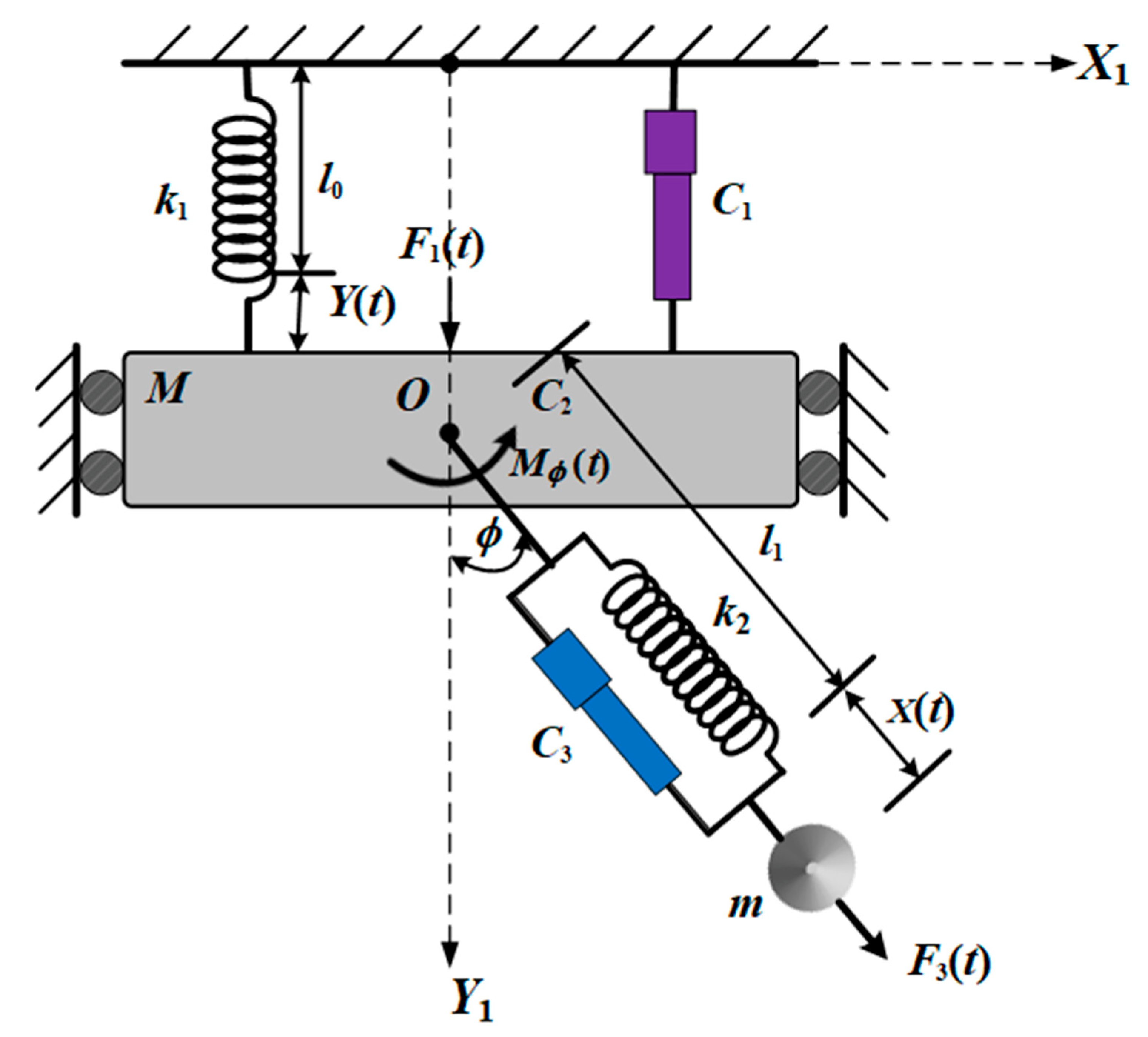
Let us consider the dynamical vibrations of an auto-parametric system consisting of an excited Duffing oscillator with normal length ${\ell }_0$, static elongation $Y_s$, stiffness $k_1$, and mass $M$ that is periodically forced to move vertically as a primary system. The secondary system is a damped spring pendulum with normal length ${\ell }_1$, static elongation $X_s$, stiffness $k_2$, and mass $m$. This spring is connected to the Duffing oscillator at a point $O$. Let $Y(t)$ denote the elongation of the Duffing oscillator and $\varphi$ represent the rotation angle of the spring that lies between the downward vertical $Y_1$-axis and the direction of the spring’s elongation $X(t)$ (see Figure 1).

Moreover, we consider that the motion is influenced by external linear excitation forces, $F_1(t)=F_1\cos ({\mathrm{\Omega }}_{1}t)$ and $F_3(t)=F_3\cos ({\mathrm{\Omega }}_{3}t)$, and an excitation moment $M_{\varphi }(t)=F_2\cos ({\mathrm{\Omega }}_{2}t)$ that are acting on the masses $M,$ $m$ and at the point $O$, respectively. Here, ${\mathrm{\Omega }}_1,\hspace{0.17em}\hspace{0.17em}{\mathrm{\Omega }}_2$, and ${\mathrm{\Omega }}_3$ are the frequencies of $F_1(t),M_{\varphi }(t)$, and $F_3(t)$, respectively. The investigated auto-parametric system is damped by viscous forces and moments $C_1\dot{Y},\hspace{0.17em}\hspace{0.17em}{C}_2\dot{\varphi }$, and $C_3\dot{X}$, in which $C_1,\hspace{0.17em}{C}_2$, and $C_3$ are the respective coefficients of the viscous damping.

Based on the above description, we can write the potential energy $V$ and kinetic energy $T$ as follows:

$$\begin{array}{l}V=\frac{1}{2}{k}_1{Y}^2+\frac{1}{2}{k}_2{X}^2-Mg(l_0+Y)-mg(l_0+Y)-mg(l_1+X)\cos \varphi ,\\ T=\frac{1}{2}(M+m){\dot{Y}}^2+\frac{1}{2}m(l_1+X)2{\dot{\varphi }}^2+\frac{1}{2}m{\dot{X}}^2\\ \hspace{0.17em}\hspace{0.17em}\hspace{0.17em}\hspace{0.17em}-m(l_1+X)\dot{Y}\dot{\varphi }\sin \varphi +m\dot{X}\dot{Y}\cos \varphi ,\end{array}$$

(1)

where $g$ is the acceleration of Earth’s gravitational force and the dots are time derivatives.

The governing EOM can be derived using the following Lagrange’s Equations:

$$\begin{array}{l}\frac{d}{dt}(\frac{\partial L}{\partial \dot{Y}})-(\frac{\partial L}{\partial Y})=Q_Y,\\ \frac{d}{dt}(\frac{\partial L}{\partial \dot{\varphi }})-(\frac{\partial L}{\partial \varphi })=Q_{\varphi },\\ \frac{d}{dt}(\frac{\partial L}{\partial \dot{X}})-(\frac{\partial L}{\partial X})=Q_X.\end{array}$$

(2)

Here, $L=T-V$ is the Lagrange’s function, $(Y,\hspace{0.17em}\varphi ,X)$ and $(\dot{Y},\hspace{0.17em}\dot{\varphi },\dot{X})$ are the system’s generalized coordinates and their corresponding velocities, respectively, and $(Q_Y,\hspace{0.17em}{Q}_{\varphi },Q_X)$ are the generalized forces which are formed as follows:

$$\begin{array}{l}{Q}_Y=F_1\cos ({\mathrm{\Omega }}_{1}t)-C_1\dot{Y},\\ Q_{\varphi }=F_2\cos ({\mathrm{\Omega }}_{2}t)-C_2\dot{\varphi },\\ Q_X=F_3\cos ({\mathrm{\Omega }}_{3}t)-C_3\dot{X}.\end{array}$$

(3)

Consider the following definitions of the dimensionless parameters:

$$\begin{array}{l}{{\overline{\omega }}_1}^2=\frac{k_1}{m+M},{{\overline{\omega }}_2}^2=\frac{g}{l_1},{{\overline{\omega }}_3}^2=\frac{k_2}{m},{{\omega }_1}^2=\frac{{{\overline{\omega }}_1}^2}{{{\overline{\omega }}_2}^2},\\ {{\omega }_2}^2=\frac{{{\overline{\omega }}_3}^2}{{{\overline{\omega }}_2}^2},c_1=\frac{C_1}{(m+M){\overline{\omega }}_2},c_2=\frac{C_2}{m{l_1}^2{\overline{\omega }}_2},c_3=\frac{C_3}{m{\overline{\omega }}_2},\\ f_1=\frac{F_1}{(m+M)l_1{{\overline{\omega }}_2}^2},f_2=\frac{F_2}{m{l_1}^2{{\overline{\omega }}_2}^2},f_3=\frac{F_3}{m{l}_1{{\overline{\omega }}_2}^2},\\ p_1=\frac{{\mathrm{\Omega }}_1}{{\overline{\omega }}_2},p_2=\frac{{\mathrm{\Omega }}_2}{{\overline{\omega }}_2},p_3=\frac{{\mathrm{\Omega }}_3}{{\overline{\omega }}_2},\beta =\frac{m}{m+M},\\ \tau ={\omega }_{2}t,x=\frac{X-X_s}{l_1},y=\frac{Y-Y_s}{l_1},Y_s=\frac{(m+M)g}{k_1},X_s=\frac{mg}{k_2},l_0={\ell }_0+Y_s,\\ l_1={\ell }_1+X_s.\end{array}$$

(4)

The substitution of Equations (1), (3) and (4) into the system of Equation (2) produces the following dimensionless form of the EOM:

$$\begin{array}{l}\ddot{y}(\tau )+{\omega }_1^{2}y-2\beta \dot{x}(\tau )\dot{\varphi }(\tau )\sin \varphi -\beta (1+x){\dot{\varphi }}^2(\tau )\cos \varphi \\ +\beta \ddot{x}(\tau )\cos \varphi -\beta (1+x)\ddot{\varphi }(\tau )\sin \varphi +c_1\dot{y}(\tau )-2=f_1\cos ({\mathrm{\Omega }}_1\tau ),\end{array}$$

(5)

$$\begin{array}{l}(1+x{)}^2\ddot{\varphi }(\tau )-(1+x)\ddot{y}(\tau )\sin \varphi +2\dot{x}(\tau )\dot{\varphi }(\tau )\\ +2x\dot{x}(\tau )\dot{\varphi }(\tau )+(1+x)\sin \varphi +c_2\dot{\varphi }(\tau )=f_2\cos ({\mathrm{\Omega }}_2\tau ),\end{array}$$

(6)

$$\begin{array}{l}\ddot{x}(\tau )+{\omega }_2^{2}x+(1+x){\dot{\varphi }}^2(\tau )+\ddot{y}(\tau )\cos \varphi -\cos \varphi \\ +c_3\dot{x}(\tau )+1=f_3\cos ({\mathrm{\Omega }}_3\tau ).\end{array}$$

(7)

The inspection of the system of Equations (5)–(7) shows that the governing EOM consists of three non-linear ordinary differential equations (ODE) in terms of $y,\varphi$, and $x$.

3. The Perturbation Technique

The main objective of the present section is to obtain the approximate analytic solutions of the EOM (5)–(7) using the PTMS to address the cases of resonance, obtain the conditions of solvability, and achieve the equations of the modulations. Therefore, we can approximate the functions $\sin \varphi$ and $\cos \varphi$ in Equations (5)–(7) using a Taylor series according to their first terms, for which these approximations are valid in a small neighborhood of the position of static equilibrium [33]. Then, Equations (5)–(7) become:

$$\begin{array}{l}\ddot{y}(\tau )+{\omega }_1^{2}y-2\beta \dot{x}(\tau )\dot{\varphi }(\tau )(\varphi -\frac{{\varphi }^3}{6})-\beta (1+x){\dot{\varphi }}^2(\tau )(1-\frac{{\varphi }^2}{2})\\ +\beta \ddot{x}(\tau )(1-\frac{{\varphi }^2}{2})-\beta (1+x)\ddot{\varphi }(\tau )(\varphi -\frac{{\varphi }^3}{6})+c_1\dot{y}(\tau )-2=f_1\cos ({\mathrm{\Omega }}_1\tau ),\end{array}$$

(8)

$$\begin{array}{l}(1+x{)}^2\ddot{\varphi }(\tau )-(1+x)\ddot{y}(\tau )(\varphi -\frac{{\varphi }^3}{6})+2\dot{x}(\tau )\dot{\varphi }(\tau )+2x\dot{x}(\tau )\dot{\varphi }(\tau )\\ +(1+x)(\varphi -\frac{{\varphi }^3}{6})+c_2\dot{\varphi }(\tau )=f_2\cos ({\mathrm{\Omega }}_2\tau ),\end{array}$$

(9)

$$\ddot{x}(\tau )+{\omega }_2^{2}x+(1+x){\dot{\varphi }}^2(\tau )+(1-\frac{{\varphi }^2}{2})\ddot{y}(\tau )+\frac{{\varphi }^2}{2}+c_3\dot{x}(\tau )=f_3\cos ({\mathrm{\Omega }}_3\tau ).$$

(10)

Based on the motion in a small neighborhood of the static equilibrium position, we consider a small parameter $0<\epsilon <<1$, in which the parameters $y,\varphi$, and $x$ can be rewritten in terms of new variables, $\xi ,\phi$, and $\chi$, respectively, according to the following forms:

$$y(\tau )=\epsilon \hspace{0.17em}\xi (\tau ;\epsilon ),\hspace{0.17em}\hspace{0.17em}\hspace{0.17em}\hspace{0.17em}\hspace{0.17em}\hspace{0.17em}\hspace{0.17em}\hspace{0.17em}\hspace{0.17em}\hspace{0.17em}\hspace{0.17em}\hspace{0.17em}\hspace{0.17em}\hspace{0.17em}\varphi (\tau )=\epsilon \hspace{0.17em}\phi (\tau ;\epsilon ),\hspace{0.17em}\hspace{0.17em}\hspace{0.17em}\hspace{0.17em}\hspace{0.17em}\hspace{0.17em}\hspace{0.17em}\hspace{0.17em}\hspace{0.17em}\hspace{0.17em}\hspace{0.17em}\hspace{0.17em}\hspace{0.17em}\hspace{0.17em}x(\tau )=\epsilon \hspace{0.17em}\chi (\tau ;\epsilon ).$$

(11)

According to PTMS, we can seek the approximate solutions of the variables $\xi ,\phi$, and $\chi$ in the following forms [34]:

$$\begin{array}{l}\xi ={\displaystyle \sum _{k=0}^2{\epsilon }^k{\xi }_{k+1}({\tau }_0,{\tau }_1,{\tau }_2)+}O({\epsilon }^3),\\ \phi ={\displaystyle \sum _{k=0}^2{\epsilon }^k{\phi }_{k+1}({\tau }_0,{\tau }_1,{\tau }_2)}+O({\epsilon }^3),\\ \chi ={\displaystyle \sum _{k=0}^2{\epsilon }^k{\chi }_{k+1}({\tau }_0,{\tau }_1,{\tau }_2)}+O({\epsilon }^3),\end{array}$$

(12)

where ${\tau }_n={\epsilon }^n\tau \hspace{0.17em}\hspace{0.17em}(n=0,\hspace{0.17em}1,\hspace{0.17em}2)$ are various time scales, in which ${\tau }_0$ and ${\tau }_1,{\tau }_2$ are defined as fast and slow time scales, respectively. Therefore, the time derivatives regarding $\tau$ can be transformed according to the time scales ${\tau }_n$ as the following chain rule:

$$\begin{array}{l}\frac{d}{d\tau }=\frac{\partial }{\partial {\tau }_0}+\epsilon \frac{\partial }{\partial {\tau }_1}+{\epsilon }^2\frac{\partial }{\partial {\tau }_2}+O({\epsilon }^3),\\ \frac{d^2}{d{\tau }^2}=\frac{{\partial }^2}{\partial {\tau }_0^2}+2\epsilon \frac{{\partial }^2}{\partial {\tau }_0\partial {\tau }_1}+{\epsilon }^2(\frac{{\partial }^2}{\partial {\tau }_1^2}+2\frac{{\partial }^2}{\partial {\tau }_0\partial {\tau }_2})+O({\epsilon }^3),\end{array}$$

(13)

where terms of $O({\epsilon }^3)$ and higher are neglected due to their minuteness.

As before, we consider the minuteness of the amplitudes of external forces and moments $f_j\hspace{0.17em}\hspace{0.17em}(j=1,2,3)$, as well as the coefficients of damping $c_i$. Therefore, we can write:

$$f_j={\epsilon }^3{\tilde{f}}_j,\hspace{0.17em}\hspace{0.17em}\hspace{0.17em}\hspace{0.17em}\hspace{0.17em}\hspace{0.17em}\hspace{0.17em}\hspace{0.17em}\hspace{0.17em}{c}_j={\epsilon }^2{\tilde{c}}_j\hspace{0.17em}\hspace{0.17em}\hspace{0.17em}\hspace{0.17em}\hspace{0.17em}\hspace{0.17em}\hspace{0.17em}\hspace{0.17em}\hspace{0.17em}\hspace{0.17em}\hspace{0.17em}\hspace{0.17em}\hspace{0.17em}(j=1,2,3).$$

(14)

Furthermore, we consider the following:

$$\beta =\epsilon \tilde{\beta },$$

(15)

where the amounts ${\tilde{f}}_j,{\tilde{c}}_j,\tilde{a},\tilde{b}$, and $\tilde{\beta }$ are of order unity.

Substituting the new variables into Equations of system (11), the assumed solutions (12), the transformations (13), and the use of the parameters of Equations (14) and (15) into the EOM (8)–(10) and equating the coefficients of like powers of $\epsilon$ in each side obtains the following groups of partial differential equations (PDEs):

Equations of order$\epsilon$:

$$\frac{{\partial }^2{\xi }_1}{\partial {\tau }_0^2}+{\omega }_1^2{\xi }_1=0,$$

(16)

$$\frac{{\partial }^2{\phi }_1}{\partial {\tau }_0^2}+{\phi }_1=0,$$

(17)

$$\frac{{\partial }^2{\chi }_1}{\partial {\tau }_0^2}+{\omega }_2^2{\chi }_1+\frac{{\partial }^2{\xi }_1}{\partial {\tau }_0^2}=0.$$

(18)

Equations of order${\epsilon }^2$:

$$\frac{{\partial }^2{\xi }_2}{\partial {\tau }_0^2}+{\omega }_1^2{\xi }_2=-2\frac{{\partial }^2{\xi }_1}{\partial {\tau }_0{\tau }_1}-\tilde{\beta }\frac{{\partial }^2{\chi }_1}{\partial {\tau }_0^2},$$

(19)

$$\frac{{\partial }^2{\varphi }_2}{\partial {\tau }_0^2}+{\varphi }_2=-2\frac{{\partial }^2{\varphi }_1}{\partial {\tau }_0\partial {\tau }_1}-2{\chi }_1\frac{{\partial }^2{\varphi }_1}{\partial {\tau }_0^2}+{\varphi }_1\frac{{\partial }^2{\xi }_1}{\partial {\tau }_0^2}-2\frac{\partial {\varphi }_1}{\partial {\tau }_0}\frac{\partial {\chi }_1}{\partial {\tau }_0}-{\varphi }_1{\chi }_1,$$

(20)

$$\frac{{\partial }^2{\chi }_2}{\partial {\tau }_0^2}+{\omega }_2^2{\chi }_2+\frac{{\partial }^2{\xi }_2}{\partial {\tau }_0^2}=-2\frac{{\partial }^2{\chi }_1}{\partial {\tau }_0\partial {\tau }_1}-\frac{3}{2}{\varphi }_1{}^2-2\frac{{\partial }^2{\xi }_1}{\partial {\tau }_0\partial {\tau }_1}.$$

(21)

Equations of order${\epsilon }^3$:

$$\begin{array}{l}\frac{{\partial }^2{\xi }_3}{\partial {\tau }_0^2}+{\omega }_1^2{\xi }_3=-\frac{{\partial }^2{\xi }_1}{\partial {\tau }_0^2}-2\frac{{\partial }^2{\xi }_1}{\partial {\tau }_0\partial {\tau }_2}-2\frac{{\partial }^2{\xi }_2}{\partial {\tau }_0\partial {\tau }_1}+\tilde{\beta }(\frac{\partial {\varphi }_1}{\partial {\tau }_0}{)}^2-2\tilde{\beta }\frac{{\partial }^2{\chi }_1}{\partial {\tau }_0\partial {\tau }_1}\\ \hspace{0.17em}\hspace{0.17em}\hspace{0.17em}\hspace{0.17em}\hspace{0.17em}\hspace{0.17em}\hspace{0.17em}\hspace{0.17em}\hspace{0.17em}\hspace{0.17em}\hspace{0.17em}\hspace{0.17em}\hspace{0.17em}\hspace{0.17em}\hspace{0.17em}\hspace{0.17em}\hspace{0.17em}\hspace{0.17em}\hspace{0.17em}\hspace{0.17em}\hspace{0.17em}\hspace{0.17em}\hspace{0.17em}\hspace{0.17em}\hspace{0.17em}-\tilde{\beta }\frac{{\partial }^2{\chi }_2}{\partial {\tau }_0^2}+\tilde{\beta }{\varphi }_1\frac{{\partial }^2{\varphi }_1}{\partial {\tau }_0^2}-{\tilde{c}}_1\frac{\partial {\xi }_1}{\partial {\tau }_0}+{\tilde{f}}_1\cos (p_1{\tau }_0),\end{array}$$

(22)

$$\begin{array}{l}\frac{{\partial }^2{\varphi }_3}{\partial {\tau }_0^2}+{\varphi }_3=-\frac{{\partial }^2{\varphi }_1}{\partial {\tau }_1^2}-2\frac{{\partial }^2{\varphi }_1}{\partial {\tau }_0\partial {\tau }_2}-2\frac{{\partial }^2{\varphi }_2}{\partial {\tau }_0\partial {\tau }_1}-4{\chi }_1\frac{{\partial }^2{\varphi }_1}{\partial {\tau }_0\partial {\tau }_1}-2{\chi }_1\frac{{\partial }^2{\varphi }_2}{\partial {\tau }_0^2}-2{\chi }_2\frac{{\partial }^2{\varphi }_1}{\partial {\tau }_0^2}\\ \hspace{0.17em}\hspace{0.17em}\hspace{0.17em}\hspace{0.17em}\hspace{0.17em}\hspace{0.17em}\hspace{0.17em}\hspace{0.17em}\hspace{0.17em}\hspace{0.17em}\hspace{0.17em}\hspace{0.17em}\hspace{0.17em}-{{\chi }_1}^2\frac{{\partial }^2{\varphi }_1}{\partial {\tau }_0^2}+2{\varphi }_1\frac{{\partial }^2{\xi }_1}{\partial {\tau }_0\partial {\tau }_1}+{\varphi }_2\frac{{\partial }^2{\xi }_1}{\partial {\tau }_0^2}+{\varphi }_1\frac{{\partial }^2{\xi }_2}{\partial {\tau }_0^2}-2\frac{\partial {\varphi }_1}{\partial {\tau }_1}\frac{\partial {\chi }_1}{\partial {\tau }_0}-2\frac{\partial {\varphi }_1}{\partial {\tau }_0}\frac{\partial {\chi }_1}{\partial {\tau }_1}\\ \hspace{0.17em}\hspace{0.17em}\hspace{0.17em}\hspace{0.17em}\hspace{0.17em}\hspace{0.17em}\hspace{0.17em}\hspace{0.17em}\hspace{0.17em}\hspace{0.17em}\hspace{0.17em}\hspace{0.17em}\hspace{0.17em}-2\frac{\partial {\varphi }_2}{\partial {\tau }_1}\frac{\partial {\chi }_1}{\partial {\tau }_0}-2\frac{\partial {\varphi }_1}{\partial {\tau }_0}\frac{\partial {\chi }_2}{\partial {\tau }_0}-2{\chi }_1\frac{\partial {\varphi }_1}{\partial {\tau }_0}\frac{\partial {\chi }_1}{\partial {\tau }_0}-{\chi }_1{\varphi }_2-{\chi }_2{\varphi }_2+\frac{{{\varphi }_1}^3}{6}-{\tilde{c}}_2\frac{\partial {\varphi }_1}{\partial {\tau }_0}\\ \hspace{0.17em}\hspace{0.17em}\hspace{0.17em}\hspace{0.17em}\hspace{0.17em}\hspace{0.17em}\hspace{0.17em}\hspace{0.17em}\hspace{0.17em}\hspace{0.17em}\hspace{0.17em}\hspace{0.17em}\hspace{0.17em}+{\tilde{f}}_{2}cos\left(p_2{\tau }_0\right),\end{array}$$

(23)

$$\begin{array}{ll}\hfill \frac{{\partial }^2{\chi }_3}{\partial {\tau }_0^2}& +{\omega }_2^2{\chi }_3+\frac{{\partial }^2{\xi }_3}{\partial {\tau }_0^2}=-\frac{{\partial }^2{\chi }_1}{\partial {\tau }_1^2}-2\frac{{\partial }^2{\chi }_1}{\partial {\tau }_0\partial {\tau }_2}-2\frac{{\partial }^2{\chi }_2}{\partial {\tau }_0\partial {\tau }_1}-2\frac{\partial {\varphi }_1}{\partial {\tau }_0}\frac{\partial {\varphi }_2}{\partial {\tau }_0}-{\chi }_1(\frac{\partial {\varphi }_1}{\partial {\tau }_0}{)}^2\hfill \\ & -\frac{{\partial }^2{\xi }_1}{\partial {\tau }_1^2}-2\frac{{\partial }^2{\xi }_1}{\partial {\tau }_0\partial {\tau }_2}-2\frac{{\partial }^2{\xi }_2}{\partial {\tau }_0\partial {\tau }_1}+\frac{3}{2}{\varphi }_1{}^2\frac{{\partial }^2{\xi }_1}{\partial {\tau }_0^2}-{\varphi }_1{\varphi }_2-{\tilde{c}}_3\frac{\partial {\chi }_1}{\partial {\tau }_0}+{\tilde{f}}_3\cos (p_3{\tau }_0).\hfill \end{array}$$

(24)

The above nine PDE (16)–(24) can be solved sequentially one by one. Consequently, the general solutions of Equations (16) and (17) are:

$${\xi }_1={\mathrm{A}}_1{e}^{i{\omega }_1{\tau }_0}+{\overline{\mathrm{A}}}_1{e}^{-i{\omega }_1{\tau }_0},$$

(25)

$${\varphi }_1\hspace{0.17em}={\mathrm{A}}_2{e}^{i\hspace{0.17em}{\tau }_0}+{\overline{\mathrm{A}}}_2{e}^{-i\hspace{0.17em}{\tau }_0}.$$

(26)

The substitution of Equation (25) into Equation (18) yields a nonhomogeneous equation, and its solution can be written in the form:

$${\chi }_1={\mathrm{A}}_3{e}^{i{\omega }_2{\tau }_0}+{\overline{\mathrm{A}}}_3{e}^{-i{\omega }_2{\tau }_0}+\frac{{\omega }_1^2}{{\omega }_1^2-{\omega }_2^2}({\mathrm{A}}_1{e}^{i{\omega }_1{\tau }_0}+{\overline{\mathrm{A}}}_1{e}^{-i{\omega }_1{\tau }_0}),$$

(27)

where ${\mathrm{A}}_j\hspace{0.17em}\hspace{0.17em}(j=1,\hspace{0.17em}2,\hspace{0.17em}3)$ represent unknown complex functions of the slow time scales ${\tau }_1,{\tau }_2$, while ${\overline{\mathrm{A}}}_j$ are the complex conjugates of these functions.

The substitution of the first-order solutions of Equations (25)–(27) into Equations (19)–(21) yields secular terms. The elimination of these terms demands that:

$$2i{\omega }_1\frac{\partial {\mathrm{A}}_1}{\partial {\tau }_1}-\frac{\tilde{\beta }{\omega }_1^4}{({\omega }_1^2-{\omega }_2^2)}{\mathrm{A}}_1=0,$$

(28)

$$\frac{\partial {\mathrm{A}}_2}{\partial {\tau }_1}=0.$$

(29)

According to these conditions, the second-order solutions have the following forms:

$${\xi }_2=\frac{\tilde{\beta }{\omega }_2^2}{({\omega }_1^2-{\omega }_2^2)}{\mathrm{A}}_3{e}^{i{\omega }_2{\tau }_0}+CC.,$$

(30)

$$\begin{array}{l}{\varphi }_2=-\frac{{\omega }_1{\mathrm{A}}_2}{({\omega }_1^2-{\omega }_2^2)}\{\frac{[(1+2{\omega }_1)-({\omega }_1^2-{\omega }_2^2)]}{({\omega }_1+2)}{\mathrm{A}}_1{e}^{i(1+{\omega }_1){\tau }_0}+\frac{[(1-2{\omega }_1)-({\omega }_1^2-{\omega }_2^2)]}{({\omega }_1-2)}\\ \hspace{0.17em}\hspace{0.17em}\hspace{0.17em}\hspace{0.17em}\hspace{0.17em}\hspace{0.17em}\times {\overline{\mathrm{A}}}_1{e}^{i(1-{\omega }_1){\tau }_0}\}-\frac{{\mathrm{A}}_2}{{\omega }_2}[\frac{(1+2{\omega }_2)}{({\omega }_2+2)}{\mathrm{A}}_3{e}^{i(1+{\omega }_2){\tau }_0}+\frac{(1-2{\omega }_2)}{({\omega }_2-2)}{\overline{\mathrm{A}}}_3{e}^{i(1-{\omega }_2){\tau }_0}]+CC.\hspace{0.17em}\end{array}$$

(31)

Here, $CC.$ represents the complex conjugates of the preceding terms.

After grasping the above procedure, we can obtain another condition for eliminating the secular terms by substituting the solutions from Equations (25)–(27), (30) and (31) into Equation (21), in the following form:

$$2i{\omega }_2\frac{\partial {\mathrm{A}}_3}{\partial {\tau }_1}-\frac{\tilde{\beta }\hspace{0.17em}{\omega }_2^4}{{\omega }_1^2-{\omega }_2^2}{\mathrm{A}}_3=0.$$

(32)

Therefore, the solution ${\chi }_2$ has the form:

$${\chi }_2=-\frac{3{\mathrm{A}}_2{\overline{\mathrm{A}}}_2}{{\omega }_2^2}\hspace{0.17em}-\frac{3\hspace{0.17em}{\mathrm{A}}_2^2}{2({\omega }_2^4-4)}\hspace{0.17em}{e}^{2i\hspace{0.17em}{\tau }_0}+\frac{\tilde{\beta }\hspace{0.17em}{\omega }_1^4{\omega }_2^2}{{({\omega }_1^2-{\omega }_2^2)}^3}\hspace{0.17em}{\mathrm{A}}_1{e}^{i{\omega }_1{\tau }_0}+CC.$$

(33)

Making use of the previous solutions to Equations (25)–(27), (30), (31) and (33) and the third-order approximate Equations (22)–(24), secular terms are produced. The eliminating conditions of these terms required that:

$$2i{\omega }_1\frac{\partial {\mathrm{A}}_1}{\partial {\tau }_2}\hspace{0.17em}\hspace{0.17em}+\hspace{0.17em}i{\omega }_1{\tilde{c}}_1{\mathrm{A}}_1-\frac{{\tilde{\beta }}^2{\omega }_1^6{\mathrm{A}}_1}{4{({\omega }_1^2-{\omega }_2^2)}^3}[-{\omega }_1^2(4{\omega }_1^2+11)+{\omega }_2^2(7-4{\omega }_2^2)+8{\omega }_1^2{\omega }_2^2]\hspace{0.17em}\hspace{0.17em}=0,\hspace{0.17em}$$

(34)

$$\begin{array}{l}2i\frac{\partial {\mathrm{A}}_2}{\partial {\tau }_2}\hspace{0.17em}\hspace{0.17em}+\hspace{0.17em}i\hspace{0.17em}{\tilde{c}}_2{\mathrm{A}}_2-\frac{6{\omega }_1^4({\omega }_2^2-2{\omega }_1^2+1)}{({\omega }_1^2-4){({\omega }_1^2-{\omega }_2^2)}^2}{\mathrm{A}}_1{\mathrm{A}}_2{\overline{\mathrm{A}}}_1-\frac{{\mathrm{A}}_2^2{\overline{\mathrm{A}}}_2}{2{\omega }_2^2({\omega }_2^2-4)}({\omega }_2^4-25{\omega }_2^2+24)\\ -\frac{{\mathrm{A}}_2{\mathrm{A}}_3{\overline{\mathrm{A}}}_3}{({\omega }_2^2-4)({\omega }_2^2-{\omega }_1^2)}\{6{\omega }_1^2({\omega }_2^2-1)+{\omega }_2^2[6(1-{\omega }_2^2)+\tilde{\beta }{\omega }_2(2{\omega }_2^2+3{\omega }_2-2)]\}=0,\end{array}$$

(35)

$$2i{\omega }_2\frac{\partial {\mathrm{A}}_3}{\partial {\tau }_2}\hspace{0.17em}\hspace{0.17em}+\hspace{0.17em}i\hspace{0.17em}{\tilde{c}}_3{\omega }_2{\mathrm{A}}_3+\frac{{\tilde{\beta }}^2{\omega }_2^6{\mathrm{A}}_3}{2{({\omega }_1^2-{\omega }_2^2)}^2}(1-2\hspace{0.17em}{\omega }_1^2)-\frac{3+2{\omega }_2({\omega }_2+2)}{{\omega }_2({\omega }_2+2)}{\mathrm{A}}_2{\mathrm{A}}_3{\overline{\mathrm{A}}}_2=0.$$

(36)

Based on the previous conditions of Equations (34)–(36), the approximate third-order solutions turn into:

$$\begin{array}{l}{\xi }_3=\frac{{\tilde{f}}_1{e}^{i{p}_1{\tau }_0}}{2({\omega }_1^2-p_1{}^2)}-\frac{[2\tilde{\beta }\hspace{0.17em}{\mathrm{A}}_2^2\hspace{0.17em}({\omega }_2^2-4)+6\tilde{\beta }\hspace{0.17em}{\mathrm{A}}_2^2]}{({\omega }_1^2-4)({\omega }_2^2-4)}{e}^{2i\hspace{0.17em}{\tau }_0}\\ \hspace{0.17em}\hspace{0.17em}\hspace{0.17em}\hspace{0.17em}\hspace{0.17em}\hspace{0.17em}-[\frac{1}{{({\omega }_1^2-{\omega }_2^2)}^2}+\frac{{\omega }_2^2\hspace{0.17em}}{{({\omega }_1^2-{\omega }_2^2)}^3}]{\tilde{\beta }}^2\hspace{0.17em}{\omega }_2^4\hspace{0.17em}{\mathrm{A}}_3{e}^{i\hspace{0.17em}{\omega }_2\hspace{0.17em}{\tau }_0}+CC\hspace{0.17em}\hspace{0.17em},\end{array}$$

(37)

$$\begin{array}{cc}\hfill {\varphi }_3& =\frac{{\tilde{f}}_2{e}^{i{p}_2{\tau }_0}}{2(1-p_2{}^2)}+{\overline{\mathrm{A}}}_3{\mathrm{A}}_2[\frac{d_1}{d_2\hspace{0.17em}}{\overline{\mathrm{A}}}_1{e}^{i(1-{\omega }_1-{\omega }_2){\tau }_0}\hspace{0.17em}+\frac{d_3}{d_4\hspace{0.17em}}{\mathrm{A}}_1{e}^{i(1+{\omega }_1-{\omega }_2){\tau }_0}]+{\mathrm{A}}_2\{\frac{d_5}{d_6\hspace{0.17em}}{\mathrm{A}}_1^2{e}^{i(1+2{\omega }_1){\tau }_0}\\ & +{\mathrm{A}}_3[\frac{d_7}{d_8\hspace{0.17em}}{\overline{\mathrm{A}}}_1{e}^{i(1-{\omega }_1+{\omega }_2){\tau }_0}+\frac{d_9}{d_{10}\hspace{0.17em}}{\mathrm{A}}_1{e}^{i(1+{\omega }_1+{\omega }_2){\tau }_0}]\}+CC\hspace{0.17em}\hspace{0.17em},\end{array}$$

(38)

$$\begin{array}{cc}\hfill {\chi }_3& =\frac{{\tilde{f}}_1{p_1}^2{e}^{i{p}_1{\tau }_0}}{2({\omega }_1^2-{p_1}^2)({\omega }_2^2-{p_1}^2)}+\frac{{\tilde{f}}_3{e}^{i{p}_3{\tau }_0}}{2({\omega }_2^2-{p_3}^2)}+\frac{d_{11}}{d_{12}}{\mathrm{A}}_1{\mathrm{A}}_2{\overline{\mathrm{A}}}_2{e}^{i{\omega }_1{\tau }_0}\hfill \\ & +{\mathrm{A}}_2^2[\frac{d_{13}}{d_{14}}{\overline{\mathrm{A}}}_1{e}^{i(2-{\omega }_1){\tau }_0}+\frac{d_{15}}{d_{16}}{\mathrm{A}}_1{e}^{i(2+{\omega }_1){\tau }_0}+\frac{d_{17}}{d_{18}}{\overline{\mathrm{A}}}_3{e}^{i(2-{\omega }_2){\tau }_0}\hfill \\ & +\frac{d_{19}}{d_{20}}{\mathrm{A}}_3{e}^{i(2+{\omega }_2){\tau }_0}-\frac{8\tilde{\beta }({\omega }_2^2-1)}{({\omega }_1^2-4)({\omega }_2^2-4)}{e}^{2i{\tau }_0}]+CC.,\hfill \end{array}$$

(39)

where $d_s\hspace{0.17em}\hspace{0.17em}(s=1,2,3,\dots ,20)$ are functions of ${\omega }_1$ and ${\omega }_2$ (see Appendix A).

According to the removal conditions of secular terms, Equations (34)–(36), and the following initial conditions, we can estimate the functions ${\mathrm{A}}_j\hspace{0.17em}\hspace{0.17em}(j=1,\hspace{0.17em}2,\hspace{0.17em}3)$:

$$\begin{array}{l}y(0)=B_{01},\hspace{0.17em}\hspace{0.17em}\hspace{0.17em}\hspace{0.17em}\hspace{0.17em}\hspace{0.17em}\hspace{0.17em}\hspace{0.17em}\dot{y}(0)=B_{02},\hspace{0.17em}\hspace{0.17em}\hspace{0.17em}\hspace{0.17em}\hspace{0.17em}\hspace{0.17em}\hspace{0.17em}\hspace{0.17em}\varphi (0)=B_{03},\\ \dot{\varphi }(0)=B_{04},\hspace{0.17em}\hspace{0.17em}\hspace{0.17em}\hspace{0.17em}\hspace{0.17em}\hspace{0.17em}\hspace{0.17em}\hspace{0.17em}x(0)=B_{05},\hspace{0.17em}\hspace{0.17em}\hspace{0.17em}\hspace{0.17em}\hspace{0.17em}\hspace{0.17em}\hspace{0.17em}\hspace{0.17em}\dot{x}(0)=B_{06},\end{array}$$

(40)

where $B_{0k}(k=1,2,\dots ,6)$ are known values.

Now, we will investigate the arising cases of resonance according to the previous approximate solutions. These cases can be categorized into primary (main) external resonance, which takes place at $p_1={\omega }_1,$ $p_2=1,$ $p_3={\omega }_2$, and internal resonance, which occurs at ${\omega }_1={\omega }_2,$ ${\omega }_1=-{\omega }_2,$ ${\omega }_1=2,$ ${\omega }_1=-2,$ ${\omega }_2=2,$ ${\omega }_2=-2$.

In this situation, we investigate the three primary external resonances, $p_1\approx {\omega }_1,\hspace{0.17em}\hspace{0.17em}{p}_2\approx 1$, and $p_3\approx {\omega }_2$, simultaneously. These resonances depict the closeness of $p_1,\hspace{0.17em}{p}_2$ and $p_3$ to ${\omega }_1,\hspace{0.17em}1$ and ${\omega }_2$, respectively. Therefore, detuning parameters ${\sigma }_j\hspace{0.17em}\hspace{0.17em}(j=1,\hspace{0.17em}2,\hspace{0.17em}3)$ can be introduced according to:

$$p_1={\omega }_1+{\sigma }_1,\hspace{0.17em}\hspace{0.17em}\hspace{0.17em}\hspace{0.17em}\hspace{0.17em}{p}_2=1+{\sigma }_2,\hspace{0.17em}\hspace{0.17em}\hspace{0.17em}\hspace{0.17em}\hspace{0.17em}\hspace{0.17em}\hspace{0.17em}{p}_3={\omega }_2+{\sigma }_3.$$

(41)

Since the detuning parameters are known as the distances from the oscillations to the strict resonance [35,36], we can use the small parameter $\epsilon$ to express these parameters as follows:

$${\sigma }_j=\epsilon {\tilde{\sigma }}_j\hspace{0.17em}\hspace{0.17em}\hspace{0.17em}\hspace{0.17em}\hspace{0.17em}\hspace{0.17em}\hspace{0.17em}\hspace{0.17em}\hspace{0.17em}\hspace{0.17em}(j=1,2,3).$$

(42)

Substituting parameters (41) and (42) into Equations (8)–(10) and removing the produced secular terms obtains the following conditions of solvability:

$$\begin{array}{l}2i{\omega }_1\frac{\partial {\mathrm{A}}_1}{\partial {\tau }_2}+i{\omega }_1{\tilde{c}}_1{\mathrm{A}}_1-\frac{{\tilde{\beta }}^2{\omega }_1^6{\mathrm{A}}_1}{4{({\omega }_1^2-{\omega }_2^2)}^3}[-{\omega }_1^2(4{\omega }_1^2+11)+{\omega }_2^2(7-4{\omega }_2^2)\\ +8{\omega }_1^2{\omega }_2^2]-\frac{{\tilde{f}}_1}{2}{e}^{i{\tilde{\sigma }}_1{\tau }_1}=0,\\ 2i\frac{\partial {\mathrm{A}}_2}{\partial {\tau }_2}+i{\tilde{c}}_2{\mathrm{A}}_2-\frac{6{\omega }_1^4({\omega }_2^2-2{\omega }_1^2+1)}{({\omega }_1^2-4){({\omega }_1^2-{\omega }_2^2)}^2}{\mathrm{A}}_1{\mathrm{A}}_2{\overline{\mathrm{A}}}_1-\frac{{\mathrm{A}}_2{\mathrm{A}}_3{\overline{\mathrm{A}}}_3}{({\omega }_2^2-4)({\omega }_2^2-{\omega }_1^2)}\\ \times \{6{\omega }_1^2({\omega }_2^2-1)+{\omega }_2^2[6(1-{\omega }_2^2)+\tilde{\beta }{\omega }_2(2{\omega }_2^2+3{\omega }_2-2)]\}-\frac{{}_2^2{\overline{\mathrm{A}}}_2}{2{\omega }_2^2({\omega }_2^2-4)}\\ \times ({\omega }_2^4-25{\omega }_2^2+24)-\frac{{\tilde{f}}_2}{2}{e}^{i{\tilde{\sigma }}_2{\tau }_1}=0,\\ 2i{\omega }_2\frac{\partial {}_3}{\partial {\tau }_2}+i{\tilde{c}}_3{\omega }_2{\mathrm{A}}_3-\frac{(2{\omega }_1^2-1)}{2{({\omega }_1^2-{\omega }_2^2)}^2}{\mathrm{A}}_3{\tilde{\beta }}^2{\omega }_2^6-\frac{[3+2{\omega }_2({\omega }_2+2)]}{{\omega }_2({\omega }_2+2)}\\ \times {\mathrm{A}}_2{\mathrm{A}}_3{\overline{\mathrm{A}}}_2-\frac{{\tilde{f}}_3}{2}{e}^{i{\tilde{\sigma }}_3{\tau }_1}=0.\end{array}$$

(43)

It is obvious that these conditions constitute a system of three non-linear PDEs in terms of the functions ${\mathrm{A}}_j\hspace{0.17em}\hspace{0.17em}(j=1,\hspace{0.17em}2,\hspace{0.17em}3)$, in which ${\mathrm{A}}_j={\mathrm{A}}_j({\tau }_1,{\tau }_2)$. Therefore, we can write them in polar forms as follows:

$${\mathrm{A}}_j=\frac{{\tilde{h}}_j({\tau }_1,{\tau }_2)}{2}{e}^{i\hspace{0.17em}{\psi }_j({\tau }_1,{\tau }_2)},\hspace{0.17em}\hspace{0.17em}\hspace{0.17em}\hspace{0.17em}\hspace{0.17em}\hspace{0.17em}\hspace{0.17em}\hspace{0.17em}\hspace{0.17em}\hspace{0.17em}{h}_j=\epsilon {\tilde{h}}_j\hspace{0.17em}\hspace{0.17em}\hspace{0.17em}\hspace{0.17em}\hspace{0.17em}\hspace{0.17em}\hspace{0.17em}\hspace{0.17em}\hspace{0.17em}(j=1,2,3).$$

(44)

Here, ${\tilde{h}}_j$ and ${\psi }_j$ are real functions of the amplitudes and phases, respectively, for the functions $\xi ,\hspace{0.17em}\phi$ and $\chi$, while $h_j$ are the amplitudes of $y,\hspace{0.17em}\hspace{0.17em}\varphi$, and $x$, as presented in the assumptions of Equations (11) and (12).

Making use of the following modified phases:

$${\theta }_j({\tau }_1,{\tau }_2)={\tau }_j{\tilde{\sigma }}_j-{\psi }_j({\tau }_1,{\tau }_2)$$

(45)

and the time derivative operators (13), we can transform the PDE system (43) into another ODE system. The separation of the real and imaginary parts of the resulting system yields the following six ODEs from the first order that describe the modulation equations in terms of modified phases ${\theta }_j$ and amplitudes $h_j$ in the following forms:

$$\begin{array}{l}{h}_1\frac{d{\theta }_1}{d\tau }=h_1{\sigma }_1+\frac{{\beta }^2{\omega }_1^5{h}_1}{4{({\omega }_1^2-{\omega }_2^2)}^3}[-{\omega }_1^2(4{\omega }_1^2+11)+{\omega }_2^2(7-4{\omega }_2^2)+8{\omega }_1^2{\omega }_2^2]+\frac{f_1}{2{\omega }_1}cos{\theta }_1,\\ \frac{d{h}_1}{d\tau }=-\frac{1}{2}{h}_1{c}_1+\frac{f_1}{2{\omega }_1}sin{\theta }_1,\\ h_2\frac{d{\theta }_2}{d\tau }=h_2{\sigma }_2-\frac{6{\omega }_1^2{h}_1^2{h}_2}{8({\omega }_1^2-4){({\omega }_1^2-{\omega }_2^2)}^2}({\omega }_2^2-2{\omega }_1^2+1)+\frac{h_2^3}{16{\omega }_2^2({\omega }_2^2-4)}\\ \times ({\omega }_2^4-25{\omega }_2^2+24)-\frac{3h_3^2{h}_2}{4({\omega }_2^2-4)}({\omega }_2^2-1)+\frac{f_2}{2}cos{\theta }_2,\\ \frac{d{h}_2}{d\tau }=-\frac{1}{2}{h}_2{c}_2+\frac{f_2}{2}sin{\theta }_2,\\ h_3\frac{d{\theta }_3}{d\tau }=h_3{\sigma }_3+\frac{{\beta }^2{\omega }_2^5{h}_3}{4{({\omega }_1^2-{\omega }_2^2)}^3}({\omega }_2^2-3{\omega }_1^2)+\frac{h_2^2{h}_3}{8{\omega }_2^2({\omega }_2+2)}[3+2{\omega }_2({\omega }_2+2)]+\frac{f_3}{2{\omega }_2}cos{\theta }_3,\\ \frac{d{h}_3}{d\tau }=-\frac{1}{2}{h}_3{c}_3+\frac{f_3}{2{\omega }_2}sin{\theta }_3.\end{array}$$

(46)

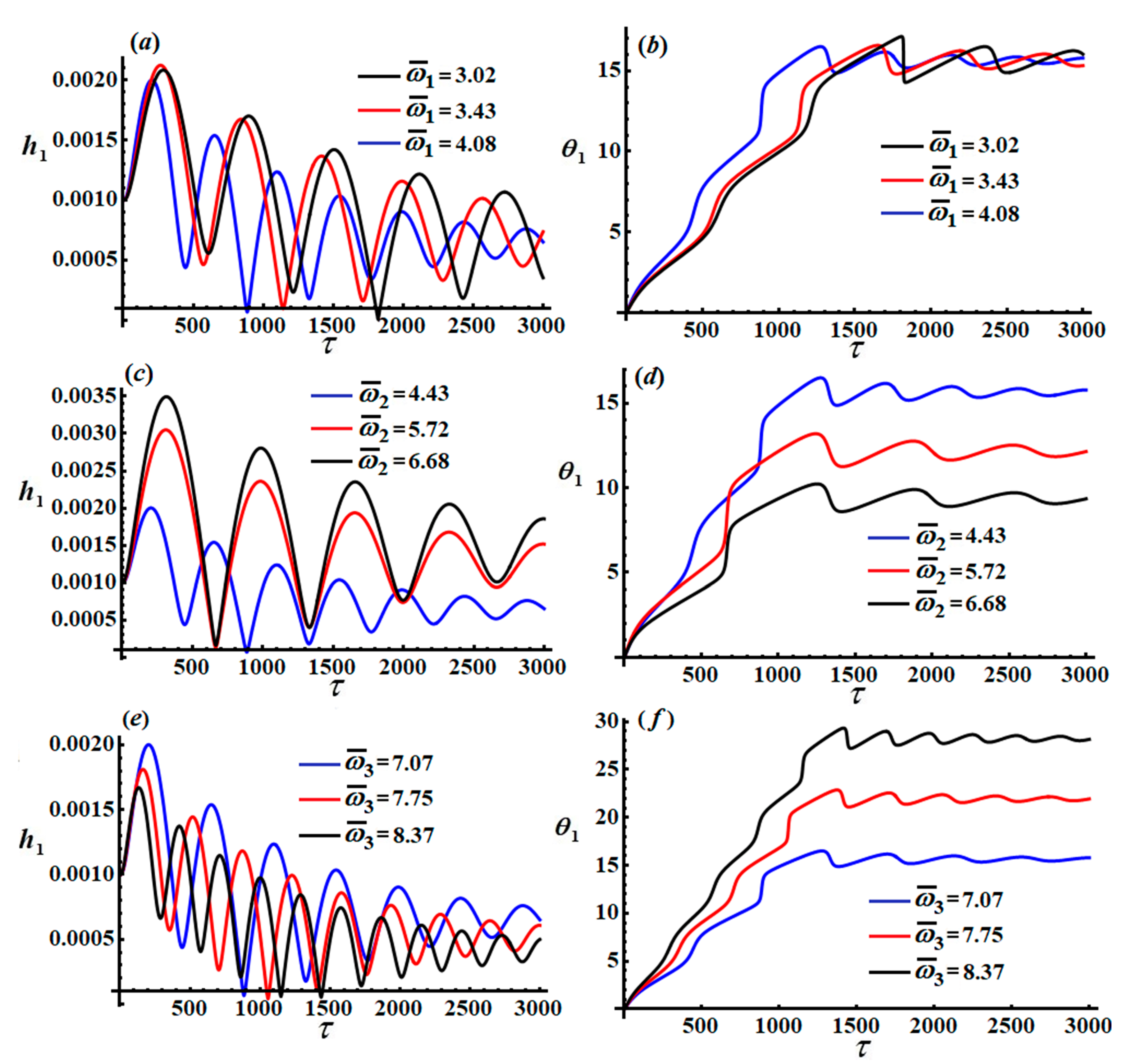
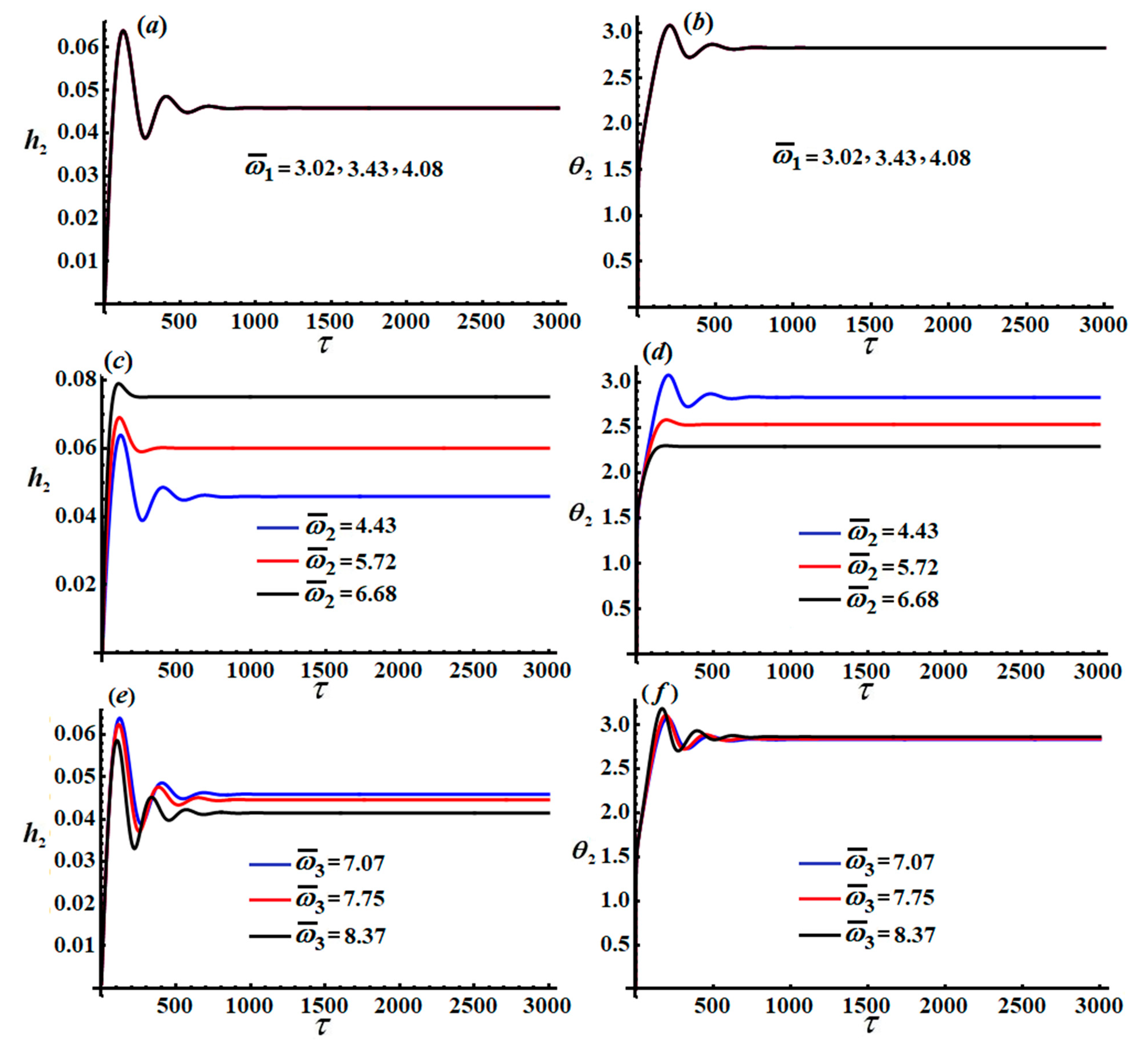
According to the conditions (40), we can solve the above modulation in Equation (46). The time histories of the amplitudes $h_j\hspace{0.17em}\hspace{0.17em}(j=1,2,3)$ and the modified phases ${\theta }_j$ are portrayed in Figure 2, Figure 3 and Figure 4, according to the uses of the following data:

$$\begin{array}{l}{\sigma }_1=0.01,\hspace{0.17em}\hspace{0.17em}\hspace{0.17em}\hspace{0.17em}\hspace{0.17em}\hspace{0.17em}\hspace{0.17em}{\sigma }_2=0.02,\hspace{0.17em}\hspace{0.17em}\hspace{0.17em}\hspace{0.17em}\hspace{0.17em}\hspace{0.17em}\hspace{0.17em}{\sigma }_3=0.03,\hspace{0.17em}\hspace{0.17em}\hspace{0.17em}\hspace{0.17em}\hspace{0.17em}\hspace{0.17em}\hspace{0.17em}{f}_1=0.00002,\hspace{0.17em}\hspace{0.17em}\hspace{0.17em}\hspace{0.17em}\hspace{0.17em}\hspace{0.17em}\hspace{0.17em}{f}_2=0.002,\\ f_3=0.00005,\hspace{0.17em}\hspace{0.17em}\hspace{0.17em}\hspace{0.17em}\hspace{0.17em}\hspace{0.17em}\hspace{0.17em}\beta =0.167,\hspace{0.17em}\hspace{0.17em}\hspace{0.17em}\hspace{0.17em}\hspace{0.17em}\hspace{0.17em}\hspace{0.17em}{c}_1=0.00188,\hspace{0.17em}\hspace{0.17em}\hspace{0.17em}\hspace{0.17em}\hspace{0.17em}\hspace{0.17em}\hspace{0.17em}{c}_2=\hspace{0.17em}\hspace{0.17em}0.0135,\hspace{0.17em}\\ c_3=\hspace{0.17em}0.0034,\hspace{0.17em}\hspace{0.17em}\hspace{0.17em}\hspace{0.17em}\hspace{0.17em}\hspace{0.17em}{p}_1={\omega }_1+{\sigma }_1,\hspace{0.17em}\hspace{0.17em}\hspace{0.17em}\hspace{0.17em}\hspace{0.17em}\hspace{0.17em}\hspace{0.17em}{p}_2=1+{\sigma }_2,\hspace{0.17em}\hspace{0.17em}\hspace{0.17em}\hspace{0.17em}\hspace{0.17em}\hspace{0.17em}\hspace{0.17em}{p}_3={\omega }_2+{\sigma }_3.\hspace{0.17em}\end{array}$$

These figures were calculated for different values of ${\overline{\omega }}_1=(3.02,3.43,4.08),$ ${\overline{\omega }}_2=(4.43,5.72,6.68),$ and ${\overline{\omega }}_3=(7.07,7.75,8.37)$ as in the parts [(a), (b)], [(c), (d)], and [(e), (f)], respectively. The oscillations of the waves describing $h_1$ and $h_3$ decrease with increasing time, behaving in a decay manner as seen in Figure 2 and Figure 4, while the variation of the amplitude $h_2$ behaves in the form of steady-state motion as shown in Figure 3. On the other hand, the variation of the modified phases ${\theta }_j$ increases with time to a specified value, then it tends to exhibit a stationary behavior, as portrayed in Figure 2, Figure 3 and Figure 4. The conclusion that can be made here is that the modified amplitudes and phases behave in a stable manner.

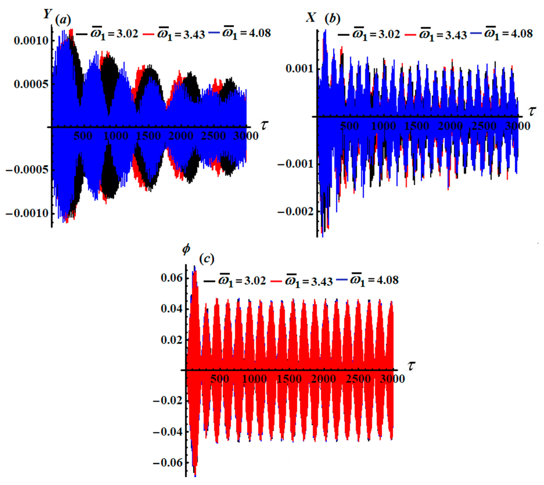
Figure 5, Figure 6 and Figure 7 illustrate the time histories of the attained approximate analytic solutions of $Y,X$, and $\varphi$ till the third order of approximation. These figures were drawn when the previously used data with various values of ${\overline{\omega }}_j(j=1,2,3)$ were used. According to the plotted curves in these figures, we can conclude that these curves have periodic or quasi-periodic forms of wave packets, in which their amplitudes increase (see Figure 5 and Figure 7) and decrease, as shown in Figure 6, with the passage of time until the waves behave in the form of stationary waves at the end of the examined period of time.

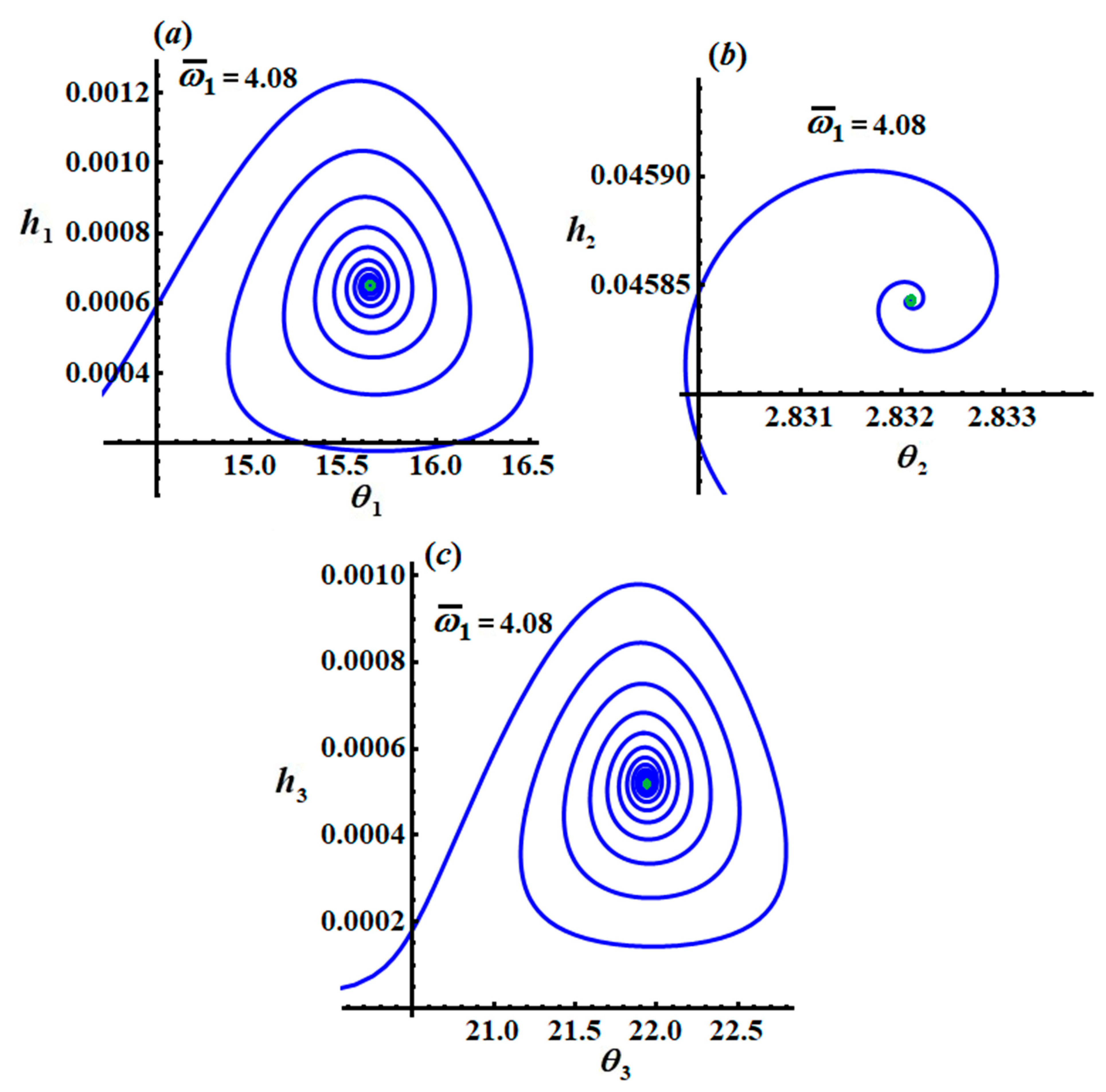
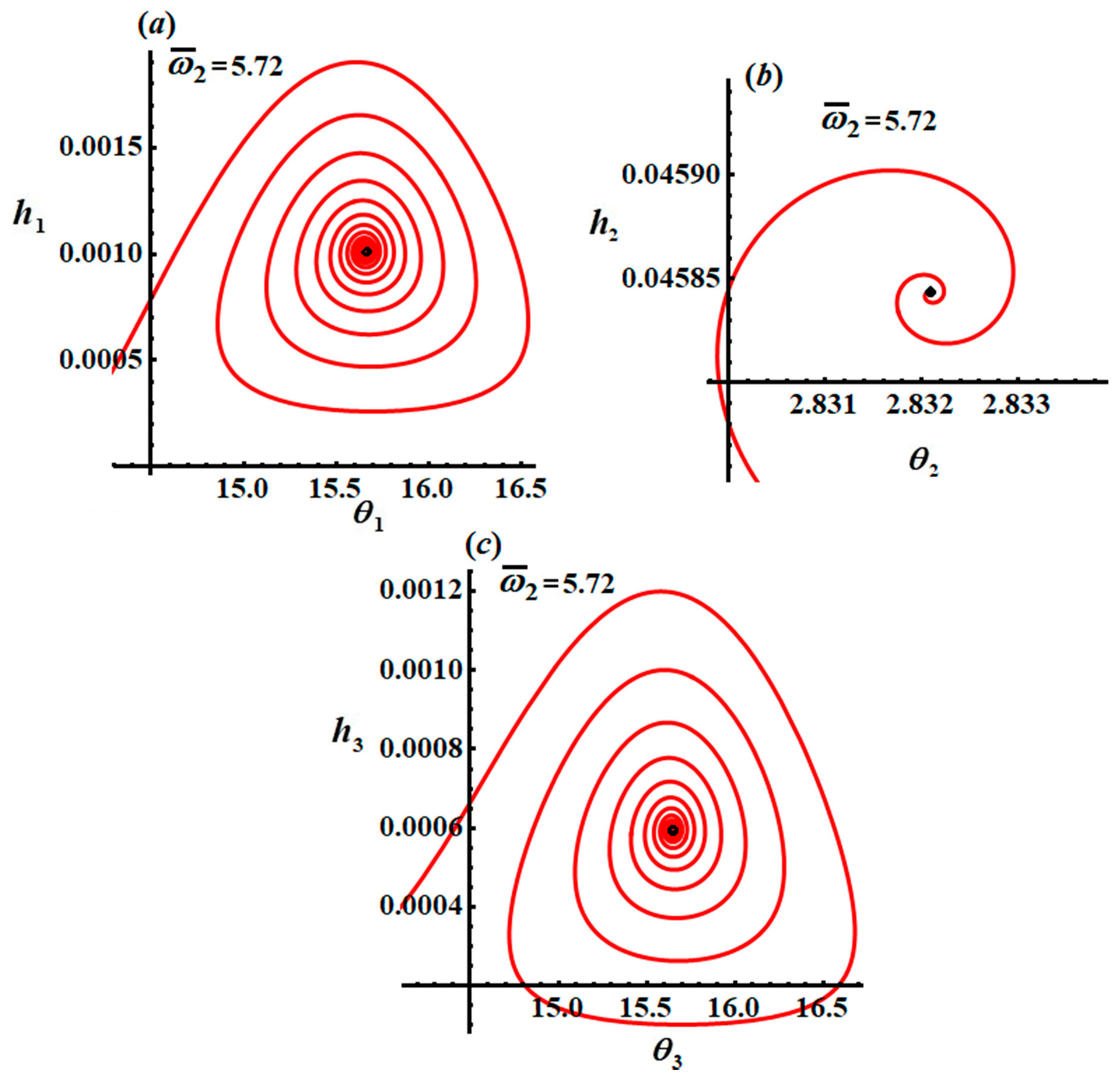
To follow up on the vibrations of the examined system to investigate whether it is stable and to understand the specific transference of motion, the system of Equation (46) permits us to focus on this knowledge. The plotted trajectories of the modified amplitudes and phases are regarded as the best way to depict the system’s behavior.

The track projections on specific space planes are plotted in Figure 8, Figure 9 and Figure 10, when ${\overline{\omega }}_1=4.08,\hspace{0.17em}\hspace{0.17em}{\overline{\omega }}_2=5.72\hspace{0.17em}$, and ${\overline{\omega }}_3=8.37$, respectively. The curves of these figures have spiral forms toward one point, in which the green, black, and red solid points in these figures refer to a stable state. After the transient state, we find that all pathways tend to have steady-state behavior.

4. Solutions in the Steady State

The main objective of this section is to examine the oscillations of the considered system in the steady state. It is known that this case is generated when the transient processes disappear due to the presence of damping [37,38]. Then, we consider the zero value of the left hand side of Equation (46), i.e., $\frac{d{\theta }_j}{dt}=0,\hspace{0.17em}\hspace{0.17em}\frac{d{h}_j}{dt}=0\hspace{0.17em}\hspace{0.17em}\hspace{0.17em}(j=1,\hspace{0.17em}2,\hspace{0.17em}3)$. Therefore, we can easily obtain the following system of six algebraic equations:

$$\begin{array}{l}{h}_1{\sigma }_1+\frac{{\beta }^2{\omega }_1^5{h}_1}{4{({\omega }_1^2-{\omega }_2^2)}^3}[-{\omega }_1^2(4{\omega }_1^2+11)+{\omega }_2^2(7-4{\omega }_2^2)+8{\omega }_1^2{\omega }_2^2]+\frac{f_1}{2{\omega }_1}cos{\theta }_1=0,\\ -\frac{1}{2}{h}_1{c}_1+\frac{f_1}{2{\omega }_1}sin{\theta }_1=0,\\ h_2{\sigma }_2-\frac{6{\omega }_1^2{h}_1^2{h}_2}{8({\omega }_1^2-4){({\omega }_1^2-{\omega }_2^2)}^2}({\omega }_2^2-2{\omega }_1^2+1)+\frac{h_2^3}{16{\omega }_2^2({\omega }_2^2-4)}({\omega }_2^4-25{\omega }_2^2+24)\\ -\frac{6h_3^2{h}_2}{8({\omega }_2^2-4)}({\omega }_2^2-1)+\frac{f_2}{2}cos{\theta }_2=0,\\ -\frac{1}{2}{h}_2{c}_2+\frac{f_2}{2}sin{\theta }_2=0,\\ h_3{\sigma }_3+\frac{{\beta }^2{\omega }_2^5{h}_3}{4{({\omega }_1^2-{\omega }_2^2)}^3}({\omega }_2^2-3{\omega }_1^2)+\frac{h_2^2{h}_3}{8{\omega }_2^2({\omega }_2+2)}[3+2{\omega }_2({\omega }_2+2)]+\frac{f_3}{2{\omega }_2}cos{\theta }_3=0,\\ -\frac{1}{2}{h}_3{c}_3+\frac{f_3}{2{\omega }_2}sin{\theta }_3=0.\end{array}$$

(47)

A closer look into this system shows that if we remove the phases ${\theta }_j\hspace{0.17em}\hspace{0.17em}(j=1,2,3)$, the following non-linear algebraic equations of amplitudes and frequencies are obtained:

$$\begin{array}{l}{f}_1^2=4{\omega }_1^2\{{[h_1{\sigma }_1+\frac{{\beta }^2{\omega }_1^5{h}_1}{4{({\omega }_1^2-{\omega }_2^2)}^3}(-{\omega }_1^2(4{\omega }_1^2+11)+{\omega }_2^2(7-4{\omega }_2^2)+8{\omega }_1^2{\omega }_2^2)]}^2+\frac{1}{4}{h}_1^2{c}_1^2\},\\ f_2^2=4\{[h_2{\sigma }_2-\frac{6{\omega }_1^2{h}_1^2{h}_2}{8({\omega }_1^2-4){({\omega }_1^2-{\omega }_2^2)}^2}({\omega }_2^2-2{\omega }_1^2+1)+\frac{h_2^3}{16{\omega }_2^2({\omega }_2^2-4)}({\omega }_2^4-25{\omega }_2^2+24)\\ -\frac{6h_3^2{h}_2}{8({\omega }_2^2-4)}({\omega }_2^2-1){]}^2+\frac{1}{4}{h}_2^2{c}_2^2\},\\ f_3^2=4{\omega }_2^2\{[h_3{\sigma }_3+\frac{{\beta }^2{\omega }_2^5{h}_3}{4{({\omega }_1^2-{\omega }_2^2)}^3}({\omega }_2^2-3{\omega }_1^2)+\frac{h_2^2{h}_3}{8{\omega }_2^2({\omega }_2+2)}\\ \times (3+2{\omega }_2({\omega }_2+2)){]}^2+\frac{1}{4}{h}_3^2{c}_3^2\}.\end{array}$$

(48)

For further investigation of the stability, we will examine the behavior of the dynamical system in a region close to the fixed points. To complete this task, we will consider the following forms of amplitudes and phases:

$$\begin{array}{ccc}{h}_1=h_{10}+h_{11},& \hspace{0.17em}\hspace{0.17em}{h}_2=h_{20}+h_{21},& \hspace{0.17em}\hspace{0.17em}{h}_3=h_{30}+h_{31},\\ {\theta }_1={\theta }_{10}+{\theta }_{11},& \hspace{0.17em}\hspace{0.17em}{\theta }_2={\theta }_{20}+{\theta }_{21},& \hspace{0.17em}\hspace{0.17em}{\theta }_3={\theta }_{30}+{\theta }_{31},\end{array}$$

(49)

where $h_{10}, h_{20}, h_{30}, {\theta }_{10}, {\theta }_{20}$, and ${\theta }_{30}$ are the solutions in the steady state, while $h_{11}, h_{21}, h_{31}, {\theta }_{11}, {\theta }_{21}$, and ${\theta }_{31}$ are the corresponding perturbations, which are assumed to be very small.

The substitution of Equation (49) into Equation (46) yields the following equations:

$$\begin{array}{l}{h}_{10}\frac{d{\theta }_{11}}{d\tau }=h_{11}{\sigma }_1-\frac{f_1}{2{\omega }_1}{\theta }_{11}\sin {\theta }_{10}+\hspace{0.17em}{G}_1,\\ \frac{d{h}_{11}}{d\tau }=-\frac{1}{2}{h}_{11}{c}_1+\frac{f_1}{2{\omega }_1}{\theta }_{11}\cos {\theta }_{10},\\ h_{20}\frac{d{\theta }_{21}}{d\tau }=h_{21}{\sigma }_2-\frac{f_2}{2}{\theta }_{21}\sin {\theta }_{20}+G_2,\hspace{0.17em}\hspace{0.17em}\hspace{0.17em}\hspace{0.17em}\hspace{0.17em}\hspace{0.17em}\hspace{0.17em}\hspace{0.17em}\hspace{0.17em}\hspace{0.17em}\hspace{0.17em}\hspace{0.17em}\\ \frac{d{h}_{21}}{d\tau }=-\frac{1}{2}{h}_{21}{c}_2+\frac{f_2}{2}{\theta }_{21}\cos {\theta }_{20},\\ h_{30}\frac{d{\theta }_{31}}{d\tau }=h_{31}{\sigma }_3-\frac{f_3}{2{\omega }_2}{\theta }_{31}\sin {\theta }_{30}+G_3,\\ \frac{d{h}_{31}}{d\tau }=-\frac{1}{2}{h}_{31}{c}_3+\frac{f_3}{2{\omega }_2}{\theta }_{31}\cos {\theta }_{30},\end{array}$$

(50)

where:

$$\begin{array}{l}{G}_1=\frac{{\beta }^2{\omega }_1^5{h}_{11}}{4{({\omega }_1^2-{\omega }_2^2)}^3}[-{\omega }_1^2(4{\omega }_1^2+11)+{\omega }_2^2(7-4{\omega }_2^2)+8{\omega }_1^2{\omega }_2^2],\\ G_2=-\frac{6({\omega }_2^2-1)}{8({\omega }_2^2-4)}(2h_{20}{h}_{30}{h}_{31}+h_{30}^2{h}_{21})\frac{3h_{20}^2{h}_{21}}{16{\omega }_2^2({\omega }_2^2-4)}({\omega }_2^4-25{\omega }_2^2+24)\\ -\frac{6{\omega }_1^2({\omega }_2^2-2{\omega }_1^2+1)}{8({\omega }_1^2-4){({\omega }_1^2-{\omega }_2^2)}^2}(2h_{20}{h}_{10}{h}_{11}+h_{10}^2{h}_{21}),\\ G_3=\frac{[3+2{\omega }_2({\omega }_2+2)]}{8{\omega }_2^2({\omega }_2+2)}(2h_{30}{h}_{20}{h}_{21}+h_{20}^2{h}_{31})+\frac{{\beta }^2{\omega }_2^5{h}_{31}}{4{({\omega }_1^2-{\omega }_2^2)}^3}({\omega }_2^2-3{\omega }_1^2).\end{array}$$

Based on the minuteness of the perturbation functions $h_{11}, h_{21}, h_{31}, {\theta }_{11}, {\theta }_{21}$, and ${\theta }_{31}$, we can express each solution in the form of a linear combination of $S_k\hspace{0.17em}{e}^{\lambda \tau } (k=1,2,\dots ,6)$, where $S_k$ and $\lambda$ are constants and the eigenvalue of the unknown perturbation, respectively.

If the solutions in the steady state (fixed points) $h_{10}, h_{20}, h_{30}, {\theta }_{10}, {\theta }_{20}$, and ${\theta }_{31}$ are stable asymptotically, then the real parts of the roots of the following characteristic equation must be negative:

$${\lambda }^6+{\mathrm{\Gamma }}_1{\lambda }^5+{\mathrm{\Gamma }}_2{\lambda }^4+{\mathrm{\Gamma }}_3{\lambda }^3+{\mathrm{\Gamma }}_4{\lambda }^2+{\mathrm{\Gamma }}_5\lambda +{\mathrm{\Gamma }}_6=0\hspace{0.17em},$$

(51)

where ${\mathrm{\Gamma }}_k$ are functions depending on the parameters $h_{10}, h_{20}, h_{30}, {\theta }_{10}, {\theta }_{20}, {\theta }_{30}, f_1, f_2$, and $f_3$ (see Appendix B).

Referring to the above, the substantial conditions for the stability of the solutions in the steady state can be written according to the criterion of Routh–Hurwitz [32] in the following forms:

$$\begin{array}{l}{\mathrm{\Gamma }}_1>0, {\mathrm{\Gamma }}_1{\mathrm{\Gamma }}_2-{\mathrm{\Gamma }}_3>0,\\ {\mathrm{\Gamma }}_3({\mathrm{\Gamma }}_1{\mathrm{\Gamma }}_2-{\mathrm{\Gamma }}_3)+{\mathrm{\Gamma }}_1({\mathrm{\Gamma }}_5-{\mathrm{\Gamma }}_1{\mathrm{\Gamma }}_4)>0,\\ {\mathrm{\Gamma }}_1({\mathrm{\Gamma }}_2{\mathrm{\Gamma }}_3{\mathrm{\Gamma }}_4-{{\mathrm{\Gamma }}_2}^2{\mathrm{\Gamma }}_5+2{\mathrm{\Gamma }}_4{\mathrm{\Gamma }}_5-{\mathrm{\Gamma }}_3{\mathrm{\Gamma }}_6)+{\mathrm{\Gamma }}_3({\mathrm{\Gamma }}_2{\mathrm{\Gamma }}_5-{\mathrm{\Gamma }}_3{\mathrm{\Gamma }}_4)+{{\mathrm{\Gamma }}_1}^2({\mathrm{\Gamma }}_2{\mathrm{\Gamma }}_6-{{\mathrm{\Gamma }}_4}^2)-{{\mathrm{\Gamma }}_5}^2>0,\\ -{\mathrm{\Gamma }}_5({\mathrm{\Gamma }}_4(-{\mathrm{\Gamma }}_1{\mathrm{\Gamma }}_2{\mathrm{\Gamma }}_3+{{\mathrm{\Gamma }}_3}^2+{{\mathrm{\Gamma }}_1}^2{\mathrm{\Gamma }}_4)+{\mathrm{\Gamma }}_1({{\mathrm{\Gamma }}_2}^2-2{\mathrm{\Gamma }}_4){\mathrm{\Gamma }}_5-{\mathrm{\Gamma }}_2{\mathrm{\Gamma }}_3{\mathrm{\Gamma }}_5+{{\mathrm{\Gamma }}_5}^2)\\ +({{\mathrm{\Gamma }}_3}^3-{\mathrm{\Gamma }}_1{\mathrm{\Gamma }}_3({\mathrm{\Gamma }}_2{\mathrm{\Gamma }}_3+3{\mathrm{\Gamma }}_5)+{{\mathrm{\Gamma }}_1}^2({\mathrm{\Gamma }}_3{\mathrm{\Gamma }}_4+2{\mathrm{\Gamma }}_2{\mathrm{\Gamma }}_5)){\mathrm{\Gamma }}_6-{{\mathrm{\Gamma }}_1}^3{{\mathrm{\Gamma }}_6}^2>0,\\ {\mathrm{\Gamma }}_6(-{\mathrm{\Gamma }}_5({\mathrm{\Gamma }}_4(-{\mathrm{\Gamma }}_1{\mathrm{\Gamma }}_2{\mathrm{\Gamma }}_3+{{\mathrm{\Gamma }}_3}^2+{{\mathrm{\Gamma }}_1}^2{\mathrm{\Gamma }}_4)+{\mathrm{\Gamma }}_1({{\mathrm{\Gamma }}_2}^2-2{\mathrm{\Gamma }}_4){\mathrm{\Gamma }}_5-{\mathrm{\Gamma }}_2{\mathrm{\Gamma }}_3{\mathrm{\Gamma }}_5+{{\mathrm{\Gamma }}_5}^2)\\ +({{\mathrm{\Gamma }}_3}^3-{\mathrm{\Gamma }}_1{\mathrm{\Gamma }}_3({\mathrm{\Gamma }}_2{\mathrm{\Gamma }}_3+3{\mathrm{\Gamma }}_5)+{{\mathrm{\Gamma }}_1}^2({\mathrm{\Gamma }}_3{\mathrm{\Gamma }}_4+2{\mathrm{\Gamma }}_2{\mathrm{\Gamma }}_5)){\mathrm{\Gamma }}_6-{{\mathrm{\Gamma }}_1}^3{{\mathrm{\Gamma }}_6}^2)>0.\end{array}$$

(52)

5. Non-Linear Analysis of Stability

The main aim of this section is to investigate the stability analysis of the considered system using the non-linear stability approach of Routh–Hurwitz. The examined system is exposed to various forces and moments, such as the excited harmonic forces $F_1,F_3$ and the moment $M_{\varphi }$. It is found that the natural frequencies $\overline{{\omega }_j}\hspace{0.17em}(j=1,2,3),$ damping coefficients $c_j$, and the parameters of detuning perform a crucial destabilizing role in the criteria’s stability. To plot the stability diagrams of the system of Equation (46), the previous values of the different parameters are used. The modified amplitudes $h_{j\hspace{0.17em}\hspace{0.17em}}(j=1,2,3)$ are shown with the detuning parameter ${\sigma }_1$ in Figure 11, Figure 12, Figure 13 and Figure 14 for different values of $\overline{{\omega }_j}$ when ${\sigma }_2={\sigma }_3=0$. 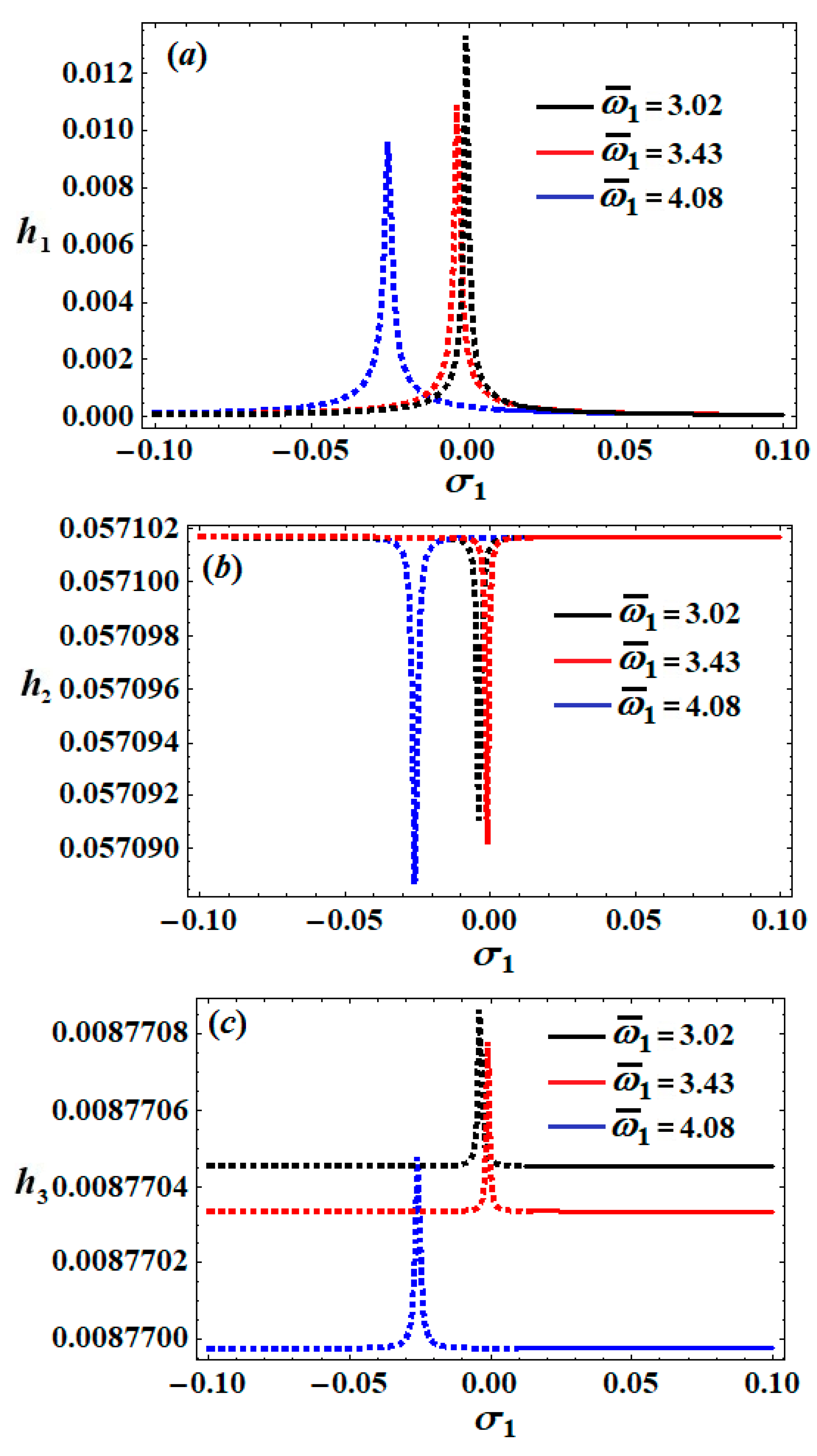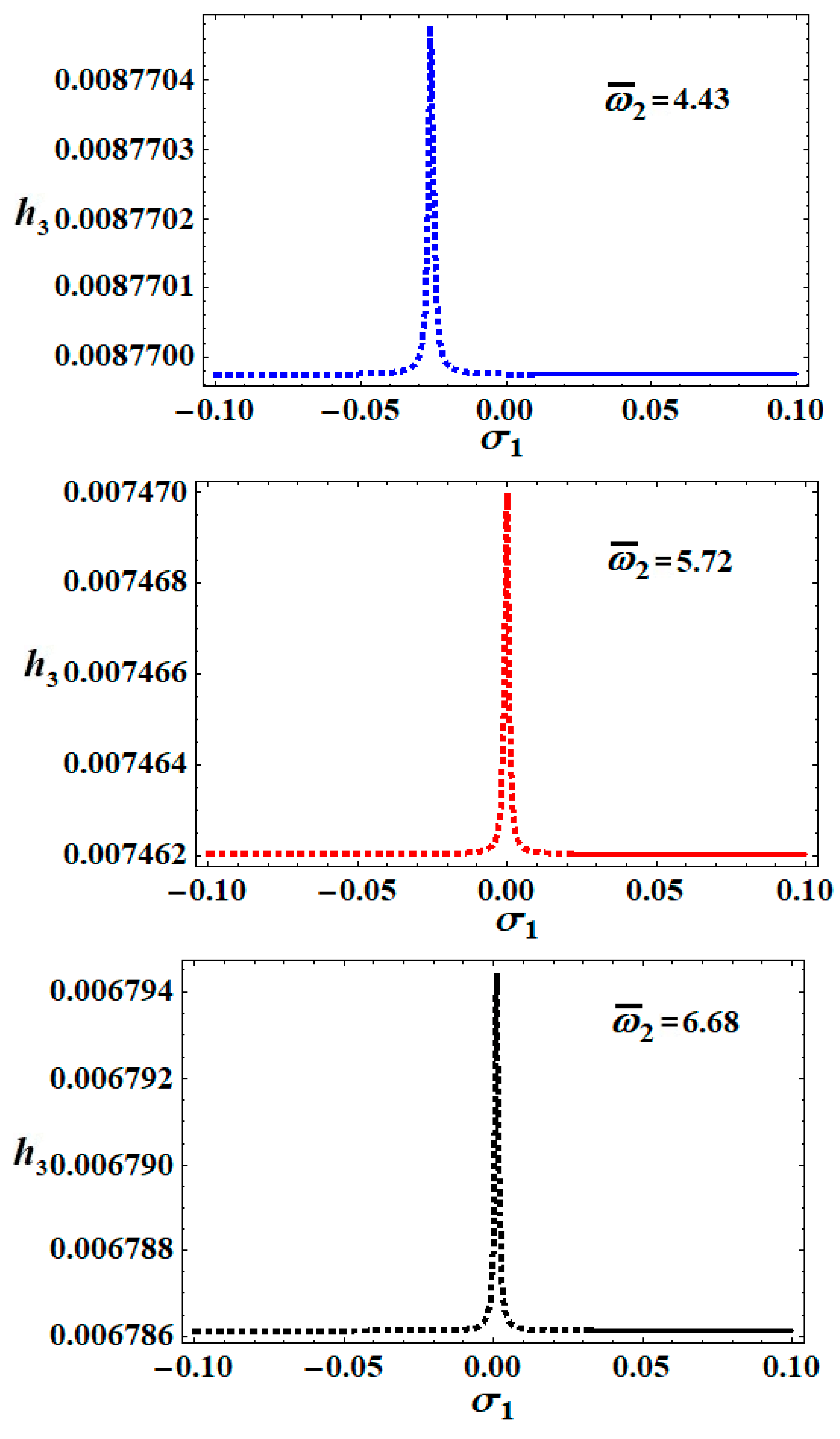The outlined curves of these figures contain the possible fixed points. Resonance curves are plotted in Figure 11, Figure 12, Figure 13 and Figure 14 according to the previous data of parameters.

Each of the resonance curves has different stable and unstable regions with the various values of the natural frequencies ${\overline{\omega }}_1$ and ${\overline{\omega }}_2$ (see Figure 11, Figure 12, Figure 13 and Figure 14). More precisely, the inspection of parts of Figure 11 shows that the instability and stability ranges are $-0.1<{\sigma }_1<0.009$ and $0.009\le {\sigma }_1<0.1$, respectively, as indicated in Figure 11 in blue. On the other hand, when ${\overline{\omega }}_1=3.43$, the red curves represent the instability and stability ranges of $-0.1<{\sigma }_1<0.012$ and $0.012\le {\sigma }_1<0.1$, respectively, while the black curves represent the areas of instability and stability when ${\overline{\omega }}_1=3.02$, which are $-0.1<{\sigma }_1<0.014$ and $0.014\le {\sigma }_1<0.1$, respectively. The included curves of each part have different fixed points associated with the different values of ${\overline{\omega }}_1$, as indicated in Figure 11. Moreover, the instability regions decrease with an increase in the value of ${\overline{\omega }}_1$, due to the impact of the natural frequency ${\overline{\omega }}_1$.

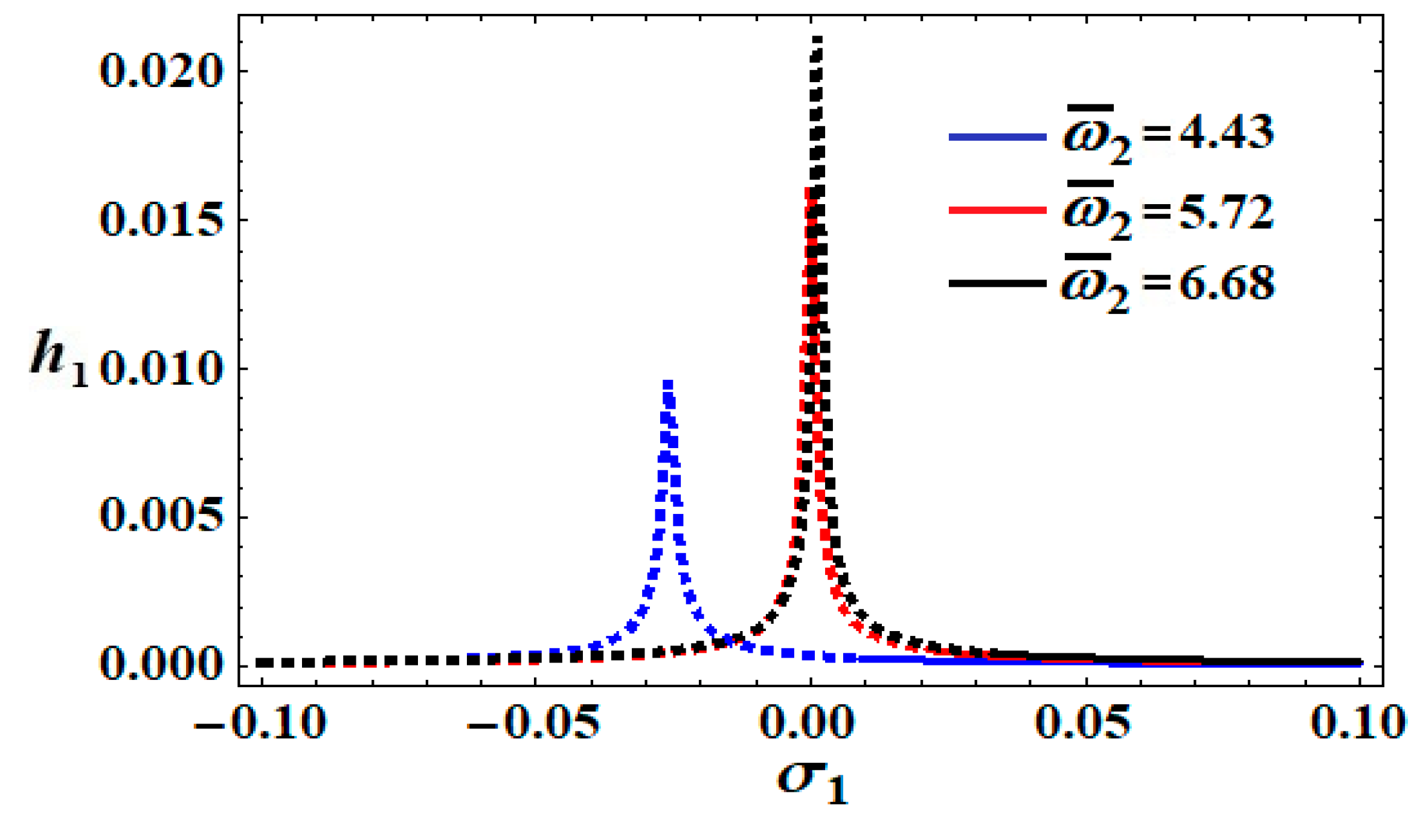
Figure 12 illustrates the different ranges of stability criterion, where the instability and stability areas, indicated in blue, are determined according to the ranges $-0.1<{\sigma }_1<0.009$ and $0.009\le {\sigma }_1<0.1$, respectively. At ${\overline{\omega }}_2=5.72$, the red curves show the instability and stability areas with ranges $-0.1<{\sigma }_1<0.021$ and $0.021\le {\sigma }_1<0.1$, respectively, while the black curves show the instability and stability areas at ${\overline{\omega }}_2=6.68$, which are $-0.1<{\sigma }_1<0.033$ and $0.033\le {\sigma }_1<0.1$, respectively.

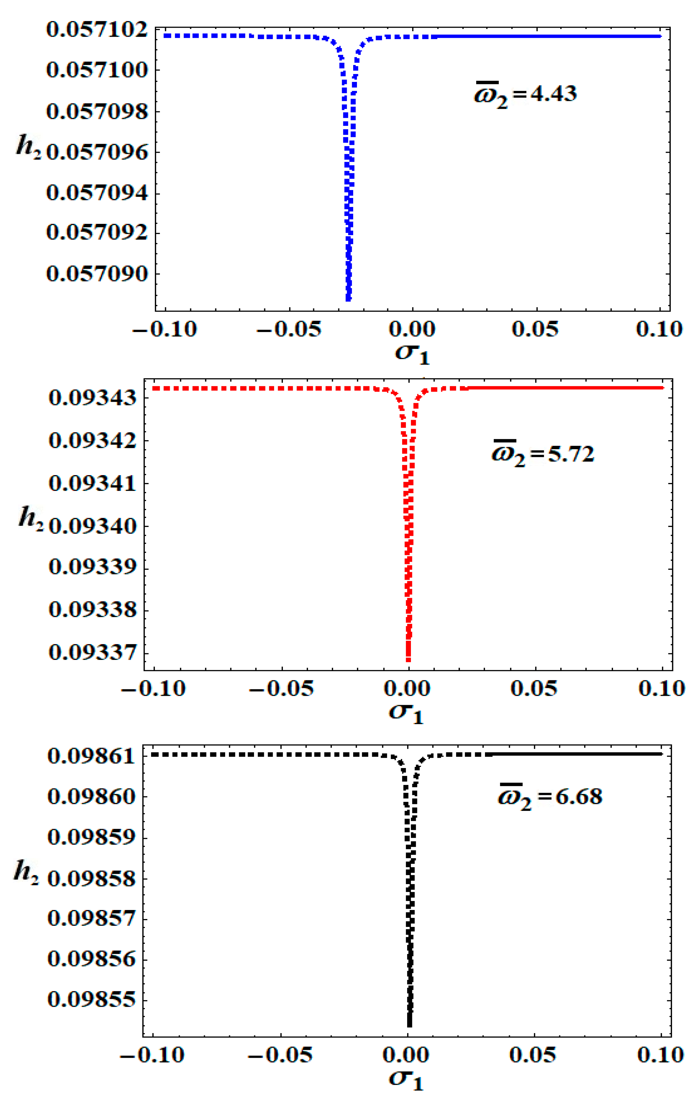
According to the calculations of the graphed curves in Figure 13 and Figure 14, we can state that three different peak fixed points are produced when ${\overline{\omega }}_2$ has different values for the resonance curves of $h_2$ and $h_3$, which are varied with ${\sigma }_1$. The instability and the stability areas become $-0.1<{\sigma }_1<0.009$ and $0.009\le {\sigma }_1<0.1$, respectively, denoted in blue (see Figure 13 and Figure 14), while at ${\overline{\omega }}_2=5.72$, the red curves indicate the instability and stability areas $-0.1<{\sigma }_1<0.021$ and $0.021\le {\sigma }_1<0.1$, respectively. On the other hand, the black curves represent the areas of instability and stability when ${\overline{\omega }}_2=6.68$, which are $-0.1<{\sigma }_1<0.033$ and $0.033\le {\sigma }_1<0.1$, respectively.

To clarify the properties of the non-linear amplitudes of the system of Equations (46) and to examine their stabilities, we consider the following transformations [39]:

$$A_j=[U_j({\tau }_1,{\tau }_2)+i{V}_j({\tau }_1,{\tau }_2)]\hspace{0.17em}{e}^{i{\tilde{\sigma }}_j{\tau }_1};\hspace{0.17em}\hspace{0.17em}\hspace{0.17em}\hspace{0.17em}\hspace{0.17em}(j=1,2,3)$$

(53)

where:

$$U_j=\epsilon \hspace{0.17em}{u}_j,\hspace{0.17em}\hspace{0.17em}\hspace{0.17em}\hspace{0.17em}\hspace{0.17em}\hspace{0.17em}\hspace{0.17em}\hspace{0.17em}{V}_j=\epsilon \hspace{0.17em}{v}_j.$$

Substituting the operators (13) and the previous transformation (53) into the system of the ODE (46), we can equate the real parts and the imaginary parts with zero to obtain of the following system:

$$\begin{array}{l}\frac{d{u}_1}{d\tau }=v_1\{{\sigma }_1+G_4[-{\omega }_1^2(4{\omega }_1^2+11)+{\omega }_2^2(7-4{\omega }_2^2)+8{\omega }_1^2{\omega }_2^2]\}-\frac{c_1}{2}{u}_1,\\ \frac{d{v}_1}{d\tau }=u_1\{{\sigma }_1+G_4[-{\omega }_1^2(4{\omega }_1^2+11)+{\omega }_2^2(7-4{\omega }_2^2)+8{\omega }_1^2{\omega }_2^2]\}+\frac{c_1}{2}{v}_1-\frac{f_1}{4{\omega }_1},\\ \frac{d{u}_2}{d\tau }=v_2[{\sigma }_2-G_5(u_1^2+v_1^2)+G_6(u_2^2+v_2^2)+G_7(u_3^2+v_3^2)]-\frac{c_2}{2}{u}_2,\\ \frac{d{v}_2}{d\tau }=u_2[{\sigma }_2+G_5(u_1^2+v_1^2)-G_6(u_2^2+v_2^2)-G_7(u_3^2+v_3^2)]-\frac{c_2}{2}{v}_2-\frac{f_2}{4},\\ \frac{d{u}_3}{d\tau }=v_3[{\sigma }_3+G_8+G_9(u_2^2+v_2^2)]-\frac{c_3}{2}{u}_3,\\ \frac{d{v}_3}{d\tau }=u_3[{\sigma }_3-G_8-G_9(u_2^2+v_2^2)]-\frac{c_3}{2}{v}_3-\frac{f_3}{4{\omega }_2},\end{array}$$

(54)

where:

$$\begin{array}{l}{G}_4=\frac{{\beta }^2{\omega }_1^5}{4{({\omega }_1^2-{\omega }_2^2)}^3},\hspace{0.17em}\hspace{0.17em}\hspace{0.17em}\hspace{0.17em}\hspace{0.17em}\hspace{0.17em}\hspace{0.17em}\hspace{0.17em}{G}_5=\frac{3{\omega }_1^4{({\omega }_2^2-2{\omega }_1^2+1)}^2}{({\omega }_1^2-4){({\omega }_1^2-{\omega }_2^2)}^2},\hspace{0.17em}\hspace{0.17em}\hspace{0.17em}\hspace{0.17em}\hspace{0.17em}\hspace{0.17em}\hspace{0.17em}\hspace{0.17em}{G}_6=\frac{({\omega }_2^4-25{\omega }_2^2+24)}{4{\omega }_2^2({\omega }_2^2-4)},\\ G_7=\frac{3({\omega }_2^2-1)}{8({\omega }_2^2-4)},\hspace{0.17em}\hspace{0.17em}\hspace{0.17em}\hspace{0.17em}\hspace{0.17em}\hspace{0.17em}\hspace{0.17em}\hspace{0.17em}{G}_8=\frac{{\beta }^2\hspace{0.17em}{\omega }_2^5}{4{({\omega }_1^2-{\omega }_2^2)}^3},\hspace{0.17em}\hspace{0.17em}\hspace{0.17em}\hspace{0.17em}\hspace{0.17em}\hspace{0.17em}\hspace{0.17em}\hspace{0.17em}{G}_9=\frac{[3+2{\omega }_2({\omega }_2+2)]}{8{\omega }_2^2({\omega }_2+2)}.\end{array}$$

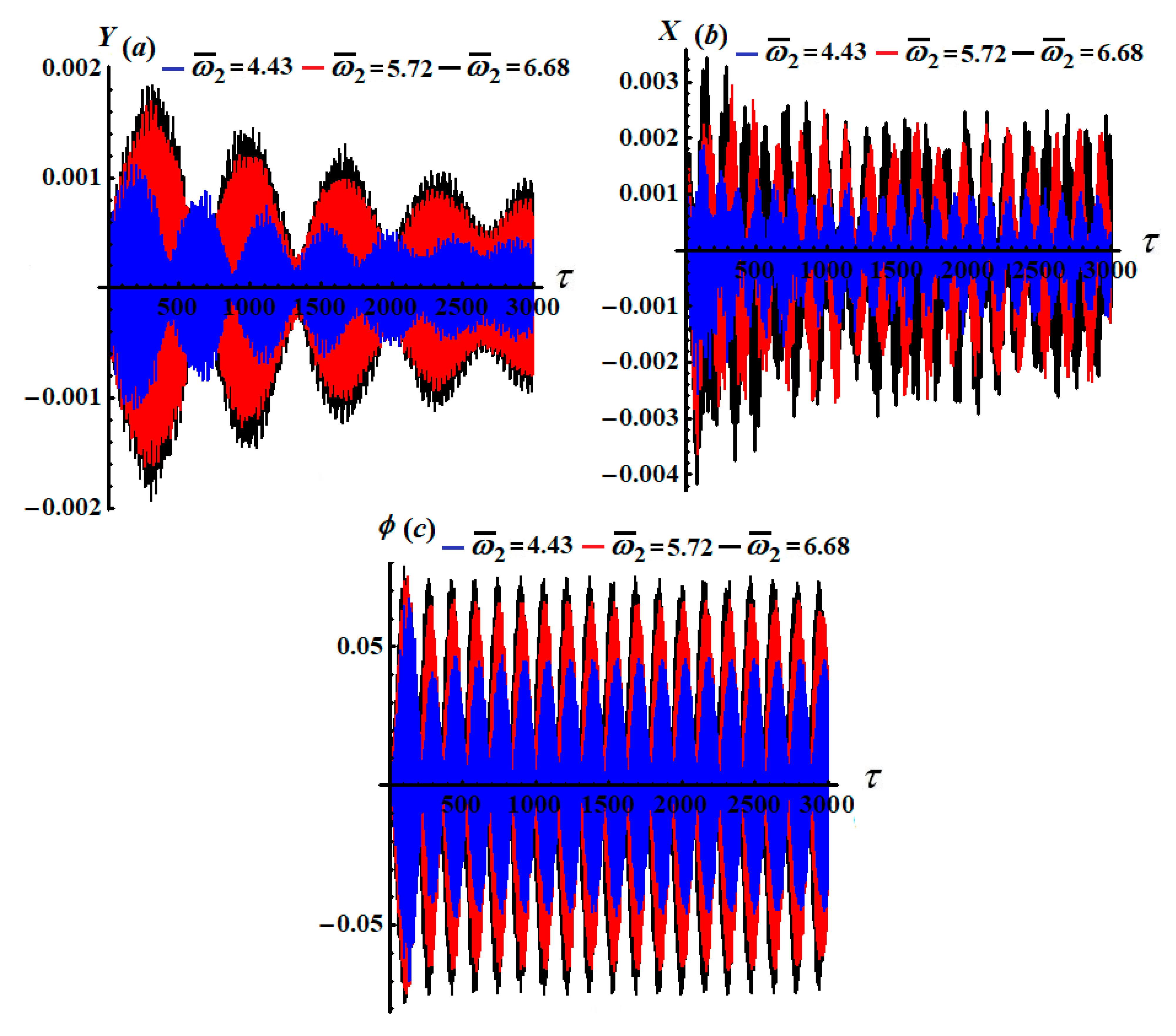
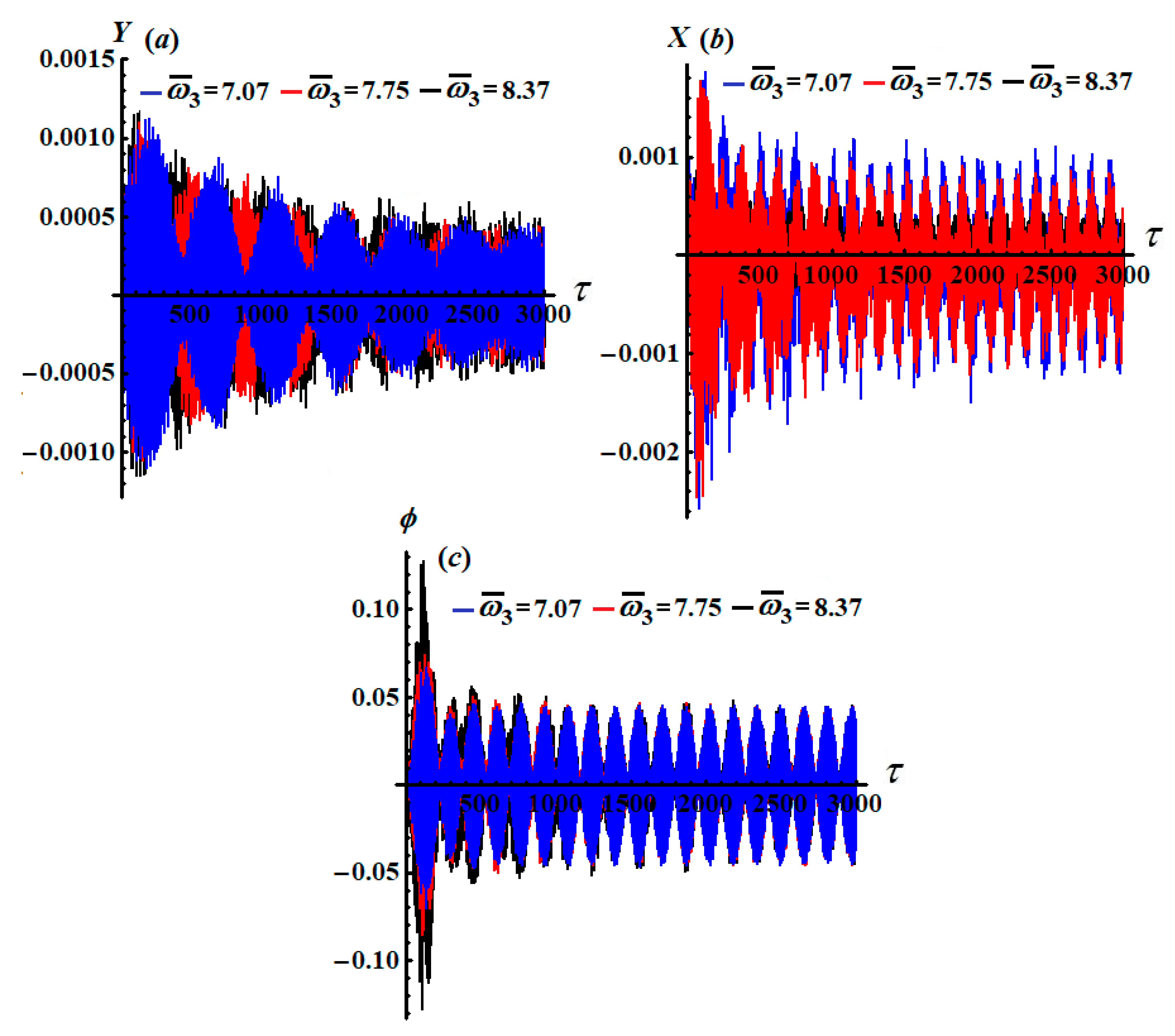
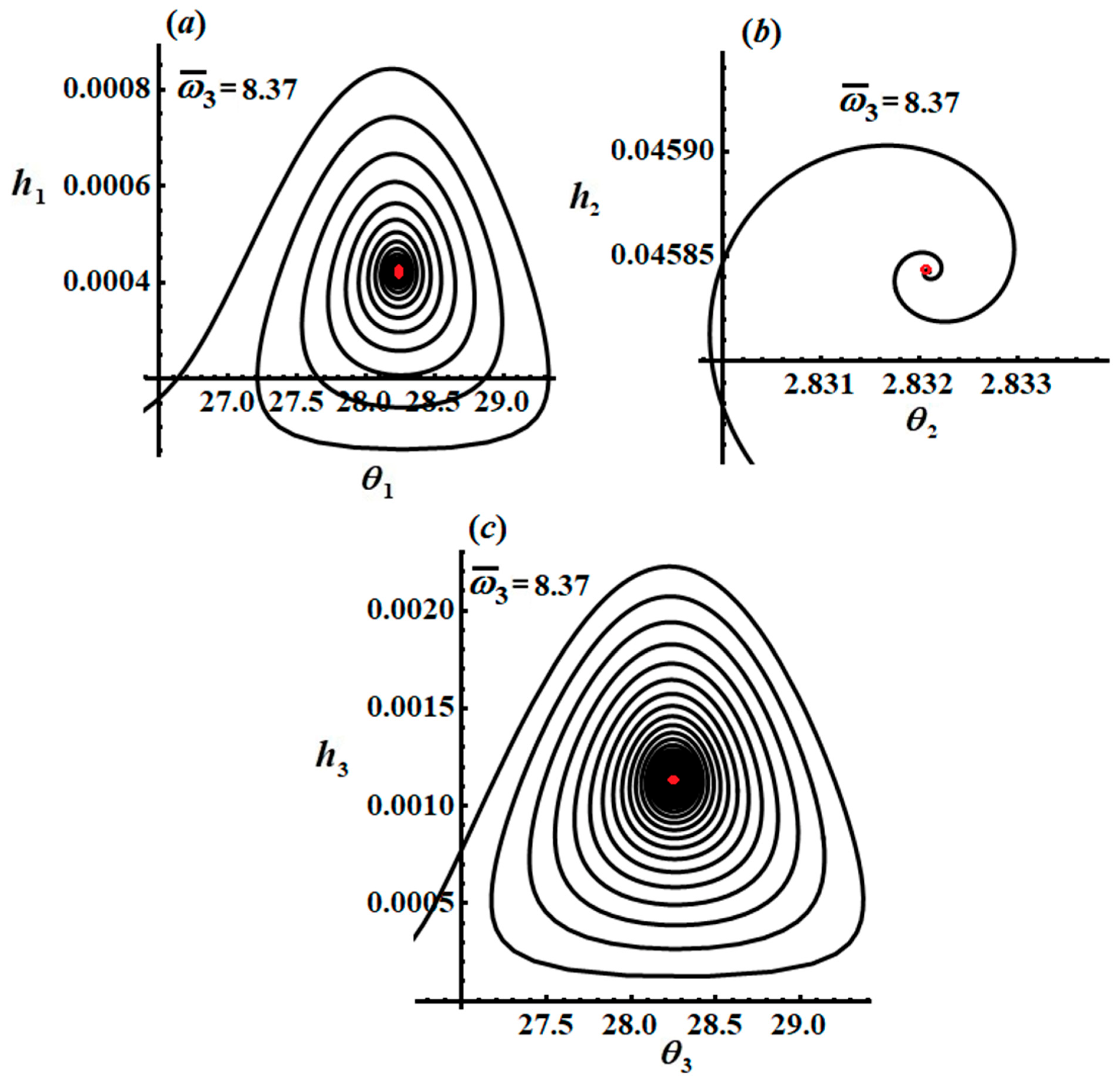
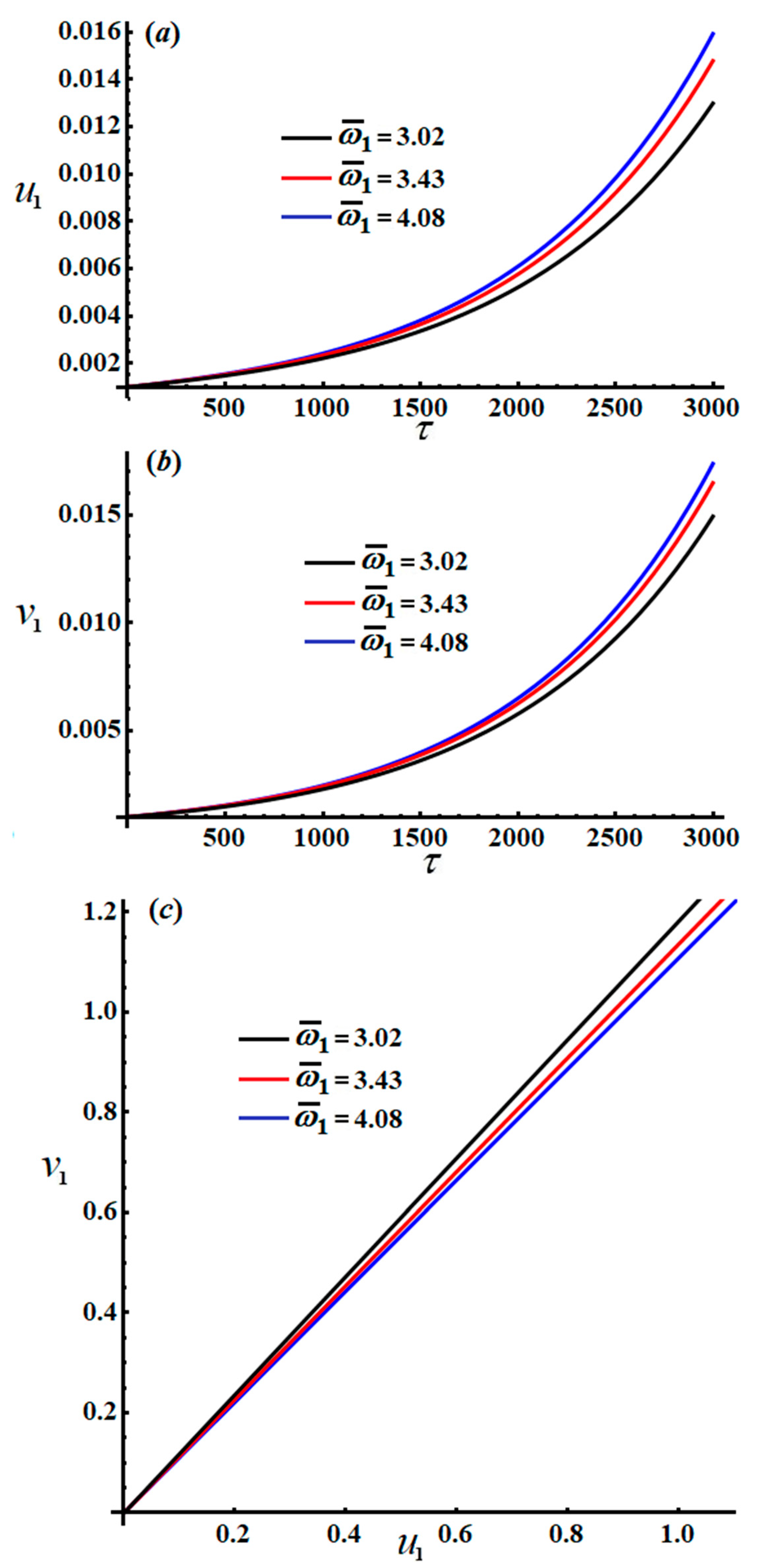
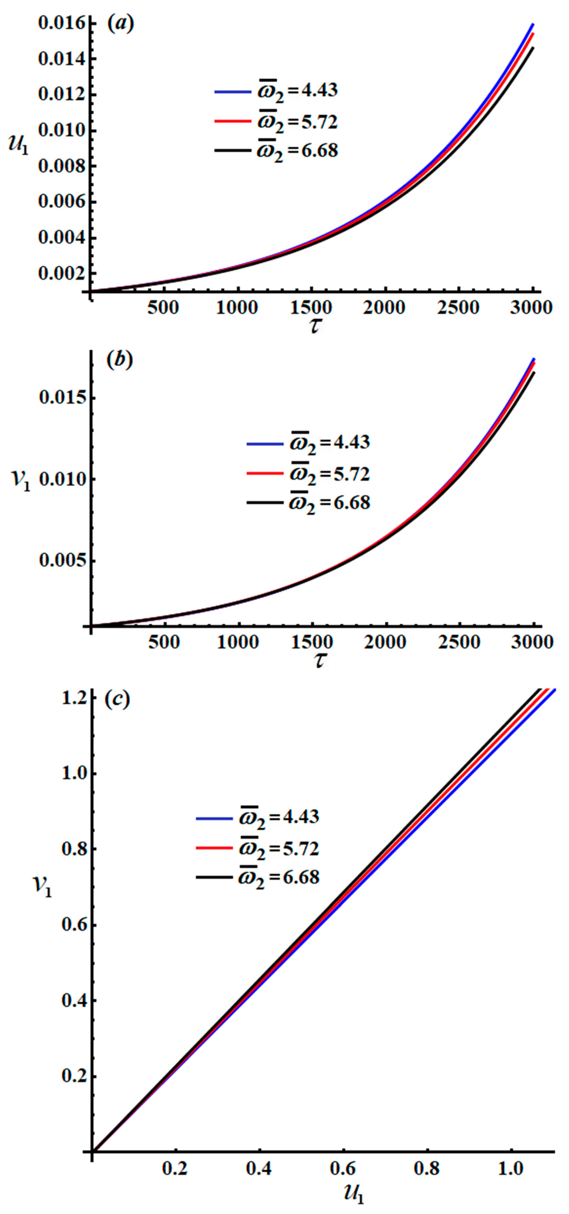
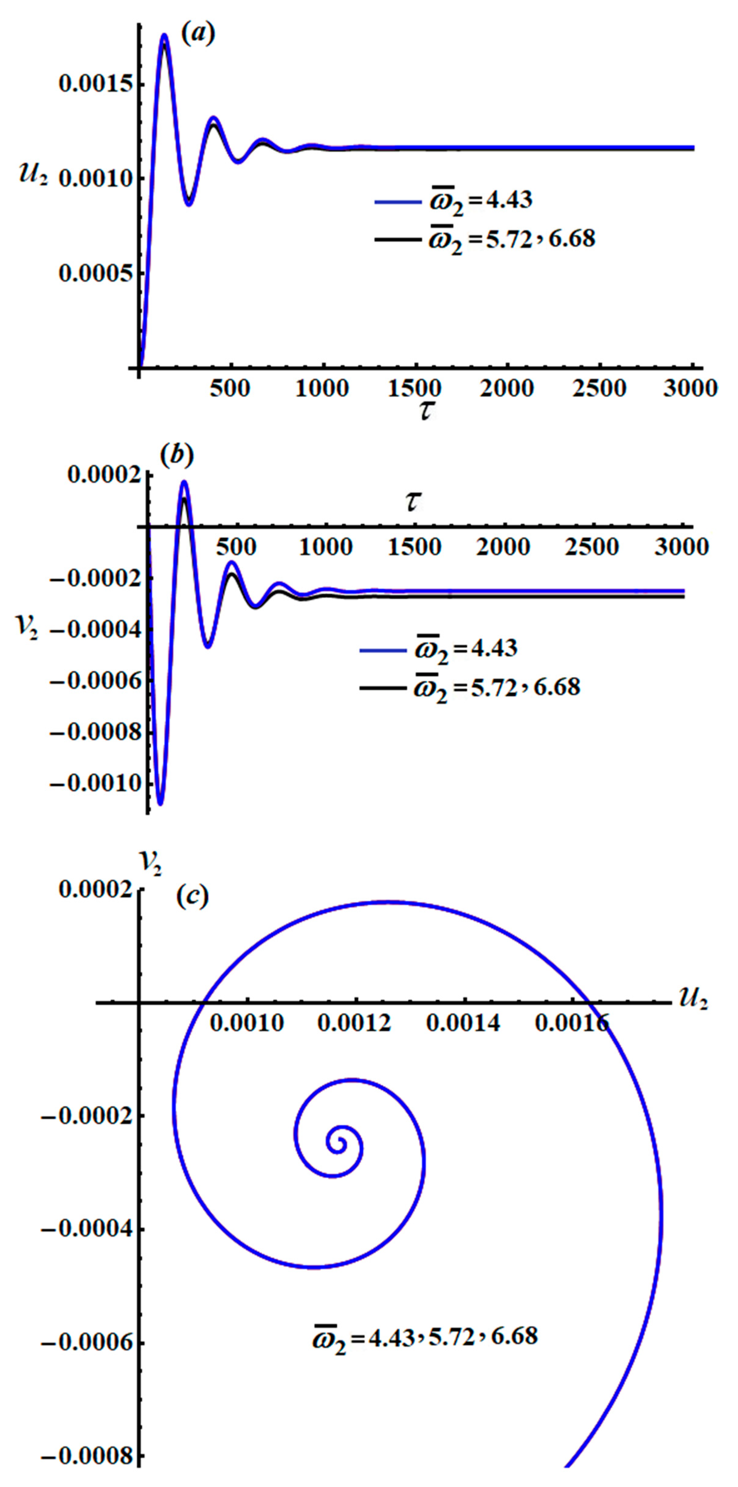
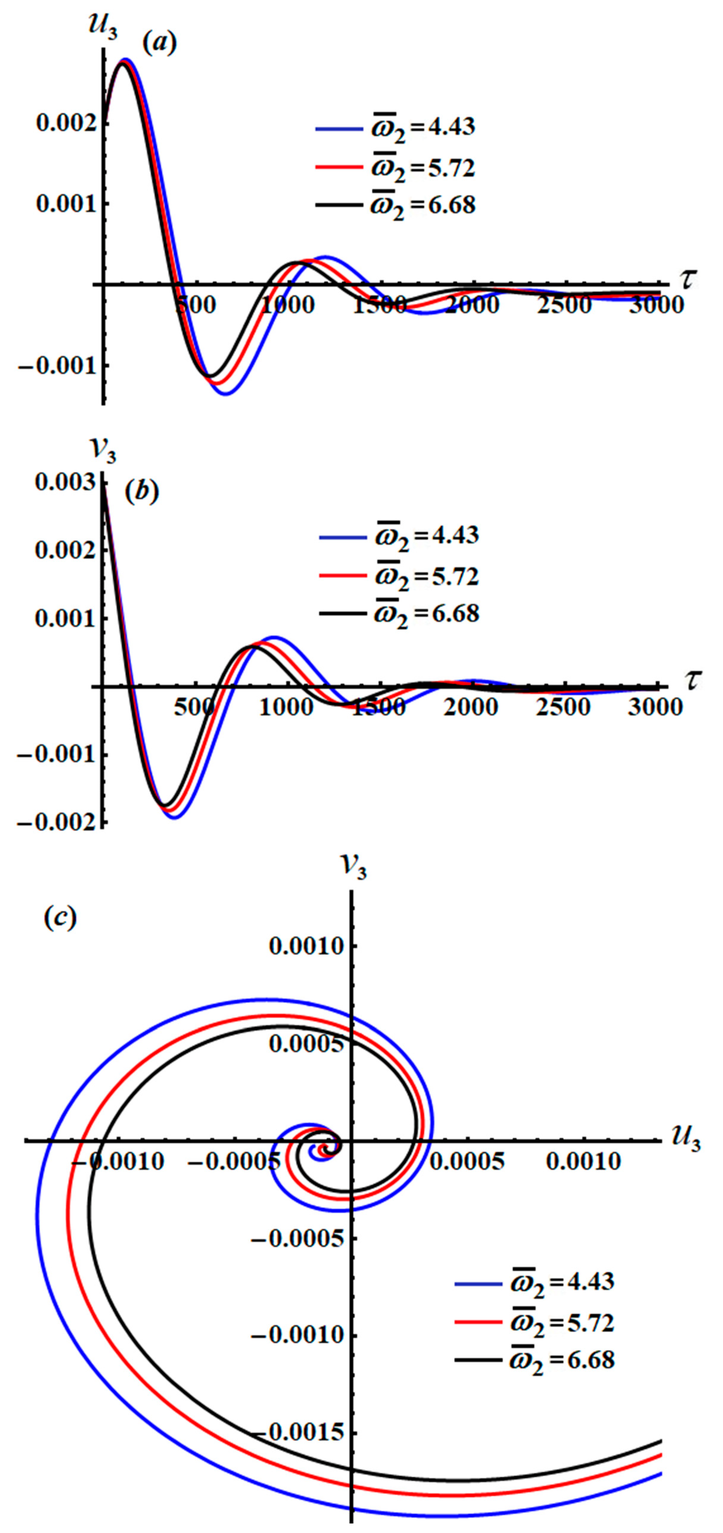
The modified amplitudes can be subsequently rationalized through the time in various parametric regions; the properties of the amplitudes are presented in phase plane curves shown in Figure 15, Figure 16, Figure 17, Figure 18, Figure 19 and Figure 20, taking into account the data from previously used parameters.

Parts of Figure 15, Figure 16, Figure 17, Figure 18, Figure 19 and Figure 20 explore the changing of the new justified phases $u_j$ and $v_j\hspace{0.17em}\hspace{0.17em}\hspace{0.17em}(j=1,2,3)$, as stated in the system of Equation (54), via $\tau$ as shown in parts (a) and (b). The projections of the modulation equation trajectories on the phase planes $u_j{v}_j$ are graphed in part (c) of these figures. The indicated curves of Figure 15, Figure 16, Figure 17, Figure 18, Figure 19 and Figure 20 are calculated when ${\overline{\omega }}_1=(3.02,3.43,4.08)$ and ${\overline{\omega }}_2=(4.43,5.72,6.68)$, respectively, besides the values of the detuning parameters ${\sigma }_1=0.01,$ ${\sigma }_2=0.02$, and ${\sigma }_3=0.03$.

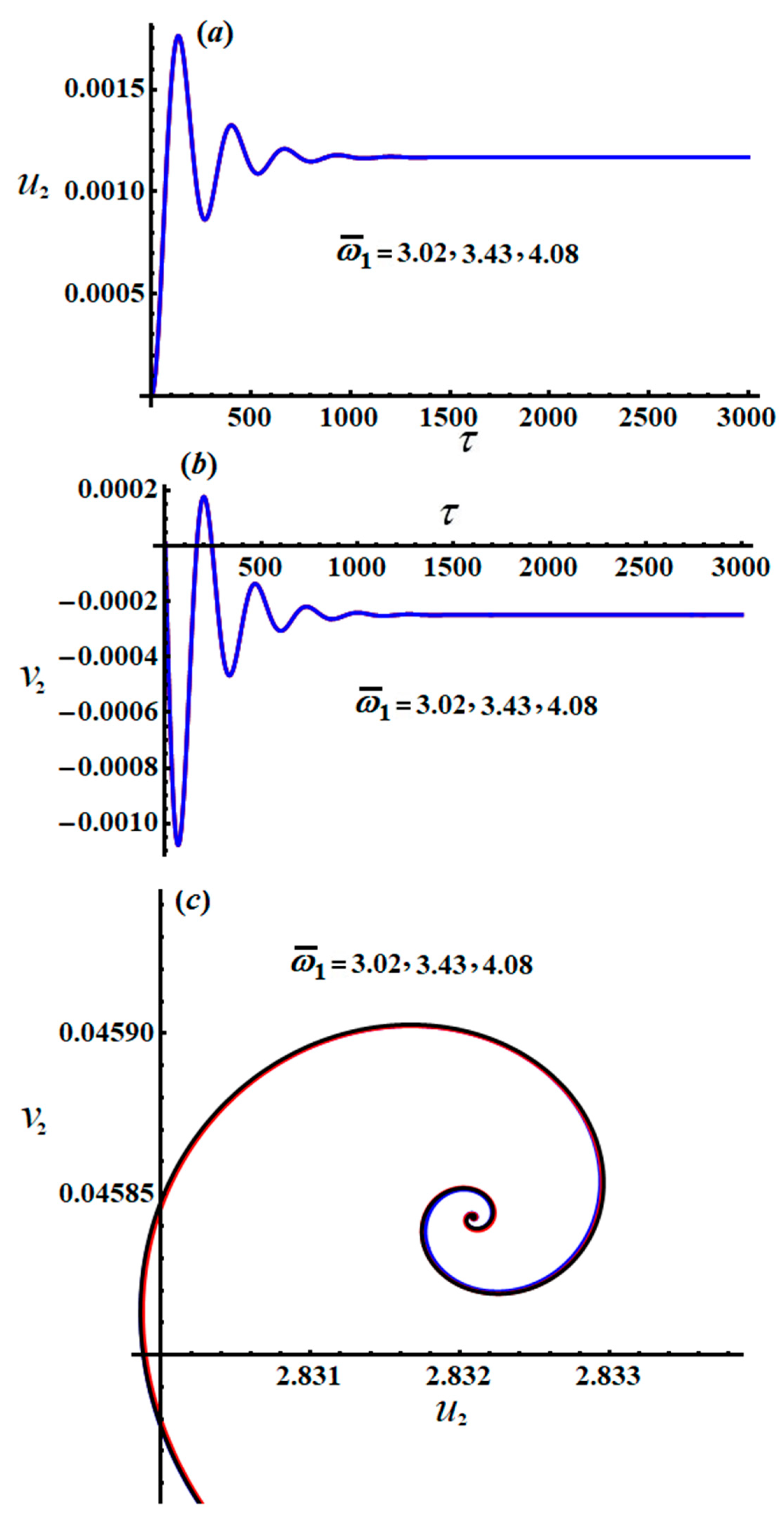
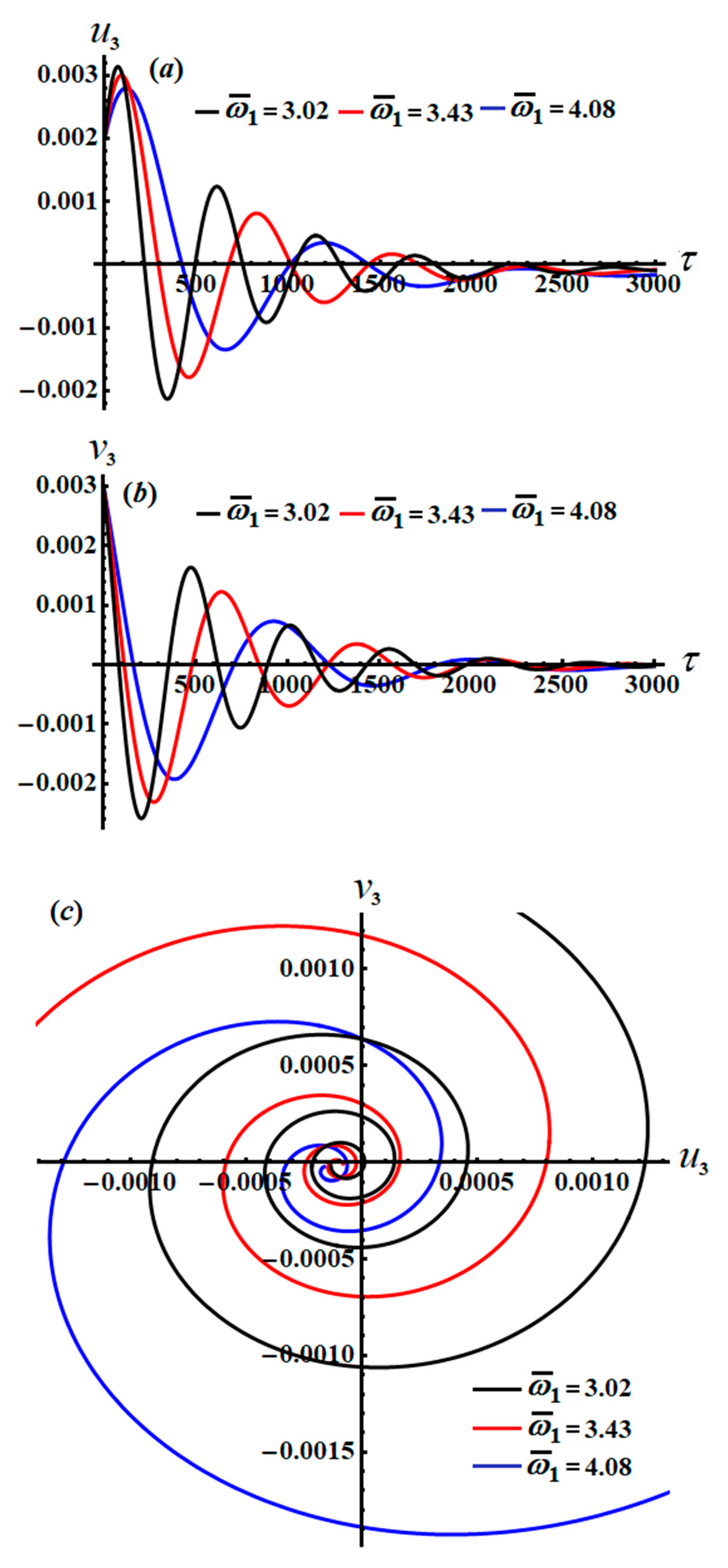
The inspection of parts of Figure 15 and Figure 18 shows the time histories of $u_1,v_1$ and the projections of the modulation equation trajectory on the phase plane $u_1{v}_1$. It is clear that $u_1,v_1$ and $u_1{v}_1$ increase gradually when time increases, and they behave in the form of a straight line due to the system of Equation (54). Conversely, the decay behavior of the waves describing the variation of $u_2,\hspace{0.17em}{v}_2,u_3$, and $v_3$ is shown in Figure 16a,b, Figure 17a,b, Figure 19a,b, and Figure 20a,b, for different values of ${\overline{\omega }}_1$ and ${\overline{\omega }}_2$. Spiral curves are plotted in the planes $u_2{v}_2$ and $u_3{v}_3$ in Figure 16c. Figure 16c in line with the equations of the system of Equation (54).

6. Conclusions

This work focused on the dynamical motion of a novel three DOF auto-parametric system consisting of the main motion of a non-linear Duffing oscillator and the secondary motion of a spring pendulum. The governing EOM of the system were obtained using Lagrange’s equations and solved using PTMS up to the third approximation. The solvability conditions and the equations of the modulations were obtained in view of the examined primary external resonance case. The curves of time histories and resonance were drawn, taking into consideration the selected values of some data. The non-linear analysis of the solutions in the steady state was presented and interpreted. The stability and instability areas were plotted to clarify their corresponding regions. The properties of the non-linear amplitudes of the modulation system and their stabilities were clarified and examined. The achieved results of this work can be applied to deal with the vibration of swaying buildings and to reduce the vibration of rotor dynamics, as well as in the fields of mechanics and space engineering. These outcomes generalized those of previous works in [5,31] for the absence of an applied force and moment in the unstarched arm of a pendulum.

References

1. El-Barki, F.A.; Ismail, A.I.; Shaker, M.O.; Amer, T.S. On the motion of the pendulum on an ellipse. ZAMM 1999, 79, 65–72. [Google Scholar] [CrossRef]
2. Leven, R.W.; Koch, B.P. Chaotic behavior of a parametrically excited damped pendulum. Phys. Lett. A 1981, 86, 71–74. [Google Scholar] [CrossRef]
3. Leven, R.W.; Pompe, B.; Wilke, C.; Koch, B.P. Experiments on periodic and chaotic motions of a parametrically forced pendulum. Phys. D Nonlinear Phenom. 1985, 16, 371–384. [Google Scholar] [CrossRef]
4. Amer, T.S.; Bek, M.A. Chaotic responses of a harmonically excited spring pendulum moving in circular path. Nonlinear Anal. Real World Appl. 2009, 10, 3196–3202. [Google Scholar] [CrossRef]
5. Hatwal, H.; Mallik, A.; Ghosh, A. Non-linear vibrations of a harmonically excited autoparametric system. J. Sound Vib. 1982, 81, 153–164. [Google Scholar] [CrossRef]
6. Nayfeh, A.H. Perturbations Methods; WILEY-VCH Verlag GmbH and Co. KGaA: Weinheim, Germany, 2004. Available online: https://onlinelibrary.wiley.com/doi/book/10.1002/9783527617609 (accessed on 19 December 2021).
7. Miles, J. Resonance and symmetry breaking for the pendulum. Phys. D Nonlinear Phenom. 1988, 16, 252–268. [Google Scholar] [CrossRef]
8. Bryant, P.J.; Miles, J.W. On a periodically forced, weakly damped pendulum. Part 1: Applied torque. J. Austral. Math. Soc. Ser. B 1990, 32, 1–22. [Google Scholar] [CrossRef] [Green Version]
9. Bryant, P.J.; Miles, J.W. On a periodically forced, weakly damped pendulum. Part 2: Horizontal forcing. J. Austral. Math. Soc. Ser. B 1990, 32, 23–41. [Google Scholar] [CrossRef] [Green Version]
10. Bryant, P.J.; Miles, J.W. On a periodically forced, weakly damped pendulum. Part 3: Vertical forcing. J. Austral. Math. Soc. Ser. B 1990, 32, 42–60. [Google Scholar] [CrossRef] [Green Version]
11. Kapitaniak, M.; Perlikowski, P.; Kapitaniak, T. Synchronous motion of two vertically excited planar elastic pendula. Commun. Nonlinear Sci. Numer. Simulat. 2013, 18, 2088–2096. [Google Scholar] [CrossRef] [Green Version]
12. Warminski, J.; Kecik, K. Autoparametric vibrations of a nonlinear system with pendulum. Math. Problems Eng. 2006, 2006, 19. [Google Scholar] [CrossRef]
13. Starosta, R.; Kamińska, G.S.; Awrejcewicz, J. Parametric and external resonances in kinematically and externally excited nonlinear spring pendulum. Int. J. Bifurc. Chaos 2011, 21, 3013–3021. [Google Scholar] [CrossRef]
14. Starosta, R.; Kamińska, G.S.; Awrejcewicz, J. Asymptotic analysis of kinematically excited dynamical systems near resonances. Nonlinear Dyn. 2012, 68, 459–469. [Google Scholar] [CrossRef]
15. Amer, T.S.; Bek, M.A.; Hamada, I. On the motion of harmonically excited spring pendulum in elliptic path near resonances. Adv. Math. Phys. 2016, 2016, 15. [Google Scholar] [CrossRef] [Green Version]
16. Awrejcewicz, J.; Starosta, R.; Kamińska, G.S. Asymptotic analysis of resonances in nonlinear vibrations of the 3-DOF pendulum. Differ. Equ. Dyn. Syst. 2013, 21, 123–140. [Google Scholar] [CrossRef]
17. Amer, T.S.; Bek, M.A.; Abouhmr, M.K. On the vibrational analysis for the motion of a harmonically damped rigid body pendulum. Nonlinear Dyn. 2018, 91, 2485–2502. [Google Scholar] [CrossRef]
18. Amer, T.S.; Bek, M.A.; Abohamer, M.K. On the motion of a harmonically excited damped spring pendulum in an elliptic path. Mech. Res. Commun. 2019, 95, 23–34. [Google Scholar] [CrossRef]
19. El-Sabaa, F.M.; Amer, T.S.; Gad, H.M.; Bek, M.A. On the motion of a damped rigid body near resonances under the influence of harmonically external force and moments. Results Phys. 2020, 19, 103352. [Google Scholar] [CrossRef]
20. Bek, M.A.; Amer, T.S.; Almahalawy, A.; Elameer, A.S. The asymptotic analysis for the motion of 3DOF dynamical system close to resonances. Alex. Eng. J. 2021, 60, 3539–3551. [Google Scholar] [CrossRef]
21. Amer, T.S.; Bek, M.A.; Hassan, S.S. The dynamical analysis for the motion of a harmonically two degrees of freedom damped spring pendulum in an elliptic trajectory. Alex. Eng. J. 2022, 2, 1715–1733. [Google Scholar] [CrossRef]
22. Kamińska, G.S.; Awrejcewicz, J.; Kamiński, H. Resonance study of spring pendulum based on asymptotic solutions with polynomial approximation in quadratic means. Meccanica 2020, 56, 753–767. [Google Scholar]
23. Bek, M.A.; Amer, T.S.; Sirwah, M.A.; Awrejcewicz, J.; Arab, A.A. The vibrational motion of a spring pendulum in a fluid flow. Results Phys. 2020, 19, 103465. [Google Scholar] [CrossRef]
24. Amer, W.S.; Bek, M.A.; Abohamer, M.K. On the motion of a pendulum attached with tuned absorber near resonances. Results Phys. 2018, 11, 291–301. [Google Scholar] [CrossRef]
25. Song, Y.; Sato, H.; Iwata, Y.; Komatsuzaki, T. The response of a dynamic vibration absorber system with a parametrically excited pendulum. J. Sound Vib. 2003, 259, 747–759. [Google Scholar] [CrossRef]
26. Warminski, J.; Kecik, K. Instabilities in the main parametric resonance area of a mechanical system with a pendulum. J. Sound Vib. 2009, 322, 612–628. [Google Scholar] [CrossRef]
27. Warminski, J. Regular and chaotic vibrations of a parametrically and self-excited system under internal resonance condition. Meccanica 2005, 40, 181–202. [Google Scholar] [CrossRef]
28. Kecik, K.; Warminski, J. Dynamics of an autoparametric pendulum-like system with a nonlinear semiactive suspension. Math. Probl. Eng. 2011, 2011, 15. [Google Scholar] [CrossRef] [Green Version]
29. Kecik, K.; Mitura, A.; Warmiński, J. Efficiency analysis of an autoparametric pendulum vibration absorber. Eksploat. I Niezawodn.-Maint. Reliab. 2013, 15, 221–224. [Google Scholar]
30. Kecik, K.; Mitura, A. Energy recovery from a pendulum tuned mass damper with two independent harvesting sources. Int. J. Mech. Sci. 2020, 174, 105568. [Google Scholar] [CrossRef]
31. Brzeski, P.; Perlikowski, P.; Yanchuk, S.; Kapitaniak, T. The dynamics of the pendulum suspended on the forced Duffing oscillator. J. Sound Vib. 2012, 331, 5347–5357. [Google Scholar] [CrossRef] [Green Version]
32. Gantmacher, F.R. Applications of the Theory of Matrices; John Wiley & Sons: New York, NY, USA, 2005. [Google Scholar]
33. Amer, T.S.; Bek, M.A.; Hassan, S.S.; Elbendary, S. The stability analysis for the motion of a nonlinear damped vibrating dynamical system with three-degrees-of-freedom. Results Phys. 2021, 28, 104561. [Google Scholar] [CrossRef]
34. Abady, I.M.; Amer, T.S.; Gad, H.M.; Bek, M.A. The asymptotic analysis and stability of 3DOF non-linear damped rigid body pendulum near resonance. Ain Shams Eng. J. 2022, 13, 101554. [Google Scholar] [CrossRef]
35. Abohamer, M.K.; Awrejcewicz, J.; Starosta, R.; Amer, T.S.; Bek, M.A. Influence of the motion of a spring pendulum on energy-harvesting devices. Appl. Sci. 2021, 11, 8658. [Google Scholar] [CrossRef]
36. Amer, W.S.; Amer, T.S.; Hassan, S.S. Modeling and stability analysis for the vibrating motion of three degrees-of-freedom dynamical system near resonance. Appl. Sci. 2021, 11, 11943. [Google Scholar] [CrossRef]
37. Amer, W.S.; Amer, T.S.; Starosta, R.; Bek, A.M. Resonance in the cart-pendulum system-an asymptotic approach. Appl. Sci. 2021, 11, 11567. [Google Scholar] [CrossRef]
38. Amer, T.S.; Starosta, R.; Elameer, A.S.; Bek, M.A. Analyzing the stability for the motion of an unstretched double pendulum near resonance. Appl. Sci. 2021, 11, 9520. [Google Scholar] [CrossRef]
39. Abdelhfeez, S.A.; Amer, T.S.; Elbaz, R.F.; Bek, M.A. Studying the influence of external torques on the dynamical motion and the stability of a 3DOF dynamic system. Alex. Eng. J. 2022, 61, 6695–6724. [Google Scholar] [CrossRef]
Figure 1. Description of the system.
Applsci 12 01737 g001
Figure 2. The amplitude’s modulation h 1 and modified phase θ 1 : (a,b) at ω ¯ 1 = ( 3.02 , 3.43 , 4.08 ) , (c,d) at ω ¯ 2 = ( 4.43 , 5.72 , 6.68 ) , (e,f) at ω ¯ 3 = ( 7.07 , 7.75 , 8.37 ) .
Applsci 12 01737 g002
Figure 3. The variation of h 2 and θ 2 with τ : (a,b) at ω ¯ 1 = ( 3.02 , 3.43 , 4.08 ) , (c,d) at ω ¯ 2 = ( 4.43 , 5.72 , 6.68 ) , (e,f) at ω ¯ 3 = ( 7.07 , 7.75 , 8.37 ) .
Applsci 12 01737 g003
Figure 4. The time histories of the amplitude h 3 and the phase θ 3 : (a,b) at ω ¯ 1 = ( 3.02 , 3.43 , 4.08 ) , (c,d) at ω ¯ 2 = ( 4.43 , 5.72 , 6.68 ) , (e,f) at ω ¯ 3 = ( 7.07 , 7.75 , 8.37 ) .
Applsci 12 01737 g004
Figure 5. The change of the attained Y , X , and ϕ with time τ : (ac) when ω ¯ 1 = ( 3.02 , 3.43 , 4.08 ) .
Applsci 12 01737 g005
Figure 6. The time histories of the approximate solutions Y , X , and ϕ : (ac) when ω ¯ 2 = ( 4.43 , 5.72 , 6.68 ) .
Applsci 12 01737 g006
Figure 7. The variation of Y , X , and ϕ versus τ : (ac) when ω ¯ 3 = ( 7.07 , 7.75 , 8.37 ) .
Applsci 12 01737 g007
Figure 8. The amplitude modulation of h 1 , h 2 , h 3 as a function of θ 1 , θ 2 , θ 3 : (ac) at ω ¯ 1 = 4.08 .
Applsci 12 01737 g008
Figure 9. The amplitude modulation of h 1 , h 2 , h 3 as a function of θ 1 , θ 2 , θ 3 : (ac) at ω ¯ 2 = 5.72 .
Applsci 12 01737 g009
Figure 10. The amplitude modulation of h 1 , h 2 , h 3 as a function of θ 1 , θ 2 , θ 3 : (ac) at ω ¯ 3 = 8.37 .
Applsci 12 01737 g010
Figure 11. The change of the frequency responses of h 1 , h 2 , h 3 with σ 1 at σ 2 = 0 , σ 3 = 0 : (ac) when ω ¯ 1 = ( 3.02 , 3.43 , 4.08 ) .
Applsci 12 01737 g011
Figure 12. The variation of the frequency response h 1 with σ 1 at σ 2 = 0 , σ 3 = 0 when ω ¯ 2 = ( 4.43 , 5.72 , 6.68 ) .
Applsci 12 01737 g012
Figure 13. The variation of the frequency response h 2 with σ 1 at σ 2 = 0 , σ 3 = 0 when ω ¯ 2 = ( 4.43 , 5.72 , 6.68 ) .
Applsci 12 01737 g013
Figure 14. The variation of the frequency responses h 3 with σ 1 at σ 2 = 0 , σ 3 = 0 when ω ¯ 2 = ( 4.43 , 5.72 , 6.68 ) .
Applsci 12 01737 g014
Figure 15. The modified amplitudes via τ and the projections of the modulation equation tracks on the phase plane u 1 v 1 : (ac) when ω ¯ 1 = ( 3.02 , 3.43 , 4.08 ) .
Applsci 12 01737 g015
Figure 16. The modified amplitudes via τ and the projections of the modulation equation tracks on the phase plane u 2 v 2 : (ac) when ω ¯ 1 = ( 3.02 , 3.43 , 4.08 ) .
Applsci 12 01737 g016
Figure 17. The modified amplitudes via τ and the projections of the modulation equation tracks on the phase plane u 3 v 3 : (ac) when ω ¯ 1 = ( 3.02 , 3.43 , 4.08 ) .
Applsci 12 01737 g017
Figure 18. The modified amplitudes via τ and the projections of the modulation equation tracks on the phase plane u 1 v 1 : (ac) when ω ¯ 2 = ( 4.43 , 5.72 , 6.68 ) .
Applsci 12 01737 g018
Figure 19. The modified amplitudes via τ and the projections of the modulation equation tracks on the phase plane u 2 v 2 : (ac) when ω ¯ 2 = ( 4.43 , 5.72 , 6.68 ) .
Applsci 12 01737 g019
Figure 20. The modified amplitudes via τ and the projections of the modulation equation tracks on the phase plane u 3 v 3 : (ac) when ω ¯ 2 = ( 4.43 , 5.72 , 6.68 ) .
Applsci 12 01737 g020
Publisher’s Note: MDPI stays neutral with regard to jurisdictional claims in published maps and institutional affiliations.