Article

Effect of Formation Size on Flocking Formation Performance for the Goal Reach Problem

1
Department of Computer Science, College of Computer and Information Sciences, King Saud University, Riyadh 11362, Saudi Arabia
2
Computer Engineering Department, Al Yamamah University, Riyadh 11512, Saudi Arabia
*
Author to whom correspondence should be addressed.
Appl. Sci. 2022, 12(7), 3630; https://doi.org/10.3390/app12073630
Submission received: 22 February 2022 / Revised: 26 March 2022 / Accepted: 31 March 2022 / Published: 3 April 2022
(This article belongs to the Special Issue Robotics in Life Science Automation)

Abstract

:
Flocking is one of the swarm tasks inspired by animal behavior. A flock involves multiple agents aiming to achieve a goal while maintaining certain characteristics of their formation. In nature, flocks vary in size. Although several studies have focused on the flock controller itself, less research has focused on how the flock size affects flock formation and performance. In this study, we address this problem and develop a simple flock controller for goal-zone-reaching tasks. The developed controller is intended for a two-dimensional environment and can handle obstacles as well as integrate an additional invented feature, called sensing power, in order to simulate the natural dynamics of migratory birds. This controller is simulated using the NetLogo simulation tool. Several experiments were conducted with and without obstacles, accompanied by changes in the flock size. The simulation results demonstrate that the flock controller is able to successfully deliver the flock to the goal zone. In addition, changes in the flock size affect multiple metrics, such as the time required to reach the goal (and, consequently, the time required to complete the flocking task), as well as the number of collisions that occur.

1. Introduction

Many researchers have focused on robotic swarms—robot groups that co-operate to achieve a global goal in a complex environment [1]. The flocking problem, inspired by the behavior of animals (e.g., birds flocking or fish schooling), is a subfield of swarm robotics [2]. A swarm consists of a set of similar members having the same characteristics and progressing in an asynchronous manner. There is no leader in the swarm directing other members to perform the planned tasks. Thus, a swarm operates in a decentralized context, where complex behavior arises through the labor of autonomous agents that are acting on local information. An agent cannot conclude the swarm aims without collaborating with the rest of the group [3]. One of the main components of a swarming system is the exhibition of cooperative behavior. A flock involves multiple agents that possess real-time group behavior capabilities that facilitate achieving a common target, such as foraging or migration [4,5]. The design of swarm robotics systems is guided by swarm intelligence principles. Brambilla [6] divided the swarm behaviors into four major categories—spatial organization, navigation, decision making, and miscellaneous—each of which has different areas of application. Schranz [7] proposed an extension to the categorization of the basic swarm behaviors. They used this taxonomy to classify a number of existing swarm robotic applications from research and industrial domains. Several studies were orientated towards modeling swarm robots to increase the understanding of natural swarm systems [8]. In a robotic swarm, the collective behavior results from local interactions among the robots and between the robots and the environment. One area that researchers have investigated is the study of the efficiency in self-regulation of swarms of birds, schools of fish, and social insect colonies, whereas others initiated models to generate and optimize artificial swarm systems as engineered in the field of swarm robotics  [9]. One can notice the importance of models that suggest novel empirical experiments, as well as the prominence of empiric experimentation that results in relevant model parameterizations  [10]. Dias et al. [8] published an extensive review presenting a discourse on a large panoply of features, covering swarm robotics.
The individual elements in such flocks move, while maintaining specific velocities and distances among each other without splitting. Reynolds [11,12] has specified three fundamental flocking rules: collision avoidance, flock centering, and velocity matching (alignment). Animal groups change their structure depending on internal or external stimuli, thus maximizing the fitness of individuals as circumstances change [13]. The behavior of these agents, integrated within the structural order, results in changes of direction and shape without affecting the group’s coherence [13].
Formation control aims to produce control commands that are sufficient to drive multiple agents to reach their status constraints [4]. To endow self-organization systems with flexibility and robustness, controllers use decentralized mechanisms [14]. A controller is an essential structure that is used in the implementation and simulation of swarm systems [15]. There are three main approaches to formation control systems [4,12,16]: the leader–follower approach [12,17,18,19], the virtual structure approach [1,20,21], and the behavior-based approach [5,14,16,22,23,24,25,26]. Despite the simplicity of the leader–follower approach, it may suffer from being highly dependent on the leader agent and from the large amount of information exchange required between the leader and each of the followers due to being a centralized system [4]. Moreover, virtual structure approaches lack formation modification when the formation changes due to structural redesign, which increases the required computation and degrades collision avoidance abilities. On the other hand, the behavior-based approach allows for the handling of multiple tasks using a single controller [4]. Notably, in the literature, most researchers have used the behavior approach, due to the fact that the flocking task is usually directly inspired by natural animal behavior.
The flock size is the number of individuals within the flock. In nature, animals tend to have higher survival rates when being part of a group. In fact, group size is one of the primary defense mechanisms that animals adopt in order to limit predation risks [27,28]. The size of a flock in nature can range from one species to hundreds of different species. Accordingly, flocking applications use different flock sizes, based on the application objectives [29]. As the flock size increases, the rate of successful attacks decreases [30]. Nevertheless, there are several disadvantages to grouping [30], including greater competition between group members and greater exposure to predators. On the other hand, some of the advantages of grouping are foraging, defense, alertness, and risk reduction [27,31].
Indeed, flock size is one of the main behavioral mechanisms used by animals to manage their vulnerability to predation. Hintz et al. [32] studied the direct effect of flock size on foraging success with respect to the predation risk. Cresswell  [30] investigated how the flock size risk thresholds differ for attack rate, success rate, or dilution. The optimal flock size reflects a dynamic interplay between a diverse range of costs (competition, visibility, etc.) and benefits (defense, vigilance, etc.) associated with joining a group  [27].
Most research has focused on constructing new methods or enhancing existing methods related to flock formation and control. Consequently, fewer efforts have been made in studying the effects of flocking parameters, such as flock size, on the performance of the developed systems. Zhang et al. [26] have studied the impact of changing flock size on reaching the goal in a specific time. They conducted two types of experiments; the first one was applied to test their work, with the objective of reaching the goal in a fixed time. For this experiment, they used 30 robots, and found that the flock could converge within a specific time. The second experiment focused on showing the effect of converging time when the flock size changed, with experiments using 2 , 4 , 6 , , 40 robots. They concluded that the convergence time decreases as the number of agents increases. Moreover, Márquez et al. [14] have used three types of experiments to test (i) the cooperative behavior, (ii) the optimized control parameters, and (iii) the objective functions, when using 5, 10, or 20 agents. They found that the number of agents and the existence of obstacles did not affect the flock’s performance. Moreover, the performance of the flock was improved when the repulsion zone was small, and the orientation and attraction zones were large. Figure 1 depicts these three different zones. The flock direction in the proposed work was decided in consensus between the different agents. Therefore, they found that the complexity of the determined direction increases as the flock size increases. The importance of the orientation radius also increased as the flock size increased. On the other hand, Olfati [23] has proposed different algorithms to simulate and study the flock behavior, according to their number and distribution in free space and with obstacles. However, these works did not study how the flock size affects the formation, whether the flock size affects the time it takes to reach the goal, whether all agents successfully reach the goal, how much time the flock takes to match the velocity, and whether the flock maintains the flocking roles while exploring.
In this paper, we study the relationship between flock size and its effect on the flocking system’s formation and performance. Inspired by previous works [13,14,16], a flocking system is constructed. Performance is measured according to a number of factors, including the flexibility towards reaching the goal (e.g., the time to reach the goal zone, number of agents within the goal area), time to match the velocity, the number of applied flocking rules (e.g., separation, cohesion, and alignment), and the number of collisions that occur. Additional parameters are taken into account, such as the average distance to the center of mass, goal localization time, and localization window.

2. Materials and Methods

The objective of this study is to evaluate the performance of a flock during a flocking task with an unknown target zone. The tasks tackled in this paper are similar to those in the studies [13,14,16]. However, this study is characterized by the objective functions it defines, along with the various metrics used to analyze and evaluate the performance and behavior of the controller.

2.1. Assumptions

The controller developed in this paper is based on an existing controller [14]. Some features are used, such as the repulsion zone, attraction zone, orientation zone, and the view sectors of the agent, while others are added, such as the sensing power to replicate the migration of birds in nature. Completion of the task is determined when all agents reach the goal zone. First, some assumptions about the controller need to be highlighted—these assumptions also represent the controller’s boundaries.
  • The system is deployed in a two-dimensional geographical region;
  • Obstacles in the environment are static obstacles;
  • The arena size always fits the agents. It includes the initial zone and the goal zone;
  • The environment has a static goal located within the goal zone, which is a circular region with a center, ( g x , g y ) , and a radius, r g ;
  • The initial zone is a circular region with a radius, r z ;
  • Agents are homogeneous;
  • The positions of the agents are randomly generated within the initial zone;
  • The velocity of each agent is initially random, within a bounded range, ( v m i n , v m a x ) ;
  • The direction of each agent is initialized randomly;
  • Each agent can sense its neighbors within a maximum distance with radius Δ a , as shown in Figure 1, from its position;
  • There exists a sensing power, which works as a hint towards the goal position (see Section 2.5).

2.2. Flock Design and Representation

The proposed flock controller’s design is inspired by previous studies [13,14], where each agent is able to sense other neighbors and obstacles within three zones: the zone of repulsion, z o r , with width Δ r ; the zone of orientation, z o o , with width Δ o ; and the zone of attraction, z o a , with width Δ a (see Figure 1a). Each agent has several view sectors (in this case, eight sectors), S i = [ u ^ 1 , u ^ 2 , , u ^ 8 ] T , where u ^ k = [ cos ( ( 2 k 1 ) × π 8 ) sin ( ( 2 k 1 ) × π 8 ) ] , as shown in Figure 1b. These view sectors are used to locate an agent within ( 0 , 2 π ) radii. Agents then behave depending on the surrounding environment and their neighbors.

2.3. Behavior of Agents

Each agent behaves based on its surrounding environment and neighbors within the perception zones. Each agent, i, has a number of vectors that help to determine its direction. These vectors are as follows:
  • A goal-zone-detection vector, V g i = [ v g i , 1 , v g i , 2 , , v g i , 8 ] T , where each v g i , k is equal to 1 if a goal is detected in view sector k of agent i, within its perception area ( z o a ), and is equal to zero otherwise. The unit vector d g i , which denotes the desired direction of agent i based on the goal detected, is calculated as follows: d g ^ i = s i v g ˙ i s i v g ˙ i .
  • An obstacle-detection vector, V b i = [ v b i , 1 , v b i , 2 , , v b i , 8 ] T , where each v b i , k is equal to 1 if an obstacle is detected in view sector k of agent i within its perception area, and is equal to zero otherwise. The unit vector d b i , which denotes the desired direction of agent i based on the opposite net direction of obstacles detected, is calculated as follows: d b ^ i = s i v b ˙ i s i v b ˙ i .
  • An arena-exploration unit vector, d e i ^ = [ cos ( θ r a n d , i ) sin ( θ r a n d , i ) ] , is required, in order to help the agent explore the unknown environment. This vector has a single value: a random angle in the range θ r a n d , i ( 0 , 2 π ) . In the case where an obstacle has been detected, the angle is modified to θ r a n d , i ( 0 , π ) , such that the agent heads towards a region in the opposite direction of the observed obstacle.
On the other hand, agents also have to consider their neighbors, in order to avoid collisions with each other, as well as maintaining the coherence of the flock, to avoid fragmentation, and to keep the agents aligned. Therefore, agents have another three vectors defining how they behave, according to their nearby neighbors. These vectors are defined according to the three zones ( z o r , z o o , and z o a ) for each agent i, as follows:
  • A repulsion zone vector V r i = [ v r i , 1 , v r i , 2 , , v r i , 8 ] T . This vector allows for the detection of neighbors in the repulsion zone of agent i. The existence of one or more neighbors in view sector k of agent i is represented by a 1 in v r i , k , whereas their absence is represented by a 0. The corresponding unit vector is calculated as d r i ^ = s i v r ˙ i s i v r ˙ i .
  • For each neighbor, j, detected in z o o of agent i, having a travel direction represented as θ j , the unit vector ( o j ) ^ = [ cos ( θ j ) sin ( θ j ) ] stores the direction of travel of this neighbor. The unit vector with a size equal to the number of neighbors n 0 in z o o , which is responsible for alignment with other agents in the flock, is given by d o i ^ = j = 1 n 0 o j ^ j = 1 n 0 o j ^ .
  • The attraction zone vector, V a i = [ v a i , 1 , v a i , 2 , , v a i , 8 ] T . v a i , k , is assigned a value of 1, based on the existence of one or more neighbors in the view sector k of agent i, and is assigned as 0 otherwise. The corresponding unit vector is calculated as d a i ^ = s i v a ˙ i s i v a ˙ i , which determines the direction of far neighbors in the z o a , in order to avoid fragmentation of the flock.

2.4. Computing the Final Desired Direction

After calculating each vector’s desired direction, each agent must have a single direction ( d i ) to move towards. The final desired direction is determined according to the sensed positions of neighboring agents and the current environment status (goal and obstacles).
In the case that neighbors are detected in the repulsion zone, the final desired direction is computed according to Equation (1) [14]. For example, Equation (1a) indicates that, in the case that obstacles are detected in addition to the goal zone, then the function computing d i will guide the agent away from neighbors ( d r i ^ ) and obstacles ( d b i ^ ), but also towards the goal ( d g i ^ ). Note that the exploration capability ( d e i ^ ) is only activated in the absence of goal detection (Equations (1c,d)). Márquez-Vega et al. [14] have used three weights, w 1 , w 2 , and w 3 , such that avoiding collisions between neighbors was assigned higher priority than that of alignment and cohesion. The sensing power feature and conditions (Equation (1e)) are explained in Section 2.5.
d i = w 1 d r i ^ + w 2 d b i ^ + w 3 d g i ^ , goal zone and obstacle detected ( a ) w 1 d r i ^ + ( w 2 + w 3 ) d g i ^ , goal zone detected ( b ) w 1 d r i ^ + w 2 d b i ^ + w 3 d e i ^ , obstacle detected ( c ) w 1 d r i ^ + ( w 2 + w 3 ) d e i ^ , agents detected in z o r . ( d ) s p i ^ , conditions for sensing power satisfied ( e )
If no neighbors are detected in the repulsion zone, then the final desired direction will be computed according to Equation (2). Note that the alignment and orientation capabilities are used only in the absence of neighbors in the repulsion zone [13].
d i = d o i ^ + d a i ^ + d b i ^ + d g i ^ , goal zone and obstacle detected ( a ) d o i ^ + d a i ^ + d g i ^ , goal zone detected ( b ) d o i ^ + d a i ^ + d b i ^ + d e i ^ , obstacle detected ( c ) d o i ^ + d a i ^ + d e i ^ , other agents detected in perception zone ( d ) s p i ^ , conditions for sensing power satisfied ( e )

2.5. Sensing Power

In nature, members of a flock usually know where they are heading, even if they do not precisely know their goal location. Therefore, we propose the sensing power, which acts as the effect of such knowledge on the flock’s heading direction, and which is added to the flock controller. This sensing power allows the flock to take off better and gives the controller a more natural flock characteristic. Moreover, it helps lost or late agents to integrate the flock quickly by assisting them to orient themselves towards the center of mass of the flock. Indeed, an agent, in their way with the flock, can encounter several obstacles. By avoiding these obstacles, they can move away from the flock and lose the flock heading direction; thus, they have to rely on their senses. In this case, the sensing power is triggered to direct the agent towards the flock. Based on the limitations of the simulation arena’s size, we decided to apply this sensing power only in the initial period, such that it does not cause guided flocking behavior.
The sensing power is represented by a vector comprising two angles of direction illustrating the fields of attraction of the objective. The objective is a circle with center, C, and radius, r. This circle may represent either the target zone or the flock. Figure 2 depicts the principle of the attraction field of the sensing power.
Let us consider that an agent is in position, P 0 . The attraction field of the objective is then delimited by P 0 and two points of tangency ( P 1 , P 2 say) in the circle (i.e., the objective)—where ( P 0 , P 1 ) defines a first line that is tangent to the circle and ( P 0 , P 2 ) defines a second line that is also tangential to the circle. The agent has the freedom to move inside this field of attraction. Let us denote:
  • θ = ( P 2 P 0 P 1 ) : the angle in P 0 , defined by the triplet ( P 2 , P 0 , P 1 ) (Equation (3)),
    θ = 2 × tan 1 ( r d 2 r 2 )
  • ϕ = ( ( P 0 , C ) , X a x i s ) : the angle in P 0 , defined by the two lines ( P 0 , C ) and X a x i s (Equation (4)),
    ϕ = arctan 2 ( C y P 0 y , C x P 0 x )
  • d = P 0 C the Euclidean distance between P 0 , the location of the agent, and C, the center of the objective. One can notice that the agent may choose randomly a direction angle, θ r a n d , so that θ r a n d [ ϕ θ / 2 , ϕ + θ / 2 ] (Equation (5)).
    θ r a n d = r a n d o m ( ϕ θ / 2 , ϕ + θ / 2 )
The sensing power is represented as vector of two direction angles s p i = [ ϕ , θ ] T , where their combination characterizes the opening angle of the field of attraction sector (blue sector in Figure 2). Applying this sensing power with a random angle accordingly allows the agent to proceed towards their objective (Equation (6)).
s p i ^ = θ r a n d , if the sensing power is triggered 0 , otherwise

2.6. Flock Controller Algorithm

The proposed flock controller algorithm (Algorithm 1) shows the flock controller’s basic steps, and illustrates when the sensing power is used.
Algorithm 1:Flock Controller.
Applsci 12 03630 i001
The flock controller starts by determining the goal position and its radius, as well as the initial zone and its radius. After that, n agents are generated, with random position, direction, and velocity, within the initial zone. Velocities are bounded with minimum and maximum values ( v m i n , v m a x ) , thus avoiding high differences between the velocities of agents, which may cause flock fragmentation. As these agents are generated, each agent checks whether its randomly selected position is not already taken by another agent, such that no two agents have the same position. Then, the agents start exploring. If the flock task has just started, then each agent finds the sensing power angle and determines the final desired direction. Then, all agents begin to move. Otherwise, they must find the final desired direction for each agent and then move. Meanwhile, each agent checks whether it is within the goal zone area or explores the arena. If all agents are within the goal zone area, the flock controller is terminated.
Moreover, while the flock controller is processing, some outputs are generated, such as the number of agents within the goal area, the time to match the velocity, the number of applied flocking rules, the number of occurred collisions, the localization time, and the distance to the center of mass. When the flock’s task is completed, the flock controller is terminated and the time to reach the goal zone is determined, as well as the localization window. These outputs are used to test the model’s performance.

2.7. Performance Metrics

The performance metrics use the time steps taken by the flock as a measurement unit. To study the effect of the flock size on the flock’s performance, in terms of completing the task of reaching a goal zone, the algorithm outputs the following metrics. Table 1 summarizes the notation used.
  • Number of agents within the goal area. Each agent i has a status variable, g i (Equation (7)), which checks at every step whether agent i is in the goal zone or not.
    g i = 1 , goal zone detected by agent i 0 , otherwise
  • Time to reach the goal zone: This metric provides the minimum number of steps taken by at least one of the flock agents to reach the goal zone. In other words, the number of steps for the first agent i to achieve g i = 1 .
  • Time required to complete the flocking task: This metric provides the actual time (in minutes) from the start of the simulation until the last agent enters the goal zone.
  • Speed matching time: This metric provides the minimum number of steps taken by the flock to match the speeds of all of its agents.
  • Localization window: This metric provides the difference in the number of steps from the time the first agent enters the goal zone until the last agent does.
  • Number of applying flocking rules (collision avoidance “separation”, attraction “cohesion”, and alignment) per agent, as defined in Equations (8)–(10):
    s e p a r a t i o n s = 1 n s = 1 T s e p s ,
    a l i g n m e n t s = 1 n s = 1 T a l s ,
    c o h e s i o n s = 1 n s = 1 T c o s .
In addition to these metrics, some objective functions used in ref. [14] are used as well, as follows:
  • Goal zone localization time: The average number of steps to localize the goal zone by every member of the flock (Equation (11)).
    l o c a l i z a t i o n T i m e = 1 n i = 1 n s i
  • Average distance to the center of mass (Equation (12)), where the average center of mass of the flock at each step, s, is defined by Equation (13):
    d i s t a n c e T o C o M = 1 T s = 1 T 1 n i = 1 n d ( c s , r i , s ) ,
    c s = 1 n i = 1 n r i , s .
  • Collisions per member. This metric reports the number of collisions that occurred between agents and obstacles. The number of collisions a s among all flock agents i, j at step s is computed based on the distances between them in D s (Equation (14)), according to Equation (15).
    D s = 0 d 12 d 1 n d 21 0 d 2 n d n 1 d n 2 0 ,
    a s = a s + 1 , d i j d c , d i j D s , 1 i < j n a s , otherwise .
    Then, the collisions between agent i n and obstacles at step s are computed, as in Equations (16)–(18). Finally, the average number of collisions among the flock members and with obstacles is computed, as in Equation (19).
    o i = 1 , obstacle detected within collision distance of agent i 0 , otherwise ,
    o s = [ o 1 , o 2 , , o n ] ,
    b s = i = 1 s o i , o i o s ,
    c o l l i s i o n s = 1 T s = 1 T a s + b s .

3. Results

3.1. Simulation Environment

The flock controller’s experimental setups consisted of different combinations between swarm sizes and arena conditions. According to [14], the used arena size should be 50 × 50 m for flock sizes between 5 and 20 agents. The initial zone was 10 × 10 m, and the goal zone had a radius of 10 m. However, these specifications were used for a maximum of 20 agents in the flock and may not be suitable when scaling up the flock size. Therefore, we considered the ratio between these specifications to scale the arena, based on the flock size. As such, the arena size could be represented as 100 % of the space, the initiating zone may be represented as 4 % , and the goal zone about 12.6 % of the arena size (according to the circle area A = π r 2 , as shown in Figure 3). These ratios were used in the experiments, regardless of the position of the initial and goal zones. In contrast to [14], we assumed that the initial zone had a circular shape, but still used the same ratio in the initial zone specifications.
Scaling up the arena requires more specification, in order to determine its size. Suppose that each agent occupies a 1 m 2 size of the arena; this allows the maximum required space for an agent to be 50 × 50 20 = 125 m 2 of the arena’s space. Therefore, using the proper ratio to calculate the suitable space of the arena is achieved by multiplying the maximum flock size by 125. In this work, we conducted experiments with flock sizes in the range of 10 100 agents in steps of 10. To ensure the containment of agents and obstacles, and to have a standard environment for comparison, the arena specifications for the maximum flock size (100 agents) will be considered as follows: The arena size was 112 × 112 m, the radius of the initial zone was 13 m, and the goal zone’s radius was 22 m. The experimental parameters are summarized in Table 2.
Tools known as agent-based modeling and simulation (ABMS) tools help researchers to understand the desired model through the simulation of real-world scenarios [33,34]. These tools use a shared environment, in which agents communicate and interact dynamically with each other [34]. Different ABMS tools have been developed to serve different problem fields. NetLogo [35] has an easy-to-use interface and is capable of simulating complex phenomena [33]. We used NetLogo version 6.2.0 as a simulation tool, on a macOS machine with 2 GHz and 16 GB RAM. NetLogo is based on two concepts representing the simulation world: patch and turtle. The patch represents the world’s grid, as shown in Figure 4. On the other hand, turtles are agents who move around the world. The world is split into a grid of patches, and is two-dimensional. Turtles may move across patches, described as square pieces of “ground”. The patch size was set as 5.5 × 5.5 pixels. Agents were set to fit a single patch size. On the other hand, the size of obstacles varied between one to two patches [23]. Obstacles were added manually, as adding obstacles randomly to the arena may lead to scenarios where the flock never applies obstacle avoidance. Collisions were considered to occur when the distance between two agents (or an agent and an obstacle) was less than d c = 0.55 .
A time step does not directly map to real-world time (seconds). In our simulation, each time step varied between 0.095 and 0.973 s, based on the step length taken by the simulation code. Therefore, we suppose that the time step interval is 1 s. Each agent initially has a random speed. This random speed is assumed to be a floating number between 0 and 0.5. Hence, the movement of the agent could not exceed 0.5 patches ahead.
In contrast to [14], where various perception zones were used, we conducted multiple tests to determine suitable common perception zones for all experimented flock sizes. Several zone sizes ( Δ r , Δ o , and Δ a ) were tested on flock sizes of 30, 50, and 100 agents. Agent perception zone sizes were selected based on the results of these tests. The test results considered goal zone localization time, the average distance to the center of mass, collisions per member, and the applied times of flocking rules. According to [14], a smaller value of Δ r , and larger values of Δ o and Δ a led to better flocking behavior. However, there were no precise ratios or constraints on the total perception radii. Therefore, a number of zone sizes were tested (e.g., Δ r = 2 , Δ o = 6 , and Δ a = 7 for 30 agents) where the flock did not show stable flocking behavior. To the contrary, the flock kept avoiding collision between its members and maintained cohesion simultaneously. Therefore, we eliminated the sizes that caused a similar situation from the next test on bigger flock sizes (detailed results provided in Appendix A). Experimentally, we found that smaller values of Δ r and Δ a , and larger values of Δ o led to better flocking behavior. The final selected zones were the minimum common sizes among all flock sizes that provided stable flocking behavior ( Δ r = 1 , Δ o = 13 , Δ a = 1 ) . According to the arena specifications set earlier, the agent’s perception area covered 5.5 % of the arena’s size. The repulsion priority weights w 1 , w 2 , and w 3 (Equation (1)) were set according to reference [14] to allow for improved repulsion behavior and to avoid having the desired position be too far from the agent, as follows: w 1 = 0.4 , w 2 = 0.75 , and w 3 = 0.025 .

3.2. Experimental Results

Each experiment was simulated 20 times (for 400 experiments in total) using NetLogo, and the obtained performance measures for each simulation were recorded. We report the average values obtained for each of the performance metrics over the twenty runs. Performance metric data for all simulations were analyzed using SPSS software [36].
Our aim is to explore the existence of an association between the change in flock size (as an independent variable) and each of the performance measures (as dependent variables).
  • We use regression curves to approximate the function or curve that has the best fit to a number of observed data points in our experiments [37,38,39].
  • The correlation coefficient, r [ 1 , 1 ] , describes the relationship and measures the strength of the association between two variables, and is defined in Equation (20) [40], where m is the sample size (i.e., the number of experiments), x is the value of the independent variable (i.e., the flock size), and y is the value of the dependent variable (i.e., the performance metric).
  • The coefficient of determination, R 2 [ 0 , 1 ] , explains the variations in the performance measure accounted for by flock size. It is obtained by squaring the r value and is normally expressed as a percentage in the interpretation of results. An R 2 close to 0 reflects a model that does not explain the change in the performance measure around its mean, while an R 2 close to 1 reflects a model that explains all the variation of the performance measure around its mean due to change in the flock size.
  • The p-value tests the null hypothesis, which states that there is no association between changes in the flock size and shifts in the performance measure. If the p-value is less than the significance level α , then it indicates that the data from the experiments provides enough evidence to reject the null hypothesis.
  • The distribution of data points in the scatter plots shown in Figure 5 and Figure 6 are obtained from the experiments and are estimated for each of the six functions generated by the SPSS statistical software (linear, inverse, logarithmic, quadratic, cubic, and exponential). The R 2 for each of these functions allows us to determine the association between the flock size and each of the performance measures.
r = m x y x y [ m x 2 x 2 m y 2 y 2 ,
Figure 5. 
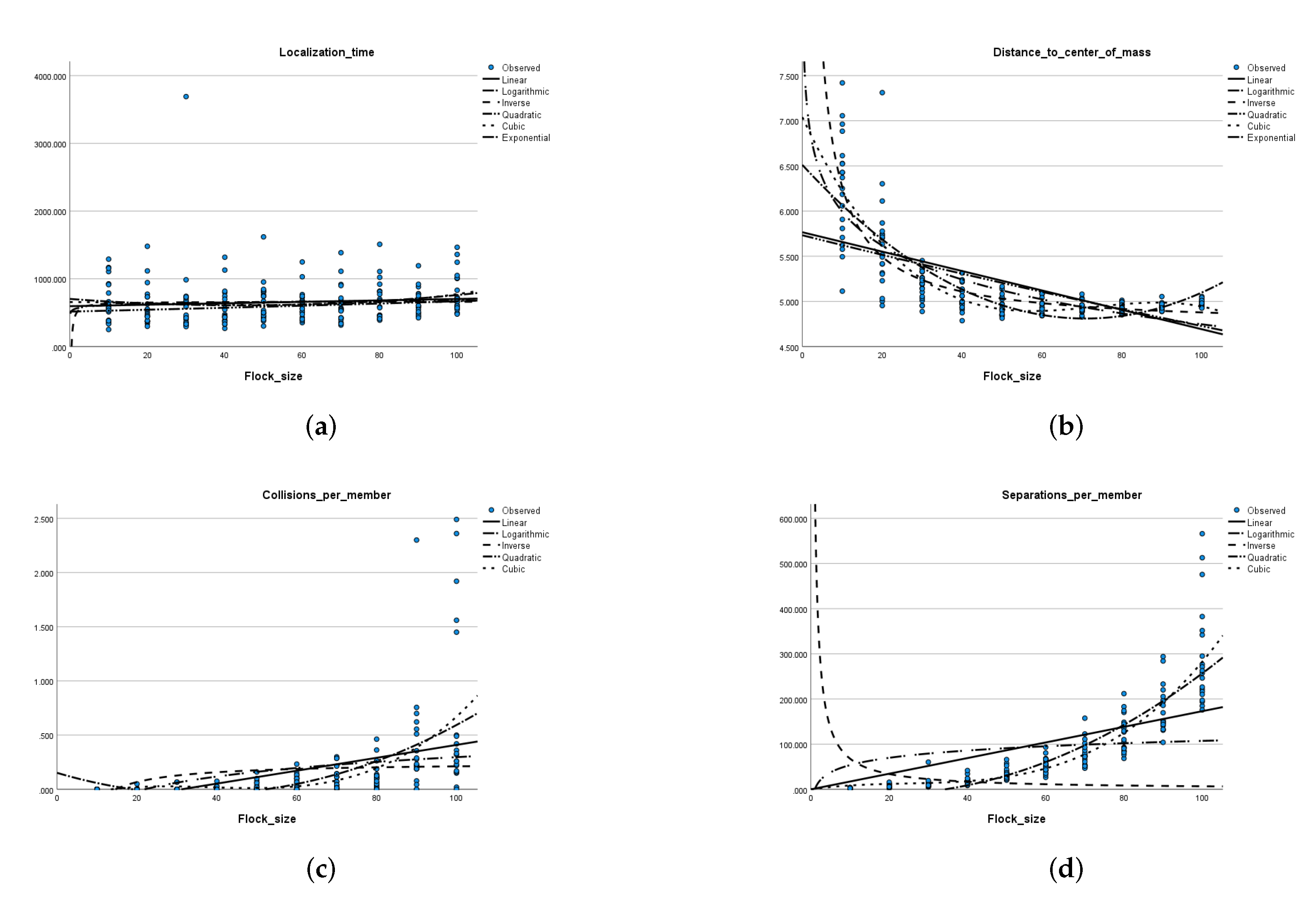
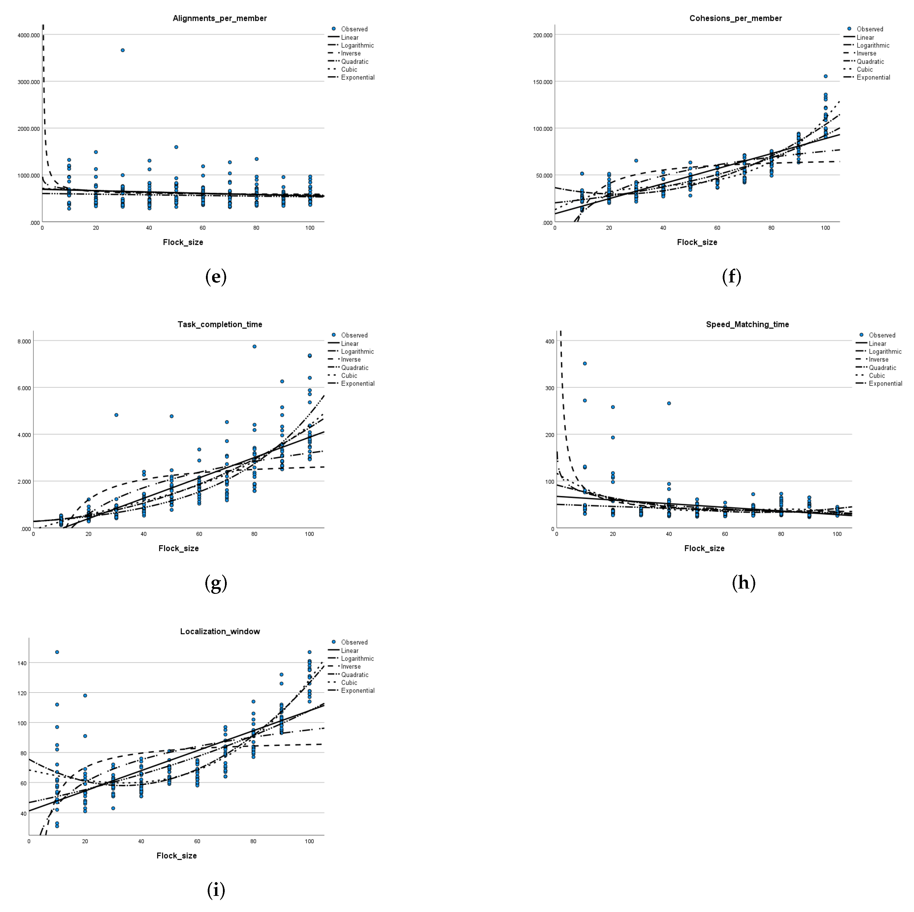
Relationship between the flock size and each of the performance metrics in an environment without obstacles. (a) Flock size versus the goal localization time. (b) Flock size versus the distance to the center of mass. (c) Flock size versus the average number of collisions per member. (d) Flock size versus the average number of applied separation rules per member. (e) Flock size versus the average number of applied alignment rules per member. (f) Flock size versus the average number of applied cohesion rules per member. (g) Flock size versus the average time of task completion. (h) Flock size versus the average speed matching time. (i) Flock size versus the average goal localization window.
Applsci 12 03630 g005aApplsci 12 03630 g005b
Figure 6. 
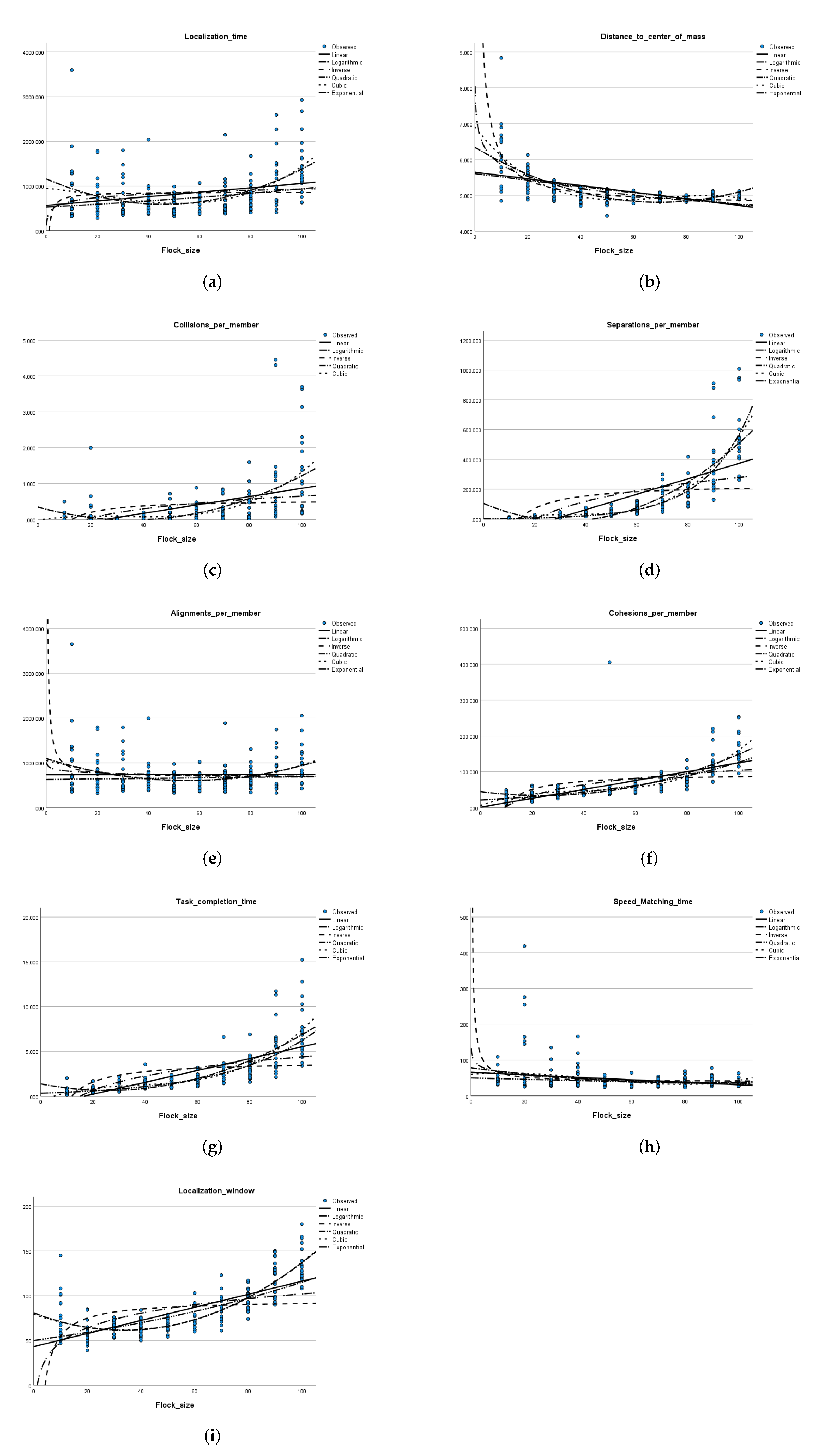
Relationship between the flock size and each of the performance metrics in an environment with obstacles. (a) Flock size versus the goal localization time. (b) Flock size versus the distance to the center of mass. (c) Flock size versus the average number of collisions per member. (d) Flock size versus the average number of applied separation rules per member. (e) Flock size versus the average number of applied alignment rules per member. (f) Flock size versus the average number of applied cohesion rules per member. (g) Flock size versus the average time of task completion. (h) Flock size versus the average speed matching time. (i) Flock size versus the average goal localization window.
Applsci 12 03630 g006
The remainder of this section is organized as follows: Section 3.2.1 reports the results of experiments excluding obstacles. Next, Section 3.2.2 reports the results of experiments including obstacles. All of the experiments used the settings and parameters described in Table 2.

3.2.1. Experimental Results in an Environment without Obstacles

First, we simulated the flocking behavior of 10 100 agents in steps of 10, in an environment without obstacles. In all experiments, the flock completed the flocking task successfully by reaching the goal zone area. Recorded simulation outputs (performance metrics) for each flock size, averaged over twenty runs of each experiment, are shown in Table 3. The relationship is also illustrated in Figure 5. Each sub-figure shows the data results over all experiments for the number of agents (at the x-axis) versus the respective performance metric (at the y-axis) as points distributed on a plane. Moreover, the best-fit curves for each of the nine flocking performance measures against the flock size, using six functions (linear, inverse, logarithmic, quadratic, cubic, and exponential) are shown. The detailed model summary and parameter estimates for the curve fitting obtained are found in Appendix B.
Localization time: Table 3 shows that the average goal zone localization time does not exhibit any monotonic relation along with an increase in the flock size. The distribution of data points in the scatter plot shown in Figure 5a supports this observation. Figure 5a also shows curve estimates for each of the six functions (linear, inverse, logarithmic, quadratic, cubic, and exponential) relating the flock size to the goal localization time. The p-value obtained in each of these models was larger than α = 0.05 (Appendix B); thus, the null hypothesis cannot be rejected, meaning that there exists no association between the changes in flock size and shifts in goal localization time. An exception is the model associated with the exponential function, in which the p-value detected was 0.011 < α ; however, the associated R 2 value indicates that the only 3.2 % of the variation in the localization time is explained by the flock size.
Distance to center of mass: The average distance to center of mass values tend to decrease along with the increase in the flock size (Table 3 and Figure 5b). The flocking behavior is exhibited here, where a larger flock size enables more members to be contained in a flocking zone, allowing the average distance to the center of mass to be reduced. Figure 5b also shows curve estimates for each of the six functions relating the flock size to the distance to center of mass. The p-value obtained for each of these models was less than 0.001 , which means that the sample data provides enough evidence to reject the null hypothesis, and that changes in the flock size are significantly associated with shifts in the distance to center of mass, on the population level. The R 2 value associated with the inverse function for the distance to the center of mass indicates that 69.7 % of the variation in the distance to center of mass is explained by the flock size, while the R 2 value associated with the cube function was somewhat higher than that, at 71.1 % .
Speed matching time: A similar observation of distance to center of mass can be drawn for the speed matching time measure. Figure 5h shows curve estimates for each of the six functions relating the flock size to the speed matching time. The p-value obtained for each of these models was less than 0.001 , which means that the sample data provides enough evidence to reject the null hypothesis, and that changes in the flock size are significantly associated with shifts in the speed matching time on the population level. For the speed matching time, the highest R 2 value is that associated with the inverse function and it accounted for only 12.3 % of the variation in speed matching time due to changes in the flock size.
Collisions per member: The average collisions per member tend to increase along with the increase in the flock size as shown in Table 3. The number of collision avoidance steps needed for a larger flock size is larger than the number needed for a smaller flock size. The scatter plot in Figure 5c also shows that the standard deviation is small (2.5 collisions). The p-value obtained in each of the six curve estimation models was less than 0.001 , which means that the sample data provides enough evidence to reject the null hypothesis, and that changes in the flock size are significantly associated with shifts in the number of collisions on the population level. However, the R 2 values associated with these models are a bit lower than those obtained for the models of the distance to center of mass variable. The R 2 value associated with the quadratic function indicates that 31.5 % of the variation in the number of collisions is explained by the flock size, while the R 2 value associated with the cube function was closely higher than that at 33.7 % .
Separations per member: Table 3 shows a steady increase in the average number of applied separation steps along with the increase in the flock size. The scatter plot in Figure 5d) clearly supports that. The shape of the scatter is close to a quadratic or a cubic function. In fact, the p-value obtained in each of the six curve estimation models was less than 0.001 , which means that the sample data provides enough evidence to reject the null hypothesis, and that changes in flock size are significantly associated with shifts in the number of applied separation steps on the population level. The highest R 2 value is that associated with the cubic function ( 81.4 % ), closely followed by the R 2 value associated with the quadratic function at 79.5 % .
Alignments per member: Similar to goal localization time, Table 3 shows that the average number of alignment steps does not exhibit any monotonic relation along with an increase in the flock size. The distribution of data points in the scatter plot shown in Figure 5e supports this observation. It appears that the average number of alignment steps per member is not affected by the flock size. The scatter of data points appears in every flock size. Figure 5e also shows curve estimates for each of the six functions relating the flock size to the average number of alignment steps per member. The p-value obtained in each of these models was larger than α = 0.05 (Appendix B); thus, the null hypothesis cannot be rejected, meaning that there exists no association between changes in flock size and shifts in the number of alignment steps.
Cohesions per member: The average cohesion steps per member monotonically increases with the increase in the flock size as shown in Table 3, which is confirmed by the scatter plot in Figure 5f. The distribution of data points in the scatter plot shown in Figure 5f shows that the standard deviation of number of cohesion steps is similar for each flock size; however, the average number of cohesion steps increases as the flock size increases. The number of cohesion steps needed to keep a larger flock size in cohesion is larger than the number needed for a smaller flock size. The p-value obtained in each of the six curve estimation models was less than 0.001 , which means that the sample data provides enough evidence to reject the null hypothesis, and that changes in flock size are significantly associated with shifts in the number of cohesion steps on the population level. The highest R 2 value is that associated with the cubic function and explains 87.2 % of the variation in the number of cohesion steps due to shifts in the flock size.
Task completion time and goal localization window: The time required to complete the task in minutes (Figure 5g), as well as the goal localization window (Figure 5i) all increased along with an increase in flock size, as supported by the average value readings from Table 3. The p-value obtained in each of the six curve estimation models for both of these metrics was less than 0.001 , which means that the sample data provides enough evidence to reject the null hypothesis and that changes in flock size are strongly associated with shifts in each of these two performance measures. For the time required to complete the task measure, the highest R 2 value was associated with the exponential function and accounted for 80.2 % of the variation in time required to complete the flocking task due to changes in the flock size. As for the goal localization window, the highest R 2 value was associated with the cubic function and indicates that 75.5 % of the variation in the goal localization window is explained by changes in the flock size, while the R 2 value associated with the quadratic function closely follows at 75.2 % . These results are in line with the shape of the points on the scatter plot in Figure 5i.
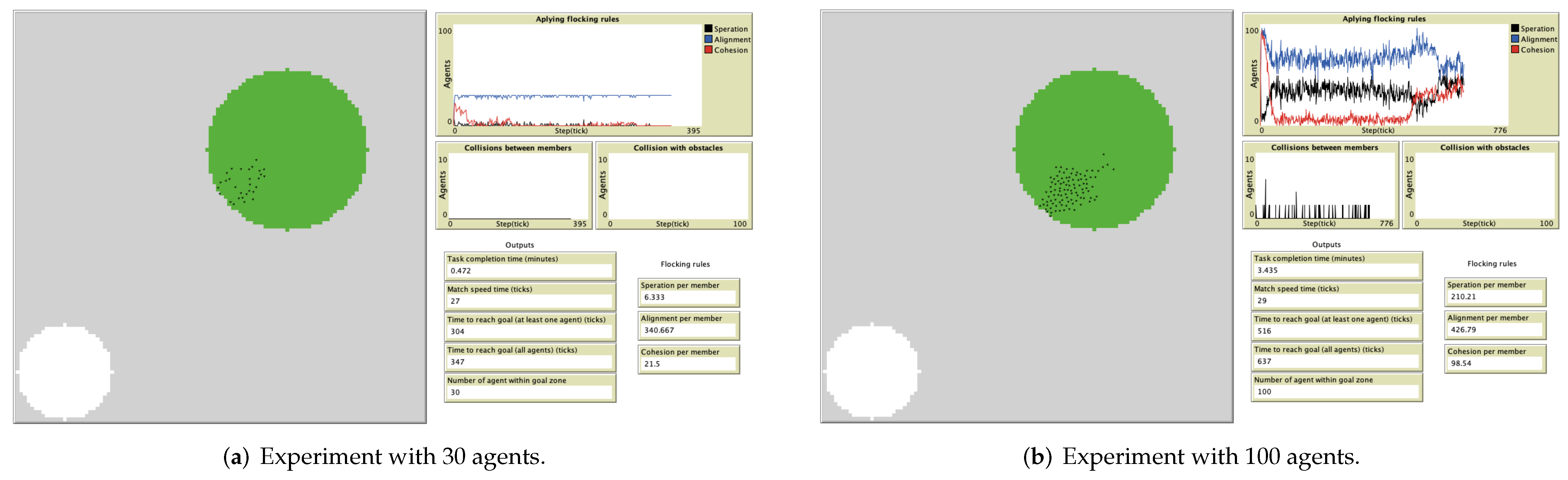
As previously mentioned, the flocking behavior became stable when the majority of the flock members applied the alignment rule, rather than the attraction or separation rules. Based on the obtained results, the larger the flock size, the larger the number of repulsion and cohesion steps applied. The simulation outputs of two randomly selected experiments with flock sizes of 30 and 100 are shown in Appendix C.

3.2.2. Experimental Results in an Environment with Obstacles

Next, experiments simulating the flocking behavior of 10 100 agents in steps of 10, in an environment with obstacles are conducted. In all experiments, the flock was able to complete the flocking task successfully by reaching the goal zone area. Recorded simulation outputs (performance metrics) for each flock size, averaged over twenty runs of each experiment, are shown in Table 4. The relationships are also illustrated in Figure 6. Each sub-figure shows the data results over all experiments for the number of agents (on the x-axis) versus the respective performance metric (on the y-axis) as points distributed on a plane. Moreover, the best-fit curves for each of the nine flocking performance measures against the flock size, using six functions (linear, inverse, logarithmic, quadratic, cubic, and exponential) are shown. The detailed model summary and parameter estimates for the curve fitting obtained are found in Appendix B.
From Table 4 and similar to the observation drawn from results of the experiments without obstacles, no relationship can be easily drawn between the flock size and the goal localization time. The scatter plot in (Figure 6a) shows that the lowest goal localization time was obtained in experiments with 50 agents. Considering the significance of the obtained function curves, interestingly, the p-value associated with each of the different functions was smaller than a l p h a except that for the inverse function. The highest R 2 value was that for the cubic model ( 22.4 % ), closely followed by that for the quadratic model at 21.7 % .
The average distance to center of mass tends to decrease along with an increase in flock size as shown in Table 4. The pattern observed is similar to that illustrated by the results in experiments without obstacles. The p-value associated with all the curve estimation functions in (Figure 6b) supports rejecting the null hypothesis. The R 2 value associated with the inverse function was 57.8 % , while that associated with the cube function was found to be slightly higher at 58.7 % .
Furthermore, similar to the observations drawn from the experiments without obstacles, Table 4 displays a monotonic increase in the average value obtained for each of the performance measures separations, cohesion, and task completion time along with the increase in flock size. The table also shows a tendency of increase in the number of collisions and localization window with the increase in flock size. The p-value obtained for each of the curve estimates in each of (Figure 6c,d,f,g,i) provides strong evidence that the null hypothesis should be rejected. The R 2 value associated with the cubic function in (Figure 6c) was 32.4 % closely followed by that for the quadratic function ( 31.2 % ). Similarly, The R 2 value associated with the cubic function and the quadratic function in (Figure 6i) was, equally, 72.8 % . The highest R 2 value for the models in each of (Figure 6d,f,g) was that associated with the exponential function, having considerable values of 85 % , 70.6 % , and 78.7 % , respectively.
In contrast, considering the number of alignment steps, the p-value obtained for each of the curve estimation values in Figure 6e does not provide sufficient evidence to reject the null hypothesis, except for the cubic and quadratic models. However, the R 2 value associated with these models can only explain the variation in no more than 8.5 % of the number of alignment steps due to the change in flock size.
Finally, the average speed matching time values reported in Table 4 do not show a clear relationship with the flock size. However, the p-value for all the curve estimation functions in Figure 6h for this measure show strong evidence to reject the null hypothesis. Notably, the highest R 2 value obtained from these functions can explain no more than 6.5 % of the change in the speed matching time due to the change in flock size.
The environment had five obstacles, which were added manually to ensure they were distributed along the route to the goal, with random sizes, as illustrated in Figure 7. We applied the same methodology as in the simulation with no obstacles—3 randomly selected experiments of 100, 50, and 30 agents simulation output are shown in Figure 7a–c, respectively. In the upper right corner in these figures, we represent the different flock behaviors: blue curve for number of applied alignment rules, black curve for the number of applied separation rules, and red curve for the number of applied attraction rules. A zoomed-out view of these parameters along with the number of collisions is made clear in Figure 7d. The increase in flock size causes unstable flocking behavior, whereas the flocking rules plot looks smooth in Figure 7a,b. In addition, there is a noticeable increase in the application of the separation and attraction rules (black and red lines, respectively) when the flock size is 100, as shown in Figure 7c. Moreover, whenever the flock does not have stable flocking behavior, the collision between its members increases. In addition, sensing the goal in presence of obstacles close to the goal led to a high possibility that the flock members collide with these obstacles, as shown in Figure 7d.
The flock controller was capable of making the flock split and rejoin to avoid the obstacles, similar to the results reported in [23]. Figure 8 illustrates examples of the splitting (Figure 8a) and joining (Figure 8b) of the flock. This means that the flock was able to split into smaller groups to avoid the obstacle, as long as the obstacle was smaller than the orientation zone’s size.

4. Discussion

The relationship between the flock size and its effect on the flocking system’s performance was analyzed, as measured with respect to several factors, including the flexibility towards reaching the goal (i.e., the time to reach the goal zone, the number of agents within the goal area), the speed matching time, the number of the applied flocking rules (collision avoidance, attraction, and alignment), the localization window, the number of collisions that occurred, the flock’s average distance to the center of mass, and the goal localization time.
Our experiments indicated that the flock was able to reach the goal zone, regardless of the number of agents in the flock; however, the time needed to reach the goal increased as the flock size increased, both in environments with and without obstacles. This was due to the significant increase in applying the rules of separation and cohesion, rather than the rule of alignment. This means that the flock was unable to reach stable flocking behavior properly. Furthermore, as the flock did not possess stable flocking behavior, the chances of collision between its members increased.
Although we did not study the effect of changing the perception zone size as a main factor in this study, it served as a preprocessing step in designing the flock controller. The flocking behavior is highly dependent on the perception zone’s size, as the flocking behavior improves when the orientation zone’s size is large, and the repulsion and attraction zones are small in size. These findings contradict reference [14] in that the zone of attraction is large rather than small; however, the second paper had a smaller flock size, which might affect the results.
Our experiments suggested that flocking behavior becomes more difficult as the flock size increases. This issue is due to the average distance to the center of mass, which becomes smaller with larger flock sizes, as the number of flock members increase in the flocking zone. Moreover, it is related to the size of the perception zone chosen, which may be unsuitable for large-scale flocks. The small average distance to the center of mass indicates that the flock members were close to each other, such that they must keep separating to avoid collisions, in contrast to smaller flock sizes, where the flock members have a high probability of being detected in the orientation zone (alignment with each other), leading to stable flocking behavior. On the other hand, having a larger flock indicates that more agents have a high probability of being detected within the attraction zone (i.e., cohesion with other members), such that the flock members will keep attracting farther members, according to their perception, while avoiding collisions with closer members within the repulsion zone which, in turn, results in unstable flocking behavior.
As the flock size increases, so do the number of collisions, cohesion, and separations. This is expected because of the increase in probability of these events as the number of flock members increases. An increase in the scatter for larger flock sizes can be similarly observed. The increase in flock size creates a more complex environment for the flock to navigate, resulting in a larger variance of flock behavior.
Our findings indicated that the speed matching time slightly decreased along with an increase in the number of agents in an environment without obstacles. On the other hand, the speed matching time was slightly increased in the environments with obstacles. This means that obstacles affect the time to reach the goal, as they hinder exploration. However, the reach time was logically affected by the average speed of the flock. Speed matching time has a larger scatter as the flock size decreases. This is because there are fewer flock members overall within the attraction zone of each flock member, compared with larger flock sizes. The results of reference [14] support our findings, in that each agent’s final desired direction becomes more complicated and takes more time to determine as the size increases.
From our findings we observed that as the flock size increases, the time required to complete the task increases as well, which does not adhere to reference [14]. This discordance is due to the fact that the flock sizes used in their work (with a maximum flock size of 20) were much smaller than the flock sizes used in this work. Moreover, the increase in the time required to complete the task is due to the formation maintenance and cohesion of flock members, which prevents the flock from exploring the environment properly (i.e., presenting stable flocking behavior). Interestingly, the average goal localization time remained unaffected by the flock size, further supporting that an increase in flock size requires higher formation maintenance behavior.
To summarize, flock size does not significantly affect localization time and the number of alignments per flock member. Scatter is homogeneous for all flock sizes. An increase in flock size is positively associated with the number of collisions, separations, and cohesions per flock member. In addition, the localization window and task completion times both increase as flock size increases, and and increase in variability or scatter is seen as well. A decrease in flock size is associated with a larger distance to the center of mass of the flock, as well as larger and more variable speed matching times. Scatter increases with the decrease in flock size.
The results we obtained highlight the critical factors that are affected by changing the flock size, and are expected to be helpful for future research in this field. The limitations of this work lie in the small number of experiments conducted for each flock size due to time constraints. In addition, a sample size of 20 makes it difficult to draw conclusions regarding the apparent outliers in the data, as well as the standard deviation for each flock size. The excessive runtime required for larger flock sizes further prohibits experiments beyond 100 flock members. Furthermore, the controller used in this work may not be fully generalizable to other flocking tasks.

5. Conclusions

In this paper, we studied the impact of changing the flock size on the performance of the flock task. We developed a flock controller using a behavior-based swarm approach and conducted experiments on the problem of reaching a goal zone. Our flock controller depends on the behavior of a flock’s agents, with respect to their neighbors and to the environment. Moreover, the flock controller also introduces the concept of sensing power that replicates the phenomenon observed in nature where migrating birds have a sense of where they need to head, even if they do not precisely know the target. The sensing power provides better take-off results.
In this work, we studied the impact of flock size on flock formation and flock performance through nine different parameters, including the goal zone localization time, the distance to the center of mass, the collisions per member, and the rate of application of the flocking rules. These parameters were measured for ten flocks with increasing size. The flocking behavior was simulated in two different environments, with and without obstacles. The results demonstrated that the developed flock controller is able to deliver the flock to the goal zone, regardless of its size. The experiments concluded that the time required to complete the task in minutes, and the goal localization window increased along with an increase in flock size. The same behavior was observed for the average collisions per member, the average number of applied separations, and the average number of cohesion steps. On the contrary, the results also concluded that the average distance to center of mass, as well as the speed matching time, tend to decrease along with the increase in the flock size. We also observed that the remaining analyzed parameters, namely the goal localization time and the number of applied alignment steps, had no clear association with the variations in the flock size. Overall, similar results were observed in both situations with and without obstacles.
As mentioned above, spatial organization is an area where behavior-based swarm approaches can be applied. This paper studied the impact of the number of agents on the different parameters involved in moving individual robots to spatially organize themselves in a specific region of the environment. As the number of collisions and separations tends to increase with the number of involved agents and certainly impacts the time required to complete the task, in future studies, we intend to work on minimizing the collisions among agents in order to improve the task completion time. We will also study the impact of using the sensing power continuously for motion coordination among the flock and to improve the navigation process. Moreover, the flock controller may integrate other features to memorize discovered areas, which could help reduce the time required to reach the goal.

Author Contributions

Conceptualization, A.T. and R.A.; methodology, S.A. and N.A.; software, R.A.; validation, A.T., R.A., and S.Q.; formal analysis, S.A. and N.A.;writing—original draft preparation, S.A. and R.A.; writing—review and editing, S.A., A.T., S.Q. and N.A.; visualization, R.A.; supervision, A.T.; project administration, S.Q.; funding acquisition, S.Q. All authors have read and agreed to the published version of the manuscript.

Funding

This work was funded by the National Plan for Science, Technology and Innovation (MAARIFAH), King Abdulaziz City for Science and Technology, Kingdom of Saudi Arabia, Award Number (13-SPA1130-02).

Institutional Review Board Statement

Not applicable.

Informed Consent Statement

Not applicable.

Data Availability Statement

Not applicable.

Acknowledgments

The authors would like to thank the anonymous reviewers for their constructive comments. Special thanks to Najla Elhazzani from the Department of Statistics and Operations Research, College of Science, King Saud University for her useful comments.

Conflicts of Interest

The authors declare no conflict of interest. The funders had no role in the design of the study; in the collection, analyses, or interpretation of data; in the writing of the manuscript, or in the decision to publish the results.

Appendix A

This appendix provides details on the tuning of the repulsion orientation and tests for attraction zone radii for flocks with 30, 50, and 100 agents. Table A1 shows the legend used in the results provided in Table A2, Table A3, Table A4. For each used combination of Δ r , Δ o , and Δ a , the obtained objective functions f 1 , f 2 , and f 3 are shown, along with the number of repulsion operations ( r 1 ), the number of alignment operations ( r 2 ), and the number of cohesion operations ( r 3 ) encountered. Combinations of Δ r , Δ o , and Δ a that resulted in unstable flocking behavior for flocks of 30 agents were excluded from experiments considering flocks of 50 agents. Similarly, combinations of Δ r , Δ o , and Δ a that resulted in unstable flocking behavior for flocks of 50 agents were excluded from experiments with flocks of 100 agents.
Table A1. Legend used for Table A2, Table A3, Table A4.
NotationDescription
f 1 localization time of the goal zone
f 2 average distance to the center of mass
f 3 collisions per member
r 1 separation
r 2 alignment
r 3 cohesion
Table A2. Results of testing perception zones for flocks with 30 agents.
Zone RadiiObjective FunctionsFlocking Rules
Δ r Δ o Δ a f 1 f 2 f 3 r 1 r 2 r 3
191 612.90 3.61 0.20 46.97 585.03 43.53
2167.00 3.60 0.00 103.43 2090.57 75.40
953.17 3.58 0.00 59.67 922.33 63.23
1061.27 3.54 0.00 55.00 1031.00 52.20
477.63 3.67 0.07 31.30 468.70 41.57
Average 1054.39 3.60 0.05 59.27 1019.53 55.19
1111 792.67 4.36 0.00 26.00 798.00 51.43
287.80 4.23 0.17 15.67 290.33 22.00
713.20 4.09 0.00 29.03 707.97 28.90
393.80 4.55 0.00 9.03 411.97 29.20
403.93 4.63 0.00 13.40 415.60 38.57
Average 518.28 4.38 0.03 18.63 524.77 34.02
1131 386.90 5.28 0.00 7.90 415.10 25.13
1473.10 5.17 0.00 22.93 1482.07 32.07
369.33 4.82 0.00 7.70 389.30 24.33
563.30 5.05 0.00 9.05 583.5 19.33
419.37 5.29 0.00 12.17 441.83 30.40
Average 642.40 5.12 0.00 12.04 662.36 26.25
168 1785.57 2.62 0.13 587.63 1225.37 243.90
3047.83 2.61 2.27 1150.87 1923.13 423.60
982.50 2.66 1.83 377.07 632.93 185.37
1011.17 2.67 0.00 341.63 701.37 188.27
1465.73 2.69 6.47 609.47 888.53 307.40
Average 1658.56 2.65 2.14 613.33 1074.27 269.707
173 1547.20 2.95 0.43 307.47 1261.53 149.03
3014.27 2.90 1.67 596.73 2434.27 207.97
1339.83 2.96 0.03 183.03 1189.97 123.07
895.03 2.93 2.10 225.40 688.60 107.40
464.50 2.99 0.10 87.33 401.67 73.43
Average 1452.17 2.94 0.87 279.99 1195.21 132.18
164 1873.57 2.61 0.10 633.43 1263.57 233.37
2369.90 2.62 4.53 943.70 1450.30 354.30
3017.73 2.61 4.03 1176.40 1867.60 440.53
1566.63 2.63 4.00 656.90 940.10 269.80
4649.10 2.59 0.03 1551.17 3128.83 521.90
Average 2695.39 2.61 2.54 992.32 1730.08 363.98
172 1815.73 2.94 0.07 291.00 1547.00 141.50
665.00 2.98 0.00 103.40 588.60 76.33
1164.63 2.95 0.83 243.03 942.97 114.37
1656.70 2.95 0.50 311.13 1364.87 132.70
757.87 2.98 0.30 143.37 632.63 78.63
Average 1211.99 2.96 0.34 218.39 1015.21 108.71
Table A3. Results of testing perception zones for flocks with 50 agents.
Zone RadiiObjective FunctionsFlocking Rules
Δ r Δ o Δ a f 1 f 2 f 3 r 1 r 2 r 3
191 700.52 3.64 0.00 173.28 568.72 99.84
588.50 3.72 0.12 148.58 477.42 93.98
1109.44 3.60 0.48 306.78 835.22 114.38
1726.34 3.61 0.16 416.32 1347.68 160.50
601.94 3.67 0.06 164.78 470.22 80.32
Average 945.35 3.65 0.17 241.95 739.85 109.80
1111 1120.60 4.21 0.00 81.86 1073.14 61.46
669.76 4.25 0.26 75.76 623.24 49.36
428.02 4.32 0.02 42.36 418.64 53.30
504.90 4.30 0.01 55.84 481.16 51.94
1617.56 4.19 0.06 199.16 1452.84 83.64
Average 868.17 4.26 0.19 90.99 809.80 59.94
1131 885.46 4.81 0.00 46.98 869.02 41.10
1000.60 4.91 0.32 71.00 963.00 76.90
404.00 4.92 0.00 28.48 410.52 40.90
784.64 4.79 0.52 87.70 726.30 60.28
1121.84 4.84 0.34 88.96 1074.04 75.66
Average 839.31 4.85 0.24 64.62 808.58 58.97
Table A4. Results of testing perception zones for flocks with 100 agents.
Zone RadiiObjective FunctionsFlocking Rules
Δ r Δ o Δ a f 1 f 2 f 3 r 1 r 2 r 3
1131 446.18 5.04 0.98 185.83 326.17 95.23
624.69 4.99 0.58 227.78 455.22 104.96
496.11 5.06 1.15 205.68 353.32 105.11
500.01 4.992 0.28 195.63 368.37 95.67
527.34 4.99 0.46 198.48 383.52 86.95
Average 518.87 5.01 0.69 202.68 377.32 97.58

Appendix B

The detailed model summary and parameter estimates for the curve fitting obtained for each of the nine flocking performance measures, using six functions (linear, inverse, logarithmic, quadratic, cubic, and exponential), where the independent variable is the flock size and the dependent variable is each performance measure, respectively. The model summary and parameter estimates related to experiments without obstacles are provided in Table A5, while Table A6 shows model summary and parameter estimates related to experiments with obstacles. The values b 1 , b 2 , and b 3 represent the regression parameters. For example, a quadratic function will be d e p e n d a n t V a r = c o n s t + ( b 1 × f l o c k S i z e ) + ( b 2 × f l o c k S i z e 2 ) . The p-value significance (Sig.) reflects whether the relationships observed in the data are statistically significant. The standard significance level of α = 0.05 is used. If the p-value < α , then the sample provides enough evidence to reject the null hypothesis; thus, changes in the flock size are associated with changes in the performance measure at the population level. The F-value is related to R 2 and is an indicator of the overall significance through comparing the obtained model against a model that does not contain the flock size (the intercept model). It is used only when the p-value supports rejecting the null hypothesis. The null hypothesis for the F-test states that the model with no flock size fits the data as well as the model provided. The degrees of freedom d f 1 and d f 2 are used to obtain the critical value for the F-test. If the F-value is larger than the critical value, then the associated null hypothesis is rejected, meaning that the data provides enough evidence that the model fits the data better than the intercept-only model. When the dependent variable (performance measure) contains a zero value, the exponential model cannot be calculated for this variable.
Table A5. Model summary and parameter estimates for the curve fitting obtained in experiments without obstacles for each of the nine flocking performance measures, showing five equations (linear, inverse, logarithmic, quadratic, cubic, and exponential), where the independent variable is the flock size and the dependent variable is each performance measure, respectively.
Localization Time
Equation R 2 Model SummaryParameter Estimates
F df 1 df 2 SigConstant b 1 b 2 b 3
Linear0.0081.55111980.21596.801.064
Logarithmic0.0030.62111980.432549.03627.878
Inverse0.0000.09211980.762663.673−284.653
Quadratic0.0181.81921970.165703.633−4.2770.0490.049
Cubic0.0191.25731960.290657.206−0.160−0.0410.001
Exponential0.0326.59511980.011517.0370.003
Distance to Center of Mass
Equation R 2 Model SummaryParameter Estimates
F df 1 df 2 SigConstant b 1 b 2 b 3
Linear0.404134.1271198<0.0015.766−0.011
Logarithmic0.601298.7401198<0.0017.239−0.541
Inverse0.697455.0181198<0.0014.72415.401
Quadratic0.661192.0282197<0.0016.511−0.048<0.000<0.000
Cubic0.711160.5863196<0.0017.040−0.0950.001−6.17 × 10 6
Exponential0.426146.9811198<0.0015.733−0.002
Collisions per Member
Equation R 2 Model SummaryParameter Estimates
F df 1 df 2 SigConstant b 1 b 2 b 3
Linear0.22156.2501198<0.001−0.1850.006
Logarithmic0.14032.2151198<0.001−0.6030.195
Inverse0.06914.6721198<0.0010.248−3.628
Quadratic0.31545.342197<0.0010.152−0.0110.000
Cubic0.33733.2133196<0.001−0.1100.0120.0003.054 × 10 6
Exponential
Separations per Member
Equation R 2 Model SummaryParameter Estimates
F df 1 df 2 SigConstant b 1 b 2 b 3
Linear0.650368.1841198<0.001−71.9422.758
Logarithmic0.452163.1341198<0.001−282.28494.948
Inverse0.24664.7621198<0.001134.062−1854.17
Quadratic0.795382.7652197<0.00141.334−2.9060.051
Cubic0.814286.5733196<0.001−24.7982.960−0.0760.001
Exponential
Alignments per Member
Equation R 2 Model SummaryParameter Estimates
F df 1 df 2 SigConstant b 1 b 2 b 3
Linear0.0153.00111970.085692.039−1.389
Logarithmic0.0152.95411970.087832.665−56.934
Inverse0.0132.50711970.115574.8671388.522
Quadratic0.0151.49821960.226699.440−1.7600.003
Cubic0.0150.99931950.394713.458−3.0030.0300.00
Exponential0.0081.66011970.199604.031−0.001
Cohesions per Member
Equation R 2 Model SummaryParameter Estimates
F df 1 df 2 SigConstant b 1 b 2 b 3
Linear0.725521.9411198<0.00018.6250.802
Logarithmic0.536228.3701198<0.001−55.87128.490
Inverse0.32294.0271198<0.00169.866−583.987
Quadratic0.840517.2442197<0.00136.426−0.5880.013
Cubic0.872443.7663196<0.00112.9191.497−0.0330.000
Exponential0.782710.3181198<0.00120.2780.015
Task Completion Time
Equation R 2 Model SummaryParameter Estimates
F df 1 df 2 SigConstant b 1 b 2 b 3
Linear0.649365.9441198<0.001−0.4660.043
Logarithmic0.527220.2531198<0.001−4.2381.615
Inverse0.340102.1411198<0.0012.928−34.333
Quadratic0.674203.9702197<0.0010.2820.0060.000
Cubic0.677136.6923196<0.001−0.0770.0380.0004.19 × 10 6
Exponential0.802801.1401198<0.0010.2750.029
Speed Matching Time
Equation R 2 Model SummaryParameter Estimates
F df 1 df 2 SigConstant b 1 b 2 b 3
Linear0.07616.1901198<0.00167.367−0.390
Logarithmic0.10924.1921198<0.001119.687−19.353
Inverse0.12327.7031198<0.00129.984543.230
Quadratic0.11412.7162197<0.00191.675−1.6060.011
Cubic0.1309.7483196<0.001116.462−3.8040.0590.000
Exponential0.07816.7421198<0.00150.279−0.005
Localization Window
Equation R 2 Model SummaryParameter Estimates
F df 1 df 2 SigConstant b 1 b 2 b 3
Linear0.558249.6271198<0.00141.2700.667
Logarithmic0.347105.0291198<0.001−4.83521.707
Inverse0.15436.0521198<0.00189.141−382.579
Quadratic0.752298.5782197<0.00175.487−1.0440.016
Cubic0.755201.5543196<0.00168.335−0.4100.0028.34 × 10 5
Exponential0.591286.4851198<0.00146.8420.008
Table A6. Model summary and parameter estimates for the curve fitting obtained in experiments with obstacles for each of the nine flocking performance measures, showing five equations (linear, inverse, logarithmic, quadratic, cubic, and exponential) where the independent variable is the flock size and the dependent variable is each performance measure, respectively.
Localization Time
Equation R 2 Model SummaryParameter Estimates
F df 1 df 2 SigConstant b 1 b 2 b 3
Linear0.07415.811198<0.001567.8764.90
Logarithmic0.0255.12611980.025386.60118.218
Inverse0.0030.52611980.469867.027−1012.61
Quadratic0.21727.3292197<0.0011160.904−24.7520.270
Cubic0.22418.873196<0.001950.885−6.124−0.1340.002
Exponential0.10423.0301198<0.001529.6310.006
Distance to Center of Mass
Equation R 2 Model SummaryParameter Estimates
F df 1 df 2 SigConstant b 1 b 2 b 3
Linear0.30586.7801198<0.0015.647−0.009
Logarithmic0.476179.5591198<0.0016.967−0.481
Inverse0.578271.3021198<0.0014.72414.011
Quadratic0.529110.6452197<0.0016.342−0.0440.000
Cubic0.58792.8243196<0.0016.911−0.0950.001−6.64 × 10 6
Exponential0.33298.2791198<0.0015.605−0.002
Collisions per Member
Equation R 2 Model SummaryParameter Estimates
F df 1 df 2 SigConstant b 1 b 2 b 3
Linear0.22356.7371198<0.001−0.2960.012
Logarithmic0.14132.5701198<0.001−1.1170.384
Inverse0.07115.0291198<0.0010.555−7.166
Quadratic0.31244.7592197<0.0010.348−0.0210.000
Cubic0.32431.2933196<0.001−0.0230.0120.0004.32 × 10 6
Exponential
Separations per Member
Equation R 2 Model SummaryParameter Estimates
F df 1 df 2 SigConstant b 1 b 2 b 3
Linear0.536228.3561198<0.001−144.4105.184
Logarithmic0.357109.9641198<0.001−525.907174.826
Inverse0.18745.5611198<0.001238.693−3345.39
Quadratic0.700229.4662197<0.001105.097−7.2910.113
Cubic0.728174.6523196<0.001−61.3957.476−0.2070.002
Exponential0.8501124.1721198<0.0012.3640.055
Alignments per Member
Equation R 2 Model SummaryParameter Estimates
F df 1 df 2 SigConstant b 1 b 2 b 3
Linear0.0000.00411980.952734.9740.062
Logarithmic0.0061.17411980.280912.056−45.548
Inverse0.0193.78411980.053675.4812147.55
Quadratic0.0849.0362197<0.0011096.958−18.0370.165
Cubic0.0856.0313196<0.0011052.835−14.1240.0800.001
Exponential0.0040.77211980.381627.1650.001
Cohesions per Member
Equation R 2 Model SummaryParameter Estimates
F df 1 df 2 SigConstant b 1 b 2 b 3
Linear0.478181.2151198<0.0010.8721.242
Logarithmic0.351107.2151198<0.001−98.54743.993
Inverse0.20852.0581198<0.00195.423−895.367
Quadratic0.556123.5822197<0.00144.686−0.9480.020
Cubic0.58190.5093196<0.0015.4022.536−0.0560.000
Exponential0.706474.8531198<0.00121.1050.018
Task Completion Time
Equation R 2 Model SummaryParameter Estimates
F df 1 df 2 SigConstant b 1 b 2 b 3
Linear0.559250.8171198<0.001−1.0990.066
Logarithmic0.403133.7671198<0.001−6.3192.325
Inverse0.23460.3361198<0.0013.916−46.781
Quadratic0.662192.7462197<0.0011.375−0.0570.001
Cubic0.684141.3513196<0.001−0.4730.106−0.0022.15 × 10 5
Exponential0.787730.1941198<0.0010.3330.029
Speed Matching Time
Equation R 2 Model SummaryParameter Estimates
F df 1 df 2 SigConstant b 1 b 2 b 3
Linear0.05712.0771198<0.00165.663−0.349
Logarithmic0.05511.5971198<0.001100.397−14.144
Inverse0.0316.30911980.01338.283279.349
Quadratic0.0687.13121970.00178.338−0.9830.006
Cubic0.0765.34631960.00159.9400.649−0.0300.000
Exponential0.06513.7921198<0.00149.904−0.004
Localization Window
Equation R 2 Model SummaryParameter Estimates
F df 1 df 2 SigConstant b 1 b 2 b 3
Linear0.538230.7211198<0.00143.1730.730
Logarithmic0.32996.8631198<0.001−6.52823.570
Inverse0.13831.8071198<0.00195.192−404.476
Quadratic0.728263.9162197<0.00180.919−1.1570.017
Cubic0.728175.1653196<0.00179.337−1.0170.0141.84 × 10 5
Exponential0.570262.1201198<0.00150.0490.008

Appendix C

The simulation outputs of two randomly selected experiments with flock sizes of 30 and 100 are shown in Figure A1a and Figure A1b, respectively. In the upper right corner in these figures, we represent the different flock behaviors: blue curve for number of applied alignment rules, black curve for the number of applied separation rules, and red curve for the number of applied attraction rules. Increases in the flock size caused unstable flocking behavior, as the application of the flocking rules shows, where the blue line looks smooth in Figure A1a. There was also a noticeable increase with the application of the separation and attraction rules (black and red lines, respectively) when the flock size was 100, as shown in Figure A1b.
Figure A1. Snapshots of simulation experiments with flock sizes of 30 and 100, in an environment without obstacles.
Applsci 12 03630 g0a1

References

  1. Dang, A.D.; La, H.M.; Nguyen, T.; Horn, J. Distributed Formation Control for Autonomous Robots in Dynamic Environments. arXiv 2017, arXiv:1705.02017. [Google Scholar]
  2. Zhu, P.; Dai, W.; Yao, W.; Ma, J.; Zeng, Z.; Lu, H. Multi-robot flocking control based on deep reinforcement learning. IEEE Access 2020, 8, 150397–150406. [Google Scholar]
  3. Janson, S.; Merkle, D.; Middendorf, M. A decentralization approach for swarm intelligence algorithms in networks applied to multi swarm PSO. Int. J. Intell. Comput. Cybern. 2008, 1, 25–45. [Google Scholar] [CrossRef]
  4. Liu, Y.; Bucknall, R. A survey of formation control and motion planning of multiple unmanned vehicles. Robotica 2018, 36, 1019–1047. [Google Scholar]
  5. Cheraghi, A.R.; Ben Janete, A.; Graffi, K. Robot Swarm Flocking on a 2D Triangular Graph. In Proceedings of the 2020 5th Asia-Pacific Conference on Intelligent Robot Systems (ACIRS), Singapore, 17–19 July 2020; pp. 154–162. [Google Scholar] [CrossRef]
  6. Brambilla, M.; Ferrante, E.; Birattari, M.; Dorigo, M. Swarm robotics: A review from the swarm engineering perspective. Swarm Intell. 2013, 7, 1–41. [Google Scholar] [CrossRef] [Green Version]
  7. Schranz, M.; Umlauft, M.; Sende, M.; Elmenreich, W. Swarm Robotic Behaviors and Current Applications. Front. Robot. AI 2020, 7, 36. [Google Scholar] [CrossRef] [Green Version]
  8. Dias, P.G.F.; Silva, M.C.; Filho, G.P.R.; Vargas, P.A.; Cota, L.P.; Pessin, G. Swarm Robotics: A Perspective on the Latest Reviewed Concepts and Applications. Sensors 2021, 21, 2062. [Google Scholar] [CrossRef]
  9. Hamann, H. Swarm Robotics: A Formal Approach; Springer: Berlin/Heidelberg, Germany, 2018. [Google Scholar]
  10. Hamann, H; Schmickl, T; Modelling the swarm: Analysing biological and engineered swarm systems. Math. Comput. Model. Dyn. Syst. 2012, 18, 1–12. [CrossRef]
  11. Reynolds, C.W. Flocks, herds and schools: A distributed behavioral model. In Proceedings of the 14th Annual Conference on Computer Graphics and Interactive Techniques, Anaheim, CA, USA, 27–31 July 1987; pp. 25–34. [Google Scholar]
  12. Zheng, H.; Panerati, J.; Beltrame, G.; Prorok, A. An adversarial approach to private flocking in mobile robot teams. IEEE Robot. Autom. Lett. 2020, 5, 1009–1016. [Google Scholar]
  13. Couzin, I.D.; Krause, J.; James, R.; Ruxton, G.D.; Franks, N.R. Collective memory and spatial sorting in animal groups. J. Theor. Biol. 2002, 218, 1–11. [Google Scholar]
  14. Márquez-Vega, L.A.; Aguilera-Ruiz, M.; Torres-Treviño, L.M. Multi-objective optimization of a quadrotor flock performing target zone search. Swarm Evol. Comput. 2021, 60, 100733. [Google Scholar]
  15. Oh, K.K.; Park, M.C.; Ahn, H.S. A survey of multi-agent formation control. Automatica 2015, 53, 424–440. [Google Scholar]
  16. Yu, J.; Ji, J.; Miao, Z.; Zhou, J. Region-based flocking control for networked robotic systems with communication delays. Eur. J. Control. 2020, 52, 78–86. [Google Scholar]
  17. Ávila-Martínez, E.J.; Barajas-Ramírez, J.G. Flocking motion in swarms with limited sensing radius and heterogeneous input constraints. J. Frankl. Inst. 2021, 358, 2346–2366. [Google Scholar]
  18. Etemadi, S.; Vatankhah, R.; Alasty, A.; Vossoughi, G.R.; Boroushaki, M. Leader connectivity management and flocking velocity optimization using the particle swarm optimization method. Sci. Iran. 2012, 19, 1251–1257. [Google Scholar]
  19. Wei, H.; Chen, X.B. Flocking for multiple subgroups of multi-agents with different social distancing. IEEE Access 2020, 8, 164705–164716. [Google Scholar]
  20. Kahn, A.; Marzat, J.; Piet-Lahanier, H. Formation flying control via elliptical virtual structure. In Proceedings of the 2013 10th IEEE International Conference on Networking, Sensing and Control (ICNSC), Evry, France, 10–12 April 2013; pp. 158–163. [Google Scholar]
  21. Liu, H.; Wang, X.; Liu, Y.; Li, X. On non-collision flocking and line-shaped spatial configuration for a modified singular Cucker–Smale model. Commun. Nonlinear Sci. Numer. Simul. 2019, 75, 280–301. [Google Scholar]
  22. Cao, Y.U.; Kahng, A.B.; Fukunaga, A.S. Cooperative mobile robotics: Antecedents and directions. In Robot Colonies; Springer: Berlin/Heidelberg, Germany, 1997; pp. 7–27. [Google Scholar]
  23. Olfati-Saber, R. Flocking for multi-agent dynamic systems: Algorithms and theory. IEEE Trans. Autom. Control 2006, 51, 401–420. [Google Scholar]
  24. Semnani, S.H.; Basir, O.A. Semi-flocking algorithm for motion control of mobile sensors in large-scale surveillance systems. IEEE Trans. Cybern. 2014, 45, 129–137. [Google Scholar]
  25. Khrustalev, M.M. Synthesis of adaptive control strategies for flocks of mobile robots using Aristotle’s mechanics. IFAC-PapersOnLine 2018, 51, 525–529. [Google Scholar]
  26. Zhang, H.; Nie, P.; Sun, Y.; Shi, Y. Fixed-time flocking problem of a Cucker–Smale type self-propelled particle model. J. Frankl. Inst. 2020, 357, 7054–7068. [Google Scholar]
  27. Krause, J.; Ruxton, G.D.; Ruxton, G.; Ruxton, I.G. Living in Groups; Oxford University Press: New York, NY, USA, 2002. [Google Scholar]
  28. Caro, T. Antipredator Defenses in Birds and Mammals; University of Chicago Press: Chicago, IL, USA, 2005. [Google Scholar]
  29. McSweeney, P.L.; McNamara, J.P. Encyclopedia of Dairy Sciences, 3rd ed.; Academic Press: Cambridge, MA, USA, 2021. [Google Scholar]
  30. Cresswell, W.; Quinn, J.L. Predicting the optimal prey group size from predator hunting behaviour. J. Anim. Ecol. 2011, 80, 310–319. [Google Scholar]
  31. Vine, I. Detection of prey flocks by predators. J. Theor. Biol. 1973, 40, 207–210. [Google Scholar]
  32. Hintz, W.D.; Lonzarich, D.G. Maximizing foraging success: The roles of group size, predation risk, competition, and ontogeny. Ecosphere 2018, 9, 10. [Google Scholar]
  33. Rakić, K.; Rosić, M.; Boljat, I. A Survey of Agent-Based Modelling and Simulation Tools for Educational Purpose. Tehnički Vjesnik 2020, 27, 1014–1020. [Google Scholar]
  34. Abar, S.; Theodoropoulos, G.K.; Lemarinier, P.; O’Hare, G.M. Agent Based Modelling and Simulation tools: A review of the state-of-art software. Comput. Sci. Rev. 2017, 24, 13–33. [Google Scholar]
  35. Tisue, S.; Wilensky, U. NetLogo: Design and implementation of a multi-agent modeling environment. In Proceedings of Agent; Springer: Cham, Switzerland, 2004; Volume 2004, pp. 7–9. [Google Scholar]
  36. Pallant, J. SPSS Survival Manual: A Step by Step Guide to Data Analysis Using IBM SPSS; Routledge: Oxfordshire, UK, 2020. [Google Scholar]
  37. Johnson, R.A.; Wichern, D.W. Applied Multivariate Statistical Analysis; Pearson: London, UK, 2014; Volume 6. [Google Scholar]
  38. Cohen, J. Statistical Power Analysis for the Behavioral Sciences; Routledge: Oxfordshire, UK, 2013. [Google Scholar]
  39. Guest, P.G. Numerical Methods of Curve Fitting; Cambridge University Press: Cambridge, NY, USA, 2012. [Google Scholar]
  40. Smith, K.; Fry, P.; Shannon, P.; Groebner, D. Business Statistics: A Decision-making Approach. J.-Oper. Res. Soc. 2005, 56, 1347. [Google Scholar]
Figure 1. Sensing zones and view sectors of agents: (a) The three agent perception zones; and (b) the eight view sectors.
Applsci 12 03630 g001
Figure 2. Sensing power and its field of attraction.
Applsci 12 03630 g002
Figure 3. Arena specifications, including ratios.
Applsci 12 03630 g003
Figure 4. Arena specifications ratio. The circle on the left displays an enlarged patch.
Applsci 12 03630 g004
Figure 7. Snapshots of simulation experiments with flock sizes of 30, 50, and 100, in an environment with obstacles. (a) Experiment 1 with 30 agents. (b) Experiment with 50 agents. (c) Experiment with 100 agents. (d) Focus on the flocking rules and number of collisions for experiment with 100 agents. (Figure 7c).
Applsci 12 03630 g007
Figure 8. Illustration of flock splitting and rejoining. (a) Flock splitting. (b) Flock rejoin.
Applsci 12 03630 g008
Table 1. Notation used for the design of the flock controller.
NotationDefinition
nNumber of agents
TTotal number of steps
g i The status of goal detection of agent i
s e p s The total number of applied separations at step s
a l s The total number of applied alignments at step s
c o s The total number of applied cohesions at step s
s i The i th agent’s total steps for the localization of the goal zone
c s The average center of mass of the flock at a specific step s
r i , s The i th agent’s linear position at step s
d ( c s , r i , s ) The Euclidean distance between points c s , and r i , s
D s A matrix with the Euclidean distance between each pair of agents i and j at step s (Equation (14))
a s The number of collisions between agents at step s (Equation (15))
d c The maximum collision distance between agents
o i Obstacles detected by agent i (Equation (16))
o s A vector of of all o i , i n agents at step s (Equation (17))
b s The total number of collisions at step s (Equation (18))
Table 2. Simulation parameter values.
ParameterValue
n 10 100 agents in steps of 10
Arena size 112 × 112 m
Initiate zone radius13 m
Goal zone radius22 m
Patch size 5.5 × 5.5 pixels, corresponding to 1 m 2
d c 0.55 patch
step1 s
Agent speedRandom number ∈[0–0.5] Patch
Δ r 1 patch
Δ o 13 patch
Δ a 1 patch
Priority weights w 1 = 0.4 , w 2 = 0.075 , w 3 = 0.025
Table 3. Performance metric results averaged over twenty simulations for flock sizes in 10 100 , in an environment without obstacles.
Flock Size
Performance Metric1020304050
Localization Time673.20594.96673.19564.29661.26
Distance to center of mass6.255.635.175.034.96
Collisions0.000.000.010.010.03
Separations1.856.9812.5818.4634.80
Alignments706.40616.23690.57580.90668.76
Cohesions25.2232.8534.4135.8342.83
Task completion time0.300.510.881.061.65
Speed matching time82.3068.633.0054.8534.50
Localization window66.4558.6558.6560.6066.75
Flock Size
Performance Metric60708090100
Localization Time627.81615.74688.05654.63800.21
Distance to center of mass4.944.934.924.954.98
Collisions0.070.100.120.400.68
Separations53.5577.70122.61175.68293.34
Alignments606.85578.00609.39530.52571.07
Cohesions46.3353.0663.7080.56112.82
Task completion time1.812.162.913.564.38
Speed matching time30.7538.2543.8039.9033.00
Localization window66.0078.3089.45104.15130.35
Table 4. Performance metric results averaged over twenty simulations for flock sizes in 10 100 , in an environment with obstacles.
Flock Size
Performance Metric1020304050
Localization Time900.14749.98715.60685.07590.01
Distance to center of mass6.155.465.154.954.94
Collisions0.040.180.010.030.13
Separations3.2411.0919.2933.4644.22
Alignments934.81767.37729.91684.20580.33
Cohesions28.6433.5742.1542.3963.13
Task completion time0.450.741.011.421.47
Speed matching time48.0595.444.2557.836.00
Localization window73.2558.164.965.266.5
Flock Size
Performance Metric60708090100
Localization Time634.24743.43787.131126.951441.14
Distance to center of mass4.944.924.924.974.96
Collisions0.200.270.360.931.31
Separations74.50126.63168.83364.80561.03
Alignments595.10658.57665.22821.15947.17
Cohesions55.2466.4876.03125.26159.10
Task completion time1.912.533.205.347.39
Speed matching time30.4533.4539.5039.5034.20
Localization window71.583.5594.7119.85135.9
Publisher’s Note: MDPI stays neutral with regard to jurisdictional claims in published maps and institutional affiliations.

