Time-Varying Topology Formation Reconfiguration Control of the Multi-Agent System Based on the Improved Hungarian Algorithm

Abstract

Distributed time-varying formation technology for multi-agent systems is recently become a research hotspot in formation control field. However, the formation reconfiguration control technology for agents that randomly appeared to fail during maneuvers is rarely studied. In this paper, the topological relations between intelligence are designed by graph theory to simplify the cooperative interaction between multi-agent systems. Moreover, this paper constructs the time-varying configuration of the target formation based on the rigidity graph theory and leader–follower strategy. Drawing on the establishment of the expert experience database in a collaborative process, we innovatively propose the establishment of a graphic library to help the multi-agent system quickly form an affine transformation as soon as it is disabled. Secondly, the improved Hungarian algorithm is adopted to allocate the target point when the first failure occurs. This algorithm incorporates a gradient weighting factor from the auction algorithm to improve the speed of system reconfiguration with minimum path cost. On this basis, a distributed multi-agent control law based on consistency theory is established, and the system’s stability can be guaranteed via Lyapunov functions. Finally, the simulation results demonstrate the feasibility and effectiveness of the proposed formation reconfiguration control algorithm in a collaborative environment.

1. Introduction

The multi-agent system has replaced human beings to perform specific complex tasks and has achieved remarkable results in intelligent scenarios. Multi-agent cooperation will have a higher value in the future and have excellent developmental prospects [1,2]. Facing complex environments, the multi-agent system needs to deal with agent disability, communication disconnection, and other emergencies to ensure the overall survivability of the system [3]. Therefore, achieving the formation, reconstruction, and transformation of multi-agent formations under time-varying topology is one of the difficulties in the collaborative control of multi-agent systems [4].

Nowadays, there is a large amount of theoretical and practical research on the formation and reconstruction technology of multi-agent clusters [5,6]. In Ref. [7], the leader-follower method is adopted to realize multi-robot formation control, and the follower layer is controlled according to the information of the leader layer. This method depends on the state of the leader and has poor robustness [8]. Ref. [9] combines the artificial potential field with the virtual structure. The potential field repulsion function is used to realize collision avoidance and the virtual structure can be tracked to form the AUV formation. The artificial potential field method easily falls into the local minimum point, and it is difficult to reach the global optimal. In Ref. [10], the concept of escape angle is introduced to determine the heading angle of the robot, and the behavior-based method is adopted to implement obstacle-avoiding formation control. The behavior of this method in dynamic and complex environments is unpredictable and needs better flexibility. The above documents use different control strategies to solve the formation control of multi-agent systems but do not consider the possible reconstruction problems in the formation process.

Numerous studies have been conducted to address issues such as the UAV formation and reconfiguration. In Ref. [11], a sliding mode method is used to design a time-varying formation output tracking controller to deal with uncertainties and external disturbances. In Ref. [12], a new speed and lateral channel controller was designed to limit the deviation during formation transformation, so as to improve the rapidity and stability of reconfiguration. However, most of the papers focus on time-varying formations and reconfigurations for uncertainties in dynamic models, practical constraints and external disturbances, and the formation topology is generally fixed.

In complex environments such as blocked communications, the execution of tasks via multi-agent systems is affected by many factors, and the failure of a single agent is a typical situation. If a fixed topology is adopted, multi-agent systems cannot cooperate to complete subsequent tasks when confronted with an unexpected situation. Switching communication topology can effectively solve the multi-agent system configuration reconstruction. In Ref. [13], the multi-agent network topology is switched according to the Markov random transition and the mean square consistency problem of the Lure-type multi-agent system with time delay and topology uncertainty is considered. The virtual leader is designed to assign the trajectory of systems in Ref. [14]. Subgroups can interact with each other by cooperation among group leaders such that the relative configuration between different groups can be adjusted simultaneously. In Ref. [15], the leader’s control input is unknown, and the followers are prone to being influenced. The algorithms apply the idea of simply disregarding a certain number of extreme values to rule against the misbehaviors of affected agents. However, the article mentioned above do not consider the energy consumption of formation reconstruction of multi-agent systems after switching topology.

The complex task requirements of multi-agent systems involve switching between different formation configurations. Energy waste may occur if the system switches from Formation A to Formation B without position reassignment. For multi-agent systems with a limited load capacity, saving energy in the process of collaboration is particularly important. As a consequence, this paper applies the switching communication topology to the process of formation reconfiguration and adds the improved Hungarian algorithm for the distribution of reconfiguration target points. The method takes the total distance of the system as the shortest to obtain the optimal performance and improve the efficiency of cluster reconstruction and collaborative task execution. On this basis, a multi-agent distributed formation control strategy based on the double integrator model is proposed, and the convergence and stability of the system are discussed. Finally, the formation reconstruction of the time-varying topology is realized through simulation, which verifies the feasibility of the reconstruction strategy designed in this paper.

The contribution of this paper can be summarized as follows:

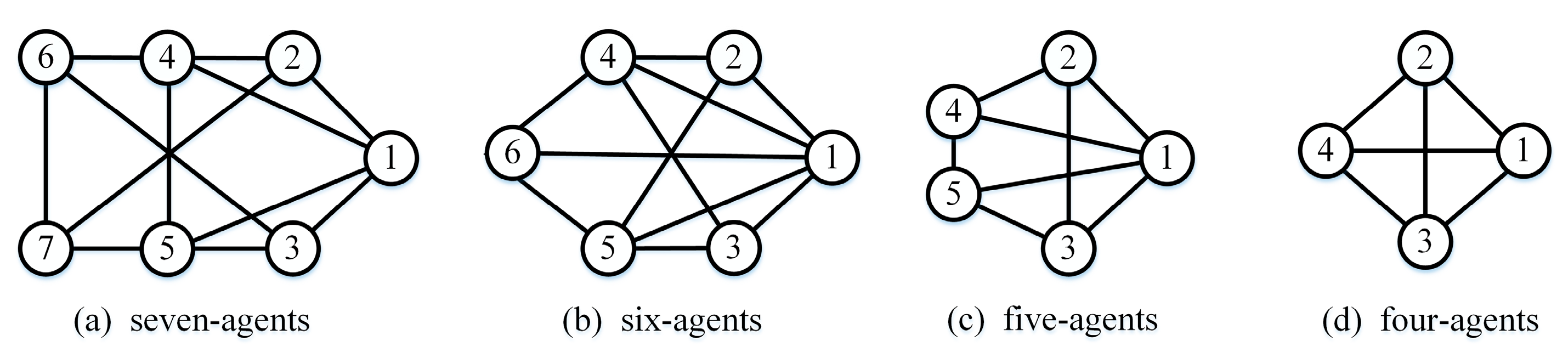
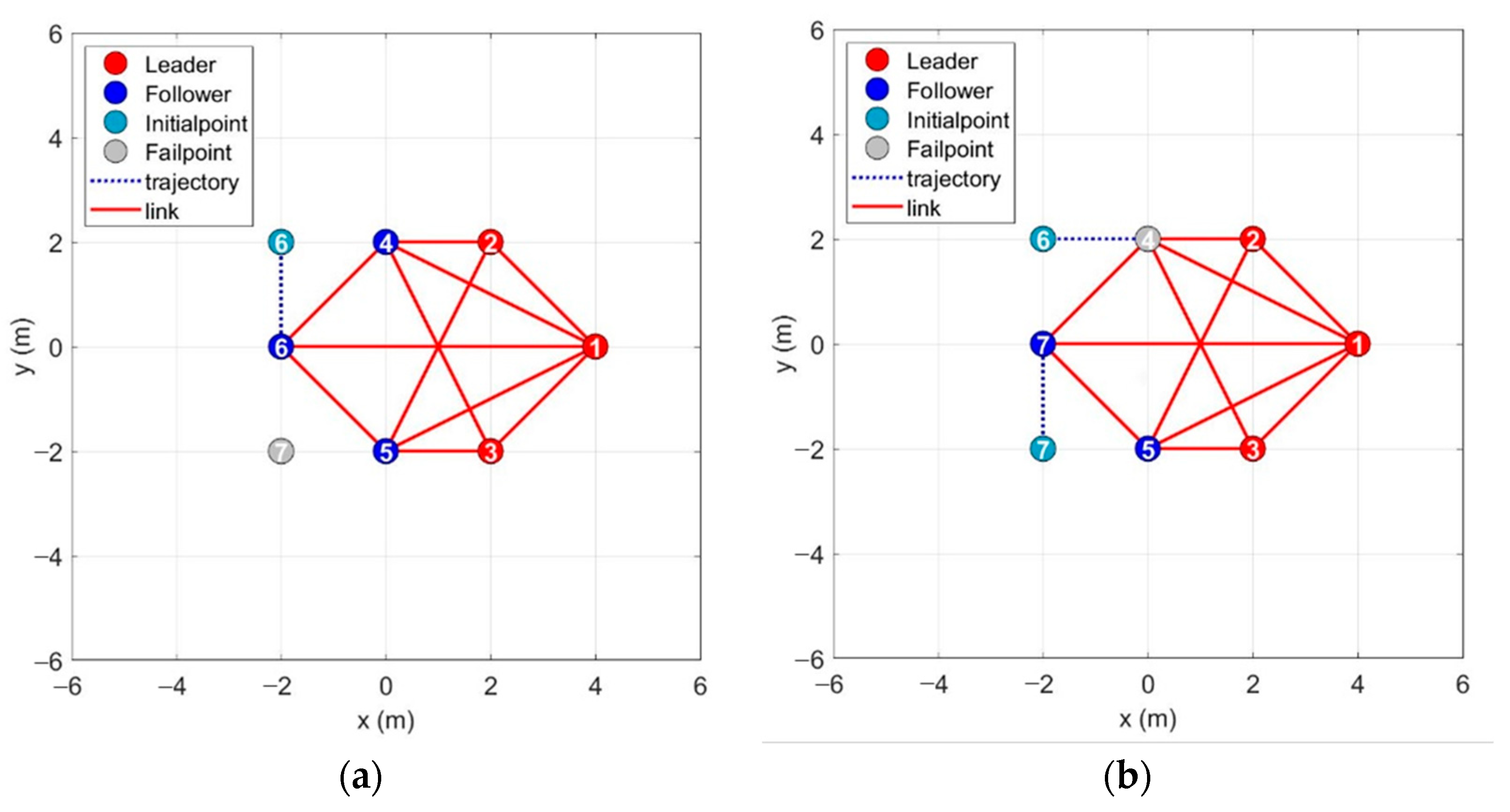
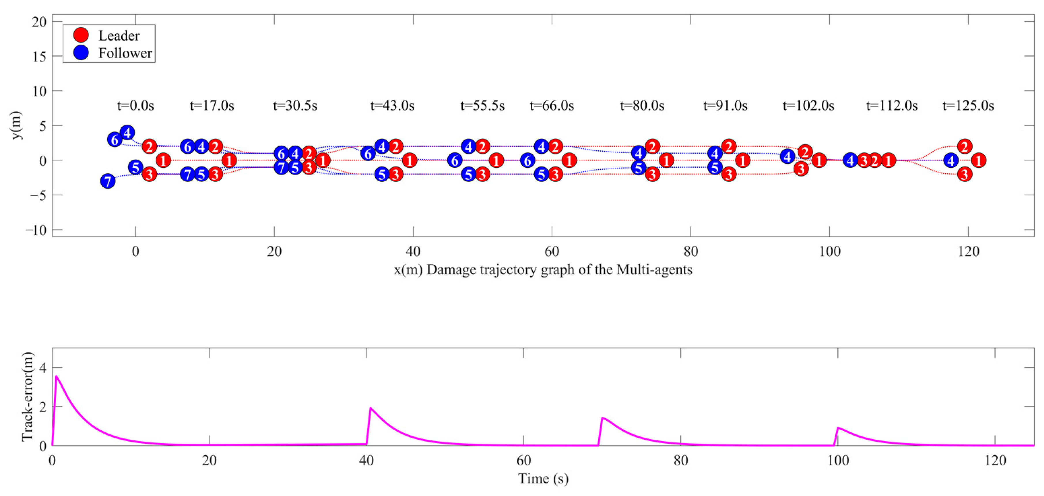
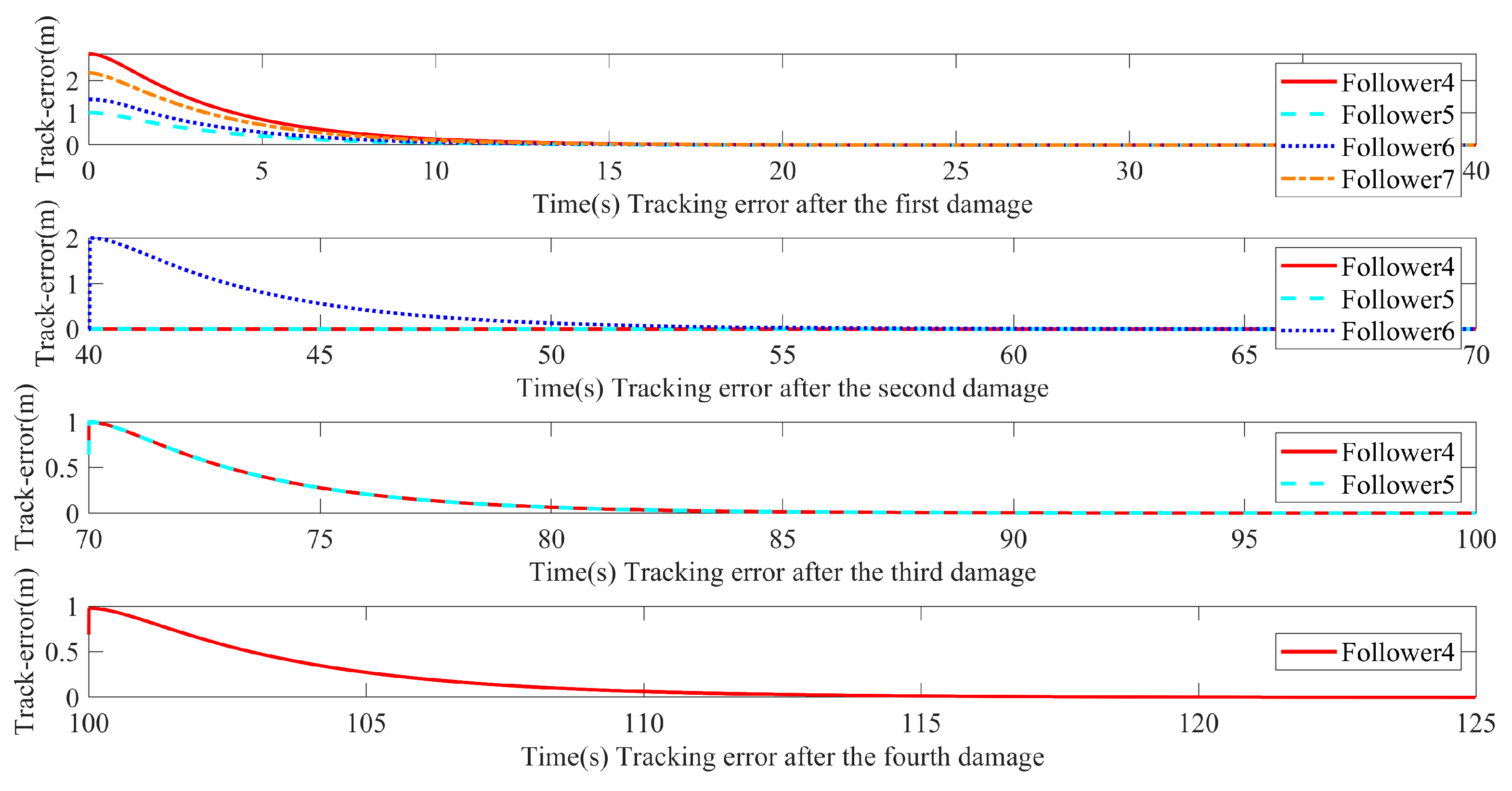
• A graphic library is innovatively established, and four possible multi-agent formation configurations are designed. After the failure of a single agent, topology images can be searched and dispatched in the graphic library according to the number of remaining agents, which can help the multi-agent system quickly establish a new configuration.
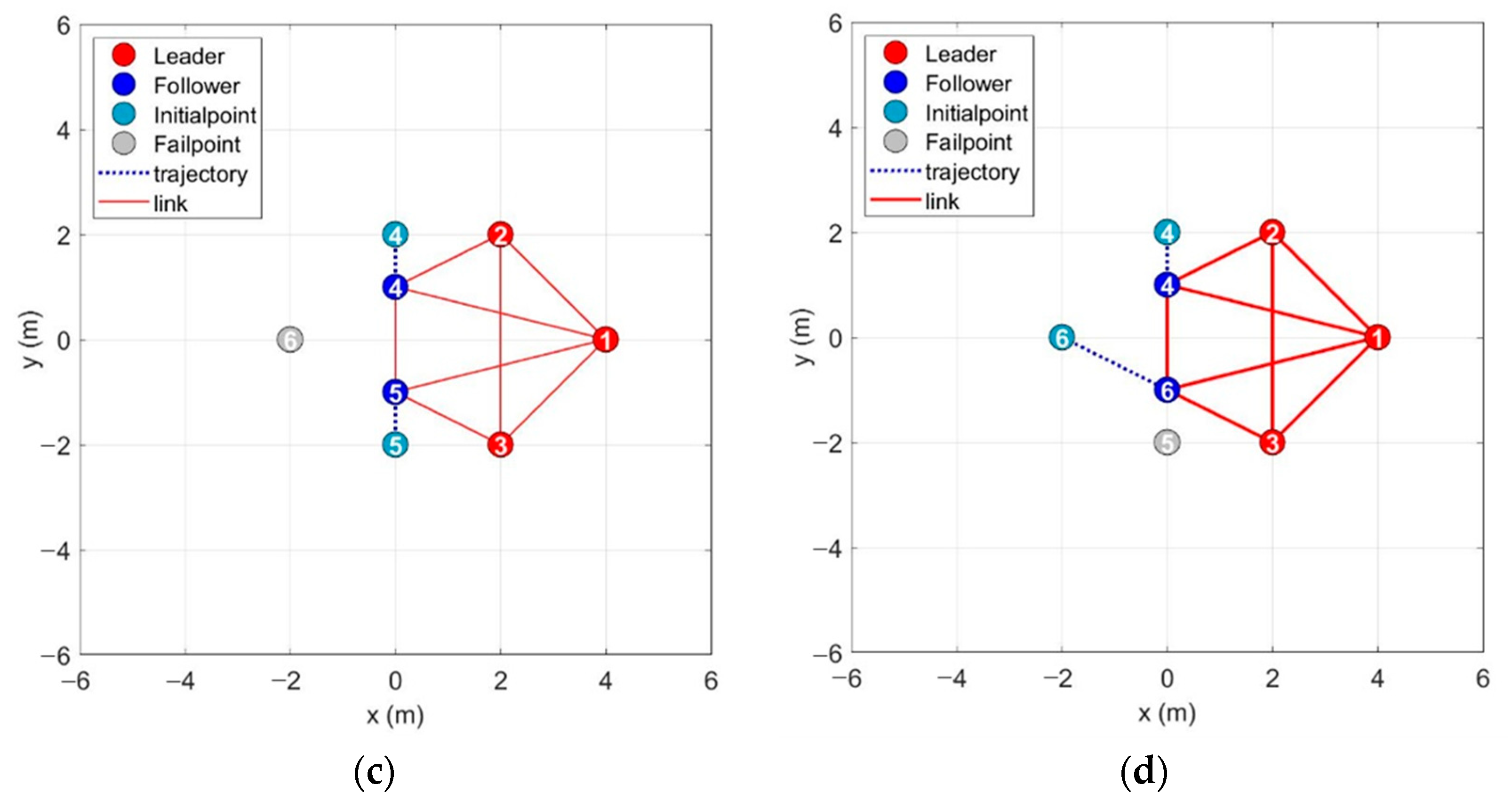
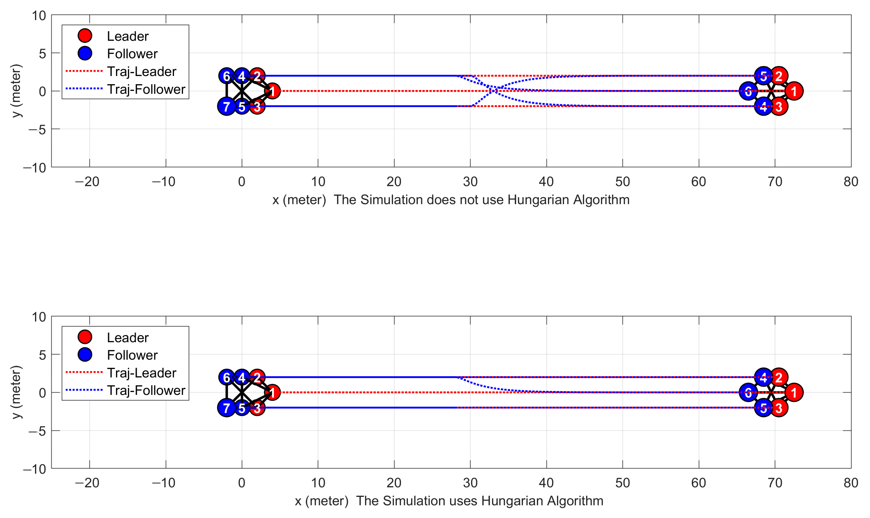
• The improved Hungarian algorithm is adopted to plan the target points so that each agent in the system can obtain specific target points in the formation using the ideal of ranking and a gradient weighting factor in the auction algorithm to further save time in formation reconfiguration.
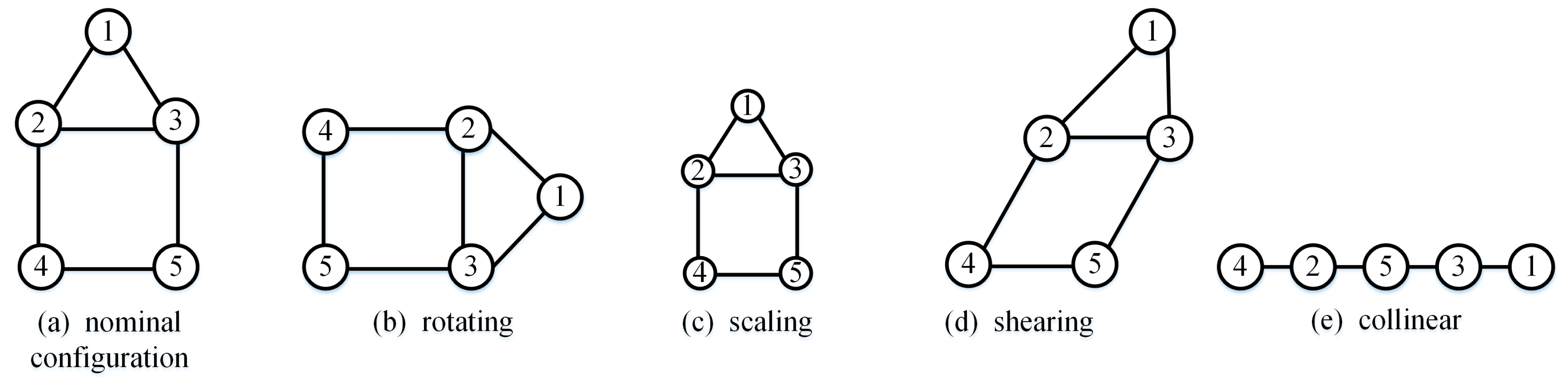
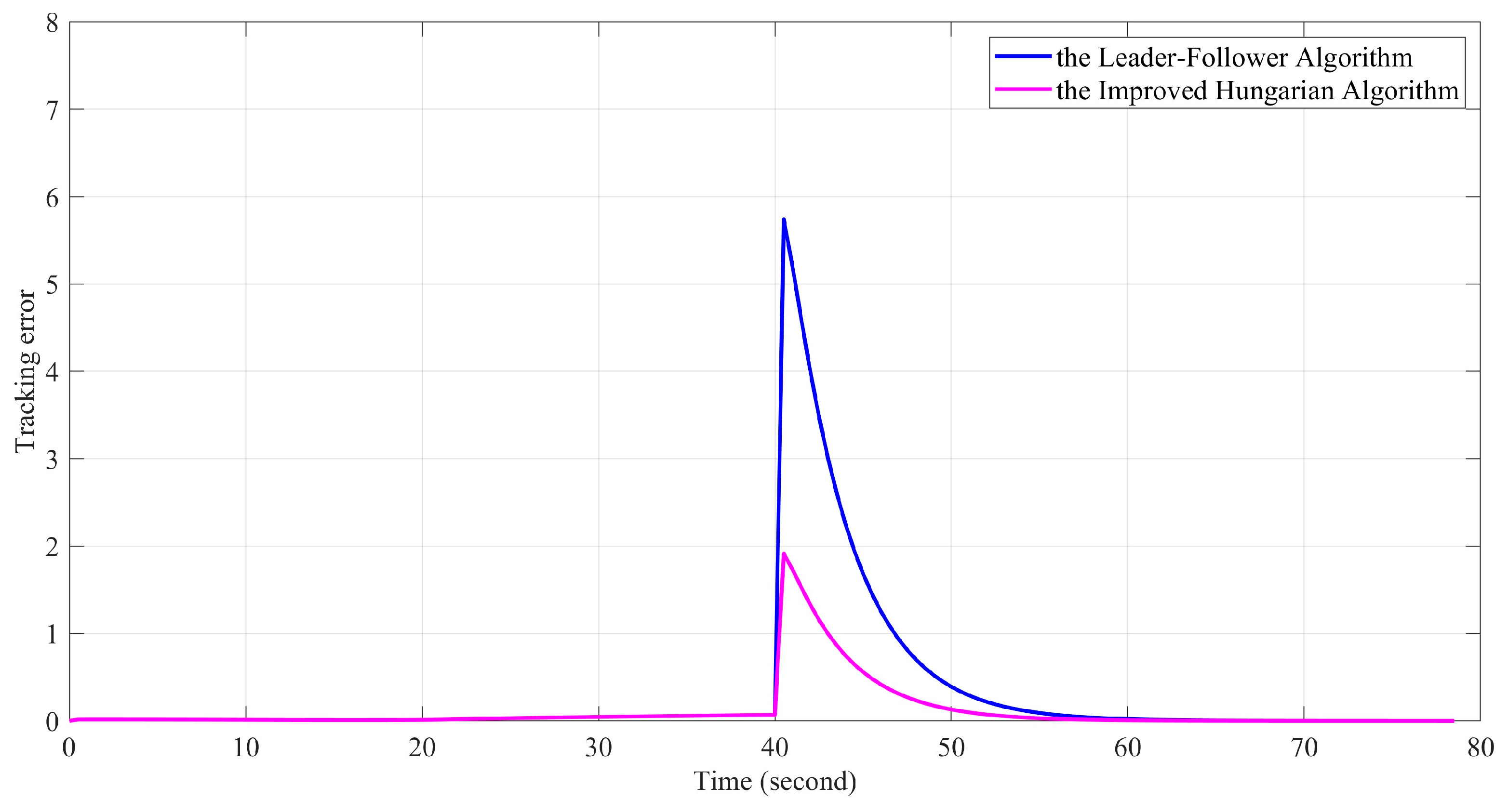
• In each topological cycle, a time-varying topological formation control law based on consistency theory is established. The control law can quickly reduce the tracking error to form a nominal configuration, and the stability of the formation reconfiguration system in a single time interval is proved by using the Lyapunov function.

The framework for the rest of this article is as follows. The second section first provides the concept of graph theory and the definition of time-varying target formations. The third section designs different numbers of time-varying formation topology configurations and builds corresponding graphics libraries. For multi-agent systems, the improved Hungarian algorithm is proposed to solve the problem of target position assignment after topology switching. The multi-agent formation reconstruction control strategy and stability analysis of the multi-agent systems are also provided. The fourth section obtains simulation images of multi-agent systems collaborative formation and reconstruction. The fifth section summarizes this article.

2. Theoretical Basis of Time-Varying Target Formation

This section introduces the concept of graph theory and the connotation of affine transformation and defines the nominal formation configuration, as well as our control target, which lays the foundation for the subsequent design of time-varying target configuration.

In the formation control of multi-agent, the agents cannot communicate with each other directly, and the communication between them needs to be established through the network topology. Graph theory is a very useful tool for studying cooperation systems. As a result, a formation is usually modeled by a graph, with vertices corresponding to agents and edges corresponding to the specified distance between the agents [16]. A directed simple graph has $n$ vertices and $m$ edges. $G=(\nu ,\epsilon )$$\nu =\{1,2,\dots ,n\},\epsilon \subseteq \nu \times \nu$ are denoted as the vertex set and the edge set of the graph $G$, respectively, where $\left|\epsilon \right|=m$. Consider the set of neighbors of vertex $i$, represented by $N_i=\{j\in v:(i,j)\in \epsilon \}$.

Thus, a formation is represented as $(G,p)$, and the graph $G$ with its vertex $i$ map to $p_i$. To simplify the collaborative interaction and improve the efficiency of information transmission, we adopt a leader-follower formation control strategy, and the desired formation maneuver is sent only to the leaders. It is assumed that the first $n_l$ agents in the formation are called leaders and other $n_f=n-n_l$ agents are called followers. In this article, $l$ and $f$ are the variables for leader and follower [17].

Affine transformation can be regarded as a kind of linear transformation [18]. Such transformations can be expressed in the form of translation, rotation, scaling, shearing, or their combination as shown in Figure 1. Numbers 1–3 in Figure 1 represent different agents. Moreover, affine transformation has a characteristic that collinear (coplanar) points or parallel lines remain collinear (coplanar) and parallel after an affine transformation. Thus, the affine span can be translated to a linear space, whose dimension is the dimension of the affine span. Assuming that the dimension of this affine span is $d$, then these points can affinely span in $R^d$. In addition, for affine span figures, the configuration will be changed when shearing or scaling in different directions.

Given a set of points ${\left\{p_i\right\}}_{i=1}^n$ in $R^d$, the affine span of these points (called $S$) can be expressed as

$$S=\{{\displaystyle \sum _{i=1}^n{a}_i{p}_i:a_i\in R },{\displaystyle \sum _{i=1}^n{a}_i=1}\}$$

(1)

Let the configuration matrix $P\in R^{n\times d}$ and an augmented matrix $\overline{P}\in R^{n\times (d+1)}$ be

$$P(p)=\left[\begin{array}{l}{p}_1^T\\ ⋮\\ p_n^T\end{array}\right],\overline{P}(p)=\left[\begin{array}{cc}{p}_1^T& 1\\ ⋮& ⋮\\ p_n^T& 1\end{array}\right]=\left[P(p),1_n\right]$$

(2)

where $1_n\triangleq {[1,\cdots ,1]}^T\in R^n$. By definition, if and only if the rows of $P(p)$ are linearly independent, ${\left\{p_i\right\}}_{i=1}^n$ are affinely independent. Because $P(p)$ has $d+1$ columns, there exist at most $d+1$ points that are affinely independent in $R^d$.

To achieve the formation control, a leader–follower multi-agent is needed to track time-varying goal configurations, as described below.

Definition 1 (Target formation).

The time-varying configuration of the target formation has the form of

$$p^{\ast }(t)=[I_n\otimes A(t)]r+1_n\otimes b(t)$$

(3)

where $r={[r_1^T,\cdots ,r_n^T]}^T={[r_l^T,r_f^T]}^T\in R^{dn}$ is a constant configuration, and $A(t)\in R^{d\times d}$, $b(t)\in R^d$ are continuous of $t$. The desired position of the agent $i\in v$  in the target formation is

$$p^{\ast }(t)=A(t)r+b(t)$$

(4)

In the above equation, $r$ is the typical geometric configuration that needs to be maintained during the formation process and $(G,r)$ is the nominal formation. In fact, the target configuration is an affine transformation of the nominal configuration that varies with time. There is a one-to-one correspondence between the positions of the different leaders and the affine transformations $(A,b)$. As a consequence, the affine transformation of the entire formation can be achieved by controlling the position of the leader. The objective of this paper is to control the multi-agent tracking the time-varying target formation and satisfy $p(t)\to p^{\ast }(t)$ during every split time.

In this article, there is no independent control law for leaders because we assume that leaders can be well controlled by humans or some intelligent program. It is known that the leader’s position corresponds to the expected value in the target configuration, that is $p_l(t)=p_l^{\ast }(t)$ for all $t$. Thus, our goal of control is to steer the followers to achieve $p_f(t)\to p_f^{\ast }(t)$ at different time intervals.

3. Design of Time-Varying Target Formation Control for Multi-Agent Systems Based on the Improved Hungarian Algorithm

3.1. Construction of Time-Varying Topology Formation Graphics Library

In the face of communication loss and other situations in complex environments, if the corresponding graphics are not generated in advance, it will take a lot of precious time to construct and reconstruct the formation, thus will miss the best opportunity. Therefore, if different numbers of target formations that may appear in advance are established, it will save time to call the graphics library when failure occurs at the first time, and a new reconstructed target topology can be efficiently and quickly established. In this section, we first introduce the concept of global rigidity and stress matrix based on graph theory to study the characteristics of formation configuration and describe these characteristics. The corresponding leaders for formation and reconstruction are selected, and the conditions required to construct a time-varying topological formation that meets the requirements are given.

Graph theory is a great mathematical tool for simplifying the characterization of multi-agent systems. Moreover, the rigidity [20] will reveal the uniqueness of the formation structure up to congruence. The generic configuration can be expressed by $q={[q_1^T,\cdots ,q_n^T]}^T\in R^{nd}$. A structure $(G,q)$ means a corresponding graph $G$ with its configuration $q$. A framework $(G,q)$ is rigid in $R^d$, if all the frameworks $(G,p)$ equivalent to $(G,q)$ and sufficiently close to $(G,q)$ are congruent to $(G,q)$ in $R^d$. If all the structures $(G,p)$ equivalent to $(G,q)$ are congruent to $(G,q)$, it is known as globally rigid in $R^d$. Moreover, if this congruent relationship holds in any higher-dimensional space $R^D\supset R^d$, it is universally rigid [21].

In addition, stress is also adopted to describe the robustness and stability of a framework. Essentially, stress means the direction of force with symbols and describes the force per unit length. $w$ represent the stress of $(G,q)$.

It is common to assign a scalar $w_{ij}=w_{ji}$ for each edge $(i,j)$ of a structure $(G,q)$. Next, $w\in R^m$ refers to the concatenated vector $w={(\cdots ,w_{ij},\cdots )}^T$.

Furthermore, if satisfies

$${\displaystyle \sum _{j\in N_i}{w}_{ij}(q_j-q_i)=0,\forall i\in \{1,\cdots ,n\}}$$

(5)

Then, it is defined that $w$ is equilibrium stress of $(G,q)$. Given $w$, there exists a stress matrix $\Omega \in R^{n\times n}$, for which ${\Omega }_{ij}=-w_{ij}$ for $i\ne j$ and ${\Omega }_{ii}={\displaystyle \sum _{i\ne j}{w}_{ij}}$ for $i=1,\cdots ,n$.

In the sequence, Lemmas 1–4 are given. These lemmas lead to conditions on the rank of the matrices that need to be satisfied for affine span as well as generic universal rigidity. In addition, the selection of the leader in the formation and the maximum upper bound on the number of edges are presented. These lemmas give constraints on the design of formation configurations and the establishment of graph libraries.

We will introduce Lemma 1 to define the rank condition for affine span.

Lemma 1 (Rank condition for affine span).

The set of points${\left\{p_i\right\}}_{i=1}^n$ affinely span$R^d$ if and only if $n\ge d+1$ and$rank(\overline{P}(p))=d+1$.

Lemma 2 [22] illustrates the definition of universal rigidity for a class of frameworks with generic configurations.

Lemma 2 (Generic universal rigidity).

Let $(G,q)$ be a generic framework on n vertices in  $R^d,d\le n-2$. Then $(G,q)$ is universally rigid if and only if there exists a positive semi-definite stress matrix $\Omega$ such that its rank is $n-d-1$.

Lemma 3 (Leader selection for affine localizability).

The nominal formation $(G,r)$ is affinely localizable if and only if  ${\left\{r_i\right\}}_{i\in v_l}$ affinely span $R^d$.

When there are exactly $d+1$ leaders, given any leader position $p_l$, there is always a solution $(A,b)$ to Equation (4). When there are more than $d+1$ leaders, the positions of leaders are interdependent. Otherwise, it is possible that there is no solution $(A,b)$ to Equation (4), because this equation is an overdetermined linear system. In this paper, we select three agents as leaders in formation and name them Leader 1, 2 and 3.

According to the formation dimension and the number of agents, Lemma 4 [23] gives the maximum number of edges of the time-varying formation topology. According to the calculation method, the upper bound of the number of lines between formations can be obtained.

Lemma 4 (The upper bound on the number of sides).

The number of members of the constructed tensegrity framework is bounded from above by

$$\left|\epsilon \right|\le (d+1)(n-\frac{d+2}{2}).$$

(6)

From the above Lemmas 1–4, we can obtain the conditions for the construction of time-varying topological formations.

Table 1. Graphics library formation information.

Formation Dimension	Number of Leaders	Total Number of Agents	Maximum Number of Sides	The Actual Number of Sides
2	3	7	15	12
2	3	6	12	11
2	3	5	9	8
2	3	4	6	6

. gives the formation information of the image and the above lemma is satisfied.

On this basis, we have designed the following formation configuration, as shown in Figure 2. Markers 1–7 in the figure correspond to agents with different numbers, and their locations represent the position of different agents in the formation. Due to Lemma 3, the choice of the leader is Agent 1–3.

We added the above formations to the graphics library so that the topological structure can be called immediately after random failure.

3.2. Improved Hungarian Algorithm Design

The problem of formation reconfiguration of multi-agent systems is considered when agents are randomly disabled in collaborative environments. If an agent randomly selects the target point, the path may be far away, and the overall energy consumption may be large. The Hungarian algorithm is often used in task allocation, so we use this algorithm to solve the problem of the allocation of target points after random failure. The algorithm usually traverses each target point to obtain the optimal allocation, which will take more time for urgent conditions. The auction algorithm combines the idea of auction algorithm ranking, and proposes a gradient weighting factor to improve the speed of target point allocation. Hence, this paper integrates the Hungarian algorithm with the auction algorithm and proposes an improved Hungarian algorithm. The expected target position can be quickly determined at the moment of failure, and the one-to-one correspondence between the agent and the target point in the expected formation can be ensured, which will help the system to increase the formation efficiency and improve the overall system reliability.

The agent matched one-to-one with the target location can be briefly described as follows: there are N agents performing tasks on N target points and a single agent is allowed to reach only one of the planar locations. Then the model of the formation target assignment problem for a multi-agent system based on matrix maps can be described as follows. The decision variables are defined by:

$$l(i,j)=\left\{\begin{array}{l}1 \mathit{i}\mathrm{th} \mathrm{agent} \mathrm{assigned} \mathrm{to} \mathrm{the} \mathit{j}\mathrm{th} \mathrm{point}\\ 0 \mathit{i}\mathrm{th} \mathrm{agent} \mathrm{doesn}’\mathrm{t} \mathrm{assigned} \mathrm{to} \mathrm{the} \mathit{j}\mathrm{th} \mathrm{point} \end{array}\right.$$

(7)

$$\mathrm{Constraint} \mathrm{condition}: \left\{\begin{array}{l}{\displaystyle \sum _{i=1}^n{l}_{ij}=1}, j=1,2,\dots ,n\\ {\displaystyle \sum _{j=1}^n{l}_{ij}=1}, \mathrm{i}=1,2,\dots ,n\\ x_{ij}=1 \mathrm{or} 0\end{array}\right.$$

(8)

$$\mathrm{Target} \mathrm{function}: z=\min {\displaystyle \sum _{i=1}^n{\displaystyle \sum _{j=1}^n{C}_{ij}{l}_{ij}}}$$

(9)

The number 1 means that the allocation is complete, and the number 0 means that it is not allocated. $C={(C_{ij})}_{n\times n}$ is the distance matrix. $C_{ij}$ is the distance value between the $j\text{-}\mathrm{th}$ target point and the $i\text{-}\mathrm{th}$ agent. $L={(l_{ij})}_{n\times n}$ is the solution matrix of the agent target assignment. When its value is 1, it means that the location assignment between the $i\text{-}\mathrm{th}$ agent and the $j\text{-}\mathrm{th}$ target point has been completed. When its value is 0, it means that the $j\text{-}\mathrm{th}$ target point has not been assigned to the $i\text{-}\mathrm{th}$ agent. Equation (9) is used to represent the minimum total distance from the agent formation to all target points, and the distribution matrix is calculated on this basis.

For the assignment problem model, the conditions for the solution of the improved Hungarian algorithm are: (1) The objective function is the smallest; (2) The number of agent and target points is the same; (3) The efficiency is non-negative. The goal of the Hungarian algorithm is to find N zero elements in different rows and columns in the transformed distance matrix to optimize the assignment problem.

The distance between each point and the target position is calculated.

$$C_{ij}=\sqrt{{(d_i^x-d_j^x)}^2+{(d_i^y-d_j^y)}^2}$$

(10)

Among them, $d_i^x$ represents the X-axis coordinate of the $i\text{-}\mathrm{th}$ agent and $d_j^y$ represents the y-axis coordinate of the $j\text{-}\mathrm{th}$ target points. After traversing the distance from all points to the target point, the distance matrix is obtained. Each element of the original distance matrix is normalized in the form of $a_{ij}=[\frac{c_{ij}-c_{\min }}{c_{\max }-c_{\min }}]$ to obtain its equivalent distance matrix $A$.

$c_{\min }=\min \{c_{ij},i=1,\cdot \cdot \cdot ,n,j=1,\cdot \cdot \cdot ,n\};$$c_{\max }=\max \{c_{ij},i=1,\cdot \cdot \cdot ,n,j=1,\cdot \cdot \cdot ,n\};$ At this point the maximum element $E$ of the equivalent matrix $A$. At this time, the $i\text{-}\mathrm{th}$ row/column elements are sorted incrementally to get $[b_1,\cdot \cdot \cdot b_n]$, The combined weighted sum of each step of the gradient is calculated as follows:

$$\begin{array}{l}{S}_i={\displaystyle \sum _{j=2}^n\frac{b_j-b_{j-1}}{E^{j-1}}}={\displaystyle \sum _{j=2}^n\frac{b_j}{E^{j-1}}}-{\displaystyle \sum _{j=2}^n\frac{b_{j-1}}{E^{j-1}}}\\ ={\displaystyle \sum _{j=1}^n\frac{b_j}{E^{j-1}}}-{\displaystyle \sum _{j=1}^n\frac{b_j}{E^j}}-\frac{b_1}{E^0}+\frac{b_n}{E^n}\\ ={\displaystyle \sum _{j=1}^n\frac{(E-1)\cdot b_j}{E^j}}+\frac{b_n}{E^n}\end{array}$$

(11)

The initial treatment of the distance matrix is determined using the auction algorithm, where the sorted minimum is 0, i.e., $b_1=0$.

Since this paper adopts the leader-follower formation control strategy, and the selection of the leader has been given in the previous section, it is assumed that only the followers are damaged during the maneuver.

The distance matrix $C_{ij}$ is taken as an example to illustrate the concrete implementation steps of the improved Hungarian algorithm in the case of failure:

• Before each calculation, use conditional statements to judge, and check the number of agents in the system, and feedback the number of agents in the system;
• Determine whether the agent is disabled in the current system; if failed, skip to step (3); if not, skip to step (6);
• According to the number of smart bodies, find and call the corresponding number of formation configurations in the graphics library; use the formations of the graphics library to generate new adjacency matrix and stress matrix, and renumber the smart bodies in order;
• Set the distance matrix of the agent. The improved Hungarian algorithm traverses the distance between the agent and each target point and calculates the cost matrix. Find the minimum value of each row/column of the distance matrix, and subtract the minimum value of all the elements in this row/column at the same time to get a new distance matrix. The matrix is constantly reduced by rows and columns until the 0 element appears in each row and column. We sort the elements of each row and column, and calculate the weighting factors of each order. Then we adjust the sorting results of the elements in each row and column, according to the sorting value assigned above. The non-zero minimum value is subtracted from the unassigned rows and the column element ordering result is adjusted. The same calculation needs to be done for unassigned columns. The algorithm counts the comprehensive gradient weighted sum of elements in each row and column.

$$\begin{array}{l}S{R}_i={\displaystyle \sum _{j=1}^n\frac{(E-1)R{b}_j}{E^j}}+\frac{R{b}_n}{E^n}\\ S{C}_i={\displaystyle \sum _{j=1}^n\frac{(E-1)C{b}_j}{E^j}}+\frac{C{b}_n}{E^n}\end{array}$$

(12)

5.

Among them, $(R{b}_1,\cdot \cdot \cdot ,R{b}_n),(C{b}_1,\cdot \cdot \cdot ,C{b}_n)$ are the incremental sorting results of the $i\text{-}\mathrm{th}$ row and $i\text{-}\mathrm{th}$ column elements respectively. For the unallocated row and column elements, the weighted sum of the comprehensive gradients is sorted from large to small, and the row or column with the largest comprehensive gradient is selected for trial allocation. To reduce the order of the distance matrix, the algorithm deletes the rows and columns allocated above. If the number of rows of the distance matrix is less than or equal to the number of columns, the weighted sum of the comprehensive gradients of the unallocated column elements is sorted from large to small, and the column with the largest comprehensive gradient is selected for trial allocation. By deleting the rows and columns of the above allocation, the order of distance matrix is reduced. Repeat the above process to determine whether the end condition is met and obtain the allocation result.

6.

According to the method of the minimum objective function, the target points to be reconstructed is reprogrammed, and the desired position to be achieved is assigned;

7.

Based on the above numbering method, use the leader-follower control law based on the consensus algorithm to control the system to achieve the formation and reconstruction of the overall goal.

The process of the trial allocation part is as follows:

Step 1.

Initialize the algorithm and related parameters;

Step 2.

The number of rows and columns in the distance matrix was compared. If the number of rows and columns are equal, go to the next step. If the number of rows is larger, go to step5, otherwise go to step7.

Step 3.

We sort the comprehensive weighted values of each row and column from large to small, so that the subscript of the row (column) with the largest comprehensive weighted value is;

Step 4.

If the row (column) with the smallest element in the row (column) k of the distance matrix is i_k, j_k respectively, then assign the row i_k to column j_k and go to step9.

Step 5.

Sorting the combined weighted values of the rows from the largest to the smallest, and let the subscript of the row with the largest combined weighted value be k;

Step 6.

If the smallest element in row k of the distance matrix is located is j_k, and assign row k to column j_k and go to step9.

Step 7.

Sorting the combined weighted values of the columns from the smallest to the largest, and let the subscript of the column with the largest combined weighted value be;

Step 8.

If the smallest element in the column k of the distance matrix is in the column i_k, then assign the row k to the column i_k and go to step9.

Step 9.

End the target trial assignment.

Figure 3 shows the process of time-varying target formation after using the improved Hungarian algorithm.

The following will give the allocation and planning of the improved Hungarian algorithm when failure occurs in the static formation. It is more intuitive to understand the path planning scheme of the improved Hungarian algorithm. Numbers 1–7 in the figure represent different agents and their locations. The red circle and the blue circle denote the leader and the follower, respectively. The gray circle represents the failed agent, the blue-green circle represents the initial position of the filled-in agent, and the dashed line shows its moving trajectory under static conditions. Figure 4a,b are the different situations in which agents are disabled from seven to six, respectively. If they are disconnected in sequence, the best allocation scheme obtained using the improved Hungarian algorithm, in this case, is the fourth and fifth agents remaining unchanged and the sixth agent moving down according to the reconstructed formation in the graphics library, filling the vacant position. If the fourth agent is randomly disabled, the optimal allocation of the target point after replanning is that the sixth agent fills the fourth position, and the seventh agent moves up to fill the sixth empty position and reconstitutes the formation of six.

Figure 4c,d show two cases of the accidental failure of six agents, respectively. Using the improved Hungarian algorithm to redistribute the target points at the first time can significantly save the overall path cost and quickly form a new reconfiguration pattern.

3.3. Multi-Agent System Control Law Design Based on Graph Theory and Consistency Algorithm

The corresponding control law for the second-order integrator model is designed to solve the multi-agent affine maneuver formation in this section.

As a consequence, consider a network composed of $N$ agents in $R^d$ space, given $d\ge 2$ and $N\ge d+2$ in this system. For the switching topology, in the time period of $t\to \infty$, there are countless time intervals $[t_m,t_{m+1}),m\in Z$,where $t_0=0$ represents time zero. Assume that each time interval satisfies $t_{m+1}-t_m\ge T$, where $T>0$. At every time interval, there are $k+1$ non-overlapping sub-intervals $[t_{m_s},t_{m_{s+1}}),s=0,1,\cdots ,k$. It can be assumed that within each sub-interval $[t_{m_s},t_{m_{s+1}})$,the network topology $G_s$ (switching topology) is fixed until the next time sub-interval is entered. The corresponding stress matrix can be expressed as ${\Omega }_s,s=0,1,\cdots ,k$ [24].

Assumption 1 (Affine span of nominal formation).

For the nominal formation $(G_s,r_s)$, assume that ${\left\{r_{si}\right\}}_{i=1}^n$ affinely span $R^d$.

Based on the switching topology networks, $p_{si}\in R^d,i=\{1,2,\cdots ,N\}$ represents the position of agent $i$ in the s-th switching topology, and the position of the entire formation are denoted as $p_s={[p_{s1}^T,p_{s2}^T,\cdots ,p_{sN}^T]}^T\in R^{dN}$. Information is transferred between agents by switching topologies $G_s$.

Assumption 2 (Stress matrix of nominal formation).

Assume that the nominal formation $(G_s,r_s)$ has a positive-semidefinite stress matrix ${\Omega }_s$ satisfying $rank({\Omega }_s)=n-d-1$.

If the set of all multi-agents is defined as ${\mu }_s$, ${\mu }_{sl}=[1,2,\cdots ,N_l]$ express the leaders set and the follower set is ${\mu }_{sf}={\mu }_s/{\mu }_{sl}$.The formation of leader is $p_{sl}={[p_{s1}^T,p_{s2}^T,\cdots ,p_{s{N}_l}^T]}^T$, and the formation of follower is $p_{sf}={[p_{s{N}_{l+1}}^T,p_{s{N}_{l+2}}^T,\cdots ,p_{sN}^T]}^T$. Hence, the formation of the whole formation can be rewritten as $p_s={[p_{sl}^T,p_{sf}^T]}^T$. In this network, assuming that there is no information transfer between leaders, and the leaders can’t obtain the information of followers. From the-above mentioned analysis, the stress matrix can be divided as

$${\Omega }_s=\left[\begin{array}{cc}{\Omega }_{s_{ll}}& {\Omega }_{s_{lf}}\\ {\Omega }_{s_{fl}}& {\Omega }_{s_{ff}}\end{array}\right]=\left[\begin{array}{cc}0& 0\\ {\Omega }_{s_{fl}}& {\Omega }_{s_{ff}}\end{array}\right]$$

(13)

Definition 2 (Affine localizability).

The nominal formation $(G_s,r_s)$ is affinely localizable by the leaders if for any $p_s={[p_{sl}^T,p_{sf}^T]}^T\in A(r)$, $p_{sf}$ can be uniquely determined by $p_{sl}$.

The Definition 2 can be interpreted as if the formation is in $A(r)$, then the position of followers can be uniquely determined by the leaders. As a result, this definition guarantees that the followers can track any desired configuration.

Assumption 3 (Affine localizability of nominal formation).

Assume that the nominal formation $(G_s,r_s)$ is affinely localizable by the leaders.

Before the control law is designed, Assumptions 1–3 need to be satisfied. To satisfy Assumption 1, the multi-agent system must be affinely span in $R^d$. To satisfy Assumption 2, the nominal configuration needs to be universally rigid. For the purpose of Assumption 3, there are at least $d+1$ agents selected as leaders that capable of affine span $R^d$ in the nominal formation.

For a group of multi-agents, each agent using the double integrator model can be expressed as follows

$$\left\{\begin{array}{l}{\dot{p}}_{si}=v_{si}\\ {\dot{v}}_{si}=u_{si}\end{array}\right.$$

(14)

$v_{si}$ can be expressed as the velocity of the agent and $u_{si}$ indicates the control input that needs to be designed.

For the purpose of driving all agents to reach the formation control, the following distributed control laws are proposed as follow:

$$\begin{array}{l}{\dot{p}}_{si}=v_{si}\\ {\dot{v}}_{si}=-\frac{1}{{\gamma }_{si}}{\displaystyle \sum _{j\in N_i}{w}_{s_{ij}}}[k_p(p_{si}-p_{sj})+k_v(v_{si}-v_{sj})-{\dot{v}}_{sj}]\end{array}$$

(15)

where the non-singularity of ${\gamma }_{si}$ is ${\gamma }_{si}={\displaystyle \sum _{j\in N_i}{w}_{s_{ij}}}$. The adjacency matrix element $w_{s_{ij}}$ is time-varying for different formation topologies.

The control law (15) is designed according to the consensus protocols for tracking time-varying references in [25].

Proposition 1 (Non-singularity of γ_si).

Under Assumptions 1–3, ${\gamma }_{si}>0$ for all $i\in {\nu }_{sf}$.

In this article, $\overline{\Omega }$ are used to represent $\Omega \otimes I_d$. Based on the partition of leaders and followers, the associated stress matrix ${\overline{\Omega }}_s$ can be denoted as

$${\overline{\Omega }}_s=\left[\begin{array}{cc}{\overline{\Omega }}_{s_{ll}}& {\overline{\Omega }}_{s_{lf}}\\ {\overline{\Omega }}_{s_{fl}}& {\overline{\Omega }}_{s_{ff}}\end{array}\right]$$

(16)

where ${\overline{\Omega }}_{{\mathrm{s}}_{\mathrm{f}\mathrm{f}}}\in {\mathrm{R}}^{(\mathrm{d}{\mathrm{n}}_{\mathrm{s}\mathrm{f}})\times (\mathrm{d}{\mathrm{n}}_{\mathrm{s}\mathrm{f}})}, {\overline{\Omega }}_{{\mathrm{s}}_{\mathrm{f}\mathrm{l}}}\in {\mathrm{R}}^{(\mathrm{d}{\mathrm{n}}_{\mathrm{s}\mathrm{f}})\times (\mathrm{d}{\mathrm{n}}_{\mathrm{s}\mathrm{l}})}$.

It is assumed that ${\overline{\Omega }}_{s_{ff}}$ is positive definite, thus we can obtain $p_{sf}^{\ast }(t)=-{\overline{\Omega }}_{s_{ff}}^{-1}{\overline{\Omega }}_{s_{fl}}{p}_{sl}^{\ast }(t)$ and $v_{sf}^{\ast }(t)={\overline{\Omega }}_{s_{ff}}^{-1}\overline{\Omega }{}_{s_{fl}}v{}_{sl}^{\ast }(t)$, respectively.

For $\underset{t\to \infty }{\lim }{v}_{s_l}(t)=v_{s_l}^{\ast }(t)$ and $\underset{t\to \infty }{\lim }{p}_{s_l}(t)=p_{s_l}^{\ast }(t)$, the position tracking error and the speed tracking error of the follower are expressed as

$$\begin{array}{l}{\delta }_{s_{pf}}(t)=p_{sf}(t)-p_{sf}^{\ast }(t)=p_{sf}(t)+{\overline{\Omega }}_{s_{ff}}^{-1}\overline{\Omega }{}_{s_{fl}}p{}_{sl}^{\ast }(t)\\ {\delta }_{s_{vf}}(t)=v_{sf}(t)-v_{sf}^{\ast }(t)=v_{sf}(t)+{\overline{\Omega }}_{s_{ff}}^{-1}\overline{\Omega }{}_{s_{fl}}v{}_{sl}^{\ast }(t)\end{array}$$

(17)

3.4. Stability Analysis of Time-Varying Topology Formation

In this section, based on the second-order integrator model, it is provided how the control law of the swarm reaches a steady state in segment interval, and finally realizes affine formation maneuver control. That is, the distributed control laws $u_{si}(t)$ for the follower makes the final realization of ${\delta }_{s_{pf}}(t)\to 0,{\delta }_{s_{vf}}(t)\to 0$. The following are the stability analysis of the control laws (15).

Multiplying ${\gamma }_{si}$ on both sides of (15) gives

$$\begin{array}{l}{\displaystyle \sum _{j\in N_i}{w}_{s_{ij}}({\dot{v}}_{si}-{\dot{v}}_{sj})}\\ ={\displaystyle \sum _{j\in N_i}{w}_{s_{ij}}[-k_p(p_{si}-p_{sj})}-k_v(v_{si}-v_{sj})]\end{array}$$

(18)

The matrix-vector forms are expressed as

$$\begin{array}{l}{\overline{\Omega }}_{s_{ff}}{\dot{v}}_{sf}+{\overline{\Omega }}_{s_{fl}}{\dot{v}}_{sl}^{\ast }\\ =-k_p({\overline{\Omega }}_{s_{ff}}{p}_{sf}+{\overline{\Omega }}_{s_{fl}}{p}_{sl}^{\ast })-k_v({\overline{\Omega }}_{s_{ff}}{v}_{sf}+{\overline{\Omega }}_{s_{fl}}{v}_{sl}^{\ast })\end{array}$$

(19)

Because of ${\delta }_{s_{pf}}(t)=p_{sf}(t)+{\overline{\Omega }}_{s_{ff}}^{-1}\overline{\Omega }{}_{s_{fl}}p{}_{sl}^{\ast }(t)$, ${\delta }_{s_{vf}}(t)=v_{sf}(t)+{\overline{\Omega }}_{s_{ff}}^{-1}\overline{\Omega }{}_{s_{fl}}v{}_{sl}^{\ast }(t)$, so

$${\overline{\Omega }}_{s_{ff}}{\dot{v}}_f+{\overline{\Omega }}_{s_{fl}}{\dot{v}}_{sl}^{\ast }=-k_p{\overline{\Omega }}_{s_{ff}}{\delta }_{s_{pf}}-k_v{\overline{\Omega }}_{s_{ff}}{\delta }_{s_{vf}}$$

(20)

Multiplying both sides by ${\overline{\Omega }}_{s_{ff}}^{-1}$, after shifting the term, we get ${\dot{v}}_{sf}=-k_p{\delta }_{s_{pf}}-k_v{\delta }_{s_{vf}}-{\overline{\Omega }}_{s_{ff}}^{-1}{\overline{\Omega }}_{s_{fl}}{\dot{v}}_{sl}^{\ast }$, and Formula (20) can be denoted as

$${\dot{\delta }}_{s_{vf}}={\dot{v}}_{sf}+{\overline{\Omega }}_{s_{ff}}^{-1}{\overline{\Omega }}_{s_{fl}}{\dot{v}}_{sl}^{\ast }=-k_p{\delta }_{s_{pf}}-k_v{\delta }_{s_{vf}}$$

(21)

As a result, the error dynamics can be written as

$$\left[\begin{array}{l}{\dot{\delta }}_{s_{pf}}\\ {\dot{\delta }}_{s_{vf}}\end{array}\right]=\left(\begin{array}{cc}0& I\\ -k_{p}I& -k_{v}I\end{array}\right)\left[\begin{array}{l}{\delta }_{s_{pf}}\\ {\delta }_{s_{vf}}\end{array}\right]$$

(22)

Define ${\phi }_s={\left[{\delta }_{s_{pf}}^T,{\delta }_{s_{vf}}^T\right]}^T$, and $W_s$ is the state matrix containing the control gain $k_p,k_v$.

The eigenvalue of the state matrix can be derived as ${\lambda }_s=(-k_v\pm \sqrt{k_v^2-4k_p})/2$, which always has the negative real part for any $k_v,k_p>0$. Thus $W_s$ is the Hurwitz matrix, and ${\phi }_s$ can converge to zero.

The global and exponential convergence follows. Through the above analysis, it can be concluded that the number of agents can achieve the expected configuration under the condition of switching topology.

4. Simulation Analysis of Switching Topology Formation

In this part, we validate the effectiveness of our proposed distributed control laws in the above sections. We carry out the simulation for the agents with the double integrator model (14) and the corresponding parameters are shown below.

Firstly, we consider the formation system with seven agents, where there exist four followers labeled 4, 5, 6, 7 and 3 leaders labeled 1, 2, 3. The initial positions of the seven agents are

$$q^{\ast }=\left[\begin{array}{ccccccc}4& 2& 2& 0& 0& -2& -2\\ 0& 2& -2& 2& -2& 2& -2\end{array}\right]$$

(23)

In addition, set the initial velocity of the multi-agent systems to 0. Let the control parameter be chosen as $k_p=0.5$ and $k_v=2$, respectively. The step size and the simulation time are constructed as 0.01 s and 80 s. It is very clear to see that the three leaders are not collinear in the formation, therefore they can affinely span in the plane.

For simulations in a 2D plane, the required configuration is given in the figure below. According to the theorems and arguments given above, we calculate the weights of the formation configuration of the six agents, as shown below. It can be proven to be universal rigidity.

$$\begin{array}{l}{k}_{11}=k_{66}=-0.4339,\\ k_{22}=k_{33}=k_{44}=k_{55}=-0.6508\\ k_{25}=k_{52}=k_{34}=k_{43}=0.4881\\ k_{12}=k_{21}=k_{13}=k_{31}=k_{46}=k_{64}=0.3254\\ k_{16}=k_{61}=-0.2169,k_{24}=k_{42}=-0.1627\end{array}$$

(24)

In practice, the prescribed formation shapes at different times are depicted in Figure 5. Different numbers in the figure represent different agents, with red and blue being the leader and follower respectively. It can be clearly found that after a single agent is disabled, the leader–follower algorithms [19] need three agents to form the given configuration in the graph library, and the paths appear to cross. After the Improved Hungarian algorithm is added in this paper, there are some trade-offs in the calculation time of the whole algorithm. However, in terms of effectiveness, the method adopted in this paper makes the formation move from multiple agents to only a single one. A comparison of the tracking errors of the two algorithms is shown in Figure 6. The algorithm used in this paper has a shorter convergence time and the peak error is reduced by 3.826.

Table 2. Data comparison of different strategies.

Different Strategies	Total Path Cost	Steady-State Time	Tracking Error Peak Comparison
Using the Leader-Follower algorithms	68.15	63 s	5.742
Using the Improved Hungarian Algorithm	60.09	55 s	1.916

shows that the total path consumption is reduced by 8.06 m, the time to reach the steady state is reduced by 8 s, and the peak tracking error is reduced by 66.6%, which greatly improves the efficiency of formation reconstruction. In a more complex environment, this algorithm can save more fuel and improve the efficiency of large-scale formation reconstruction.

In order to simulate the damage of agents, the number of agents is gradually reduced from seven to only four. From zero to forty seconds, there exists seven agents. The followers are disconnected at 40, 70, and 100 s respectively. Assuming that in the ideal state, the leader will not be failed, and the remaining agents continue to complete the task. The various nominal formations in Figure 2b are constructed according to the second part of the article. Furthermore, the given graphs are fixed during the piecewise maneuvering process. The corresponding stress matrixes can be calculated in advance by using the method in [21]. Moreover, the stress matrixes are all positive semidefinite and satisfy $rank({\Omega }_s)=n-d-1$.

The figure below shows the construction and path changes of the topology graph of multiple agents when there is random damage in the time-varying formation topology.

The arbitrarily initial positions of the seven agents can be obtained as $q(0)=q^{\ast }+rand(2,7)$, where the desired positions of these agents are $q^{\ast }=\left[\begin{array}{ccccccc}4& 2& 2& 0& 0& -2& -2\\ 0& 2& -2& 2& -2& 2& -2\end{array}\right]$.

With these control parameters, the trajectory snapshots of the multi-agent system at different times are plotted in Figure 7. From the results, the formation changed three times in total by disabling one follower at a time in the simulation. At the initial moment t = 0, the agents are in random loose positions. With the formation control, the designed formation configuration can be formed at t = 17 s. We note that the formation converges to the desired position from a random initial formation shape at the beginning using the given control law. At around the 40 s, the formation changes the scale and geometric pattern. As can be seen from the figure, the three leaders change from a triangle to a line formation at around 100 s. It can be observed that no matter how the formation changes, the parallel or collinearity lines are still preserved during the formation control. The pink line under the trajectory graph is the tracking error image, which can gradually converge to 0 with each change of formation.

It can be clearly seen in Figure 8 that for the followers, the time-varying target formation would produce the corresponding tracking errors at 3 different time points (40 s, 70 s, 100 s). After adding the improved Hungarian algorithm to the target point position distribution, the tracking error is kept within a small range, and can converge to 0 as soon as possible. Figure 8 shows that the affine formation tracking error of followers converges to zeros within 16 s, 54 s, 83 s, and 109 s.

5. Conclusions

Focusing on the problem of time-varying formation control, this paper introduces algebraic graph theory to abstract the connection topology between agents. Combining the concept of affine transformations with universal rigidity, the relation is unique regardless of how the topology graph is affine transformed in linear space. To achieve the minimum fuel consumption, the improved Hungarian algorithm is used to reallocate the target position after topology switching. Moreover, the corresponding model library has been built to rapidly establish new target formation configurations in a collaborative environment. Our method can save the whole system energy and improve the efficiency of multi-agent reconstruction after failure. A distributed control law based on consensus theory and leader-follower is designed for the linear model, and its global stability is proved using the Lyapunov function. In the end, the feasibility of the proposed approach was proved by the numerical simulations in the time-varying target configuration case.

Plenty of appealing directions for future research remain. The time-varying topological formation control considered in this paper is only for a single disabled agent. For a more complex and realistic collaborative environment, it is necessary to study the system with heterogeneous dynamics and when multiple agents are randomly disconnected. In the process of large-scale multi-agent reconstruction, how to avoid dynamic obstacles and how to face unknown external disturbances is another important research topic. In addition, the time-varying topology formation reconfiguration method in this paper can also be applied in three-dimensional or higher-dimensional spaces in the future.

References

1. Tian, L.; Zhao, Q.; Dong, X. Time-varying Output Group Formation Traking for Heterogeneous Multi-agent Systems. Acta Aeronaut. Astronaut. Sin. 2020, 41, 323727. [Google Scholar]
2. Chen, Q.; Wang, Y.; Jin, Y.; Wang, T.; Nie, X.; Yan, T. A Survey of An Intelligent Multi-Agent Formation Control. Appl. Sci. 2023, 13, 5934. [Google Scholar] [CrossRef]
3. Wang, W.; Zhang, W.; Hu, Z. PI Strategy Based Time-Varying Formation Control of Multiple Heterogeneous Agents. Electron. Optics Control 2021, 28, 11–15+30. [Google Scholar]
4. Zhen, Q.; Wan, L.; Li, Y. Time-varying Formation Control and Disturbance Rejection for UAV-UGV Heterogeneous Swarm System. Acta Aeronaut. Astronaut. Sin. 2020, 41, 723767. [Google Scholar]
5. Thuy, N.; Bui, D.; Phung, M. Deployment of UAVs for Optimal Multihop Ad-hoc Networks Using Particle Swarm Optimization and Behavior-based Control. In Proceedings of the International Conference on Control, Automation and Information Sciences (ICCAIS), Hanoi, Vietnam, 21–24 November 2022; IEEE: Piscataway, NJ, USA, 2022; pp. 304–309. [Google Scholar]
6. Zhen, Q.; Wan, L.; Li, Y. Formation Control of a Multi-AUVs System Based on Virtual Structure and Artificial Potential Field on SE(3). Ocean Eng. 2022, 253, 111148.1–111148.12. [Google Scholar] [CrossRef]
7. Wang, J.; Gu, W.; Dou, L. Leader-Follower Formation Control for Multiple UAVs with Trajectory Tracking Design. Acta Aeronaut. Astronaut. Sin. 2020, 41, 88–98. [Google Scholar]
8. Riahifard, A.; Rostami, S.M.H.; Wang, J.; Kim, H.-J. Adaptive Leader-Follower Formation Control of Under-Actuated Surface Vessels with Model Uncertainties and Input Constraints. Appl. Sci. 2019, 9, 3901. [Google Scholar] [CrossRef]
9. Pan, W.; Jiang, D.; Pang, Y.; Li, Y. A Multi-AUV Formation Algorithm Combining Artificial Potential Field and Virtual Structure. Acta Armamentarii 2017, 38, 326–334. [Google Scholar]
10. Lee, G.; Chwa, D. Decentralized Behavior-based Formation Control of Multiple Robots Considering Obstacle Avoidance. Intell. Serv. Robot. 2018, 11, 127–138. [Google Scholar] [CrossRef]
11. Shi, P.; Yu, J.; Liu, Y. Robust Time-varying Output Formation Tracking for Heterogeneous Multi-agent Systems with Adaptive Event-triggered Mechanism. J. Frankl. Inst. 2022, 359, 5842–5864. [Google Scholar] [CrossRef]
12. Qi, H.; Zhang, M.; Yao, H. Formation Maintenance and Reconfiguration Algorithm Design for Small UAVs. Ordnance Ind. Autom. 2021, 40, 32–35. [Google Scholar]
13. Guo, X. Consensus Analysis and Synthesis of Multi-Agent with Several Communication Topologies. Ph.D. Thesis, Beijing University of Technology, Beijing, China, 2017. [Google Scholar]
14. Tian, L.; Hua, Y.; Dong, X.; Lu, J. Distributed Time-Varying Group Formation Tracking for Multiagent Systems With Switching Interaction Topologies via Adaptive Control Protocols. IEEE Trans. Ind. Inf. 2022, 18, 8422–8433. [Google Scholar] [CrossRef]
15. Li, J.; Yu, J.; Hua, Y.; Dong, X.; Zhang, R. Resilient practical time-varying formation tracking for multiagent systems with a leader of unknown input. In Proceedings of the 2022 17th International Conference on Control, Automation, Robotics and Vision (ICARCV), Singapore, 11–13 December 2022; IEEE: Piscataway, NJ, USA, 2022; pp. 739–745. [Google Scholar]
16. Han, Z.; Wang, L.; Lin, Z.; Zheng, R. Formation Control with Size Scaling Via a Complex Laplacian-Based Approach. IEEE Trans. Cybern. 2016, 46, 2348–2359. [Google Scholar] [CrossRef] [PubMed]
17. Wu, G.; Hammers, J. Leader-Following Consensus of Nonlinear Discrete-Time Multi-Agent Systems with Limited Bandwidth and Switching Topologies. Am. J. Clin. Pathol. 2019, 152, S76. [Google Scholar] [CrossRef]
18. Xu, Y.; Luo, D.; You, Y.; Duan, H. Affine Transformation Based Formation Maneuvering for Discrete-Time Directed Networked Systems. Sci. China Technol. Sci. 2020, 63, 73–85. [Google Scholar] [CrossRef]
19. Zhao, S. Affine Formation Maneuver Control of Multiagent Systems. IEEE Trans. Automat. Contr. 2018, 63, 4140–4155. [Google Scholar] [CrossRef]
20. Tan, W.; Huang, N.; Huang, C.; Yu, C.; Zhong, C. Fixed-Time Rigidity-Based 3-D Formation Maneuvering Control with Distributed Finite-Time Velocity Estimators. In Proceedings of the 2019 Chinese Control Conference (CCC), Guangzhou, China, 27–30 July 2019; IEEE: Piscataway, NJ, USA, 2019; pp. 3237–3242. [Google Scholar]
21. Yang, Q.; Sun, Z.; Cao, M.; Fang, H.; Chen, J. Construction of Universally Rigid Tensegrity Frameworks and Their Applications in Formation Scaling Control. In Proceedings of the 2017 36th Chinese Control Conference (CCC), Dalian, China, 26–28 July 2017; IEEE: Piscataway, NJ, USA, 2017; pp. 8177–8182. [Google Scholar]
22. Gortler, S.J.; Thurston, D.P. Characterizing the Universal Rigidity of Generic Frameworks. Discrete Comput. Geom. 2014, 51, 1017–1036. [Google Scholar] [CrossRef]
23. Yang, Q.; Cao, M.; Fang, H.; Chen, J. Constructing Universally Rigid Tensegrity Frameworks with Application in Multiagent Formation Control. IEEE Trans. Automat. Contr. 2019, 64, 381–388. [Google Scholar] [CrossRef]
24. Lin, Z.; Wang, L.; Chen, Z.; Fu, M.; Han, Z. Necessary and Sufficient Graphical Conditions for Affine Formation Control. IEEE Trans. Automat. Contr. 2016, 61, 2877–2891. [Google Scholar] [CrossRef]
25. Coogan, S.; Arcak, M. Scaling the Size of a Formation Using Relative Position Feedback. Automatica 2012, 48, 2677–2685. [Google Scholar] [CrossRef]
Figure 1. Affine transformation types of a nominal configuration [19].
Applsci 13 11581 g001
Figure 2. Reconstructed formations in the graphics library.
Applsci 13 11581 g002
Figure 3. Flow chart of time-varying formation based on improved Hungarian algorithm.
Applsci 13 11581 g003
Figure 4. Target allocation in static case. (a) The seventh agent in the sequence fails, leaving six agents. (b) A random fourth agent fails, leaving six agents. (c) The sixth agent in the sequence fails, leaving five agents. (d) A random fifth agent fails, leaving five agents.
Applsci 13 11581 g004aApplsci 13 11581 g004b
Figure 5. Comparison of path curves of the two strategies.
Applsci 13 11581 g005
Figure 6. Comparison of tracking errors of two strategies.
Applsci 13 11581 g006
Figure 7. Time-varying formation topology path diagram.
Applsci 13 11581 g007
Figure 8. Comparison of time-varying topological formation tracking errors.
Applsci 13 11581 g008