A Machine Learning Model for the Prediction of Concrete Penetration by the Ogive Nose Rigid Projectile

Abstract

In recent years, research interest has been revolutionized to predict the rigid projectile penetration depth in concrete. The concrete penetration predictions persist, unsettled, due to the complexity of phenomena and the continuous development of revolutionized statistical techniques, such as machine learning, neural networks, and deep learning. This research aims to develop a new model to predict the penetration depth of the ogive nose rigid projectile into concrete blocks using machine learning. Genetic coding is used in Python programming to discover the underlying mathematical relationship from the experimental data in its non-dimensional form. A populace of erratic formulations signifies the rapport amid dependent parameters, such as the impact factor (I), the geometry function of the projectile (N), the empirical constant for concrete strength (S), the slenderness of the projectile (λ), and their independent objective variable, X/d, where X is the penetration depth of the projectile and d is the diameter of the projectile. Four genetic operations were used, including the crossover, sub-tree transfiguration, hoist transfiguration, and point transfiguration operations on supervised test datasets, which were divided into three categories, namely, narrow penetration (X/d < 0.5), intermediate penetration (0.5 ≤ X/d < 5.0), and deep penetration (X/d ≥ 5.0). The proposed model shows a significant relationship with all data in the category for medium penetration, where R² = 0.88, and R² = 0.96 for deep penetration. Furthermore, the proposed model predictions are also compared with the most commonly used NDRC and Li and Chen models. The outcome of this research shows that the proposed model predicts the penetration depth precisely, compared to the NDRC and Li and Chen models.

1. Introduction

1.1. Research Background

In the 20th century worldwide, various studies were conducted to produce innovative concrete variations [1]. However, since the 19th century, ordinary concrete is still the foremost distinctive practical material and is commonly used to build structures against accidentally-occurring impact loads [1]. These accidentally-occurring impact loads, such as vehicle crashes, plane crashes, tsunami, tornadoes, and flying objects are the main sources of penetration in concrete [2]. Figure 1 shows the illustration of penetration that occurs due to ogive nose rigid projectile impacts on concrete structures [2].

The historical penetration depth prediction model, that was developed based on experimental data, showed that the USA most frequently used the Petry model/the modified Petry model to predict penetration depth into a concrete block [1,3]. The Petry model was initially developed in 1910 and is considered the oldest available empirical model in literature [1,3]. Later, the Petry model was modified by Q.M. Li in the S.I unit [1,3]. In 1941, the Ballistic Research Laboratory (BRL) proposed the penetration prediction model [1,3]. Commencing in 1943, the Army Corp of Engineers also established the ACE model [1,3]. In 1946, the National Defense Research Committee (NDRC) proposed a model founded on the ACE model [1,3,4] The limitation of the NDRC hypothesis was that the NDRC model was used for rear penetration depths [1,3]. The NDRC also suggested a nose shape factor N* for projectiles, as mentioned in

Table A1. Previous studies equations for prediction of penetration depth with limitations.

References	Equation in S.I. Unit
Petry model [1,3,5]	$\frac{x}{d}=k\frac{M}{d^3}{\log }_{10}\left(1+\frac{V_o^2}{19,974}\right)$
Ballistic Research Laboratory (BRL) Model [1,3]	$\frac{x}{d}=\frac{1.33\times {10}^{-3}}{\sqrt{f_c}}\left(\frac{M}{d^3}\right)\hspace{0.17em}{d}^{0.2}{V}_o^{1.33}$
Army Corp of Engineers (ACE model) [1,3,23]	$\frac{x}{d}=\frac{3.5\times {10}^{-4}}{\sqrt{f_c}}\left(\frac{M}{d^3}\right)d^{0.2}{V}_o^{1.5}+0.5$
National Defense Research Committee (NDRC) Model [1,3,4,24]	$G=3.8\times {10}^{-5}\frac{N^{*}M}{d\sqrt{f_c}}{\left(\frac{V_o}{d}\right)}^{1.8}$	$G={\left(\frac{x}{2d}\right)}^2$	$\frac{x}{d}$ ≤ 2
		$G=\frac{x}{d}-1$	$\frac{x}{d}$ > 2
		$\frac{x}{d}=2G^{0.5}$	G ≥ 1
		$\frac{x}{d}=G+1$	G < 1
Ammann and Whitney model [1,3]	$\frac{x}{d}=\frac{6\times {10}^{-4}}{\sqrt{f_c}}{N}^{*}\left(\frac{M}{d^3}\right)d^{0.2}{V}_o{}^{1.8}$
Whiffen model [1,3,25]	$\frac{x}{d}=\left(\frac{2.61}{f_c^{0.5}}\right)\left(\frac{M}{d^3}\right){\left(\frac{d}{a}\right)}^{0.1}{\left(\frac{V_o}{533.4}\right)}^n$	$n=\frac{97.51}{f_c^{0.25}}$
Kar Model [1,3,26,27]	$G=3.8\times {10}^{-5}\frac{N^{*}M}{d\sqrt{f_c}}{\left(\frac{E}{E_s}\right)}^{1.25}{\left(\frac{V_o}{d}\right)}^{1.8}$	$\frac{x}{d}=2G^{0.5}$	G ≥ 1
		$\frac{x}{d}=G+1$	G < 1
UKAEA model [1,3,28]	$G=3.8\times {10}^{-5}\frac{N^{*}M}{d\sqrt{f_c}}{\left(\frac{V_o}{d}\right)}^{1.8}$	$\frac{x}{d}=0.275-{\left[0.0756-G\right]}^{0.5}$	G ≤ 0.0726
		$\frac{x}{d}={\left[4G-0.242\right]}^{0.5}$	0.0726 ≤ G ≤ 1.06
		$\frac{x}{d}=G+0.9395$	G ≥ 1.06
		$G=0.55\left(\frac{x}{d}\right)-{\left(\frac{x}{d}\right)}^2$	$\frac{x}{d}$ < 0.22
		$G={\left(\frac{x}{2d}\right)}^2+0.0605$	$0.22 \le \frac{x}{d}$ ≤ 2.0
		$G=\frac{x}{d}-0.9395$	$\frac{x}{d}$ ≥ 2.0
Haldar and Hamieh model [1,3,6]	$\frac{x}{d}=0.2251I_a+0.0308$	$I_a=\frac{M{N}^{*}{V}_o^2}{f_c{d}^3}$	0.3 ≤ Ia ≤ 4.0
	$\frac{x}{d}=0.0567I_a+0.6740$		4.0 ≤ Ia ≤ 21
	$\frac{x}{d}=0.0299I_a+1.1875$		21 ≤ Ia ≤ 455
Adeli and Amin Model [1,3]	$\frac{x}{d}=0.0416+0.1698I_a-0.0045I_a^2$	$I_a=\frac{M{N}^{*}{V}_o^2}{f_c{d}^3}$	for 0.3 ≤ Ia ≤ 4
	$\frac{x}{d}=0.0123+0.196I_a-0.008I_a^2+0.0001I_a^3$		4 ≤ Ia ≤ 21
Hughes Model [1,3,7]	$\frac{x}{d}=0.19\frac{N_h{I}_h}{S}$	$I_h=\frac{M{V}_o^2}{f_t{d}^3}$	Ih < 3500
		$S=1.0+12.3l_n\left(1.0+0.03I_h\right)$
Healy and Weissman Model [1,3]	$G=4.36\times {10}^{-5}\left(\frac{E}{E_s}\right)\frac{N^{*}M}{d\sqrt{f_c}}{\left(\frac{V_o}{d}\right)}^{1.8}$	$\frac{x}{d}=2G^{0.5}$	G ≥ 1
		$\frac{x}{d}=G+1$	G < 1
CREIPI Model [1,3,29]	$\frac{x}{d}=\frac{0.0265N^{*}M{d}^{0.2}{V}_o^2\left[114-6.83\times {10}^{-4}{f}_c^{\frac{2}{3}}\right]}{f_c^{\frac{2}{3}}}\left[\frac{\left(d+1.25H_r\right)H_r}{\left(d+1.25H_o\right)H_o}\right]$
UMIST model [1,3]	$\frac{x}{d}=\left(\frac{2}{\pi }\right)\frac{N^{*}}{0.72}\frac{M{V}_o^2}{{\sigma }_t{d}^3}$
	${\sigma }_t\left(Pa\right)=4.2f_c\left(Pa\right)+135\times {10}^6+\left[0.014f_c\left(Pa\right)+0.45\times {10}^6\right]\hspace{0.17em}{V}_o$
Li and Chen Model [1,3,8,10]	$\frac{x}{d}=\sqrt{\frac{\left(1+\left(\raisebox{1ex}{$k\pi $}\!\left/ \!\raisebox{-1ex}{$4N$}\right.\right)\right)}{1+\left(\raisebox{1ex}{$I$}\!\left/ \!\raisebox{-1ex}{$N$}\right.\right)}\frac{4kI}{\pi }}$	$I=\frac{I^{*}}{S}=\frac{1}{S}\left(\frac{M{V}_o^2}{f_c{d}^3}\right)$ $N=\frac{\lambda }{N^{*}}=\frac{1}{N^{*}}\left(\frac{M}{l_c{d}^3}\right)$ $S=72f_c^{-0.5}$ $k=\left(0.707+\frac{h}{d}\right)$	$\frac{x}{d}$ ≤ 5
	$\frac{x}{d}=\frac{2}{\pi }N\ln \left[\frac{1+\left(\raisebox{1ex}{$I$}\!\left/ \!\raisebox{-1ex}{$N$}\right.\right)}{1+\left(\raisebox{1ex}{$k\pi $}\!\left/ \!\raisebox{-1ex}{$4N$}\right.\right)}\right]+k$		$\frac{x}{d}$ > 5
	$\frac{x}{d}=1.628{\left(\frac{\left(1+\left(\raisebox{1ex}{$k\pi $}\!\left/ \!\raisebox{-1ex}{$4N$}\right.\right)\right)}{1+\left(\raisebox{1ex}{$I$}\!\left/ \!\raisebox{-1ex}{$N$}\right.\right)}\frac{4kI}{\pi }\right)}^{1.395}$		x/d < 0.5
	$\frac{x}{d}=\sqrt{\frac{\raisebox{1ex}{$4kI$}\!\left/ \!\raisebox{-1ex}{$\pi $}\right.}{1+\left(\raisebox{1ex}{$I$}\!\left/ \!\raisebox{-1ex}{$N$}\right.\right)}}$	If N » 1	$\mathrm{for} \frac{x}{d}$ ≤ k
	$\frac{x}{d}=\frac{2}{\pi }N\ln \left(1+\frac{I}{N}\right)+\frac{k}{2}$		$\mathrm{for}\frac{x}{d}$ > k
	$\frac{x}{d}=1.628{\left(\frac{\frac{4kI}{\pi }}{1+\left(\raisebox{1ex}{$I$}\!\left/ \!\raisebox{-1ex}{$N$}\right.\right)}\right)}^{1.395}$		x/d < 0.5
	$\frac{x}{d}=\sqrt{\frac{4kI}{\pi }}$	When I/N « 1	$\frac{x}{d}$ ≤ k
	$\frac{x}{d}=\frac{k}{2}+\frac{2I}{\pi }$		$\frac{x}{d}$ > k
	$\frac{x}{d}=1.628{\left(\frac{4k}{\pi }I\right)}^{1.395}$		x/d < 0.5

. Later, Ammann and Whitney’s model was anticipated to foretell the penetration of concrete traceable to the effect of strenuously precipitated particles at comparatively sophisticated velocities [1,3]. According to Kennedy [5], the Ammann and Whitney model can be used for velocities over 1000 ft/s [1,3]. Whiffen further continued research in the British Road Research Laboratory in the United Kingdom, using experimental data acquired from World War II, and developed a prediction model for penetration depth [1,3]. Kar altered the NDRC model, employing reversion regarding the modulus of elasticity (E), where E is the modulus of elasticity of the projectile, and Es is the modulus of elasticity of steel [1,3]. In the United Kingdom, Barr recommended a UKAEA model by reforming the NDRC model derived from wide-ranging research on nuclear power plant structures [1,3]. The Haldar–Hamieh model [1,3,6] of penetration depth relies on the dimensionless impact factor (Ia), where and N* is the nose shape factor [1,3,6]. Adeli and Amin improved the impact factor (Ia), familiarized by Halder and Hamieh, using regression on Sliter’s experimental data [1,3]. Hughes revised the NDRC hypothesis and suggested a model where I_h is a non-dimensional impact factor [1,3] and N_h is a nose shape factor [1,3]. Hughes proposed that the tensile and compressive strength of the concrete (ft/fc) ratio is constant [1,3,7]. Hughes also showed the importance of the strain rate and the dynamic increase factor (DIF), represented by ‘S’ [1,3,7]. Healy and Weissman introduced a model for penetration depth by revising the NDRC and Kar models [1,3]. The CRIEPI Model, mentioned below in Table A1, assumes the thickness of the concrete barrier Hr = 20 cm (0.2 m) [1,3]. In 1985, the United Kingdom Nuclear Electronics (UKNE) began intrinsic research on the behavior of concrete structures resisting hard projectile penetration by creating the R3 Concrete Impact Working Party [1,3]. The UMIST model for penetration depth (X) improved the form with the reflection of the nose shape [1,3]. Li and Chen [1,3,8] further advanced Forrestal et al.’s [1,3,9] model and proposed a semi-empirical or semi-analytical model for penetration depth (X). The model is in a non-dimensional homogenous form, and these models are valid for an extensive scope of penetration depth, where I is the impact function, and N is the geometry function. $S=72f_c^{-0.5}$ is an empirical function of fc (MPa). The Li and Chen model is applicable for X/d ≥ 5.0 [2,4]. Li and Chen [1,3,8,10] recommended X/d < 5.0 for small-to-medium penetration depths, where h is the length of the nose of the projectile. In the case of narrow penetrations when X/d < 0.5, the penetration depth is given by [1,3,8,10]. Chen and Li [1,3,8,10] recommended a simplified model of X/d = 0.5(I) to predict the penetration depth for deep penetration. The details of the discussed models are given in Appendix A Table A1.

Since 2005, researchers turned their attention to developing models in terms of the required critical impact energy [1,2]. Furthermore, research also turned to the advancement of concrete, creating high-performance concrete (HPC), ultra-high-performance concrete (UHPC), and high-performance fiber-reinforced concrete (HPFRC). However, until today, normal concrete and normal reinforced concrete are still the most commonly used materials for the construction of structures. The revised interest of researchers on concrete penetration depth emerged in 2015, when Husseini and Dalvand implemented an evolution of the statistical model developing technique, the neural network, to develop a model for the prediction of the rigid projectile penetration depth in concrete. Furthermore, in 2021, research was conducted using gradient tree boosting machine learning to predict RC panel failure modes under impact loading. These two kinds of research emerged with the need for the redevelopment of the model, using advanced machine learning tools to develop a prediction model based on an extensive collection of experimental data. Therefore, this research is focused on developing a model based on an extensive collection of 257 experimental test data, using machine learning symbolic regression. Furthermore, the proposed prediction model is validated with the prediction of the NDRC and Li and Chen models, because, in the literature, the most prominent model used to predict penetration depth is the Li and Chen dimensionless model [1].

1.2. Research Motivation

Based on the literature, there is a need to modernize the penetration depth prediction model in recent years. This is mainly due to the complexity of penetration phenomena, where there is a continuous evolution of techniques, such as neural networks and machine learning, especially since concrete is still commonly used in structures [11,12].

In 2015, Husseini and Dalvand used a neural network on 70 experimental datasets taken to estimate the penetration depth in concrete targets using an ogive nose rigid projectile [8,10,13,14,15,16]. The neural network models have a very low rate of error and high correlation coefficients compared to the regression-based models [17]. In 2021, Thai et al. used gradient tree boosting machine learning to predict RC panel failure modes under impact loading. The accuracy of the prediction result was not as high as expected, due to the lack of data and the unbalance experimental output features. However, this new approach was recommended for further investigation [18].

1.3. Research Objectives

The main objective of this research is to develop a modernized model for predicting penetration depth using machine learning symbolic regression genetic programming in Python. The model can predict the penetration depth with greater accuracy on a wide range of 257 tests, compared with the NDRC and Li and Chen models. The total of 257 test datasets from [2,8,10,13,14,15,16,19] is divided into three categories of narrow penetration depths, where X/d < 0.5; intermediate penetration depth, where 0.5 < X/d < 5.0; and deep penetration, where X/d > 5.0. X is the penetration depth and d is the diameter of the projectile. The significance of this research is that a reasonable number of 257 test datasets are trained and tested using machine learning symbolic regression with a genetic programming crossover, sub-tree transfiguration, hoist transfiguration, and point transfiguration to develop a model with better accuracy. The proposed model further compares with the NDRC and Li and Chen equations.

2. Machine Learning Symbolic Regression Genetic Programming Using Python

An interpretable supervised machine learning symbolic regression was used to discover the fundamental scientific equation to describe a Python correlation. Symbolic regression discovers mathematical equations using genetic programming [20]. A populace of erratic formulations is used to signify rapport amid dependent parameters, such as the impact factor (I), the geometry function of the projectile (N), the empirical constant for concrete strength (S), the slenderness of projectile (λ) and their independent objective variable, X/d, where X is the penetration depth of the projectile and d is the diameter of the projectile. In the iterative process, the consecutive propagation of a series of events is progressed from its predecessor’s generation by choosing the populace’s adequate entities to undertake genetic maneuvers. Genetic encoding yields a sequence of entirely unplanned programs (or models) and further predicts scientific equations to express the relationship between the reliant and sovereign parameters [21]. Four genetic operations used in genetic programming are the crossover, sub-tree transfiguration, hoist transfiguration, and point transfiguration operations, as shown in Figure 2. A sub-tree is randomly selected from the front-runner of an event in the crossover method and is replaced with a randomly selected sub-tree, since it is the front-runner of one more event (Figure 2a). A sub-tree is randomly chosen from the front-runner of an event in the sub-tree mutation method, and it is replaced with a sub-tree that is generated randomly (Figure 2b). The hoist mutation method selects a sub-tree of a randomly selected sub-tree from the winner of a tournament, which replaces the previously chosen sub-tree (Figure 2c). The point mutation method randomly selects some nodes from the tournament winner and replaces them with other building blocks (Figure 2d).

Symbolic regression generates a populace of unplanned scientific formulations with independent data factors as variants [22]. This scientific formulation genus transfigures and emerges as innovative models via genetic encoding [22]. The resulting formulations endeavor to predict trial data by appraising the specified metric (e.g., mean absolute error, root mean-squared error, or mean-squared error) between the predicted and actual values as shown in Figure 3.

3. Data Analysis

The penetration of the projectile can be divided into three categories, namely, deep penetration (X/d ≥ 5.0), intermediate penetration (0.5 ≤ X/d < 5.0), and narrow penetration (X/d < 0.5), where X is the penetration depth and d is the projectile’s diameter [10]. Experimental data in dimensionless form, shown in

Table 1. Dimensionless data with penetration depths for regression analysis.

λ	S	N	I	(X/d)test	λ	S	N	I	(X/d)test
15.2	21	143.4	14.45	9.83	5.31	11.81	5.31	0.66	0.86
15.2	21	143.4	36.55	24.15	5.31	11.04	5.31	0.78	0.91
15.2	21	143.4	47.28	27.79	5.31	12.41	5.31	1.33	1.22
15.2	21	143.4	54.73	32.04	5.31	12.07	5.31	1.25	1.29
15.2	21	143.4	93.77	49.54	5.31	11.81	5.31	1.36	1.31
15.2	21	143.4	133.13	65.79	5.31	11.04	5.31	1.16	1.29
15.2	21	200	12.5	8.59	10.75	12.41	10.75	1.47	1.51
15.2	21	200	35.94	24.15	10.75	12.07	10.75	1.43	1.73
15.2	21	200	54.73	33.98	10.75	11.81	10.75	1.45	1.58
15.2	21	200	85.07	51.32	10.75	11.04	10.75	1.37	1.58
15.2	21	200	118.67	66.56	10.75	12.41	10.75	2.77	2.36
19.64	12	125.9	8.45	6.43	10.75	12.07	10.75	2.71	2.89
19.73	12	126.5	17.33	11.52	10.75	11.81	10.75	2.42	2.27
19.66	12	126	18.93	15.28	10.75	11.04	10.75	2.29	2.36
19.77	12	126.7	29.02	17.84	6.12	10.81	6.12	2.41	1.45
19.73	12	126.5	32.62	19.52	6.12	11.39	6.12	1.65	1.47
19.62	12	125.8	36.55	27.1	6.12	11.86	6.12	0.71	1
19.53	12	125.2	33.6	19.07	6.12	10.8	6.12	1.7	1.5
19.57	12	125.5	43.48	22.57	3.14	11.39	3.14	0.35	0.65
19.62	12	125.8	46.02	23.05	3.14	11.17	3.14	0.44	0.77
19.53	12	125.2	64.02	32.19	3.14	11.17	3.14	1.39	1.1
19.6	12	125.6	76.45	35.61	5.85	10.77	5.85	1.91	1.25
19.91	7	127.6	23.15	13.12	6.34	10.77	6.34	1.16	1.2
19.72	7	126.4	24.7	14.28	6.34	11.19	6.34	2.54	1.65
19.93	7	127.8	25.85	16.25
19.87	7	127.4	25.34	15.69	14.45	15	144.51	1.66	3.15
19.91	7	127.6	39.83	23.42	14.4	15	144.03	2.29	4.07
19.76	7	126.7	38.35	22.49	12.98	11.26	121.91	3.77	3.94
					14.44	15	135.65	3.42	5.51
15.2	15.2	143.4	21.95	13.16	14.31	15	134.43	3.42	5.91
15.2	15.2	143.4	34.62	19.35	12.96	11.26	121.69	5.05	4.99
15.2	15.2	143.4	56.3	34.83	12.93	11.26	237.71	6.47	8.01
15.2	15.2	143.4	75.08	42.57	14.47	15	266.01	4.86	7.61
15.2	15.2	143.4	96	58.05	12.97	11.26	121.79	6.55	5.91
15.2	15.2	143.4	118.24	65.79	14.5	15	136.15	5.36	8.14
15.2	15.2	200	20.28	13.16	14.28	15	134.12	6.62	9.58
15.2	15.2	200	39.47	20.9	14.47	15	135.89	6.66	9.06
15.2	15.2	200	54.45	31.73	19.64	12	125.69	8.46	6.43
15.2	15.2	200	76.9	44.12	12.97	11.26	121.83	9.08	6.96
15.2	15.2	200	99.95	58.82	14.58	15	136.91	6.94	9.97
15.2	15.2	200	128.38	68.11	14.45	15	135.68	9.41	12.6
24.84	8.6	234.3	21.43	14.78	14.49	15	136.09	9.61	12.34
24.84	8.6	234.3	39.63	23.65	14.49	15	136.09	9.71	12.21
24.84	8.6	234.3	71.31	37.44	14.46	15	135.78	9.71	13.39
24.84	8.6	234.3	90.72	46.8	12.97	11.26	238.38	13.37	12.99
24.84	8.6	234.3	103.09	45.32	13.02	11.26	122.23	13.89	12.34
24.84	8.6	234.3	110.97	46.31	19.91	7	127.44	23.15	13.12
24.52	10.5	231.3	17.28	12.13	19.72	7	126.18	24.7	14.28
24.52	10.5	231.3	20.95	13.77	19.87	7	127.16	25.34	16.25
24.52	10.5	231.3	31.29	18.36	19.94	7	127.58	25.93	15.69
24.52	10.5	231.3	44.64	25.57	24.64	10.5	231.41	17.36	12.13
24.52	10.5	231.3	68.09	34.43	14.47	15	266.07	12.26	16.4
24.52	10.5	231.3	70.99	40.33	24.84	8.6	233.31	21.42	14.78
24.52	10.5	231.3	85.31	46.23	14.54	15	136.5	12.32	15.49
24.52	10.5	231.3	107.23	57.38	24.63	8.7	231.3	21.97	14.14
24.52	10.5	231.3	120.29	64.26	24.61	7.9	231.13	24.51	15.08
24.52	10.5	231.3	151.92	66.56	19.73	12	126.25	17.33	11.52
					24.52	10.5	230.26	20.95	13.77
24.63	8.7	232.4	21.97	14.14	19.66	12	125.83	18.93	15.28
24.63	8.7	232.4	41.92	24.19	14.84	20.2	194.91	12.95	8.51
24.63	8.7	232.4	74.7	41.38	15.19	21	199.51	12.5	8.59
24.63	8.7	232.4	114.5	64.04	19.76	7	126.46	38.35	22.49
24.63	8.7	232.4	151.85	78.33	19.91	7	127.44	39.83	23.42
24.63	8.7	232.4	70.37	35.96	14.84	20.2	139.34	14.98	10.06
24.63	8.7	232.4	111.12	57.14	15.19	21	142.63	14.45	9.83
24.63	8.7	232.4	152.64	71.92	14.84	15.2	194.91	20.22	13.16
24.61	7.9	232.2	24.5	15.08	24.52	10.5	230.26	31.28	18.36
24.61	7.9	232.2	42.21	25.9	14.84	15.2	139.34	21.88	13.16
24.61	7.9	232.2	77.91	40.33	24.61	7.9	231.13	42.21	25.9
24.61	7.9	232.2	118.85	63.93	24.84	8.6	233.31	39.63	23.65
24.61	7.9	232.2	121.78	64.26	19.77	12	126.52	29.02	17.84
24.61	7.9	232.2	171.15	87.54	24.63	8.7	231.3	41.85	24.19
					19.73	12	126.25	32.62	19.52
39.69	11.02	39.69	0.18	0.71	19.53	12	125	33.6	19.07
3.48	11.1	3.48	0.15	0.56	19.62	12	125.55	36.55	27.1
3.48	11.1	3.48	0.15	0.66	24.56	10.5	230.69	44.71	25.57
2.45	11.1	2.45	0.15	0.41	19.57	12	125.27	43.48	22.57
3.48	11.1	3.48	0.17	0.61	14.84	15.2	139.34	34.52	19.35
2.45	11.1	2.45	0.15	0.34	19.62	12	125.55	46.02	23.05
2.45	12.22	2.45	0.24	1.31	14.84	15.2	194.91	39.37	20.9
2.93	12.22	2.93	0.15	0.32	24.63	8.7	231.3	70.37	35.96
2.45	12.22	2.45	0.17	0.41	24.84	8.6	233.31	71.31	37.44
2.94	12.22	2.94	0.2	0.78	24.61	7.9	231.13	78.42	40.33
3.48	12.22	3.48	0.27	0.73	24.63	9.04	231.3	68.77	49.75
3.48	12.22	3.48	0.22	0.49	24.63	9.04	231.3	69.81	60.39
2.45	12.22	2.45	0.3	0.57	24.63	8.7	231.3	74.7	41.38
2.45	12.22	2.45	0.08	0.07	24.58	10.5	230.84	68.24	34.43
2.94	12.22	2.94	0.3	0.54	24.52	10.5	230.26	70.98	40.33
3.48	11.34	3.48	0.3	1.47	14.84	20.2	194.91	37.24	23.99
2.45	11.34	2.45	0.33	0.95	15.19	21	199.51	35.93	24.15
2.94	11.34	2.94	0.1	0.1	14.84	20.2	139.34	37.88	23.99
2.94	11.34	2.94	0.22	0.44	15.19	21	142.63	36.55	24.15
2.45	11.76	2.45	0.4	0.75	19.53	12	125	64.02	32.19
13.04	11.76	13.04	0.38	0.5	24.84	8.6	233.31	90.72	46.8
4.6	11.76	4.6	0.25	0.66	14.84	15.2	194.91	54.29	31.73
2.45	11.76	2.45	0.27	0.26	14.84	15.2	139.34	56.12	34.83
13.04	11.76	13.04	0.37	2.15	24.84	8.6	233.31	103.07	45.32
2.45	11.76	2.45	0.1	0.21	24.56	10.5	230.69	85.46	46.23
4.6	11.76	4.6	0.11	0.36	19.6	12	125.41	76.45	35.61
0.83	10.6	0.83	0.09	0.32	24.61	7.9	231.13	116.93	64.26
1.63	11.67	1.63	0.2	0.95	24.61	7.9	231.13	118.86	63.93
0.83	12.13	0.83	0.16	1.04	24.84	8.6	233.31	110.94	46.31
0.69	11.25	0.69	0.08	0.54	24.61	7.9	231.13	121.79	64.26
0.69	11.41	0.69	0.04	0.13	24.63	8.7	231.3	111.12	57.14
1.05	11.1	1.05	0.05	0.34	14.84	20.2	139.34	48.85	27.86
0.53	10.6	0.53	0.06	0.23	15.19	21	142.63	47.14	27.79
0.95	11.41	0.95	0.28	0.34	24.63	8.7	231.3	114.5	64.04
0.95	10.74	0.95	0.35	0.55	24.5	10.5	230.12	107.15	57.38
0.7	11.67	0.7	0.24	0.5	14.84	15.2	139.34	74.85	42.57
0.7	11.25	0.7	0.35	1	14.84	20.2	139.34	56.73	31.73
0.56	11.03	0.56	0.14	0.5	14.84	20.2	194.91	56.73	34.06
96.15	14.28	96.15	5.25	3.6	15.19	21	142.63	54.74	32.04
96.15	14.51	96.15	10.97	5.8	15.19	21	199.51	54.74	33.98
96.63	12.29	96.63	1.14	1.2	14.84	15.2	194.91	76.67	44.12
96.63	10.99	96.63	2.09	1.6	24.66	10.5	231.56	121.02	64.26
96.63	10.96	96.63	2.23	2	24.63	8.7	231.3	151.85	78.33
96.63	11.14	96.63	1.92	1.7	24.63	8.7	231.3	152.64	71.92
5.02	11.13	5.02	0.04	0.09	24.61	7.9	231.13	171.16	87.54
5	12.67	5	0.07	0.25	14.84	15.2	139.34	95.7	58.05
5	12.17	5	0.3	1.13	24.61	7.9	231.13	185.72	92.79
5	12.34	5	0.23	0.38	14.84	15.2	194.91	99.65	58.82
5.05	12.74	5.05	0.39	0.56	24.56	10.5	230.69	152.18	66.56
5.56	15.31	5.56	0.03	0.06	14.84	20.2	194.91	88.14	51.08
5.65	13.93	5.65	0.03	0.05	15.19	21	199.51	85.05	51.32
5.65	13.93	5.65	0.06	0.04	14.84	15.2	139.34	117.88	65.79
5.61	12.9	5.61	0.1	0.12	14.84	15.2	194.91	127.99	68.11
5.65	13.93	5.65	0.14	0.14	14.84	20.2	139.34	97.18	49.54
10.46	13.93	10.46	0.06	0.06	15.19	21	142.63	93.77	49.54
10.46	13.93	10.46	0.1	0.06	14.84	20.2	194.91	122.96	66.56
5.31	12.41	5.31	0.83	0.95	14.84	20.2	139.34	137.97	65.79
5.31	12.07	5.31	0.79	1.02

, is used for the symbolic regression analysis to obtain a mathematical model [2,8,10,13,14,15,16,19]. The data’s dimensionless parameters include the impact factor $I=\left(\frac{M{V}_o^2}{f_c{d}^{3}S}\right)$, where M is mass of the rigid projectile, V_o is impacting projectile velocity, fc is the compressive strength of the concrete, d is the diameter of the rigid projectile, and $S=72f_c^{-0.5}$ is the empirical constant for concrete strength. The geometry function of the projectile is $N=\left(\frac{M}{l_c{d}^3{N}^{*}}\right)$, where M is the mass of the rigid projectile, N* is nose shape factor projectile, $l_c$ is the density of concrete, and d is the diameter of the rigid projectile. The slenderness of the projectile is $\lambda =\left(\frac{M}{l_c{d}^3}\right)$, where M is the mass of the rigid projectile, $l_c$ is the density of concrete, and d is the diameter of the rigid projectile. The empirical constant for concrete strength is $S=72f_c^{-0.5}$, and X/d refers to the dimensionless penetration depth ratio-to-projectile diameter. The dimensionless penetration X/d is taken as a dependent target variable, whereas I, N, λ, and S are independent variables or predictors.

The correlation among predictors is shown in Figure 4 as a correlation matrix. The correlations are calculated separately for narrow, medium, and deep penetration. N and λ values are identical in the narrow penetration data. Hence, the data have a perfect correlation of 1.0. S and N are also highly correlated. In the medium penetration data, N is highly correlated with I and λ. In the deep penetration data, the correlation among predictors is weak. A summary of the statistics of predictors for different penetration types is shown in

Table 2. Descriptive statistics of N, I, S, and λ in narrow, intermediate, and deep penetrations.

Statistics	Independent Variables
	I			N			λ			S
	Narrow	Intermediate	Deep	Narrow	Intermediate	Deep	Narrow	Intermediate	Deep	Narrow	Intermediate	Deep
Count	26	59	174	26	59	174	26	59	174	26	59	174
Mean	0.12	1.19	60.05	3.83	22.29	182.81	3.83	14.20	19.96	12.24	11.74	12.75
Std	0.074	1.15	44.29	2.60	39.85	47.24	2.60	25.93	7.30	1.24	0.89	4.55
Cov	0.62	0.97	0.74	0.68	1.79	0.26	0.68	1.83	0.37	0.10	0.08	0.36
Min	0.03	0.08	3.42	0.53	0.56	96.15	0.53	0.56	12.93	10.60	10.74	7.00
25%	0.06	0.30	23.15	2.45	3.14	135.94	2.45	3.14	15.19	11.34	11.10	8.70
50%	0.10	0.79	45.37	2.94	5.31	194.91	2.94	5.31	19.65	11.99	11.67	12.00
75%	0.15	1.68	90.72	5.43	10.75	231.30	5.43	10.75	24.61	12.84	12.15	15.20
Max	0.28	5.25	185.72	10.46	144.51	266.07	10.46	96.63	96.15	15.31	15.00	21.00

Std: standard deviation; Cov: coefficient of variation; 25%: 25th percentile (i.e., 25 percent of data is below this value); 50%: 50th percentile; 75%: 75th percentile.

.

In order to explore the distribution of predictors, a boxplot (or a box-and-whisker plot) of each predictor for the different penetration ranges is shown in Figure 5. The median is shown by the vertical line inside the box, whereas the left and right sides of the box are the first and third quartiles, respectively. Most of the data lie in the first and third quartiles, and the lines that are referred to as whiskers extend on the right and left sides of the box to indicate the range. There is a clear separation of I, N, and λ in the different penetration ranges. The median of S is the same for different penetration ranges, while there is more deep penetration data. More outliers in all predictors in the medium penetration are observed, as seen by the points plotted beyond the whiskers.

Figure 6, Figure 7 and Figure 8 show pair plots of the predictors for narrow, medium, and dense penetration ranges, respectively. The diagonals are density plots calculated from the data through a kernel density estimate (KDE) [20,21]. The KDE plots can be considered as smoothed histograms. The plots above the diagonal are scattered plots with bivariate KDE contours overlapping the scatter points. The bivariate KDE plot estimates the probability density of two variables. The shaded contours represent different density levels. The plots below the diagonal are scattered plots with linear regressions among predictors. In the narrow penetration range, the distribution of I, N, and S is skewed, with a high correlation between N and S. In the medium penetration range, the distribution of all predictors is skewed with a high correlation of N with I and λ, respectively. The I and S distributions are skewed in the deep penetration range, whereas N and λ have two modes. Furthermore, all predictors are weakly correlated in the deep penetration range.

4. Proposed Model Using Symbolic Regression in Python

Symbolic regression is performed using gplearn [22], which executes genetic encoding in Python through a scikit-learn stimulated and reconcilable application programming interface (API). The hyperparameters used for symbolic regression in gplearn are listed in

Table 3. The hyperparameters for symbolic regression in gplearn.

Parameter	Value
	EQ 1	EQ 2	EQ 3
population size	5000	5000	5000
generations	60	60	60
stopping_criteria	0.01	0.01	0.01
p_crossover	0.9	0.7	0.7
p_subtree_mutation	0.01	0.01	0.1
p_hoist_mutation	0.01	0.05	0.05
p_point_mutation	0.01	0.1	0.1
function_set	+, −, ×, ÷	+, −, ×, ÷, √	+, −, ×, ÷
tournament size	25	25	25
parsimony_coefficient	0.0003	0.002	0.003
metric	MAE	MAE	MAE
const_range	(−5, 5)	(−5, 5)	(−5, 5)

The following is an explanation of the hyperparameters: population size: number of mathematical formulas in each generation; generations: maximum number of generations; stopping_criteria: MAE value that program stops; p_crossover: crossover probability; p_subtree_mutation: subtree mutation probability; p_hoist_mutation: hoist mutation probability; p_point_mutation: point mutation probability; function_set: building blocks containing mathematical operators; parsimony_coefficient: a constant that penalizes large individuals by adjusting their MAE to make them less favorable for selection; metric: measures how well an individual fits; const_range: the range of constants included in the model.

. The experimental dataset of 257 observations [2,8,10,13,14,15,16,19] as shown in Table 1, is further separated according to the penetration type. Datasets belonging to narrow, intermediate, and deep penetrations consist of 26, 59, and 174 data observations, respectively. Symbolic regression is performed separately for each dataset to obtain the underlying mathematical expressions to describe the best relationship. For intermediate and deep penetration datasets, 70% of data is used to construct the mathematical model (i.e., train the model), and 30% of data is used to test the mathematical model’s performance (i.e., test the model). Since data observations in the narrow penetration are small and consist of 26 data observations only, all data is used to construct the mathematical model. The hyperparameters used for symbolic regression in gplearn are shown in Table 3.

The mathematical model obtained for narrow, medium, and deep penetration datasets from symbolic regression is shown in the Figure 9, Figure 10 and Figure 11 as expression tress (ETs).

The proposed equations, obtained from symbolic regression, can be re-written in mathematical form, as follows.

$$\frac{x}{d}=\left(I-\frac{3I}{N}\right)\left(1.179-\frac{3I}{N}\right) \mathrm{for} \frac{x}{d}<0.5$$

(1)

$$\frac{x}{d}=I^3+\left(I-1.0\right)\left(N-\lambda \right)+0.202 \mathrm{for} 0.5<\frac{x}{d}<5.0$$

(2)

$$\frac{x}{d}=0.5I+3.324 \mathrm{for} \frac{x}{d}>0.5$$

(3)

5. Results and Discussion

The mathematical model performances are shown in Figure 12, Figure 13 and Figure 14 and

Table 4. Statistics of previous studies compared to the proposed study.

Metric	Comparison of Performance between Different Equations
	NDRC	Barr	Li and Chen	Sym. Reg.a (Present Study)
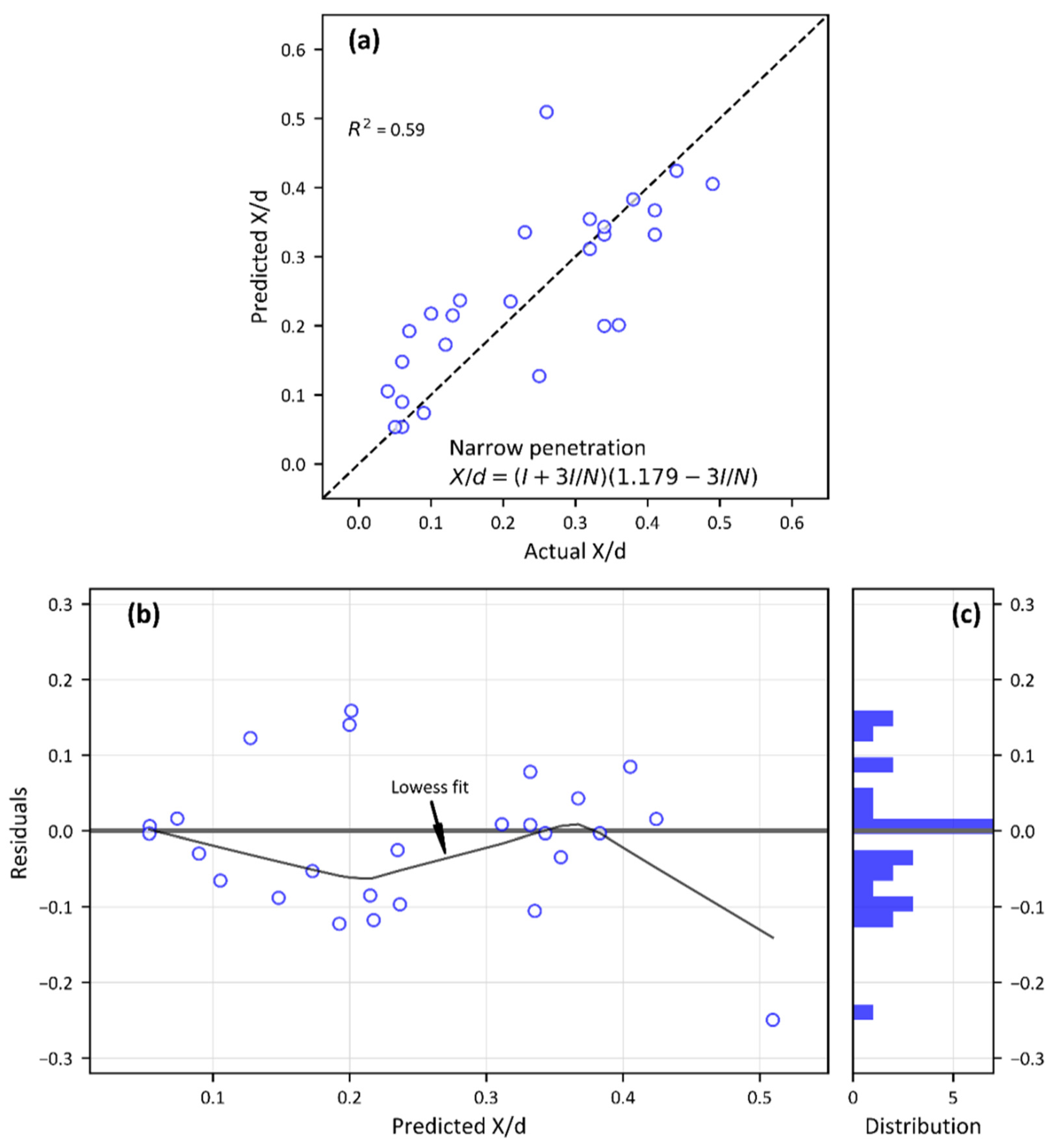
	Narrow penetration (X/d < 0.5)
R2	−3.262	0.145	−0.031	0.590
MSE	0.085	0.017	0.021	0.008
MAE	0.270	0.097	0.118	0.068
	Intermediate penetration (0.5 ≤ X/d < 5)
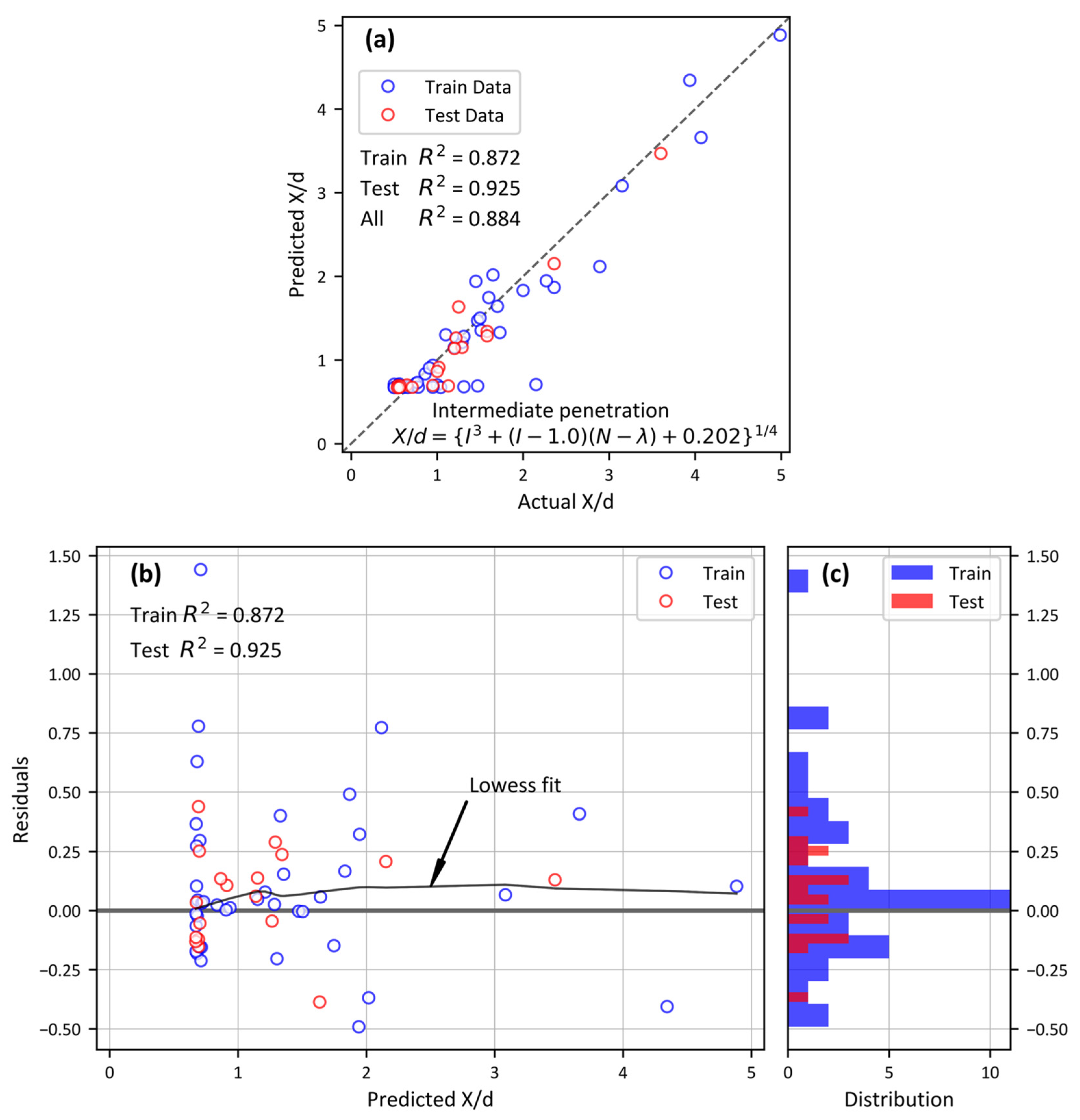
R2	0.746	0.650	0.746	0.884
MSE	0.103	0.142	0.231	0.106
MAE	0.222	0.261	0.330	0.216
	Deep penetration (X/d ≥ 5)
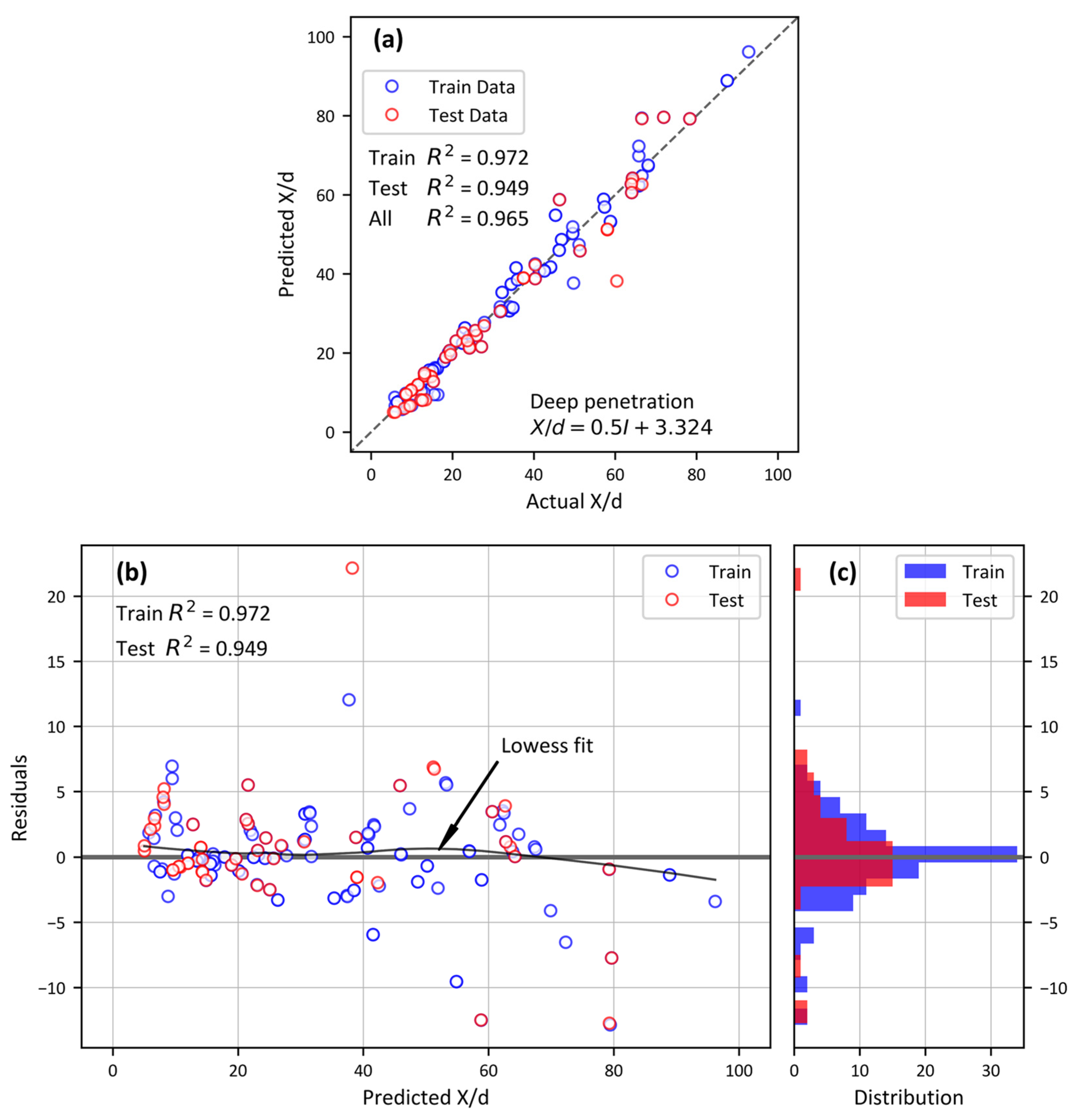
R2	0.565	-	0.963	0.967
MSE	199.369	-	16.877	15.087
MAE	11.295	-	2.799	2.470

^a Equation (1) for narrow penetration, Equation (2) for intermediate penetration, and Equation (3) for deep penetration.

for narrow, intermediate, and deep penetration, respectively. Table 4 shows the R², MSE, MAE of proposed model in comparison with NDRC, and Li and Chen model. Figure 12a shows the comparison of the model-predicted values with the actual values of narrow penetration. The coefficient of determination, R², is 0.59. Figure 12b illustrates the residual plot of predicted values. The residuals show a constant variance and are evenly spread out. The LOWESS (locally weighted scatterplot smoothing) fit is close to zero but it shows some divergence, as the variance is high at a high predicted value, which is, possibly, an outlier. The frequency distribution of residuals is shown in Figure 12c.

For the intermediate penetration data, Figure 13a compares model-predicted values with actual values. The prediction of the train and test datasets show that the model performs well on unseen test data. The coefficient of determination, R², for all data is 0.88. The residuals of predicted values are evenly distributed, as seen in the Figure 13b,c, which shows constant variance. The LOWESS fit is near zero and does not display diversion at low or high predicted values, as seen in Figure 13b.

For deep penetration data, Figure 14a compares model-predicted values with actual values. The model performs well on unseen test datasets. The coefficient of determination, R², for all data is 0.97. The residual of predicted values is evenly distributed at low or high predicted values, exhibiting a constant variance (Figure 14b,c). The LOWESS fit is close to zero, showing an absence of divergence at low or high predicted values.

Furthermore, Figure 15 shows the prediction of the proposed equation for narrow, medium, and deep penetrations compared to the Barr, NDRC, Li and Chen, and L equations. Figure 15a shows that the NDRC and Li and Chen models are almost not applicable in the narrow penetration depths. However, the present model can be useful, compared to other models with less accuracy, due to the complexity of penetration phenomena. Figure 15b,c shows that the proposed model for the prediction of X/d is more accurate, as compared to the NDRC and Li and Chen models within the range of 0.5 ≤ X/d < 5.0 and X/d ≥ 5.0.

6. Conclusions

The concrete penetration of rigid projectiles is a complex phenomenon that depends on several concrete strength parameters and projectiles. For centuries, continuous research has been conducted to predict penetration with respect to advanced tools and technology. In recent years, machine learning has evolved as an advanced statistical tool that is capable of solving complex phenomena, such as penetration, with acceptable accuracy. This research developed a new model that considers four genetic operations (crossover, sub-tree transfiguration, hoist transfiguration, and point transfiguration operations) using symbolic regression machine learning tools in Python to predict penetration and to compare with the well-established NDRC and Li and Chen models. The three equations are proposed for predicting X/d < 0.5, 0.5 ≤ X/d < 5.0, and X/d ≥ 5.0, respectively. The proposed equations show good relationships between test data and predicted X/d, with R² = 0.88 for 0.5 ≤ X/d < 5.0, and R² = 0.96 for X/d ≥ 5.0. Furthermore, the proposed model is also compared with the predictions of the NDRC and Li and Chen equations. The significance of this research shows that proposed equation predictions are more accurate than the NDRC and Li and Chen models within 0.5 ≤ X/d < 5.0 and X/d ≥ 5.0. In conclusion, it is recommended to use machine learning tools to achieve great accuracy in complex studies such as penetration, scabbing, and perforation.

References

1. Li, Q.; Reid, S.; Wen, H.; Telford, A. Local impact effects of hard missiles on concrete targets. Int. J. Impact Eng. 2005, 32, 224–284. [Google Scholar] [CrossRef]
2. Latif, Q.B.A.I.; Rahman, I.A.; Zaidi, A.M.A.; Latif, K. Critical impact energy for spalling, tunnelling and penetration of concrete slab impacted with hard projectile. KSCE J. Civ. Eng. 2014, 19, 265–273. [Google Scholar] [CrossRef]
3. Rahman, I.A.; Ahmad Zaidi, A.M.; Imran Latif, Q.B. Review on Empirical Studies of Local Impact Effects of Hard Missile on Concrete Structures. Int. J. Sustain. Constr. Eng. Technol. (IJSCET) UTHM 2010, 1, 71–95. [Google Scholar]
4. NDRC. Effects of Impact and Explosion; Summary Technical Report of Division 2; National Defence Research Committee: Washington, DC, USA, 1946; Volume 1. [Google Scholar]
5. Kennedy, R.P. A review of procedures for the analysis and design of concrete structures to resist missile impact effects. Nucl. Eng. Des. 1976, 37, 183–203. [Google Scholar] [CrossRef]
6. Haldar, A.; Hamieh, H.A. Local Effect of Solid Missiles on Concrete Structures. J. Struct. Eng. 1984, 110, 948–960. [Google Scholar] [CrossRef]
7. Hughes, G. Hard missile impact on reinforced concrete. Nucl. Eng. Des. 1984, 77, 23–35. [Google Scholar] [CrossRef]
8. Li, Q.M.; Chen, X.W. Dimensionless formulae for penetration depth of concrete target impacted by a non-deformable projectile. Int. J. Impact Eng. 2003, 28, 93–116. [Google Scholar] [CrossRef]
9. Forrestal, M.; Altman, B.; Cargile, J.; Hanchak, S. An empirical equation for penetration depth of ogive-nose projectiles into concrete targets. Int. J. Impact Eng. 1994, 15, 395–405. [Google Scholar] [CrossRef]
10. Chen, X.W.; Li, Q.M. Deep penetration of a non-deformable projectile with different geometrical characteristics. Int. J. Impact Eng. 2002, 27, 619–637. [Google Scholar] [CrossRef]
11. Milad, A.; Hussein, S.H.; Khekan, A.R.; Rashid, M.; Al-Msari, H.; Tran, T.H. Development of ensemble machine learning approaches for designing fiber-reinforced polymer composite strain prediction model. Eng. Comput. 2021, 1–13. [Google Scholar] [CrossRef]
12. Abdolrasol, M.G.M.; Hussain, S.M.S.; Ustun, T.S.; Sarker, M.R.; Hannan, M.A.; Mohamed, R.; Ali, J.A.; Mekhilef, S.; Milad, A. Artificial Neural Networks Based Optimization Techniques: A Review. Electronics 2021, 10, 2689. [Google Scholar] [CrossRef]
13. Forrestal, M.J.; Frew, D.J.; Hanchak, S.J.; Brar, N.S. Penetration of grout and concrete targets with ogive-nose steel projectiles. Int. J. Impact Eng. 1996, 18, 465–476. [Google Scholar] [CrossRef] [Green Version]
14. Frew, D.; Hanchak, S.; Green, M.; Forrestal, M. Penetration of concrete targets with ogive-nose steel rods. Int. J. Impact Eng. 1998, 21, 489–497. [Google Scholar] [CrossRef]
15. Forrestal, M.; Frew, D.; Hickerson, J.; Rohwer, T. Penetration of concrete targets with deceleration-time measurements. Int. J. Impact Eng. 2003, 28, 479–497. [Google Scholar] [CrossRef]
16. Frew, D.J.; Forrestal, M.J.; Hanchak, S.J. Penetration Experiments with Limestone Targets and Ogive-Nose Steel Projectiles. J. Appl. Mech. 2000, 67, 841–845. [Google Scholar] [CrossRef]
17. Hosseini, M.; Dalvand, A. Neural Network Approach for Estimation of Penetration Depth in Concrete Targets by Ogive-nose Steel Projectiles. Lat. Am. J. Solids Struct. 2015, 12, 492–506. [Google Scholar] [CrossRef] [Green Version]
18. Thai, D.-K.; Tu, M.; Bui, Q.; Bui, T.-T. Gradient tree boosting machine learning on predicting the failure modes of the RC panels under impact loads. Eng. Comput. 2019, 1, 3. [Google Scholar] [CrossRef]
19. Ahmad Zaidi, A.M.; Imran Latif, Q.B.; Rahman, I.A.; Ismail, M.Y. Development of empirical prediction formula for penetration of ogive nose hard missile into concrete targets with effect of CRH ratio. Am. J. Eng. Appl. Sci. 2010, 7, 711–716. [Google Scholar]
20. Duong, T.; Hazelton, M.L. Cross-validation Bandwidth Matrices for Multivariate Kernel Density Estimation. Scand. J. Stat. 2005, 32, 485–506. [Google Scholar] [CrossRef]
21. Zambom, A.Z.; Dias, R. A review of Kernel density estimation with applications to econometrics. Int. Econom. Rev. 2013, 5, 20–42. [Google Scholar]
22. Afzal, W.; Torkar, R. On the application of genetic programming for software engineering predictive modeling: A systematic review. Expert Syst. Appl. 2011, 38, 11984–11997. [Google Scholar] [CrossRef]
23. Chelapati, C.V.; Kennedy, R.P.; Wall, I.B. Probabilistic assessment of hazard for nuclear structures. Nucl. Eng. Des. 1972, 19, 333–364. [Google Scholar] [CrossRef] [Green Version]
24. Kennedy, R.P. Effects of an Aircraft Crash into a Concrete Reactor Containment Building; Holmes & Narver Inc.: Anaheim, CA, USA, 1966. [Google Scholar]
25. Bulson, P. Explosive Loading of Engineering Structures; E & FN Spon: London, UK, 1997. [Google Scholar]
26. Bangash, M.Y.H. Concrete and Concrete Structures: Numerical Modelling and Application; Elsevier Applied Science: London, UK, 1989. [Google Scholar]
27. Kar, A.K. Local Effects of Tornado-Generated Missiles. J. Struct. Div. 1978, 104, 809–816. [Google Scholar] [CrossRef]
28. Barr, P. Guidelines for the Design and Assessment of Concrete Structures Subjected to Impact; Report; UK Atomic Energy Authority, Safety and Reliability Directorate, HMSO: London, UK, 1990.
29. Kojima, I. An experimental study on local behaviour of reinforced concrete slabs to missile impact. Nucl. Eng. Des. 1991, 130, 121–132. [Google Scholar] [CrossRef]
Figure 1. Penetration of concrete caused by ogive nose rigid projectile.
Applsci 12 02040 g001
Figure 2. (a) The schematic diagrams of crossover method genetic operations. (b) The schematic diagrams of sub-tree transfiguration genetic operations. (c) The schematic diagrams of hoist transfiguration, genetic operations. (d) The schematic diagrams of point transfiguration, genetic operations.
Applsci 12 02040 g002aApplsci 12 02040 g002b
Figure 3. Flowchart of a genetic algorithm.
Applsci 12 02040 g003
Figure 4. Correlation among N, I, S, λ, and X/d using Python.
Applsci 12 02040 g004
Figure 5. Box-and-whisker plot of N, I, S, and λ, in narrow, intermediate, and deep penetration using Python.
Applsci 12 02040 g005
Figure 6. Pair plot of N, I, and S, for narrow penetration data using Python.
Applsci 12 02040 g006
Figure 7. Pair plot of N, I, and S, for intermediate penetration data using Python.
Applsci 12 02040 g007
Figure 8. Pair plot of N, I, and S, for deep penetration data using Python.
Applsci 12 02040 g008
Figure 9. Model equation for narrow penetration, in expression tree form, identified by symbolic regression.
Applsci 12 02040 g009
Figure 10. Model equation for intermediate penetration, in expression tree form, identified by symbolic regression.
Applsci 12 02040 g010
Figure 11. Model equation for deep penetration, in expression tree form, identified by symbolic regression.
Applsci 12 02040 g011
Figure 12. Symbolic regression model for narrow penetration. (a) Comparison between actual and predicted values for all data, (b) residual plot of predicted values, and (c) frequency distribution of residuals.
Applsci 12 02040 g012
Figure 13. Symbolic regression model for intermediate penetration. (a) Comparison between actual and predicted values for train and test datasets, (b) residual plot of predicted values, and (c) frequency distribution of residuals.
Applsci 12 02040 g013
Figure 14. Symbolic regression model for deep penetration. (a) Comparison between actual and predicted values for train and test datasets, (b) residual plot of predicted values, and (c) frequency distribution of residuals.
Applsci 12 02040 g014
Figure 15. Comparison of performance with different equations for (a) narrow penetration, (b) medium penetration, and (c) deep penetration.
Applsci 12 02040 g015