1. Introduction
Radar has been extensively used in anti-collision driving safety systems because it can detect a target and estimate its range. In the future, advanced radar technology is expected to become an indispensable component of self-driving vehicles [
1,
2]. Even though many sensors such as camera lidar and ultrasound are available for automotive applications, radar presents great potential, as it can detect and track a target and provide range information regardless of lighting and weather conditions. In addition, target classification is possible by capturing radar target features.
For target classification, the radar features were investigated in diverse domains. In [
3], the range profile was studied to identify target kinds. One of the most commonly used domains for the classification was the range-Doppler domain [
4,
5,
6]. In those studies, the signatures in the range-Doppler were captured and classified by deep learning algorithms. In [
7], time-varying features were considered through recurrent neural networks. Spectrogram has been extensively investigated for the classification of non-rigid body motions [
8,
9,
10]. Conversely, the development of a large array enabled the use of the point cloud model on a target for classification purposes [
11,
12]. Point clouds can provide a 3D shape of a target. However, the frontal image is based on reflection from parts of a target and has not been fully exploited.
In this paper, we investigate the feasibility of classifying targets through frontal images measured by multiple-input multiple-output (MIMO) radar. In [
13], the radar frontal image was constructed through Doppler radar by visualizing the parts of a target that are moving. This study employed MIMO radar to emulate a large array using the concept of a virtual array [
14,
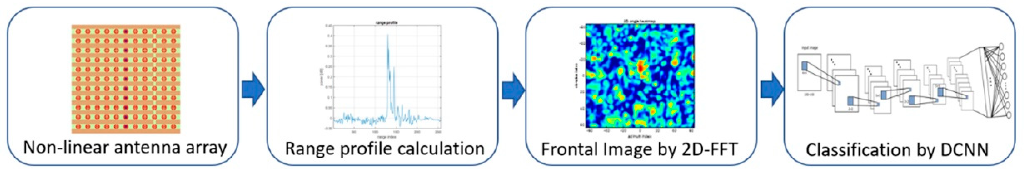
15]. The constructed array has a narrow beam width, so the reflection from each part of a target can produce a frontal image by scanning the beam. Therefore, we propose using the frontal image for target classification purposes. The frontal image can include critical information such as the physical shape of a target as well as its reflection characteristics, which can serve as a feature for target classification. The originality of this approach is that the target classification is performed using 2D frontal images rather than other radar images that have been used before such as range-Doppler diagrams and spectrograms. As the frontal image is information in a new domain that provides the continuous reflection information of all parts of the target, the reflection distribution depending on the target part becomes target features for classification. On the other hand, the point cloud model was based on 3D spatial information in locations of the strong scattering points of a target, which is discrete information. We employ deep convolutional neural networks (DCNN) to classify the radar frontal images. The general diagram of processing is shown in
Figure 1. In this paper, the concept of radar frontal image, radar signal processing, measurement campaign, DCNN structure, and results are presented.
2. Radar Frontal Image
When a 2D array is available, the direction of arrival (DOA) of the scatterer can be found in terms of the azimuth and elevation. The analytical form of the received signal of a phase array is an exponential function, of which the frequency represents the DOA. From the matched filter concept, the pseudo spectrum used to find DOA is, in general, produced by the Fourier transformation of the received signal from the array. When the pseudo spectrum is generated in 2D, it becomes the frontal image. When the received signals from an array are available, the weighted sum of the received signals reaches its maximum, which is also when the weight has the best correlation with the measure, according to the matched filter theory [
16]. The weighted sum of the received signals,
y(
k), becomes,
where
k is the sample number. Then the power of
y(
k) can be calculated as
where
is the autocorrelation matrix. When the incident wave is from
direction, the power becomes
where
is received power and
is noise power. The above equation reaches its maximum when the weight factors match the steering vector. Under that condition, the received power is
A pseudo spectrum can be constructed by changing theta and phi. In other words, the 2D Fourier transform constructs the frontal imagery that reflects the received powers from each part of a target depending on the azimuth and elevation angle. Frontal imagery pertains to the information about the physical characteristics of a target, which is critical in target classification.
To construct the data set, we use a millimeter-wave FMCW radar system developed by Smart Radar Systems. The radar system comprises four AWR1243 chips (from TI Co. Ltd., Gumi-si, Korea) operating at 77 GHz with 12 dBm of transmitting power. Each AWR1243 has three TXs and four RXs, thus allowing the construction of a 16 virtual Rx array for each chip. Cascading four chips makes 192 channels available through 12 TXs and 16 RXs. The radar employs a sparse antenna array for DOA estimation with improved angular resolution [
14]. Using a non-linear MIMO antenna configuration, the radar antenna produced a 2D virtual array of 31 × 33, resulting in an angular resolution of approximately 3.5 degrees for the azimuth and elevation.
3. Target Measurements
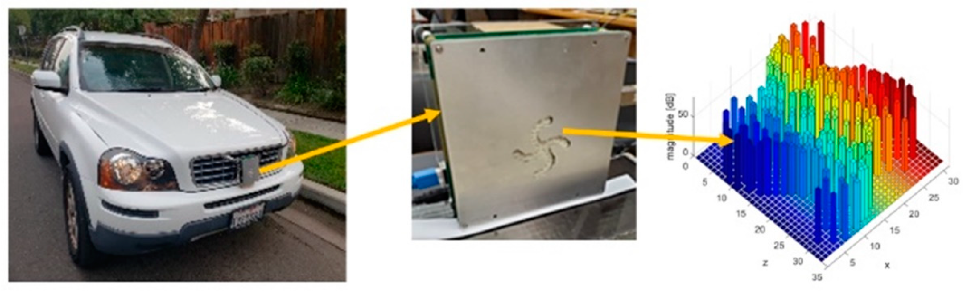
We installed the MIMO radar system in front of a car and measured five targets. The radar was located in the middle of the bumper at a height of 75 cm, as shown in
Figure 2. The physical shape of the MIMO radar is also shown in the figure. The target types include sedans, SUVs, trucks, trees, poles, and humans. For each class, we measured 50 different objects.
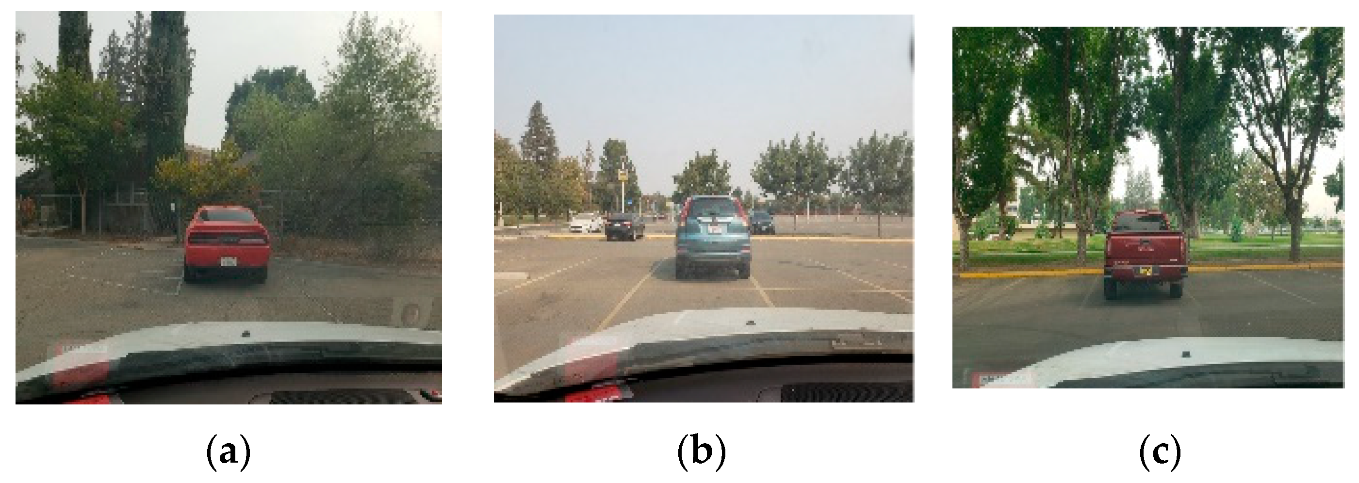
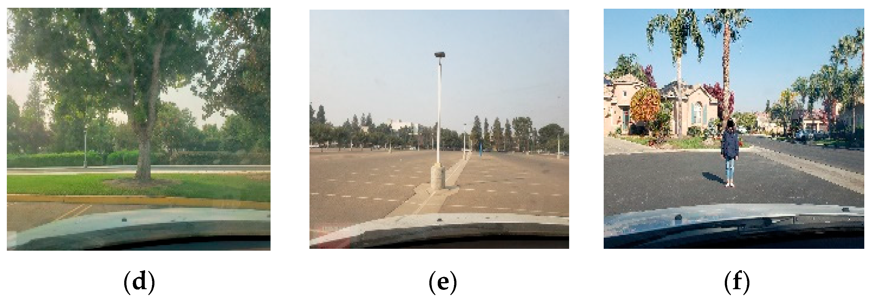
The measurement campaigns are presented in
Figure 3. During the measurement, the platform vehicle was slowly moving at under 5 m/h. The target was measured in the range between 1 m and 12 m because the target can be well visualized when it is close to the radar. The target vehicles were measured in the street and in parking lots. For clutter such as trees and poles, we measured them while the platform vehicle moved slowly. Human subjects were measured while both the subject and the platform were moving.
4. Radar Signal Processing
The parameters of the FMCW radar were set as follows. The number of chirps per frame was 64, the frame period was 200 msec, and the total measurement duration was 5 s, resulting in total chirps recorded of 64 × 25 = 1600 for each target measurement. Each chirp produced a target frontal image. However, we extracted only 2 chirps randomly per frame because the images are very similar within the frame, as the time duration is only a couple of microseconds. Therefore, the total extracted images per target kind were 2 × 25 × 50 = 2500.
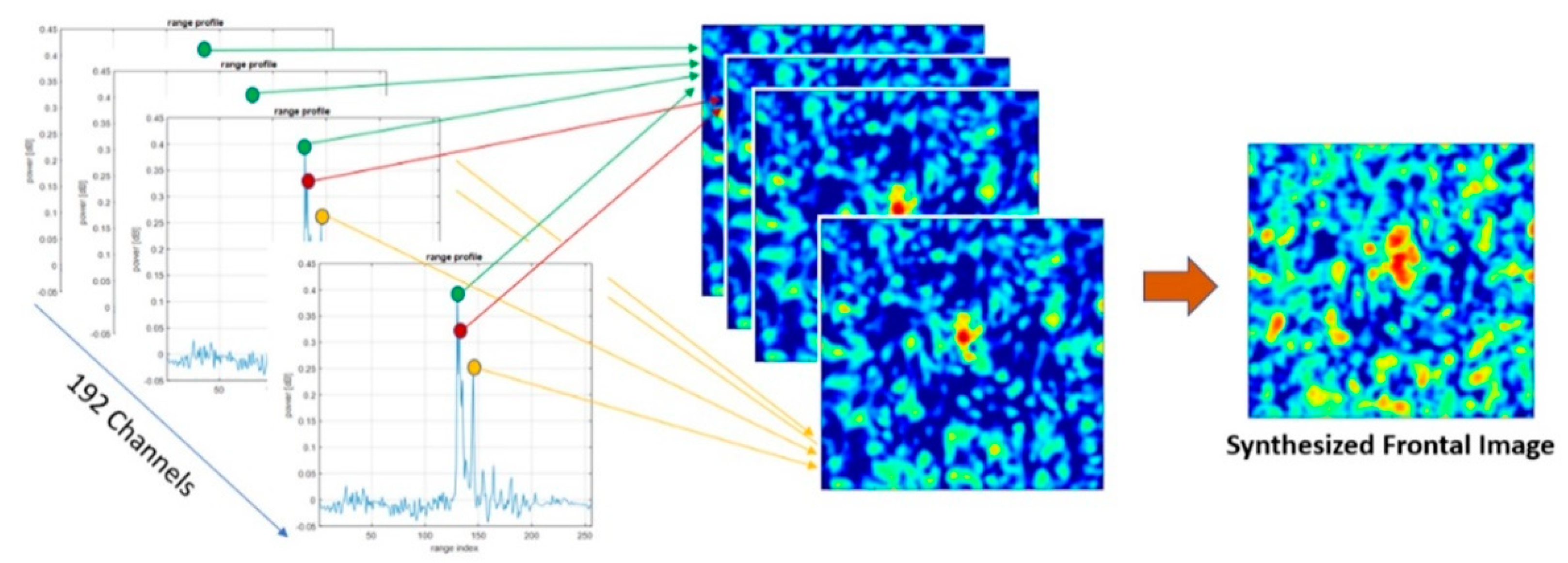
The received FMCW signals were processed to construct the radar frontal images. The physical 192 channels are distributed to have a nonlinear array as shown in
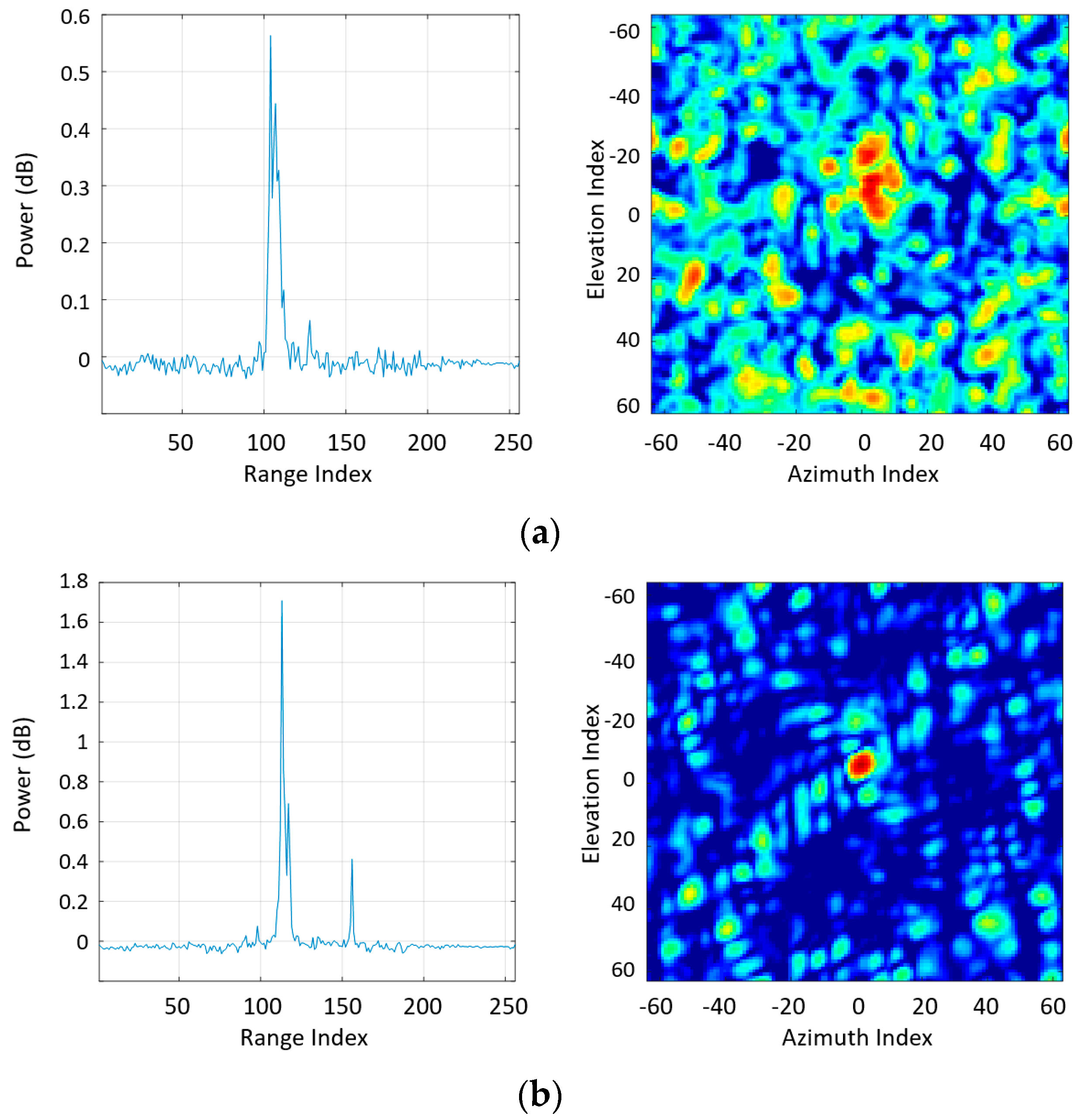
Figure 2. As channels exist in 31 × 33 dimensions, a total of 1023 (31 × 33) virtual receiving channels were regarded to have their own down-converted signals in the time domain. The time-domain signal was transformed to the frequency domain through Fourier transformation, which serves as a range profile as presented in
Figure 4 as an example. In the range profile, a target is detected based on the simple threshold method. However, as the target occupies several bins in the range profile, the determination of the threshold is critical as it affects the quality of the radar frontal image. The complex value (phasor) of the individual point detected in the range profile from each channel was extracted and 2-dimensional Fourier-transformed was executed to construct the frontal image. Accordingly, when there are multiple points detected in the range profile, the total image should be synthesized by overlapping several frontal images. This process is demonstrated in
Figure 4.
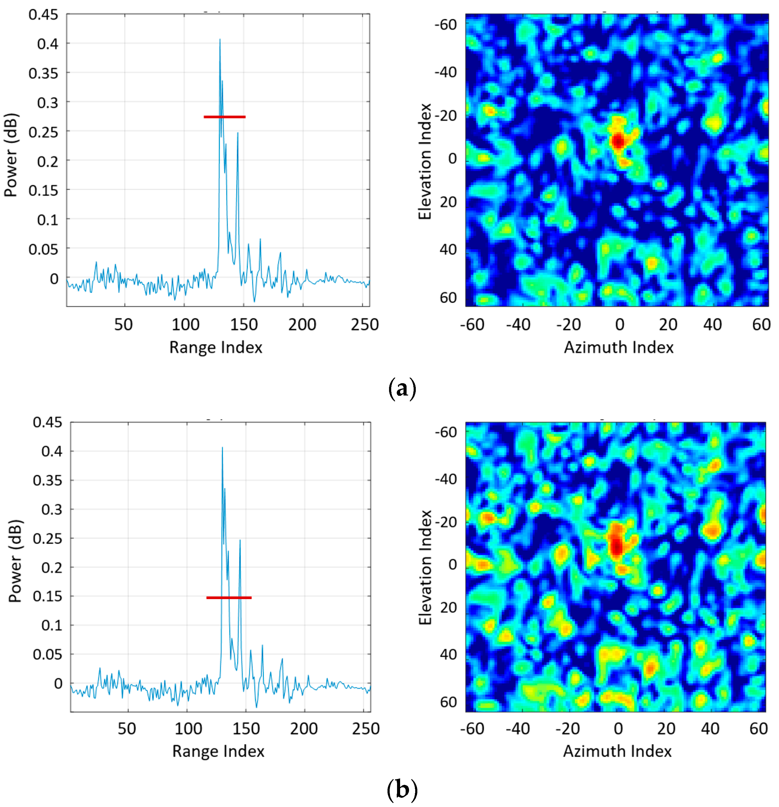
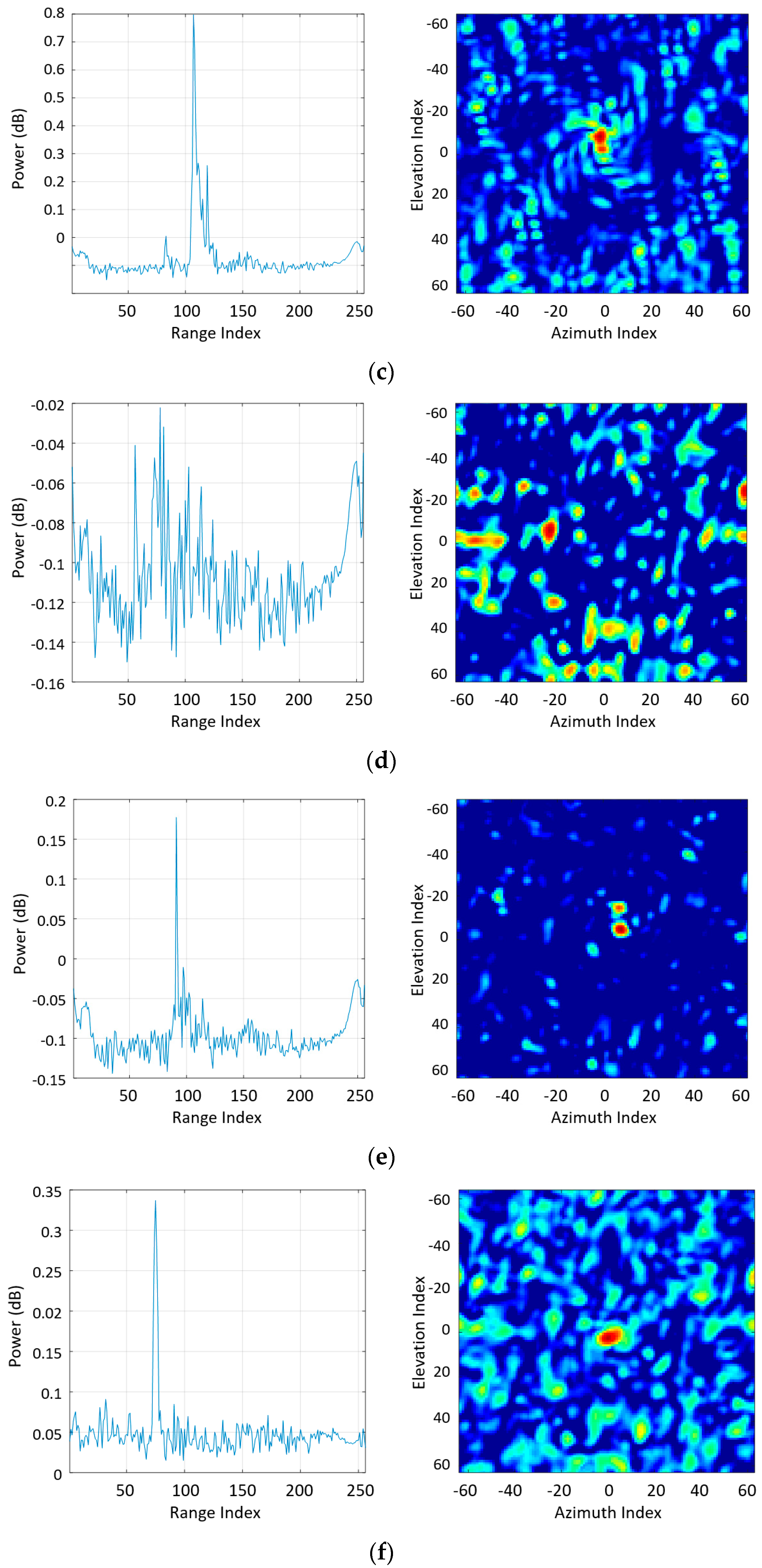
When the threshold is too high, very few points will contribute to producing the image, as in
Figure 5a. In this case, the threshold was 3/5 of the peak. As the threshold decreases, many points in the range profile contribute to a single frontal image, which can cause noise issues. The impact on the low threshold is presented in
Figure 5b. The figure indicates that several points should be involved in the construction of a target’s detailed characteristics. We heuristically set the threshold at a 1/3 of the peak because it provides reasonable characteristics for frontal images. The measured frontal images for each target are presented in
Figure 6.
5. Deep Convolutional Neural Networks
We have two scenarios for target classification based on radar frontal images. First, we classified six classes using a DCNN. The six classes were sedan, van, truck, pole, tree, and human. In the second scenario, we classified 3 classes, vehicles (sedan, van, truck), humans, and clutter (pole and tree). To classify targets, we used deep neural networks that surpass previous classifiers, as they are proven to be excellent at abstraction and generalization for radar target classification [
17,
18,
19,
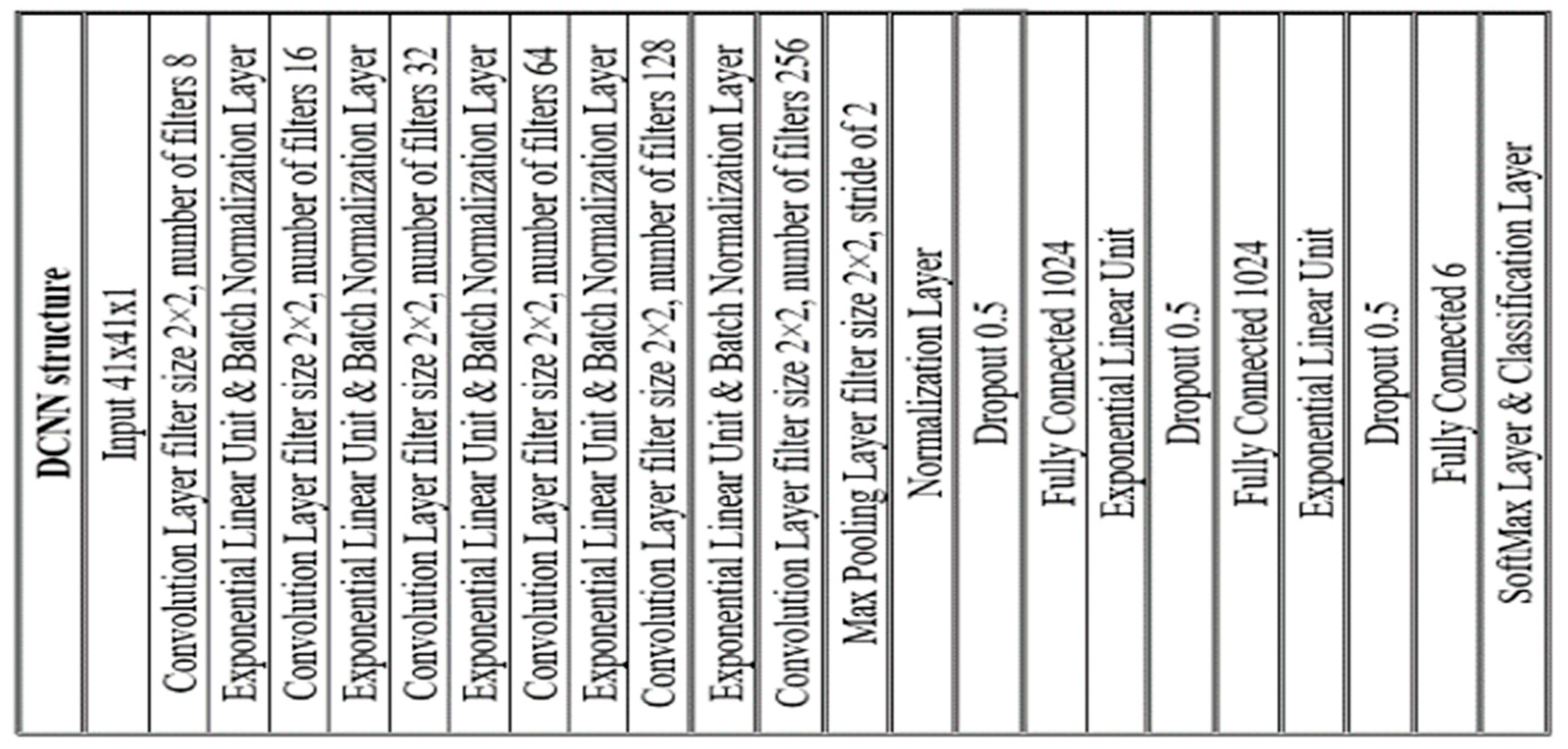
20]. The DCNN extracts images feature through the convolution of those images which leads to high performance in target recognition. In this paper, road target detection and classification method based on DCNN is suggested. A DCNN is mainly consisting of multiple convolution layers, pooling layers, and fully connected layers, and finally uses SoftMax to classify and output. This architecture on the types and numbers of layers is varied depending on the size and characteristics of the dataset. Convolutional layers are the first layers of the DCNN architecture, which extract features of images through convolutional filters. The layers located between each of the two convolutions layers are pooling layers that are responsible for simplifying the data by reducing its dimensionality. This minimizes the time required for training and helps to restrain the problem of overfitting. The last layers of the deep learning network are the fully connected layers. In these layers, every neuron in the first is connected to every neuron in the next. The process during this network training looks at what features most accurately describe the specific classes, and the output generates the probabilities that are organized according to each class. For each objective, a DCNN structure was optimized heuristically. The structure of DCNN is divided into three main parts. The first part passes the input into a set of convolution layers with a filter size of 2 × 2 and then into the max-pooling layer. The second part is the same as the first except for the increased number of filters in the convolution layers with the max-pooling layer at the end. The last part is fully connected layers with dropout layers. In the fully connected layer, each neuron is connected to all neurons in the previous layer. The ReLu layer is applied after every convolutional and fully connected layer to not activate all the neurons at the same time. Since only a certain number of neurons are activated, the ReLu function is computationally efficient. The dropout layer is applied before the first and the second are fully connected to reduce overfitting and improve the generalization of deep neural networks. The designed network is presented in
Figure 7.
Although the measurements are conducted in a controlled environment, some data are quite noisy due to the low SNR. For example, measured data from targets such as poles, trees, and humans could not be fully used for training when images become very noisy. Thus, the class with the smallest data samples becomes the reference. Finally, each class has 2047 data points; a total of 10,235 radar images are available for training. For the construction of the data set, we cropped the frontal image to a size of 40 × 40 pixels, with the peak power in the center. We also normalized the image values from 0 to 255.
The data are divided into a training set (80%), a testing set (10%), and a validation set (10%). For the training, the stochastic gradient descent with momentum optimizer was used with an initial learning rate of 0.0004 and a momentum of 0.9. To improve the training, the training loss is dropped every ten epochs using exponential decay with a decay rate of 0.96. The mini-batch size was set to 32, and the max epoch was set at 1000. To prevent overfitting, an early stop was set to monitor the validation loss and stop after five epochs if the losses were not dropping, at which point training stops. We used a five-fold validation method by shuffling the dataset. As seen in
Table 1, the classification accuracy for 6 classes yielded 87.1%. The confusion matrix is shown in
Table 2. If we want to classify only 3 classes such as vehicles, humans, and clutter, then the accuracy is 92.6%.
6. Conclusions
In this study, we investigated the feasibility of classifying targets through frontal imaging. Rather than exploring signatures in the range profile, range-Doppler or spectrogram domain, the frontal images constructed along with azimuth and elevation served as key a feature in the classification process. In the synthesis of the frontal image, several frontal images corresponding to each bin in the range profile are overlapped. DCNN was exploited as a classifier and was trained by the stochastic gradient descent with a momentum optimizer. The confusion matrix revealed that the classification accuracy for sedans, SUVs, trucks, trees, poles, and humans yielded up to 87.1%. If the classifier was designed to classify vehicles, humans, and clutter, the classification rate increases to 92.6%. However, it should be noted that the classification accuracy using the proposed method is not higher than that of other methods such as the use of the range-Doppler domain. The results showed that the frontal image can potentially serve as one of the modalities in the target classification scheme, yet high spatial-resolution radar should be developed, or other features can also be incorporated together to maximize performance.
Author Contributions
Conceptualization, Y.K., S.Y. and B.J.J.; methodology, Y.K. and S.Y.; software, M.E.; validation, M.E. and B.J.J.; formal analysis, M.E.; writing—original draft preparation, M.E. and Y.K.; writing—review and editing, Y.K. and S.Y.; visualization, M.E.; supervision, S.Y. and B.J.J.; project administration, S.Y. and B.J.J.; funding acquisition, S.Y. and B.J.J. All authors have read and agreed to the published version of the manuscript.
Funding
This work was supported by an Electronics and Telecommunications Research Institute (ETRI) grant funded by the Korean government [22ZH1100, Study on 3D Communication Technology for Hyperconnectivity] and the National Research Foundation (NRF), Korea [BK21 FOUR].
Institutional Review Board Statement
The study was conducted in accordance with the Declaration of Helsinki and approved by the Institutional Review Board of California State University, Fresno.
Informed Consent Statement
Informed consent was obtained from all subjects involved in the study. Written informed consent was obtained from the subjects to the publication of this paper.
Data Availability Statement
Not applicable.
Conflicts of Interest
The authors declare no conflict of interest.
References
- Hasch, J.; Topak, E.; Schnabel, R.; Zwick, T.; Weigel, R.; Waldschmidt, C. Millimeter-wave technology for automotive radar sensors in the 77 GHz frequency band. IEEE Trans. Microw. Theory Tech. 2012, 60, 845–860. [Google Scholar] [CrossRef]
- Fan, Y.; Xiang, K.; An, J.; Bu, X. A new method of multi-target detection for FMCW automotive radar. In Proceedings of the IET International Radar Conference 2013, Xi’an, China, 14–16 April 2013. [Google Scholar]
- Liu, J.; Xu, Q. Radar target classification based on high resolution range profile segmentation and ensemble classification. IEEE Sens. Lett. 2021, 5. [Google Scholar] [CrossRef]
- Wit, J.; Dorp, P.; Huizing, A. Classification of air targets based on range-Doppler diagrams. In Proceedings of the European Radar Conference (EuRAD), London, UK, 5–7 October 2016. [Google Scholar]
- Ng, W.; Wang, G.; Siddhartha; Lin, Z.; Dutta, B. Range-Doppler detection in automotive radar with deep learning. In Proceedings of the International Joint Conference on Neural Networks (IJCNN), Glasgow, UK, 19–24 July 2020.
- Tan, K.; Yin, T.; Ruan, H.; Balon, S.; Chen, X. Learning approach to FMCW radar target classification with feature extraction from wave physics. IEEE Trans. Antennas Propag. 2022, 70, 6287–6299. [Google Scholar] [CrossRef]
- Kim, Y.; Alnujaim, I.; You, S.; Jeong, B. Human detection based on time-varying signature on range-Doppler diagram using deep neural networks. IEEE Geosci. Remote Sens. 2021, 18, 426–430. [Google Scholar] [CrossRef]
- Padar, M.; Ertan, A.; Candan, C. Classification of human motion using radar micro-Doppler signatures with hidden Markov models. In Proceedings of the 2016 IEEE Radar Conference (RadarConf), Philadelphia, PA, USA, 2–6 May 2016. [Google Scholar]
- Jokanovic, B.; Amin, M.; Ahmad, F. Radar fall motion detection using deep learning. In Proceedings of the 2016 IEEE Radar Conference (RadarConf), Philadelphia, PA, USA, 2–6 May 2016; pp. 1–6. [Google Scholar]
- Amin, M.; Ahmad, F.; Zhang, Y.; Boashash, B. Human gait recognition with cane assistive device using quadratic time–frequency distributions. IET Radar Sonar Navigat. 2015, 9, 1224–1230. [Google Scholar] [CrossRef] [Green Version]
- Feng, Z.; Zhang, S.; Kunert, M.; Wiesbeck, W. Point cloud segmentation with a high-resolution automotive radar. In Proceedings of the AmE 2019—Automotive meets Electronics; 10th GMM-Symposium, Dortmund, Germany, 12–13 March 2019. [Google Scholar]
- Sengupta, A.; Cao, S.; Wu, Y. MmWave radar point cloud segmentation using GMM in multimodal traffic monitoring. In Proceedings of the International Radar Conference (RADAR), Florence, Italy, 28–30 April 2020. [Google Scholar]
- Lin, A.; Ling, H. Frontal imaging of human using three-element Doppler and direction-of-arrival radar. Electron. Lett. 2006, 42, 660–661. [Google Scholar] [CrossRef]
- Tan, Z.; Nehorai, A. Sparse direction of arrival estimation using co-prime arrays with off-grid targets. IEEE Signal Process. Lett. 2014, 21, 26–29. [Google Scholar] [CrossRef]
- Duan, G.; Wang, D.; Ma, X.; Su, Y. Three-dimensional imaging via wideband MIMO radar system. IEEE Geosci. Remote Sens. Lett. 2010, 7, 445–449. [Google Scholar] [CrossRef]
- Chen, Z.; Gokeda, G. Introduction to Direction-of-Arrival Estimation; Artech House: Norwood, MA, USA, 2010. [Google Scholar]
- Kim, Y.; Moon, T. Human detection and activity classification based on micro-Dopplers using deep convolutional neural networks. IEEE Geosci. Remote Sens. Lett. 2016, 13, 2–8. [Google Scholar] [CrossRef]
- Seyfioğlu, M.; Özbayoğlu, A.; Gürbüz, S. Deep convolutional autoencoder for radar-based classification of similar aided and unaided human activities. IEEE Trans. Aerosp. Electron. Syst. 2018, 54, 1709–1723. [Google Scholar] [CrossRef]
- Patel, K.; Rambach, K.; Visentin, T.; Rusev, D.; Pfeiffer, M.; Yang, B. Deep Learning-based Object Classification on Automotive Radar Spectra. In Proceedings of the 2019 IEEE Radar Conference (RadarConf), Boston, MA, USA, 22–26 April 2019. [Google Scholar]
- Neumann, C.; Brosch, T. Deep learning approach for radar applications. In Proceedings of the 2020 21st International Radar Symposium (IRS), Warsaw, Poland, 5–8 October 2020. [Google Scholar]
| Publisher’s Note: MDPI stays neutral with regard to jurisdictional claims in published maps and institutional affiliations. |
© 2022 by the authors. Licensee MDPI, Basel, Switzerland. This article is an open access article distributed under the terms and conditions of the Creative Commons Attribution (CC BY) license (https://creativecommons.org/licenses/by/4.0/).


