Article

Dual Band Antenna Design and Prediction of Resonance Frequency Using Machine Learning Approaches

1
Department of Electrical and Electronic Engineering, Universiti Teknologi PETRONAS, Bandar Seri Iskandar 32610, Perak, Malaysia
2
Department of Electrical and Electronic Engineering, Daffodil International University, Dhaka 1341, Bangladesh
3
Department of Electrical and Electronic Engineering, Jatiya Kabi Kazi Nazrul Islam University, Mymensingh 2220, Bangladesh
4
Faculty of Data Science and Information Technology, INTI International University, Persiaran Perdana BBN, Putra Nilai, Nilai 71800, Negeri Sembilan, Malaysia
5
Department of Computer Science and Engineering, Daffodil International University, Dhaka 1341, Bangladesh
6
Department of Electrical, Electronic and Communication Engineering, Pabna University of Science and Technology, Pabna 6600, Bangladesh
7
Condition Monitoring Systems Lab, NCRA, Mehran University of Engineering and Technology, Jamshoro 67480, Pakistan
8
Department of Computer Science and Engineering, City University, Dhaka 1343, Bangladesh
*
Author to whom correspondence should be addressed.
Appl. Sci. 2022, 12(20), 10505; https://doi.org/10.3390/app122010505
Submission received: 2 September 2022 / Revised: 28 September 2022 / Accepted: 4 October 2022 / Published: 18 October 2022

Abstract

:
An inset fed-microstrip patch antenna (MPA) with a partial ground structure is constructed and evaluated in this paper. This article covers how to evaluate the performance of the designed antenna by using a combination of simulation, measurement, creation of the RLC equivalent circuit model, and the implementation of machine learning approaches. The MPA’s measured frequency range is 7.9–14.6 GHz, while its simulated frequency range is 8.35–14.25 GHz in CST microwave studio (CST MWS) 2018. The measured and simulated bandwidths are 6.7 GHz and 5.9 GHz, respectively. The antenna substrate is composed of FR-4 Epoxy, which has a dielectric constant of 4.4 and a loss tangent of 0.02. The equivalent model of the proposed MPA is developed by using an advanced design system (ADS) to compare the resonance frequencies obtained by using CST. In addition, the measured return loss of the prototype is compared with the simulated return loss observed by using CST and ADS. At the end, 86 data samples are gathered through the simulation by using CST MWS, and seven machine learning (ML) approaches, such as convolutional neural network (CNN), linear regression (LR), random forest regression (RFR), decision tree regression (DTR), lasso regression, ridge regression, and extreme gradient boosting (XGB) regression, are applied to estimate the resonant frequency of the patch antenna. The performance of the seven ML models is evaluated based on mean square error (MSE), mean absolute error (MAE), root mean square error (RMSE), and variance score. Among the seven ML models, the prediction result of DTR (MSE = 0.71%, MAE = 5.63%, RMSE = 8.42%, and var score = 99.68%) is superior to other ML models. In conclusion, the proposed antenna is a strong contender for operating at the entire X-band and lower portion of the Ku-band frequencies, as evidenced by the simulation results through CST and ADS, it measured and predicted results using machine learning approaches.

1. Introduction

Antennas are rightfully referred to as the electronic eyes and ears of the planet because of their unquestionable significance in wireless communication technology [1]. Microstrip patch antennas (MPAs) have been one of the most revolutionary breakthroughs in the time of downsizing in the ever-growing field of wireless communication technology [2,3]. Due to their low weight, miniature size, affordability, ease of fabrication, and ability to be printed directly onto circuit boards, they have been widely used in various wireless systems, such as airborne radar, radio telemetry, RFID, mobile communication, navigation systems, and satellite communication [4,5]. In [6,7], meta surface-based dual band antennas were investigated, especially for industrial, scientific, and medical (ISM) applications. When the incident angles theta and phi change from −90 to 90 and from 0 to 360 degrees, the unit “1” reflection coefficient amplitude changes from 0 to 1. A genetic algorithm (GA) optimizes CFMS coding subarray distribution [6]. The S11 of the antenna is less than −10 dB between 2.3–2.62 GHz and 4.9–6.45 GHz and 13% and 27% impedance bandwidth. Additionally, 6.8 dB at 2.45 GHz and 9.0 dB at 5.8 GHz [7]. However, the bandwidth and gain of typical microstrip antennas are both low [8,9], despite their many advantages. Recently, MPAs have been extensively used in X-band applications. An X-band antenna can have both the compact size and the huge bandwidth required to send big data [10,11]. To increase MPA performance and eliminate numerous drawbacks in the X-band range, substantial research work was conducted accordingly [12,13,14,15,16,17]. A tuning fork-shaped MPA having resonance frequencies ranging from 9 GHz to 11 GHz for X-band radar and satellite applications was presented in [18]. The substrate of Rogers RT/Duroid 5880 in a high-frequency structural simulator (HFSS) simulates and analyzes the antenna characteristics. With total dimensions of 24 × 18 × 1.57 mm3, the result generated a maximum gain of 5.3 dB. A series-fed microstrip array antenna was also proposed in [19] for X-band applications by using an array structure with a dimension of 156 × 9 mm2. In [20], a 3D printed corrugated plate antenna with high gain and aperture efficiency was proposed in the work. It is reported that the gain of the antenna is improved with the increment of the number of corrugated structures. The highest gain of 24.2 dB was achieved when 10 corrugations were implemented in the antenna structure. A proximity coupled technique is also being proposed for microstrip patch antennas (PC-MSPA) in S/C/X-band applications as reported in [21]. The prediction of the impedance response was conducted for a two-layer and single-material design structure. As a result, a new prediction model based on an electric equivalent circuit was introduced accordingly. To achieve the acceptable performance of an antenna using 3D electromagnetic simulation software, such as CST, HFSS, FEKO, and ADS, is a very challenging and time-consuming task. To mitigate these limitations, many researchers apply machine learning (ML) and deep learning (DL) approaches to optimize the antenna design, predict the results, such as resonance frequency ( f r ), gain, return loss (s11), bandwidth, and so on, and select the antennas for wireless applications [22,23,24,25,26,27,28,29]. Authors in [30] proposed an artificial neural network (ANN)-based microstrip patch antenna where the antenna dimension and resonance frequencies were predicted. However, the accuracy of the predicted results in terms of percentage of error, such as MSE, MAE, and RMSE, was not considered. Moreover, the prediction results of the proposed ANN model were not compared with the other existing ML models to validate the prediction. Another research work was carried out to predict the resonance frequency of patch antennas using ANN in [31]. In this research work, the percentage of error was calculated from the difference between actual value and predicted value divided by the actual value. It is noteworthy that the percentage of error in terms of MSE, MAE, and RMSE was not evaluated. In addition, most of the existing ML-based antenna design research work has not measured the variance score. In this research work, six regression ML models, such as linear regression (LR), random forest regression (RFR), decision tree regression (DTR), Lasso regression, ridge regression (RR), extreme gradient boosting (XGB) regression, and one DL model (CNN), are used to predict the operating frequency of the proposed antenna. Various performance metrics, such as mean square error (MSE), mean absolute error (MAE), root MSE (RMSE), and variance score are observed to validate the prediction of the f r using the mentioned models [32].
Recently, a new technique has been explored by using multiple regression algorithms along with convolutional neural networks (CNN) to predict the f r by using CST electromagnetic (EM) simulation tools. Furthermore, the simulated f r using CST and ADS and measured f r is compared with the predicted f r using the proposed ML algorithms.
The main contributions of this research work are summarized as follows:
i
Simulate and analyze the performance of a microstrip patch antenna using CST EM simulation tools.
ii
Validate the CST simulation results using ADS simulation software, and the simulated S11 is compared with the measured S11.
iii
The resonance frequency ( f r ) is predicted using six ML regression algorithms and CNN. A comparative study of the different models based on the different predicted results is incorporated.
The remaining sections of this study are organized as follows. Section 2 explains several generic design formulas and the geometrical structure of the proposed antenna and the required performance analysis of the various machine learning algorithms. The results of the necessary simulations and measurements are presented in Section 3 and, consequently, the concluding remarks are highlighted in Section 4.

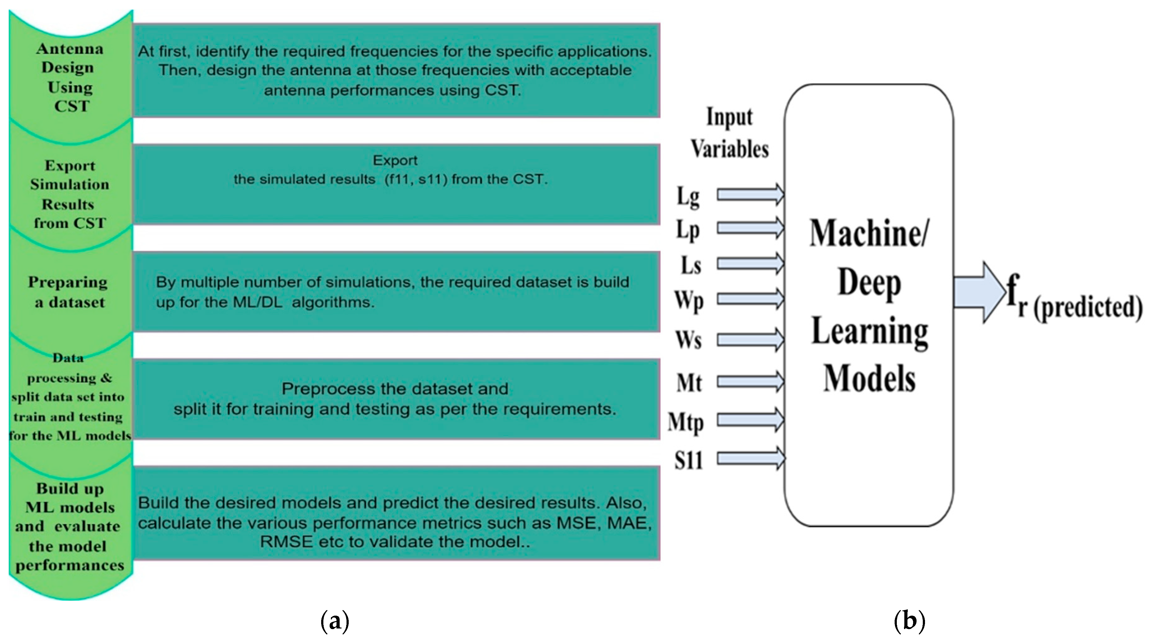
2. Design Methodology

In microstrip patch antennas, the size and shape of the patch determine the antenna’s resonance frequency, bandwidth, return loss, gain, and radiation pattern. Radiation efficiency and resonance frequency are two of the many variables whose values are directly determined by the patch’s width and length. The feasible and efficient dimensions (length and width) of a rectangular microstrip antenna can be calculated using the formulae below. Based on the transmission line model, the dimensions of a radiation patch can be calculated using the following equations [33,34]:
W = c 2 f r 2 ϵ r + 1
L = c 2 f r ϵ e f f + 1 2 Δ L
where
Δ L = 0.412 h ϵ e f f + 0.3 ϵ e f f 0.258 w h + 0.264 w h + 0.8
ϵ e f f = ϵ r + 1 2 + ϵ r 1 2 1 + 12 h w 1 2
and feedline W0 is evaluated from the input impedance Zin:
Z i n = 120 π ϵ r h w + 1.393 + 0.667 l n h w + 1.444
Here, c is the speed at which light travels through a vacuum, ( f r ) is the resonance frequency, and ε r is the relative permittivity (also called the dielectric constant) of the dielectric material. In real life, the fields do not just stay on the patch. The fringing field is a field component that goes beyond the patch’s physical limits (L × W). The effective patch width could be calculated using the effective dielectric constant ( ε r e f f ) for the width of the patch (W) while considering the influence of the fringing field effect. The effective dielectric constant ( ε r e f f ) is determined by the following equation:
ϵ e f f = ϵ r + 1 2 + ϵ r 1 2 1 + 12 h w 1 2
Here, h is the thickness of dielectric substrate. To account for the influence of the fringing field given a patch length L, both ends of the line must have a length added to them.
Δ L ϵ e f f h = 0.412 h ϵ e f f + 0.3 w h + 0.264 ϵ e f f 0.258 w h + 0.8
The antenna has a total footprint of 28.2 × 23.8 × 1.6 mm3 with a patch area of 28.2 × 23.8 mm2. Annealed copper is used as a patch and ground plane material and is matched to the real-world antenna construction material.
FR4 is, rightly, the most commonly used material in PCB construction. Boards from FR4 are robust, water resistant, and provide sound insulation between copper layers that minimize interference and support good signal integrity. This research investigated the feasibility of using the FR-4 substrate for microstrip antennas throughout a wide frequency range (8–12 GHz). The purpose of this investigation was to examine the FR-4 substrate as a potential option for designing an X-band microstrip antenna, aiming to achieve a high degree of agreement between simulated and measured results. Due to its inexpensive cost and widespread availability, FR-4 was selected for this research because it can be utilized for prototyping microstrip antennas. A microstrip feed line with a 50 Ω impedance was used to feed the input signal to the antenna. CST carries out the preliminary design and performance optimization. The dimensional parameters of the proposed MPA are presented in Table 1.
The proposed MPA utilizes FR-4 Epoxy dielectric material, which has a relative permittivity of ε r = 4.4 and loss tangent of 0.007. The antenna features a rectangle-shaped patch with two inset slot cuts and a partial ground plane with a smaller area than the substrate. The parametric analysis in CST derives the optimal dimensions of insets and ground planes. Optimized dimensions of inset slots in combination with a partial ground plane give an excellent wideband response. Figure 1a,b depict a simulated 3D view; the partial ground plane of the proposed MPA and Figure 2a shows the dimensions of substrate, patch, and feedline of the proposed X-band MPA and Figure 2b depicts the fabricated prototype view of the proposed wideband MPA that has the capability to satisfy X-band applications requirement.

3. Result Analysis of the Proposed MPA

The simulated and measured results of the proposed MPA are discussed in this section. The simulated S11 using CST is also compared with the results obtained from the advanced design system (ADS). Finally, different machine learning algorithms are discussed briefly to predict the proposed antenna’s resonance frequency.

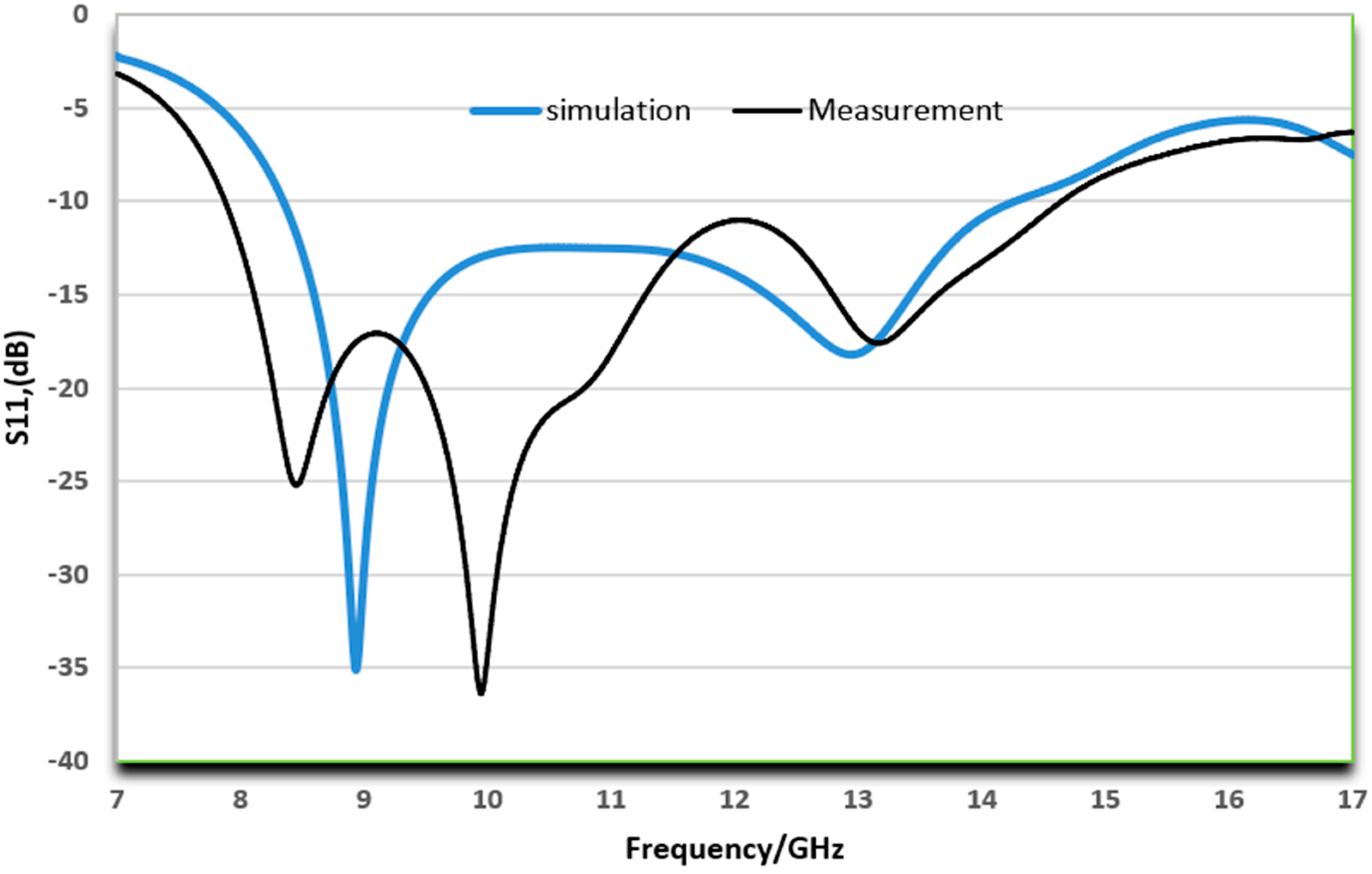
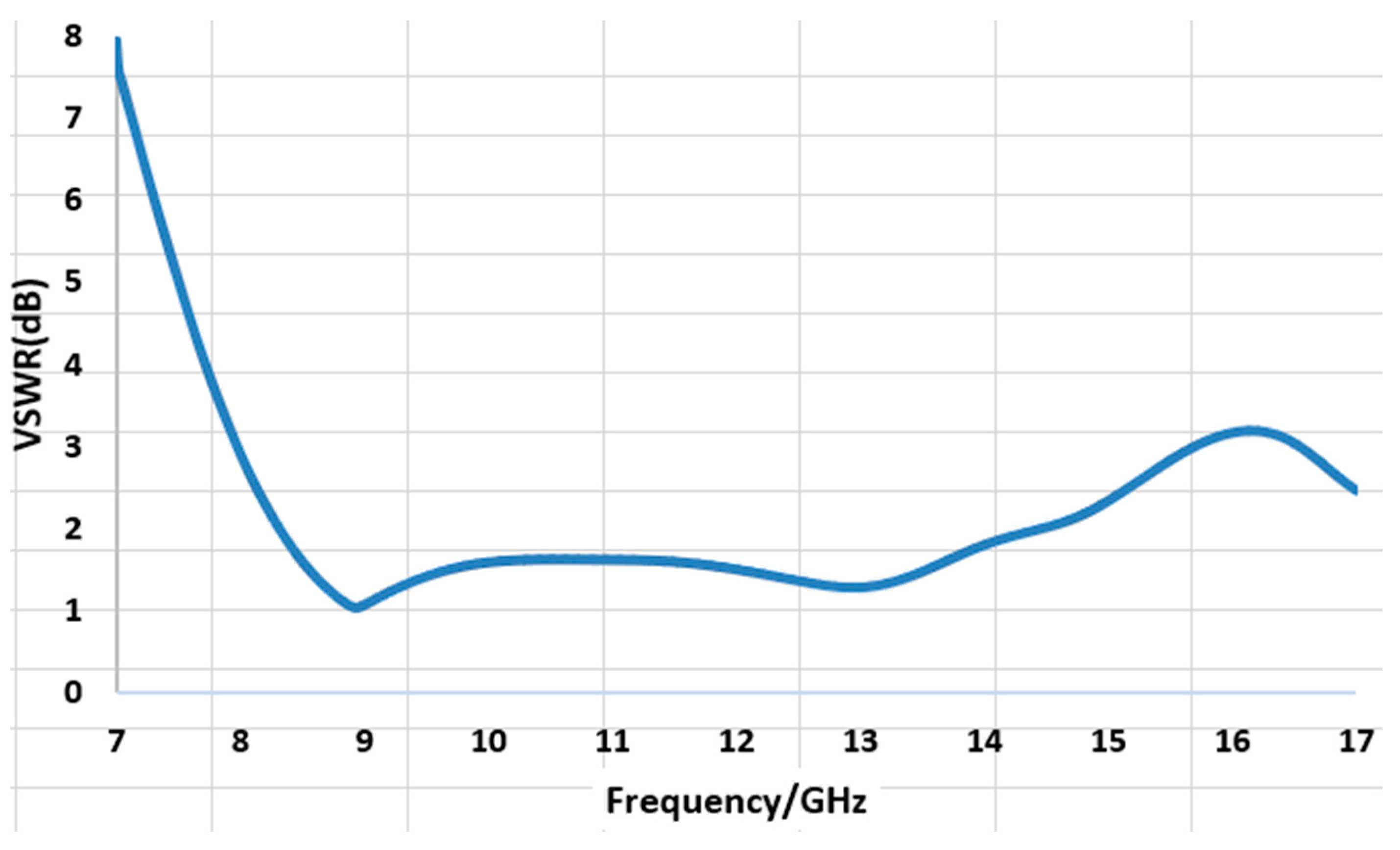
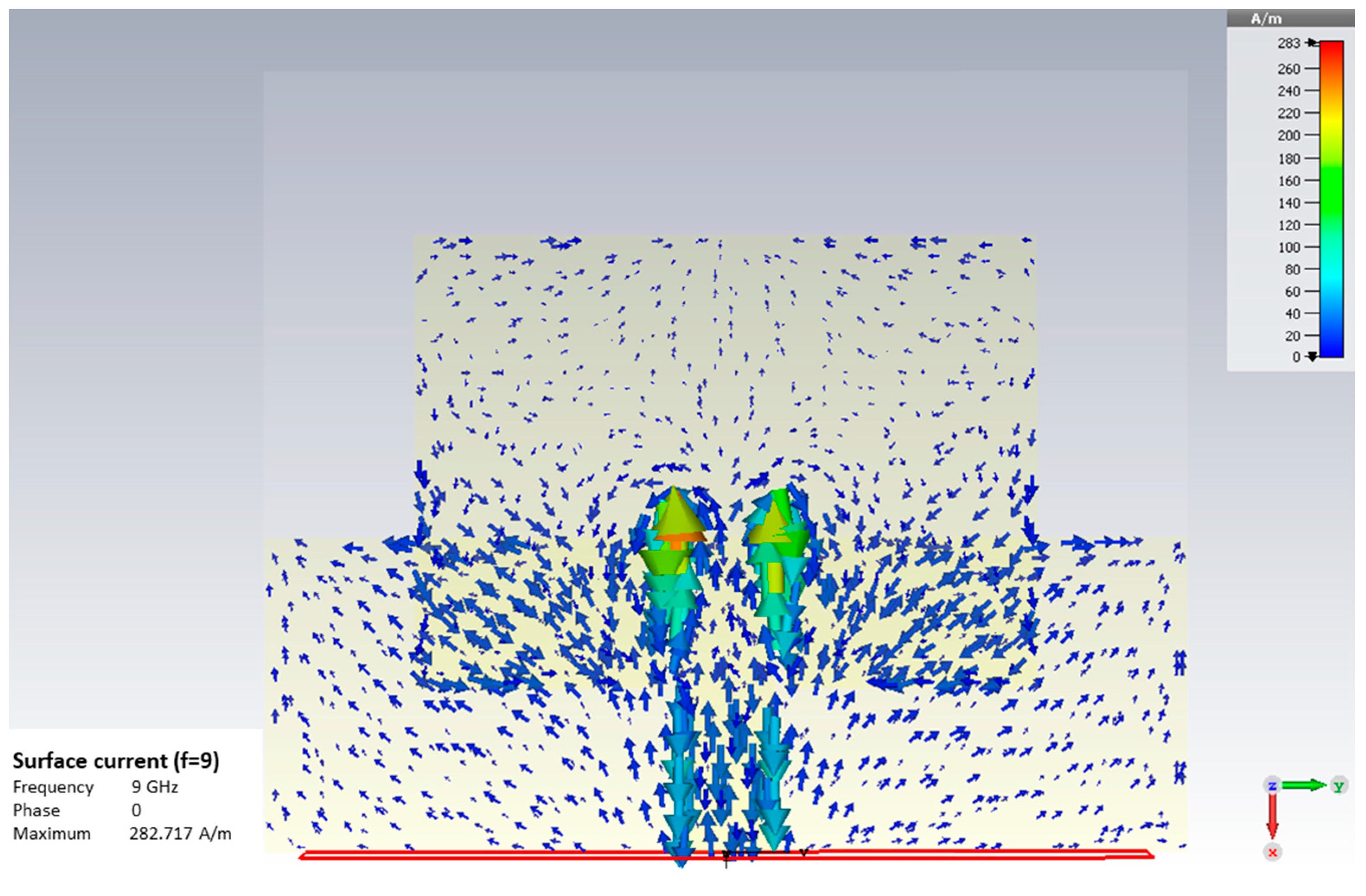
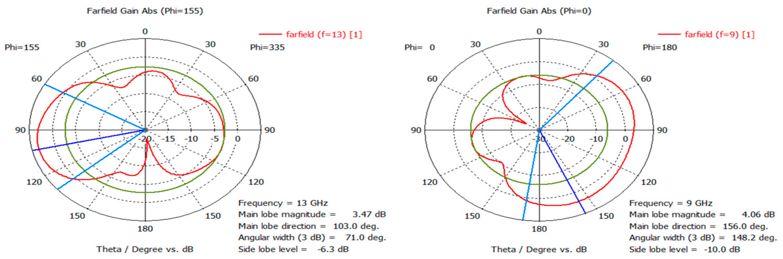
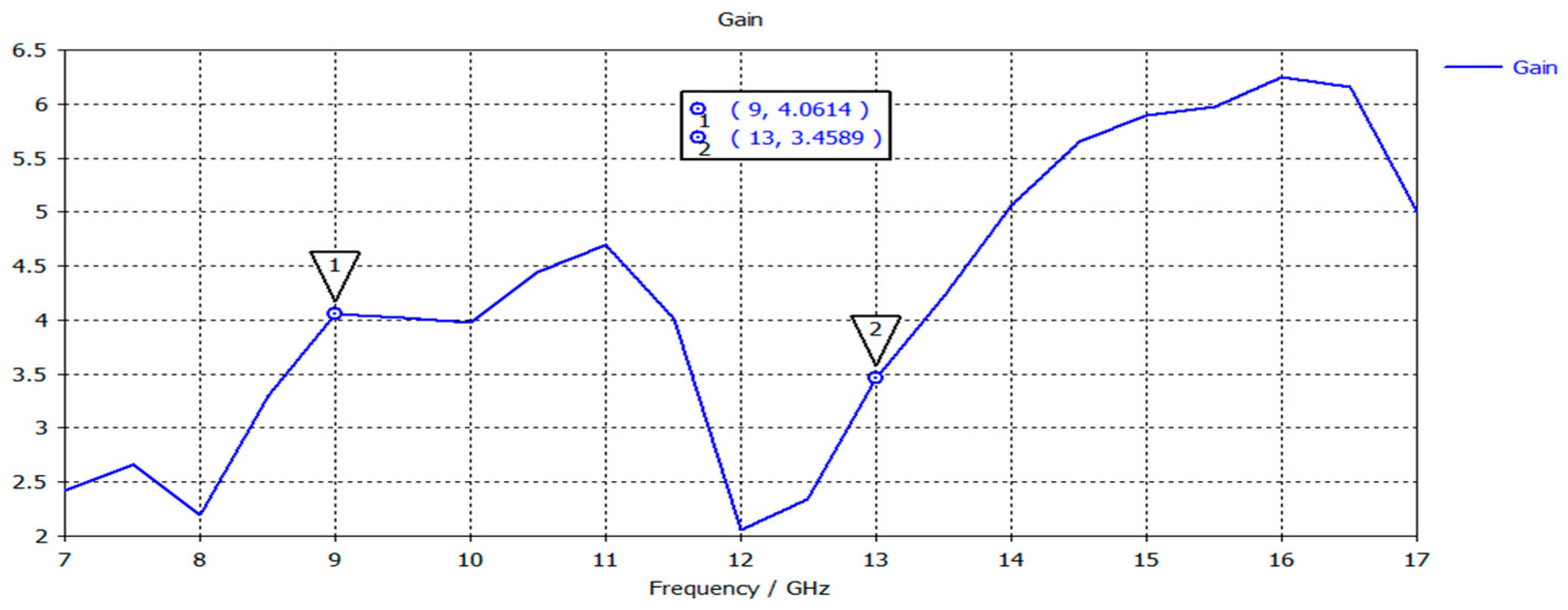
3.1. Simulated and Measured Results

The simulated and measured S11 plot is shown in Figure 3. The simulated and measured S11 plot ensures that the proposed MPA will provide satisfactory performance across the whole X-band. Moreover, the S11 graph shows that the antenna will be suitable for the entire X-band and a portion of the lower part of the Ku-band. The MPA provides two resonance frequencies of 9 GHz and 13 GHz with return loss magnitudes of S11 −35 dB and −18 dB, respectively. The MPA offers a −10 dB impedance bandwidth of 5.8 GHz, ranging from 8.35 GHz to 14.15 GHz. However, the measured return loss graph is slightly different from the simulated return loss graph. It may have occurred because the antenna is excited using a waveguide port during simulation, but practically the antenna is excited using the SMA connector. The connector loss influences the response of the antenna. In addition, the near-field scattering objects, the losses due to the feed connector, and the coaxial cable also affect the response of the antenna performance. Figure 4 shows that the VSWR is less than 1.5 at both resonance frequencies, ensuring good impedance matching characteristics.
The surface current distribution of the designed MPA indicates that the antenna has the most current in the middle of its length and the least current near its edges, as illustrated in Figure 5. To validate the simulated and measured S11, the equivalent RLC model of the proposed antenna is designed using Agilent ADS software and the resonance frequencies obtained from the RLC equivalent model of the proposed MPA using ADS Agilent software are almost equal to the simulated (using CST) and measured resonance frequencies. In addition, the S11 using ADS is −34 dB and −35 dB at both resonance frequencies.
The radiation pattern of the proposed antenna is depicted in Figure 6, which shows the main lobe direction, main lobe magnitude, side lobe level (SLL), and a 3-dB beam width. At the two distinct resonance frequencies, the 3-dB beam width is 148.2 degrees for 9 GHz and 71 degrees for 13 GHz. The SLL at a resonance frequency of 13 GHz is −6.3 dB and at a frequency of 9 GHz it is −10 dB. Gain is a measurement of the energy delivered to the main beam. The gain vs. frequency curve of the proposed antenna is presented in Figure 7. From the figure, the gain of the microstrip patch antenna varies from 2.2 dB to 6.25 dB in the entire simulated frequency range. The designed antenna gained 4.0614 dB at 9 GHz and 3.4589 dB at 13 GHz.

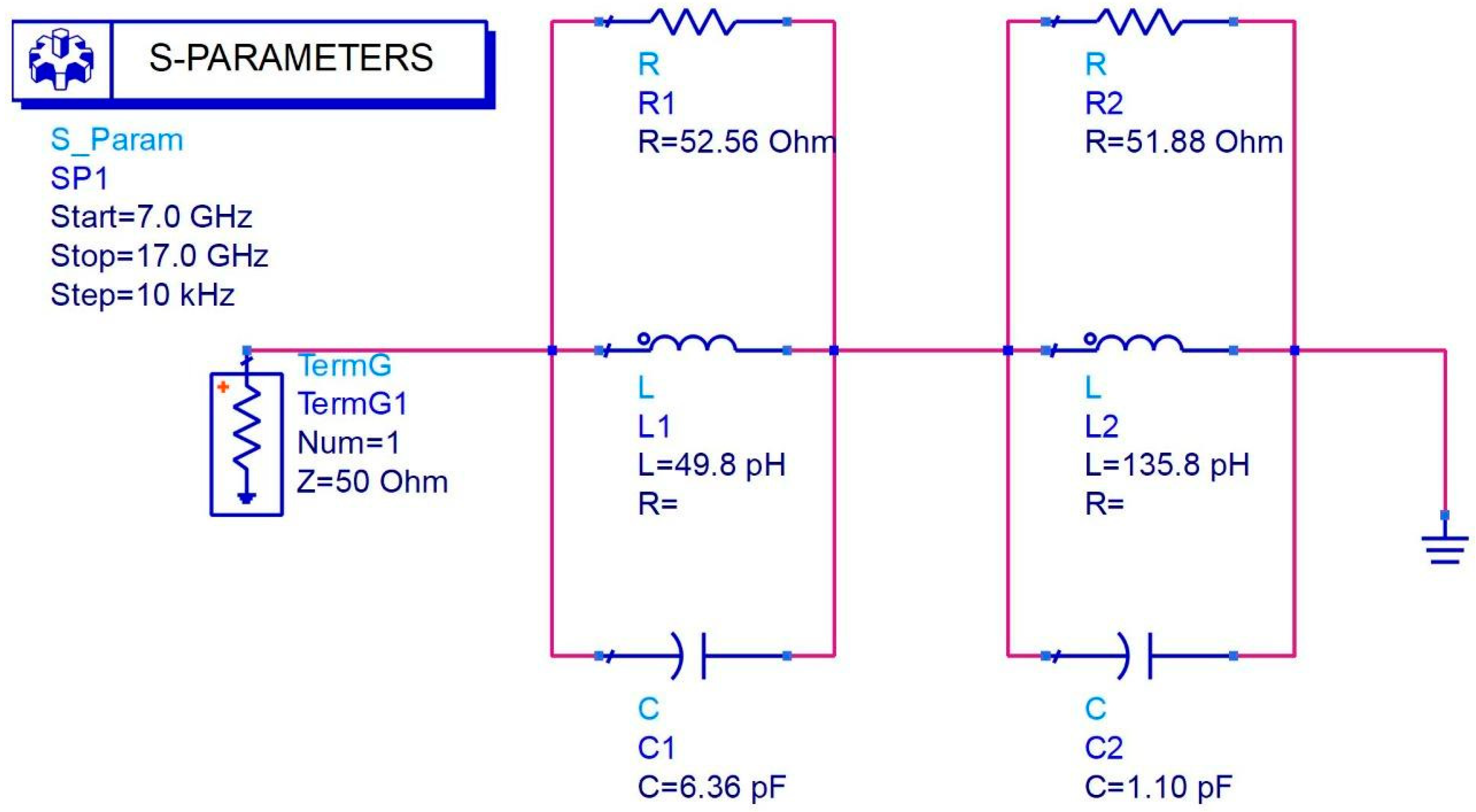
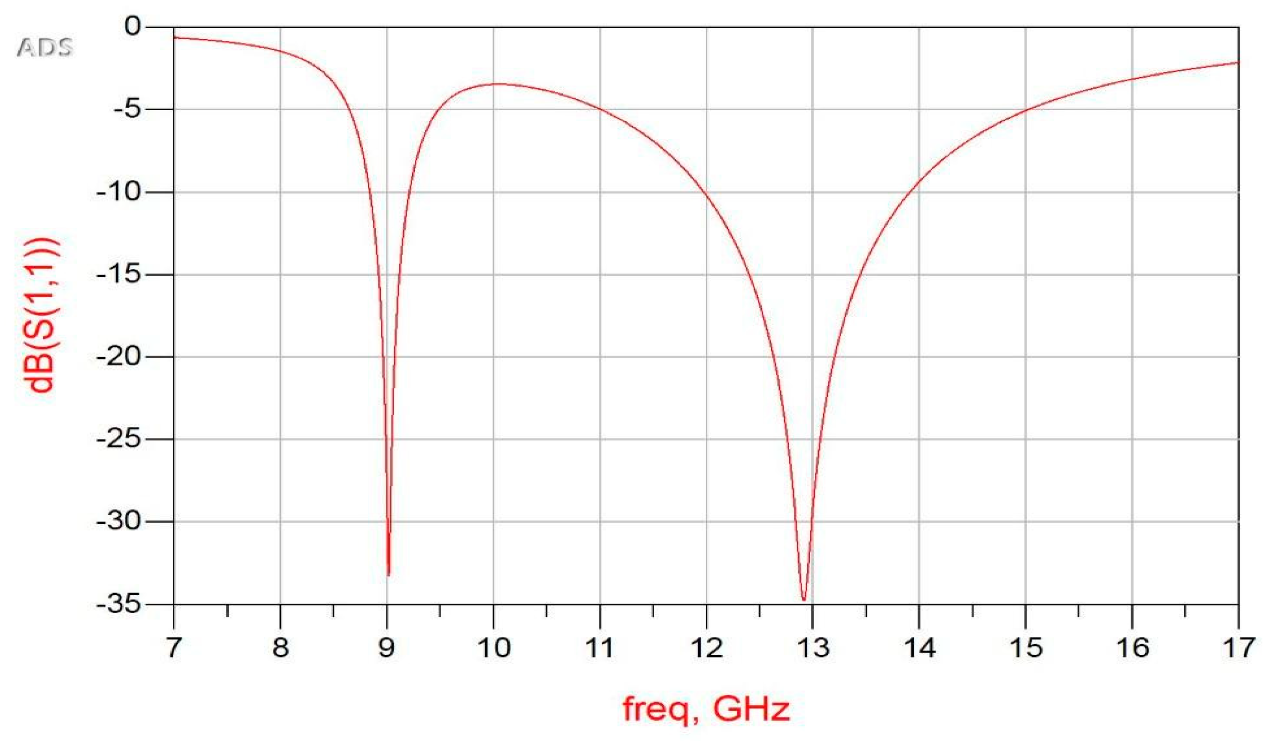
3.2. RLC Lumped Element Extraction and Equivalent Circuit of the Proposed MPA Using ADS

The equivalent RLC model of the proposed MPA using Agilent ADS software is presented in Figure 8. The values of R, L, and C have been chosen so that the equivalent impedance of the designed antenna is reasonably matched with the characteristic impedance (50 Ω) of the transmission line. An optimal impedance match between the antenna and the transmission line is required to transfer maximum power from the input port of the antenna to its antenna structure [35]. For the resonance frequencies of 9 GHz and approximately 13 GHz, resistance R 1 = 52.56   Ω , inductance L 1 = 49.8   pH , and capacitance C 1 = 6.369   pF are assigned to the parallel RLC circuit, along with resistance R 2 = 51.88   Ω , inductance L 2 = 135.8   pH , and capacitance C 2 = 1.10   pF as presented in Figure 8. As the antenna input port, the input terminal source in ADS is configured as a terminal block (Term is G) with a 50 Ω characteristic impedance and acts as an input port for the antenna. The values of R, L, and C are considered in such a manner that the equivalent circuit impedance is equal to the antenna input port impedance. The impedance matching performance is observed in ADS using the S-parameter block. In the S-parameter block, the intended frequency range is swept from 7 GHz to 17 GHz in 10 KHz increments. The plot of the return loss response (dB (S (1,1)) is chosen for plotting the resonant circuit’s output result. The resonant circuit yields a resonant frequency of 9.0 GHz with a return loss of −33 dB, and at 13 GHz with a return loss of -35 dB, as shown in Figure 9.

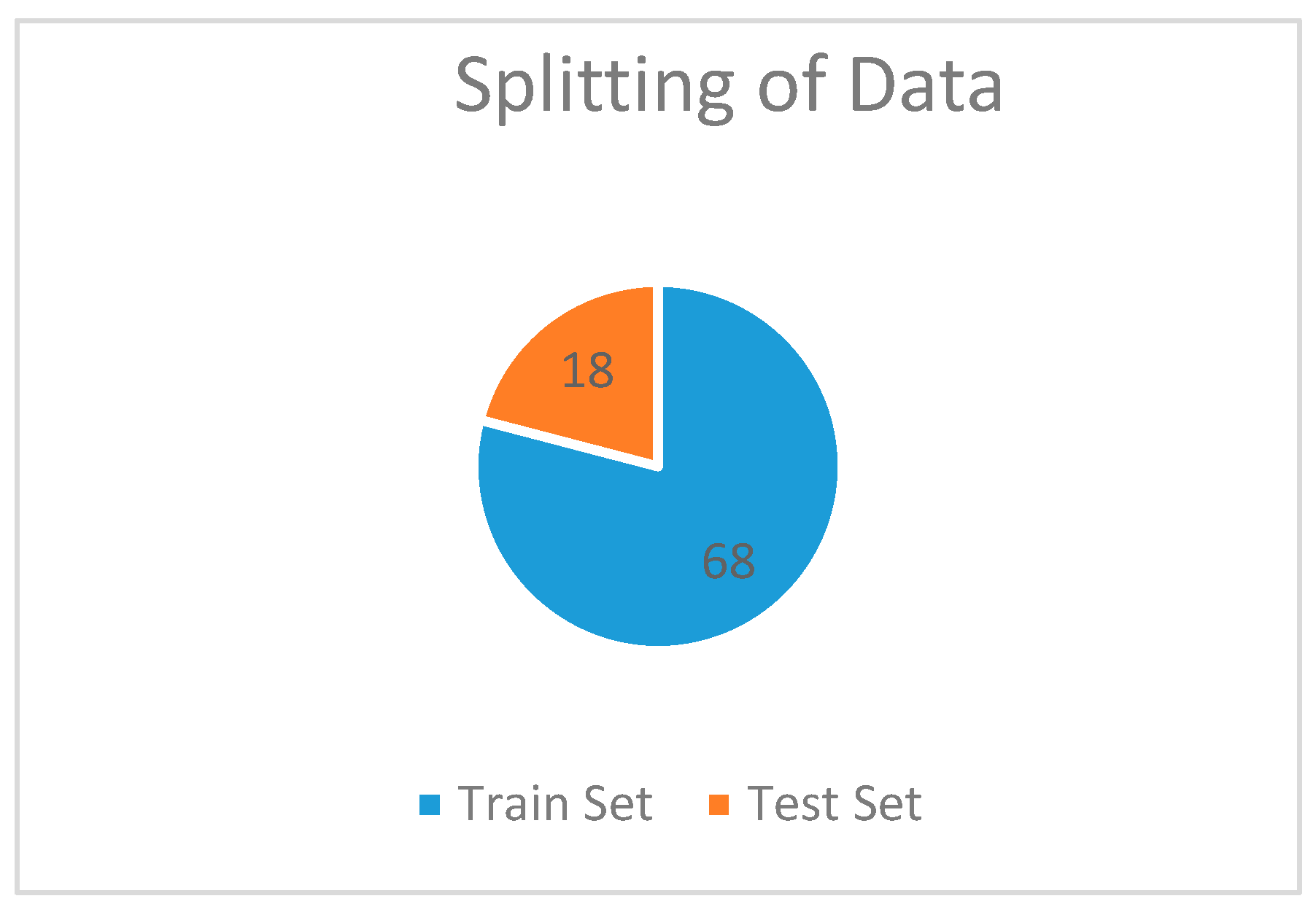
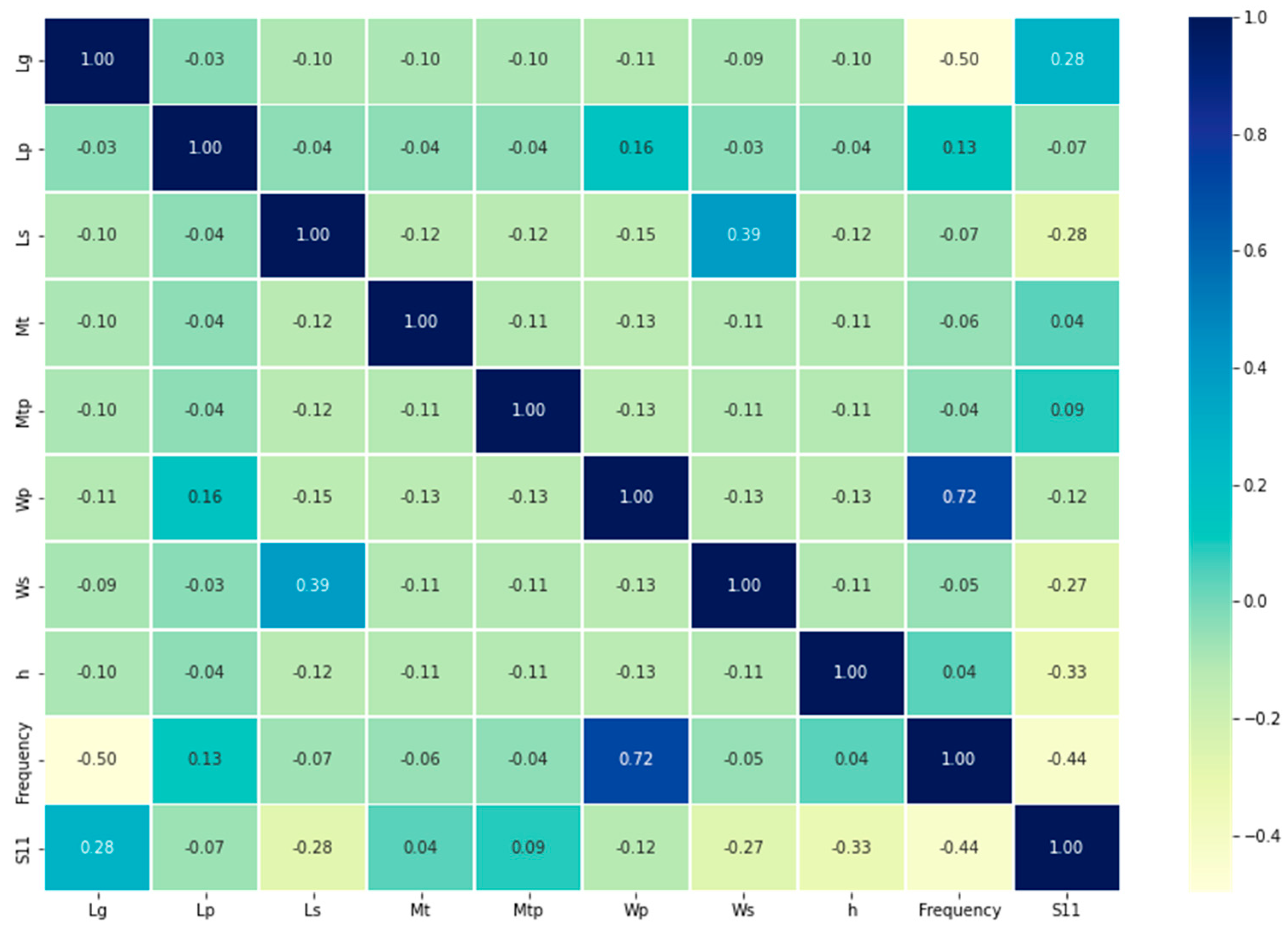
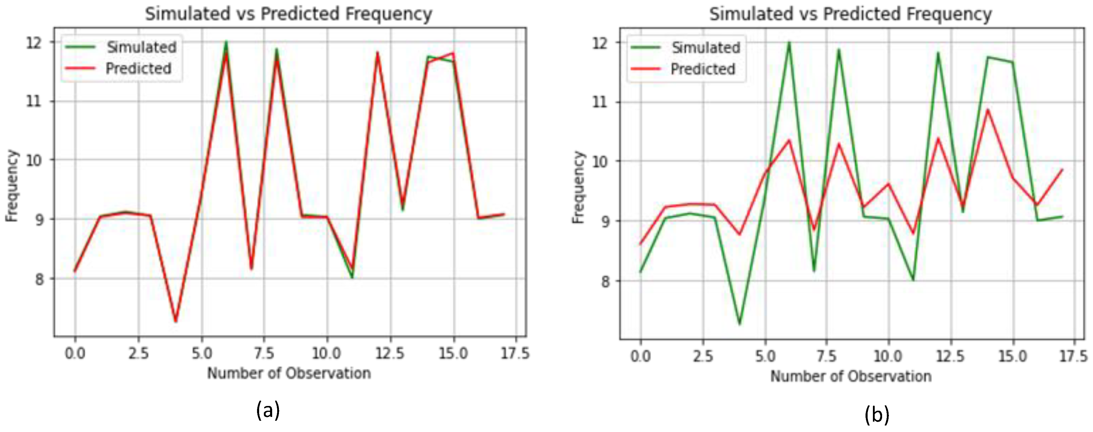
3.3. Machine Learning-Based Resonance Frequency Prediction

To achieve simplicity in the design of the antenna and predict the antenna performances, different ML and/or DL models are introduced. Using those models, the design and optimization of the antennas are much easier than with the traditional EM simulation tools. In this study, we are investigating and showing a wide variety of regression methods along with convolutional neural networks (CNN). All these algorithms are used to predict the resonance frequency of the proposed MPA. A brief description of the different models that are used for the prediction of resonance frequency is provided in the following subsection.

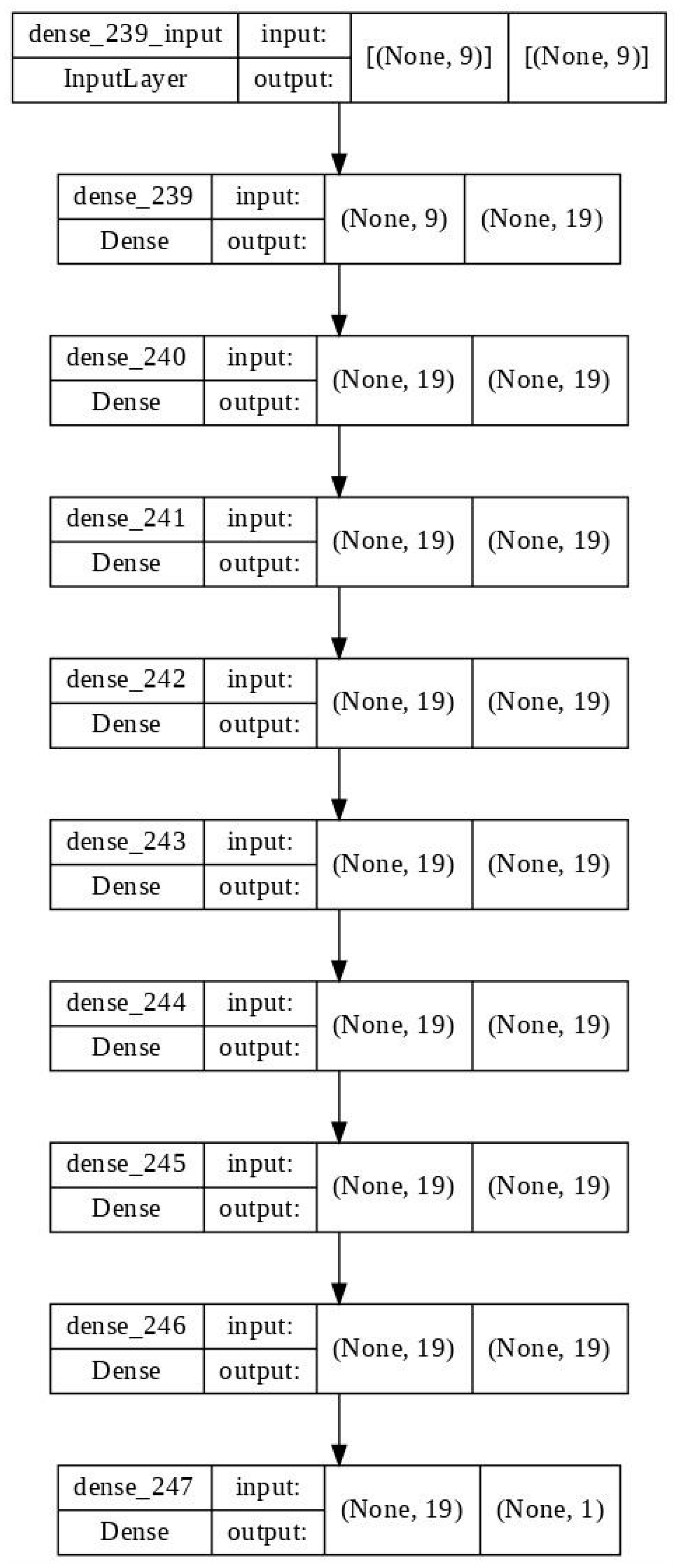
4. Brief Description of the Learning Models

Machine Learning Models:
Machine learning creates algorithms from data and then uses those algorithms to generate predictions based on other data. Multiple methods, including regression, classification, and deep learning, see heavy rotation in the machine learning toolkit (Neural Network). To solve this problem, we are investigating and showing various regression methods. It is common practice to employ regression when making predictions and forecasts.
Convolutional Neural Network (CNN):
CNN has been proposed for use on one-dimensional data in addition to its widespread application in image recognition and text analysis. In convolutional neural networks, there are three types of layers: input, hidden, and output. Both the input and output layers are activated linearly. However, since neural networks can have multiple hidden layers, their activation functions are often nonlinear. Hidden layers in convolutional neural networks (CNNs) convolve the input and send the result to the next layer [36,37]. Table 2 shows the hyperparameter settings of the CNN model. The CNN architecture is shown in Figure 10.
Linear Regression:
Linear regression is a well-known approach in the fields of statistics and machine learning. This is a mathematical technique used in forecasting or predicting results. A linear regression model aims to establish a correlation between a set of characteristics and a continuous dependent variable [38].
Random Forest Regression:
Classification and regression with random forests involve constructing a set of tree predictors, each of which is built with a random vector that is chosen independently of the input vector. Regression with tree predictor uses numerical values in place of class labels. Random forest regression constructs a tree when using variables at each node [39].
Decision Tree Regression:
Decision tree regression considers an object’s qualities and trains a model to predict future data and give useful continuous output. It is a tree structure for quantitatively forecasting the results of the dependent variable [40].
Lasso Regression:
Lasso regression is one type of linear regression that employs the shrinkage method. Researchers often turn to lasso regressions for modeling scenarios with many features [41] because of its efficiency in executing feature selection.
Ridge Regression:
A valuable method for analyzing multiple regression on data that exhibits multicollinearity is known as ridge regression. It is a regularization model where an extra variable (tune parameter) is added and optimized to address numerous variables in linear regression [42].
XGB Regression:
When it comes to fixing regression or classification issues, the most efficient method is extreme gradient boosting (XGBoost). This approach uses a gradient boosting framework to make use of decision trees. It provides features that significantly affect the model’s efficacy [43].
The data generation flow diagram is shown in Figure 11. There are six regression models, linear regression, random forest regression, decision tree regression (DTR), lasso regression, ridge regression, XGB regression, and CNN, used to predict the resonance frequency. The comparisons between the simulated and the predicted resonance frequencies of the 18 test data samples using DTR and CNN are shown in Table 3 and Table 4, respectively

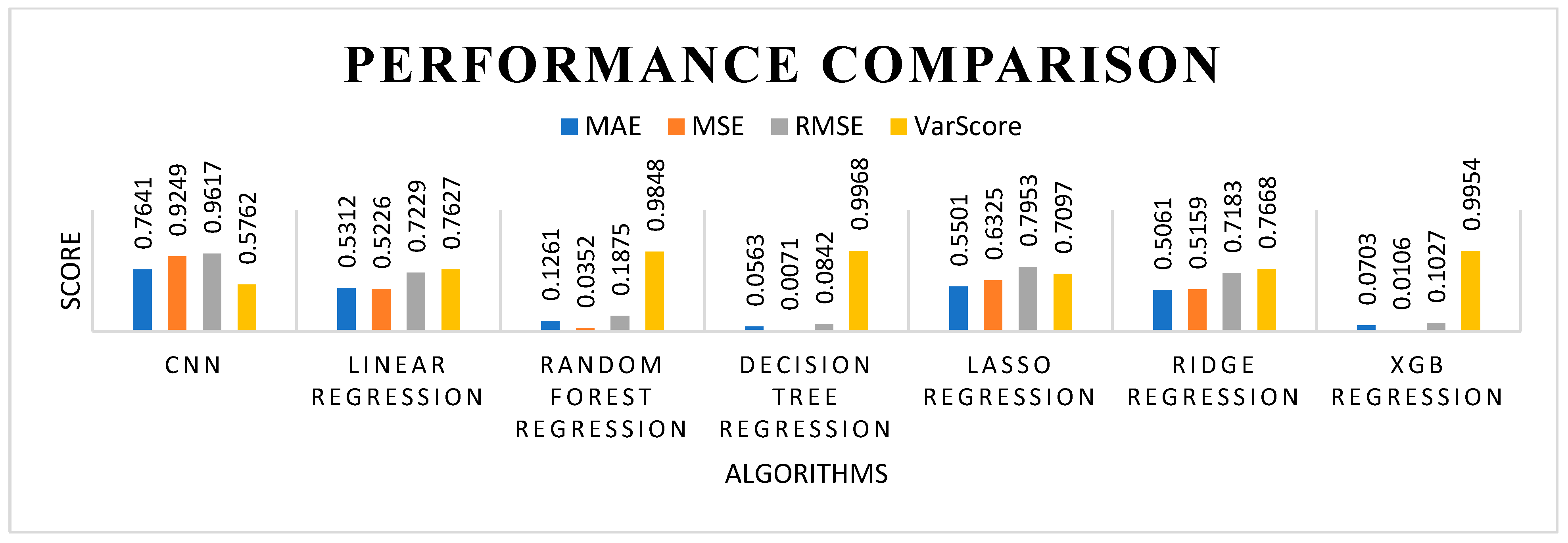
Performance Evaluation of the ML Models

Different performance metrics of the ML models are investigated to validate the prediction of the resonance frequency with respect to the simulated and the measured resonance frequency. In this research work, the mean absolute error (MAE), the mean squared error (MSE), the root mean squared error (RMSE), and the variance score are observed as performance indicators of the ML regression models. Predicting errors are computed, and prediction models are assessed using these metrics. The mean absolute error, mean squared error, and root-mean-squared error are well-known scale-dependent measurements based on absolute and squared values [44,45]. The MAE considers the average amount of error over a group of projections but ignores the direction of the mistake, giving less weight to extreme predictions [46]. In [47], the MAE is mathematically formulated as:
M A E = 1 n   i = 1 n P i O i  
where n = number of errors and P i O i = Absolute error.
The MSE is a common statistic used in estimation. The root-mean-squared error (RMSE) is used in place of MSE by taking the square root. The root-mean-squared error (RMSE) quantifies how far estimates deviate from reality. The definition of RMSE is [48]:
R M S E = 1 n   i = 1 n P i O i 2
Another performance indicator is the explained variance score that reflects the error scatter in a data collection. It can be defined as [49]:
e x p l a i n e d   v a r i a n c e y , y ^ = 1 V a r y y ^ V a r y
Figure 12 shows that a total of 86 samples were used to predict the resonance frequency of the designed MPA. Among the 86 samples, 68 samples were used to train the models and 18 samples were used to test the models’ performance. The number of training samples and the number of sampling data determines the accuracy of the prediction model. The 86 data samples were generated using CST simulation software by varying the different dimensional parameters of the proposed MPA.
Figure 13 shows a heat map plot (correlation matrix) which represents each of the ten attributes of antenna design parameters named Lp, Ls, Lg, Wp, h, Ws, Mtp, Mt, S11, and frequency on the y- and x-axis of the plot. These values represent the input dimensions of the proposed antenna structure, as shown in Table 1 and Figure 2 in the previous section. The maximum correlation occurs at the center of the plot with a value of 1.00. As the point moves away from the maximum line (1.00), the correlation decreases accordingly. In this mapping plot, the correlation value ranges from 0.03 to 0.72.
Figure 14 shows the simulated vs. predicted frequency of test data samples using DTR and CNN, respectively, for 18 test samples. In the analysis, the frequency tuning ranges from 7 GHz to 12 GHz. It is shown in Figure 14a that there is a small deviation (close to 0) between the actual and predicted frequencies for DTR. Among the 18 test samples, 3 test samples were accurately predicted, with zero percentage of error. In addition, the percentage of error in most cases is less than one. As a result, the predicted result almost perfectly matches the simulated result, as shown in Figure 14a. Somehow, there are deviations for CNN with magnitudes ranging from 0.95446% to 20.65657% as depicted in Figure 14b. It is found that the percentage of predicted errors in CNN is slightly higher than in DTR. Hence, DTR is selected for better prediction performance as compared to CNN.
The performance metrics of ML for CNN, linear regression, random forest regression, decision tree regression (DTR), lasso regression, ridge regression, and XGB regression algorithms are tabulated in Table 5. The magnitude values of MAE, MSE, RMSE, and the variant score are evaluated to determine the error performance of each algorithm. It is shown that the DTR model generates a small percentage error for MAE, MSE, RMSE, and the variant score magnitude with values of 5.63%, 0.71%, 8.42%, and 99.68%, respectively. The DTR method has performed better than the rest of the regression models and yields the highest quality results in all four scenarios. It is also shown that the XGB model is considered as a secondary selection, where it generates values of 7.03%, 1.06%, 10.27%, and 99.54%, respectively. It depicts the XGB model, performing close to DTR. Somehow, the performance of the CNN and Lasso models produced lower percentage magnitudes of 76.41%, 92.49%, 96.17%, and 57.62% and 55.01%, 63.25%, 79.53%, and 70.97%, respectively. Hence, they are not good for method selection for proposed research work. The performance comparison for all algorithms viewed in the bar chart is illustrated in Figure 15.

5. Conclusions

This article discusses the integration of simulation, measurement, development of the RLC equivalent circuit model, and applying machine learning approaches to evaluate the performance of the proposed antenna. In terms of frequency, the designed antenna supports the whole X-band as well as some portions of the Ku-band. The prototype was built and analyzed to confirm the intended performance. In addition, the RLC equivalent model of the proposed MPA designed with the ADS Agilent software yields resonance frequencies nearly identical to those generated by simulation (with CST) and measurement. Furthermore, six machine learning and one deep learning (CNN) algorithm have been developed to determine the resonant frequency of the MPA. When the predicted and simulated resonant frequencies are compared, it is observed that they are almost identical. Different performance metrics, such as MAE, MSE, RMSE, and variance scores, are calculated to validate the prediction using the learning algorithms. These metrics are obtained through the process of computing the results of the prediction. The predicted results show that the error performances of the decision tree regression model are comparatively better than other models. The MAE, MSE, RMSE, and variance scores (in percentage) of the DTR model are 5.63, 0.71, 8.42, and 99.68, respectively. The XGB model (MAE = 7.03%, MSE = 1.06%, RMSE = 10.27%, and var score = 99.54%) performs better than the other learning models that were introduced in this study, except DTR. The performance of the deep learning model (CNN) is slightly lower than the presented regression models, which may have occurred due to the inadequate number of data samples for the CNN model. Despite the fact that the proposed MPA has two resonant frequencies, we have only predicted one (9 GHz) using ML models. In addition, the designed MPA has a lower gain of 4.06 dB at 9 GHz and 3.46 dB at 13 GHz. The measured resonance frequency range (7.90 GHz to 14.6 GHz) does not quite correspond to the predicted resonance frequency range (8.35 GHz to 14.25 GHz). In the future, we will generate an adequate number of data samples to achieve better results using DL models, such as CNN, and predict the multiple frequencies for a multiband antenna. Furthermore, we will develop the ML models to predict the return loss, gain, length, and width of the proposed antenna. Moreover, we will ensure better impedance matching between the proposed MPA and the SMA connector so that the simulated and measured frequencies are completely matched. Finally, it can be concluded that the simulated, measured, and predicted results ensure the reliability of the proposed antenna in the whole X-band and part of Ku-band applications.

Author Contributions

M.A.H. and N.S. presented the idea, performed the experiments, prepared the manuscript and visualization, N.S.S.S. prepared funding acquisition. M.A.R. and L.C.P. prepared the data curation and formal analysis, M.N.H. and M.I. described the investigation and methodology. M.A.Z. contributed to the supervision of the research work. G.E.M.A. and A.H.S. contributions include software development, resources, and validation. M.H. and R.P. contributed to writing and reviewing. All authors have read and agreed to the published version of the manuscript.

Funding

Regarding software simulation, this research was sponsored by INTI International University, Malaysia, and they sponsored this research work from the beginning till publication.

Institutional Review Board Statement

Not applicable.

Informed Consent Statement

Not applicable.

Data Availability Statement

Not applicable.

Acknowledgments

The author wishes to extend his sincere thanks to the support of the Centre of Graduate Studies, Universitiy Teknologi, PETRONAS, Malaysia, and the Faculty of Data Science and Information Technology at INTI International University, Malaysia, for providing the state-of-the-art research facilities to carry on this work. In addition, the author is also thankful for the support provided by the collaborators from Condition Monitoring System, National Center of Robotics and Automation, Mehran University of Engineering and Technology, Jamshoro, Sindh, Pakistan. The entire project was sponsored by the Faculty of Data Science and Information Technology, INTI International University, Malaysia, for the necessary results.

Conflicts of Interest

The authors declare no conflict of interest.

References

  1. Paul, L.C.; Ali, H.; Sarker, N.; Mahmud, Z.; Azim, R.; Islam, M.T. A Wideband Rectangular Microstrip Patch Antenna with Partial Ground Plane for 5G Applications. In Proceedings of the 2021 Joint 10th International Conference on Informatics, Electronics & Vision (ICIEV) and 2021 5th International Conference on Imaging, Vision & Pattern Recognition (icIVPR), Kitakyushu, Japan, 16–20 August 2021. [Google Scholar]
  2. Kannadhasan, S.; Nagarajan, R. Performance Improvement of S-shaped for Wireless Communication. In Electronic Systems and Intelligent Computing; Springer: Singapore, 2022; pp. 15–22. [Google Scholar]
  3. Chowdhury, S.G.; Arefin, M.S.; Faisal, M.M.A. Design Simulation and Analysis of a Dual Band Microstrip Patch Antenna for GPS and WLAN Applications. 2021. Available online: http://dspace.iiuc.ac.bd:8080/xmlui/handle/123456789/3105 (accessed on 10 August 2022).
  4. Le, D.; Ahmed, S.; Ukkonen, L.; Björninen, T. A Small All-Corners-Truncated Circularly Polarized Microstrip Patch Antenna on Textile Substrate for Wearable Passive UHF RFID Tags. IEEE J. Radio Freq. Identif. 2021, 5, 106–112. [Google Scholar] [CrossRef]
  5. Paul, L.C.; Sarkar, A.K.; Haque, A.; Miah, P.; Ghosh, P.M.; Islam, R. Investigation of the dependency of an inset feed rectangular patch antenna parameters with the variation of notch width for WiMax applications. In Proceedings of the 2018 Second International Conference on Electronics, Communication and Aerospace Technology (ICECA), Coimbatore, India, 29–31 March 2018. [Google Scholar]
  6. Huang, G.S.; Li, S.J.; Li, Z.Y.; Liu, X.B.; Di, L.R.J.; Cao, X.Y. Coding-Feeding Metasurface for Diffusion and Dual-Band Emission. Adv. Theory Simul. 2022, 5, 2200006. [Google Scholar] [CrossRef]
  7. Shi, C.; Zou, J.; Gao, J.; Liu, C. Gain Enhancement of a Dual-Band Antenna with the FSS. Electronics 2022, 11, 2882. [Google Scholar] [CrossRef]
  8. Muntoni, G.; Montisci, G.; Casula, G.A.; Chietera, F.P.; Michel, A.; Colella, R.; Catarinucci, L.; Mazzarella, G. A curved 3-D printed microstrip patch antenna layout for bandwidth enhancement and size reduction. IEEE Antennas Wirel. Propag. Lett. 2020, 19, 1118–1122. [Google Scholar] [CrossRef]
  9. Bansal, A.; Gupta, R. A review on microstrip patch antenna and feeding techniques. Int. J. Inf. Technol. 2020, 12, 149–154. [Google Scholar] [CrossRef]
  10. Fouany, J.; Thevenot, M.; Arnaud, E.; Torres, F.; Menudier, C.; Monediere, T.; Elis, K. New concept of telemetry X-band circularly polarized antenna payload for cubesat. IEEE Antennas Wirel. Propag. Lett. 2017, 16, 2987–2991. [Google Scholar] [CrossRef]
  11. Khac, K.N.; Phong, N.D.; Manh, L.H.; Le Trong, T.A.; Le Huu, H.; Hien, B.T.T.; Chien, D.N. A design of circularly polarized array antenna for X-band cubesat satellite communication. In Proceedings of the 2018 International Conference on Advanced Technologies for Communications (ATC), Ho Chi Minh City, Vietnam, 18–20 October 2018; pp. 53–56. [Google Scholar]
  12. Ganaraj, G.; Kumar, C.; Kumar, V.S. High gain circularly polarized resonance cavity antenna at X-band. In Proceedings of the 2017 IEEE International Conference on Antenna Innovations & Modern Technologies for Ground, Aircraft and Satellite Applications (iAIM), Bangalore, India, 24–26 November 2017; pp. 1–5. [Google Scholar]
  13. Trentini, G.V. Partially reflecting sheet arrays. IRE Trans. Antennas Propag. 1956, AP-4, 666–671. [Google Scholar] [CrossRef]
  14. Asaadi, M.; Sebak, A. Gain and bandwidth enhancement of 2 × 2 square dense dielectric patch antenna arrays using a Holey superstrate. IEEE Antennas Wirel. Propag. Lett. 2017, 16, 1808–1811. [Google Scholar]
  15. Razi, Z.M.; Rezaei, P. Fabry–Perot cavity antenna based on capacitive loaded strips superstrate for X-band satellite communication. Adv. Radar Syst. J. 2013, 2, 26–30. [Google Scholar]
  16. Gupta, R.; Mukherjee, J. Effect of superstrate material on a high-gain antenna using array of parasitic patches. Microw. Opt. Technol. Lett. 2010, 52, 82–88. [Google Scholar] [CrossRef]
  17. Orr, R.; Goussetis, G.; Fusco, V. Design method for circularly polarized Fabry–Perot cavity antennas. IEEE Trans. Antennas Propag. 2014, 62, 19–26. [Google Scholar] [CrossRef] [Green Version]
  18. Rahman, M.N.; Islam, M.T.; Misran, N.; Samsuzzaman, M. A tuning fork-shaped microstrip patch antenna for X-band satellite and radar applications. In Proceedings of the 2017 6th International Conference on Electrical Engineering and Informatics (ICEEI), Langkawi, Malaysia, 25–27 November 2017; pp. 1–2. [Google Scholar]
  19. Ogurtsov, S.; Koziel, S. A conformal circularly polarized series-fed microstrip antenna array design. IEEE Trans. Antennas Propag. 2019, 68, 873–881. [Google Scholar] [CrossRef]
  20. Alkaraki, S.; Gao, Y.; Stremsdoerfer, S.; Gayets, E.; Parini, C.G. 3D printed corrugated plate antennas with high aperture efficiency and high gain at X-band and Ka-band. IEEE Access 2020, 8, 30643–30654. [Google Scholar] [CrossRef]
  21. Ccoillo-Ramos, N.R.; Aboserwal, N.; Qamar, Z.; Salazar-Cerreno, J.L. Improved Analytical Model for a Proximity Coupled Microstrip Patch Antenna (PC-MSPA). IEEE Trans. Antennas Propag. 2021, 69, 6244–6252. [Google Scholar] [CrossRef]
  22. Kim, J.H.; Choi, S.W. A Deep Learning-Based Approach for Radiation Pattern Synthesis of an Array Antenna. IEEE Access 2020, 8, 226059–226063. [Google Scholar] [CrossRef]
  23. El Misilmani, H.M.; Naous, T.; Al Khatib, S.K. A review on the design and optimization of antennas using machine learning algorithms and techniques. Int. J. RF Microw. Comput.-Aided Eng. 2020, 30, e22356. [Google Scholar] [CrossRef]
  24. Bang, J.; Kim, J.H. Predicting Power Density of Array Antenna in mmWave Applications with Deep Learning. IEEE Access 2021, 9, 111030–111038. [Google Scholar] [CrossRef]
  25. Zheng, B.; Zhang, H. Deep Learning Based Multi-layer Metallic Metasurface Design. In Proceedings of the IEEE International Symposium on Antennas and Propagation, Montreal, QC, Canada, 5–10 July 2020; pp. 2049–2050. [Google Scholar]
  26. Misilmani, H.M.E.; Naous, T. Machine Learning in Antenna Design: An Overview on Machine Learning Concept and Algorithms. In Proceedings of the 2019 International Conference on High Performance Computing & Simulation (HPCS), Dublin, Ireland, 15–19 July 2019; pp. 600–607. [Google Scholar]
  27. Erricolo, D.; Chen, P.-Y.; Rozhkova, A.; Torabi, E.; Bagci, H.; Shamim, A.; Zhang, X. Machine Learning in Electromagnetics: A Review and Some Perspectives for Future Research. In Proceedings of the 2019 International Conference on Electromagnetics in Advanced Applications (ICEAA), Granada, Spain, 9–13 September 2019; pp. 1377–1380. [Google Scholar]
  28. Yao, H.M.; Li, M.; Jiang, L. Applying Deep Learning Approach to the Far-Field Subwavelength Imaging Based on Near-Field Resonant Metalens at Microwave Frequencies. IEEE Access 2019, 7, 63801–63808. [Google Scholar] [CrossRef]
  29. Wu, Q.; Cao, Y.; Wang, H.; Hong, W. Machine-learning-assisted optimization and its application to antenna designs: Opportunities and challenges. China Commun. 2020, 17, 152–164. [Google Scholar] [CrossRef]
  30. Kushwah, V.S.; Tomar, G.S. Design and analysis of microstrip patch antennas using artificial neural network. In Trends in Research on Microstrip Antennas; IntechOpen: London, UK, 2017; p. 55. [Google Scholar]
  31. Soni, M.; Sharma, K.; Pandey, G.P.; Gupta, S.K. Resonant Frequency Prediction of Patch Antenna in the Presence of Inserted Airgap Using Machine Learning. In Advances in Smart Communication and Imaging Systems; Springer: Singapore, 2021; pp. 353–361. [Google Scholar]
  32. Aoad, A. Design and manufacture of a multiband rectangular spiral-shaped microstrip antenna using EM-driven and machine learning. Elektron. Ir Elektrotechnika 2021, 27, 29–40. [Google Scholar] [CrossRef]
  33. Balanis, C.A. Antenna Theory: Analysis and Design; John Wiley & Sons: Hoboken, NJ, USA, 2015. [Google Scholar]
  34. Barthia, P.; Rao, K.V.S.; Tomar, R.S. Millimeter Wave Microstrip and Printed Circuit Antenna; Artech House: Boston, MA, USA, 1991. [Google Scholar]
  35. Pozar, D.M. Microwave Engineering; John Wiley & Sons: Hoboken, NJ, USA, 2011. [Google Scholar]
  36. Jernelv, L.; Hjelme, D.R.; Matsuura, Y.; Aksnes, A. Convolutional neural networks for classification and regression analysis of one-dimensional spectral data. arXiv 2020, arXiv:2005.07530. [Google Scholar]
  37. Kıymık, E.; Erçelebi, E. Metamaterial Design with Nested-CNN and Prediction Improvement with Imputation. Appl. Sci. 2022, 12, 3436. [Google Scholar] [CrossRef]
  38. Manasa, J.; Gupta, R.; Narahari, N.S. Machine learning based predicting house prices using regression techniques. In Proceedings of the 2020 2nd International Conference on Innovative Mechanisms for Industry Applications (ICIMIA), Bangalore, India, 5–7 March 2020. [Google Scholar]
  39. Singh, B.; Sihag, P.; Singh, K. Modelling of impact of water quality on infiltration rate of soil by random forest regression. Model. Earth Syst. Environ. 2017, 3, 999–1004. [Google Scholar] [CrossRef]
  40. Rathore, S.S.; Kumar, S. A decision tree regression-based approach for the number of software faults prediction. ACM SIGSOFT Softw. Eng. Notes 2016, 41, 1–6. [Google Scholar] [CrossRef]
  41. Madhuri, C.H.R.; Anuradha, G.; Pujitha, M.V. House price prediction using regression techniques: A comparative study. In Proceedings of the 2019 International Conference on Smart Structures and Systems (ICSSS), Chennai, India, 14–15 March 2019. [Google Scholar]
  42. Israni, D.; Masalia, K.; Khasgiwal, T.; Tolani, M.; Edinburgh, M. Crop-yield prediction and crop recommendation system. SSRN Electron. J. 2022. [Google Scholar] [CrossRef]
  43. Torres-Barrán, A.; Alonso, Á.; Dorronsoro, J.R. Regression tree ensembles for wind energy and solar radiation prediction. Neurocomputing 2019, 326–327, 151–160. [Google Scholar] [CrossRef]
  44. Kumar, R.; Kumar, P.; Kumar, Y. Time series data prediction using IOT and machine learning technique. Procedia Comput. Sci. 2020, 167, 373–381. [Google Scholar] [CrossRef]
  45. Choo, J.; Pho TH, A.; Kim, Y.H. Machine Learning Technique to Improve an Impedance Matching Characteristic of a Bent Monopole Antenna. Appl. Sci. 2021, 11, 10829. [Google Scholar] [CrossRef]
  46. Harimurti, R.; Yamasari, Y.; Ekohariadi; Munoto; Asto, B.I.G.P. Predicting student’s psychomotor domain on the vocational senior high school using linear regression. In Proceedings of the 2018 International Conference on Information and Communications Technology (ICOIACT), Yogyakarta, Indonesia, 6–7 March 2018. [Google Scholar]
  47. Chai, T.; Draxler, R.R. Root means square error (RMSE) or mean absolute error (MAE)? Arguments against avoiding RMSE in the literature. Geosci. Model Dev. 2014, 7, 1247–1250. [Google Scholar] [CrossRef] [Green Version]
  48. Willmott, C.J.; Matsuura, K. Advantages of the mean absolute error (MAE) over the root mean square error (RMSE) in assessing average model performance. Clim. Res. 2005, 30, 79–82. [Google Scholar] [CrossRef]
  49. Weiming, J.M. Mastering Python for Finance—Second Edition. O’Reilly Online Learning. Available online: https://www.oreilly.com/library/view/mastering-python-for/9781789346466/d1ac368a-6890-45eb-b39c-2fa97d23d640.xhtml (accessed on 21 August 2022).
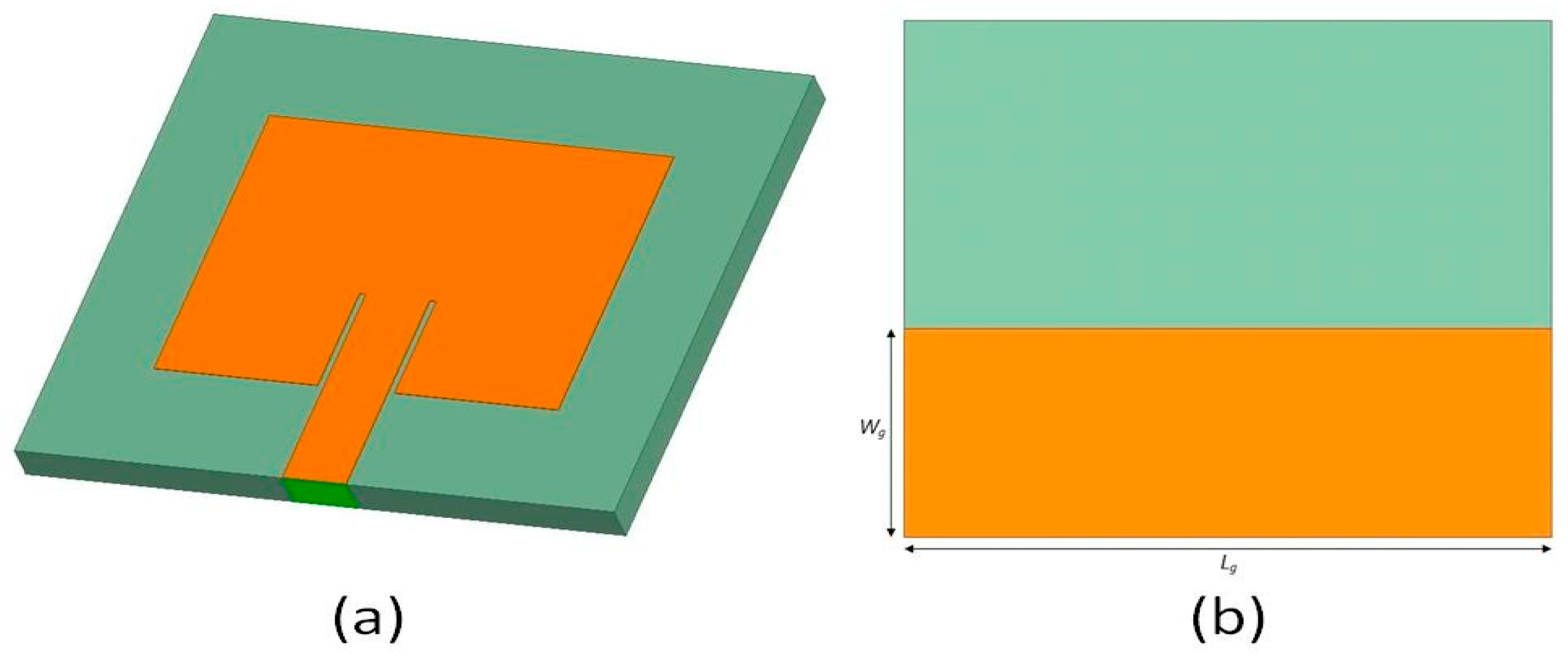
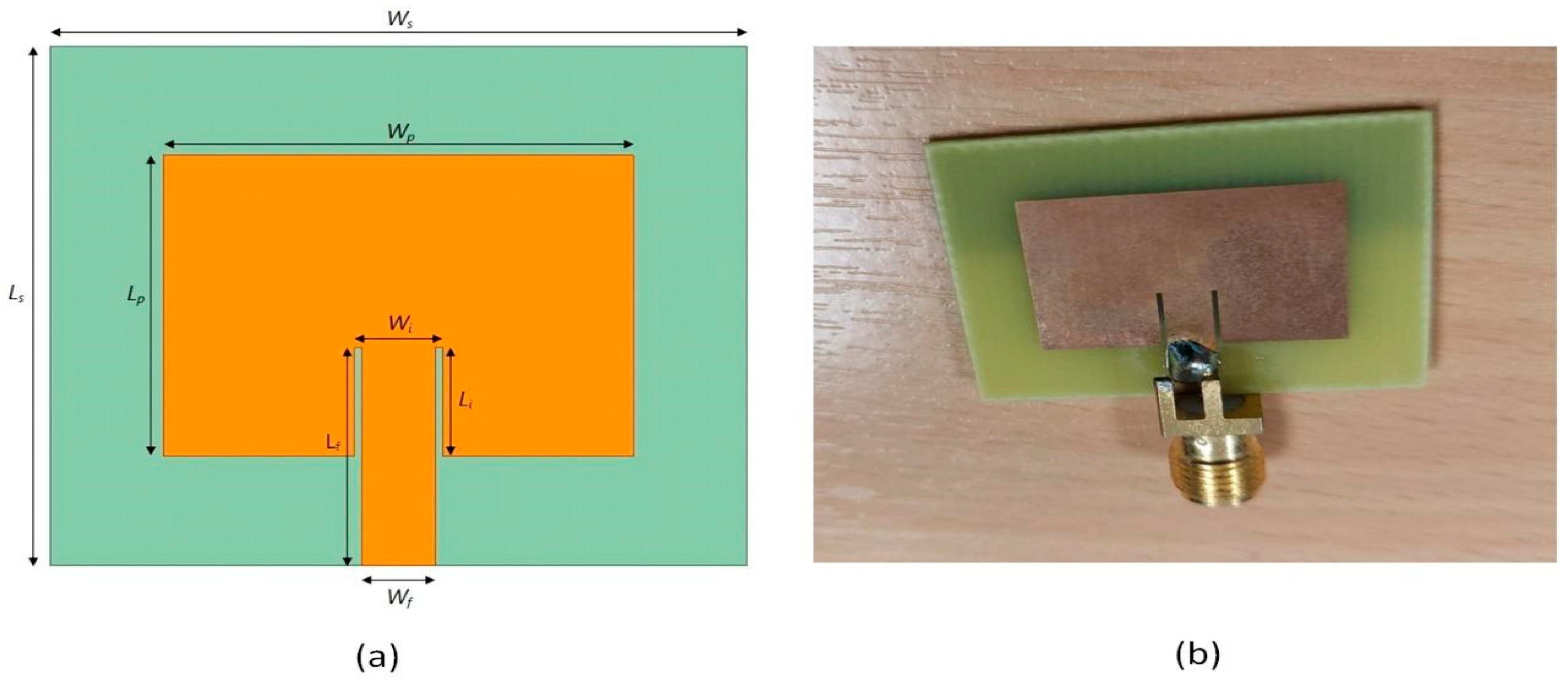
Figure 1. (a) Three-dimensional view and (b) partial ground plane of the proposed X-band MPA.
Applsci 12 10505 g001
Figure 2. (a) Front view of the proposed MPA. (b) Fabricated Prototype.
Applsci 12 10505 g002
Figure 3. Return loss (S11) vs. frequency plot of the proposed MPA.
Applsci 12 10505 g003
Figure 4. Simulated VSWR of the proposed MPA.
Applsci 12 10505 g004
Figure 5. Surface current distribution.
Applsci 12 10505 g005
Figure 6. Radiation pattern of the proposed MPA.
Applsci 12 10505 g006
Figure 7. Gain vs. frequency plot of the proposed MPA.
Applsci 12 10505 g007
Figure 8. Circuit diagram of a parallel RLC circuit for resonant frequency (refer to CST simulation) using ADS Agilent simulation.
Applsci 12 10505 g008
Figure 9. Simulated result using ADS Agilent equivalent circuit.
Applsci 12 10505 g009
Figure 10. CNN architecture.
Applsci 12 10505 g010
Figure 11. (a) Flowchart for ML/DL-based antenna results prediction; (b) analysis of MPA using ML/DL models.
Applsci 12 10505 g011
Figure 12. Pie chart for splitting the data set.
Applsci 12 10505 g012
Figure 13. Correction matrix.
Applsci 12 10505 g013
Figure 14. Simulated vs. predicted frequency using (a) DTR and (b) CNN.
Applsci 12 10505 g014
Figure 15. Comparative bar chart for seven algorithms.
Applsci 12 10505 g015
Table 1. Antenna design parameters.
ParametersFull Form of
Parameters
Dimensions (mm)ParametersFull Form of ParametersDimensions (mm)
L S Length of Substrate23.8 L f Length of Feed Line10
L G Length of Ground28.2 W f Width of Feed Line3
W G Width of Ground9.6 L i Length of Inset5
L P Length of Patch13.8 W i Width of Inset3.6
W P Width of Patch19 M t P Thickness of patch0.035
h Thickness of substrate1.6 M t Thickness of Ground0.035
W S Width of Substrate28.2---
Table 2. Hyperparameter setting for used CNN.
HyperparameterConfiguration
Dense layer’s activation functionReLU
Batch size16
Epoch100
Optimization functionAdam
LossMSE
Table 3. Simulated and predicted resonant frequency comparison of the test set using DTR.
No.Simulated Frequency (GHz)Predicted Frequency (GHz)Error
Percentage (%)
No.Simulated Frequency (GHz)Predicted Frequency (GHz)Error
Percentage (%)
18.14148.11130.3697109.0649.02850.3917
29.03969.02850.1228119.02969.02960
39.11769.09530.24461288.15261.9075
49.05079.050701311.8111.7940.1355
57.26237.26230149.14139.22960.9659
69.3519.38410.3541511.73411.6340.8522
711.98811.7941.61831611.64911.7941.2447
88.14878.15260.04791799.01730.1922
911.86511.7121.2895189.06399.07530.1258
Table 4. Simulated and predicted resonant frequency comparison of the test set using CNN.
No.Simulated Frequency (GHz)Predicted Frequency (GHz)Error
Percentage (%)
No.Simulated Frequency (GHz)Predicted Frequency (GHz)Error
Percentage (%)
18.14148.60865.73869109.0649.2221.74353
29.03969.2252.05042119.02969.61166.44494
39.11769.27571.734361288.77899.7363
49.05079.2652.367261311.8110.378712.11948
57.26238.762420.65657149.14139.22860.95446
69.3519.77524.535941511.73410.86047.44519
711.98810.345713.699461611.6499.712816.62076
88.14878.83758.452331799.26112.90101
911.86510.284413.32168189.06399.84938.6656
Table 5. The resonant frequency prediction performance of ML algorithms.
AlgorithmsMAEMSERMSEVar Score
CNN0.76410.92490.96170.5762
Linear Regression0.53120.52260.72290.7627
Random Forest Regression0.12610.03520.18750.9848
Decision Tree Regression0.05630.00710.08420.9968
Lasso Regression0.55010.63250.79530.7097
Ridge Regression0.50610.51590.71830.7668
XGB Regression0.07030.01060.10270.9954
Publisher’s Note: MDPI stays neutral with regard to jurisdictional claims in published maps and institutional affiliations.

