
A Novel Approach to Classify Telescopic Sensors Data Using Bidirectional-Gated Recurrent Neural Networks

 ,
,  , , and
Abstract
1. Introduction
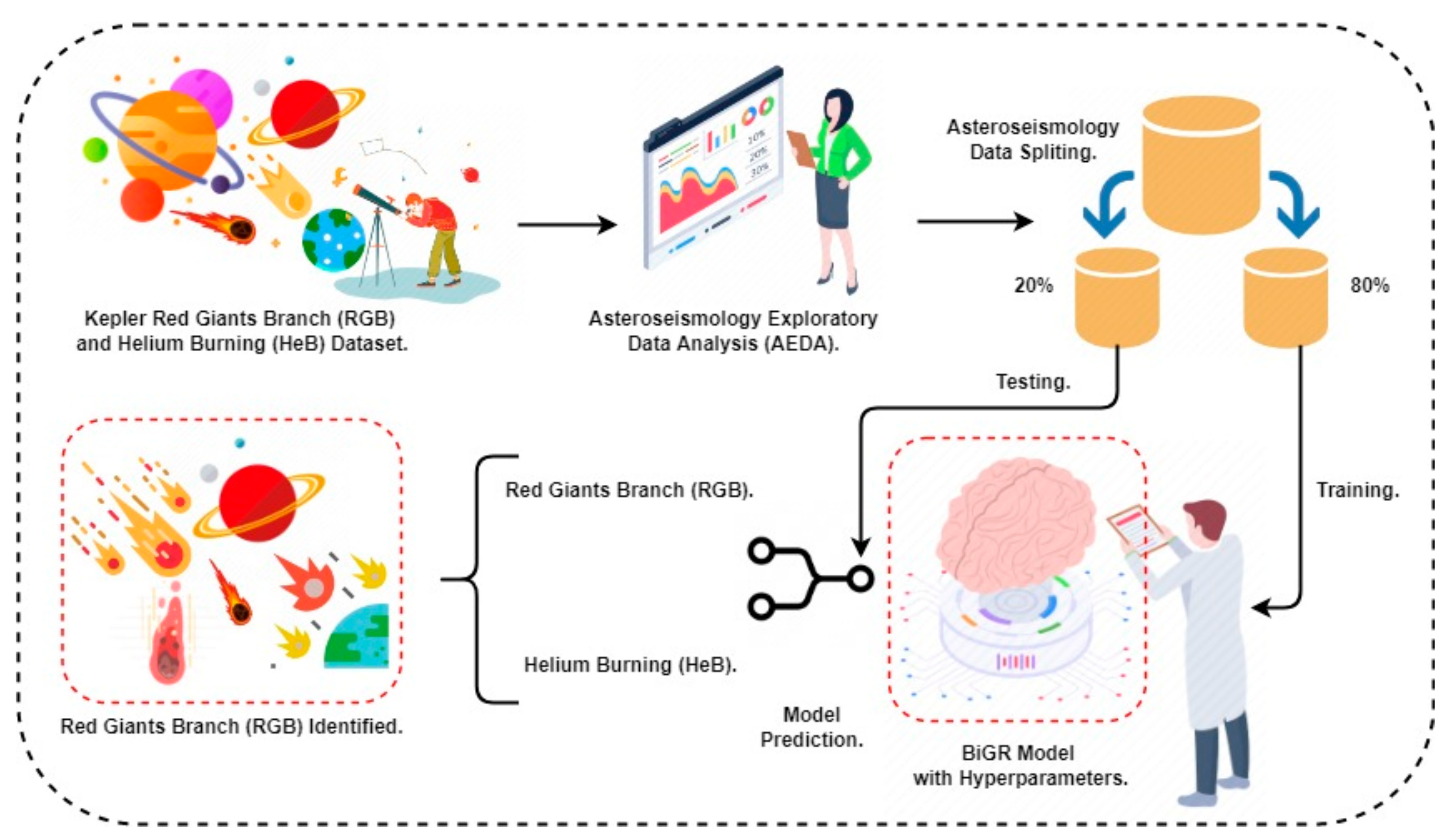
- A novel bidirectional-gated recurrent unit and recurrent neural network (BiGR)-based deep learning model is proposed to classify the RGB (red-giant branch) and HeB (helium burning);
- The Asteroseismology Exploratory Data Analysis (AEDA) is conducted to find the dataset feature patterns disorders and obtain a fruitful data visualization analysis for a better understanding of asteroseismology norms;
- A comparative analysis of the past approaches in the context of asteroseismology classification with our novel approach is conducted and examined in this research study. The proposed technique outperforms other state-of-the-art studies;
- The layered architectural analysis of our novel deep-learning-based BiGR model is conducted to analyze the working layers stack involved in model building and classification tasks;
- The hyperparameter tuning is applied to obtain the best-fit parameters for our proposed model to classify the RGB and HeB in asteroseismology;
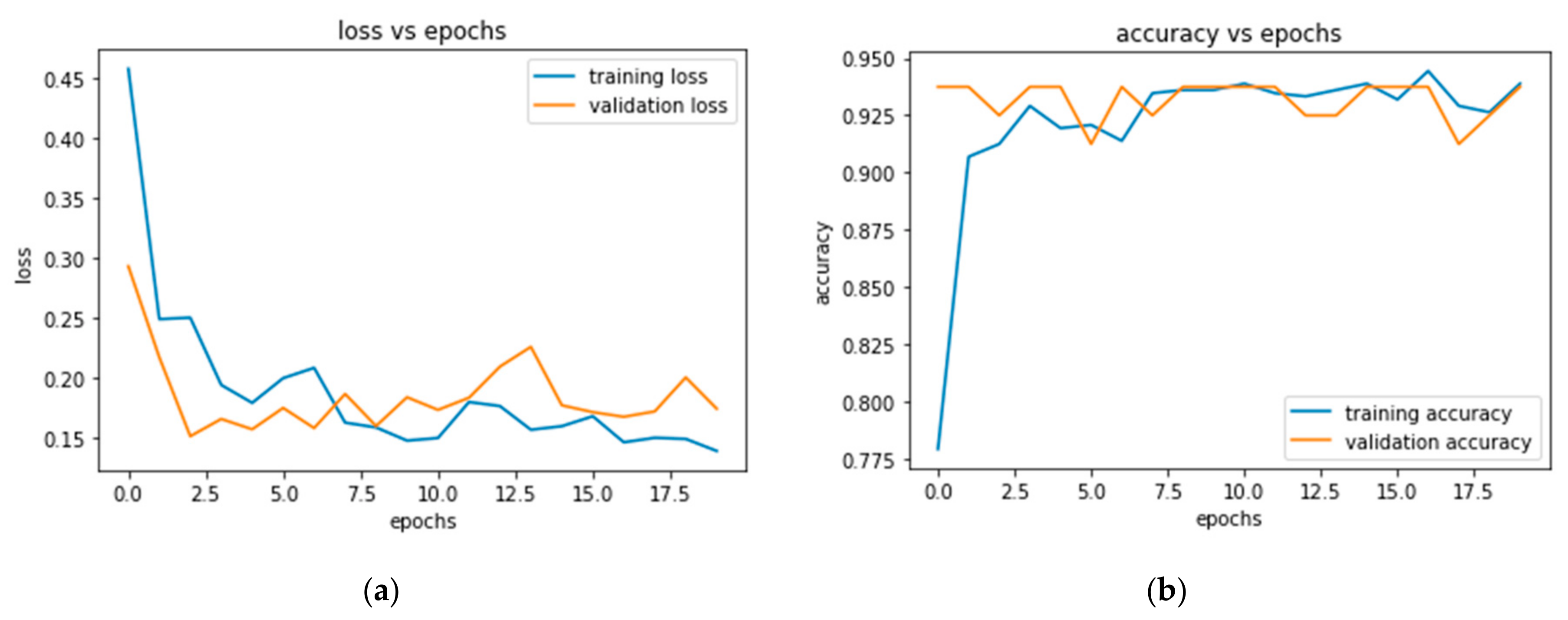
- The effects of the number of iterations per epoch during the training of our proposed deep learning model are analyzed by its each epoch accuracy, data loss, complete training time, and data validation;
- The time-series analysis of the proposed model in terms of data loss and accuracy score among each epoch utilized in the model building;
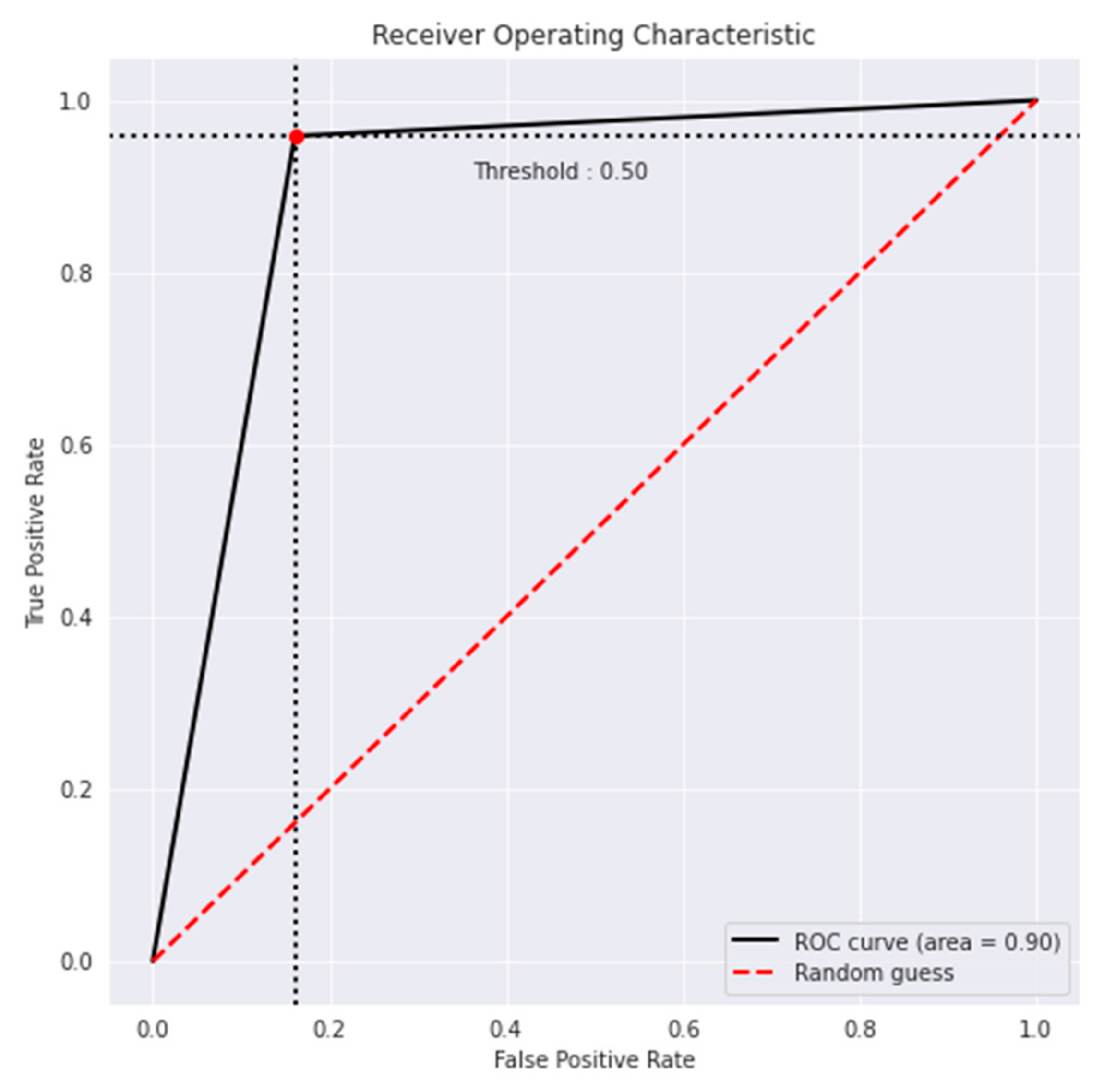
- The ROC (receiver operating characteristic) curve analyses our novel deep-learning-based model at different threshold levels of the asteroseismology target category.
2. Related Work
3. Methodology
3.1. Asteroseismology Dataset
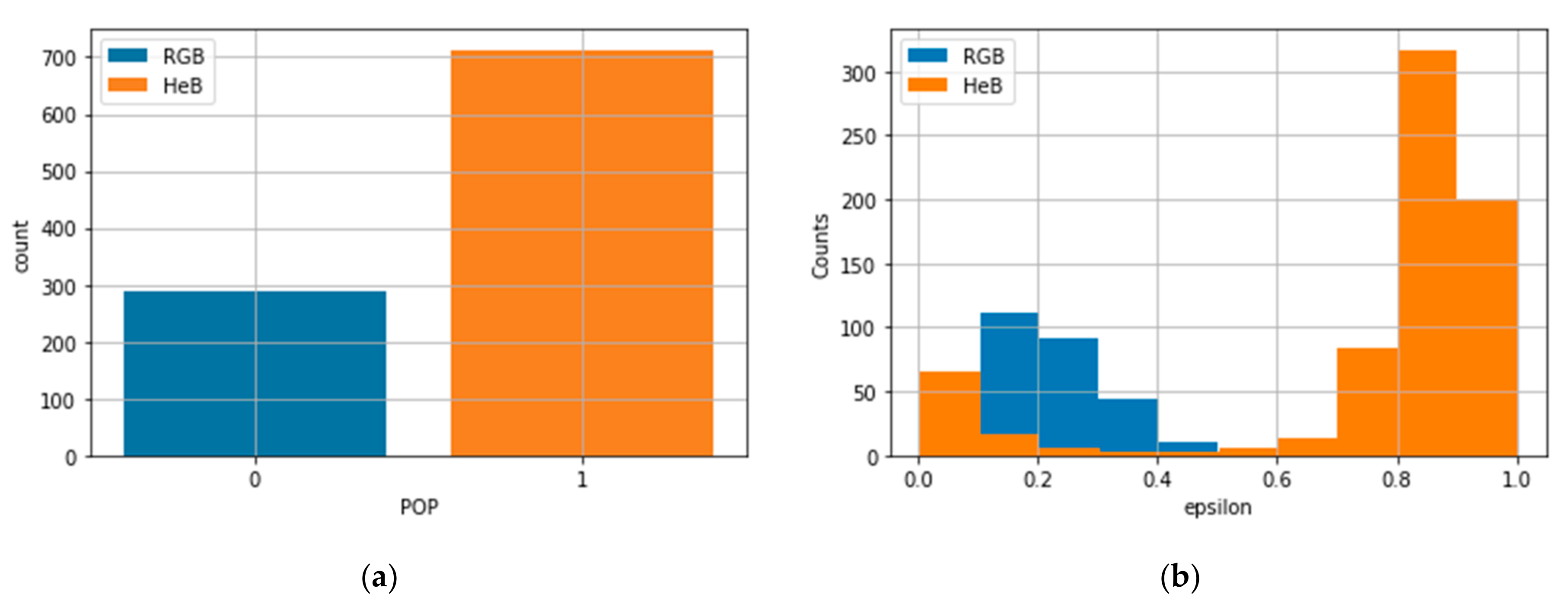
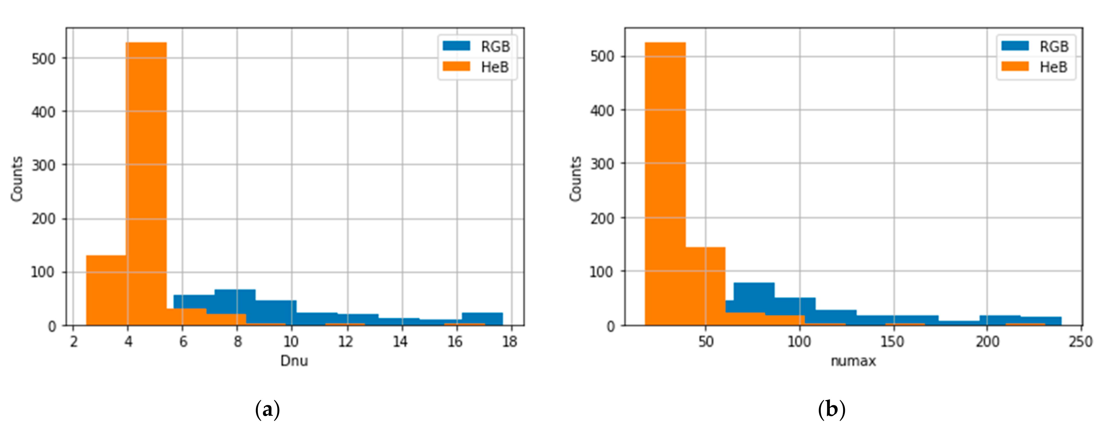
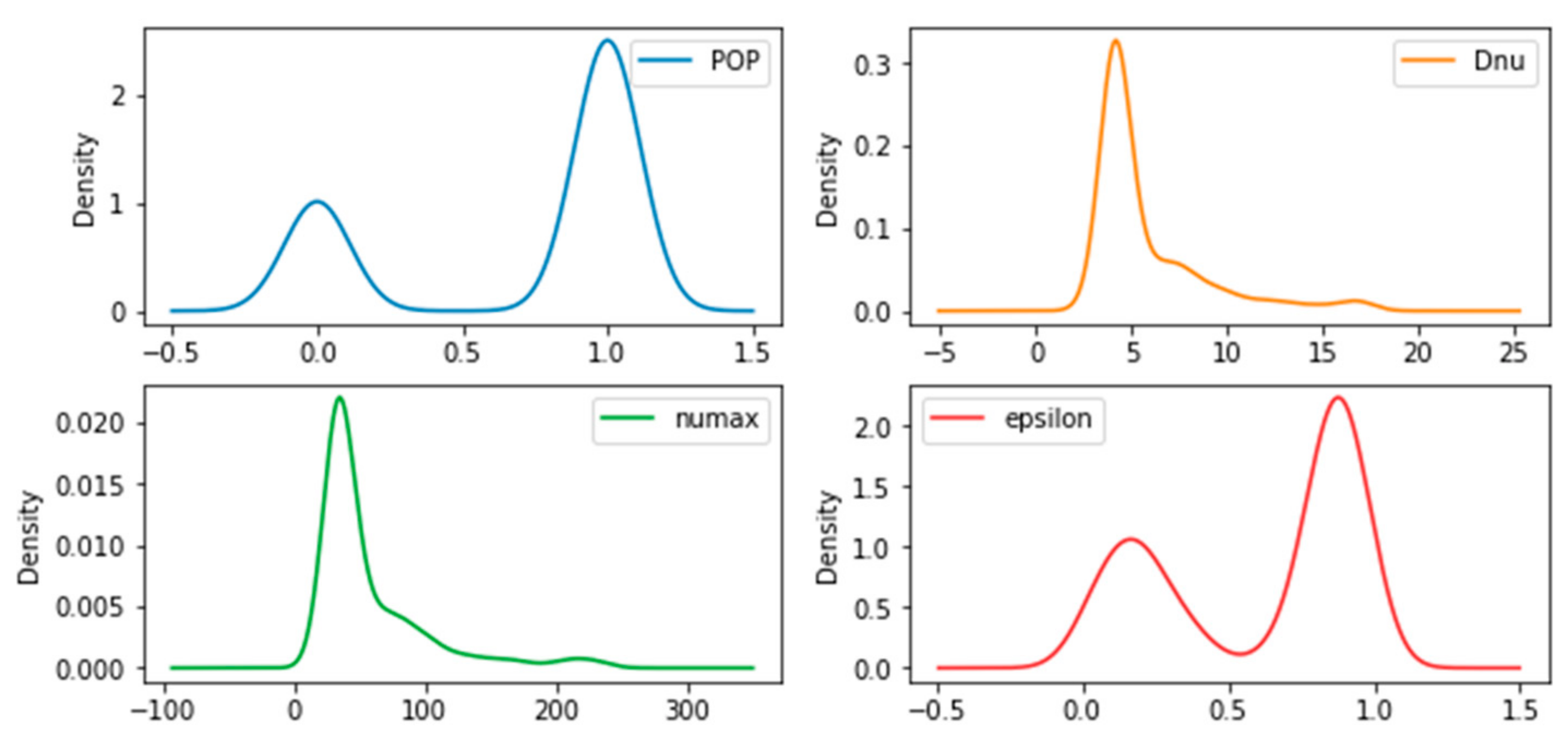
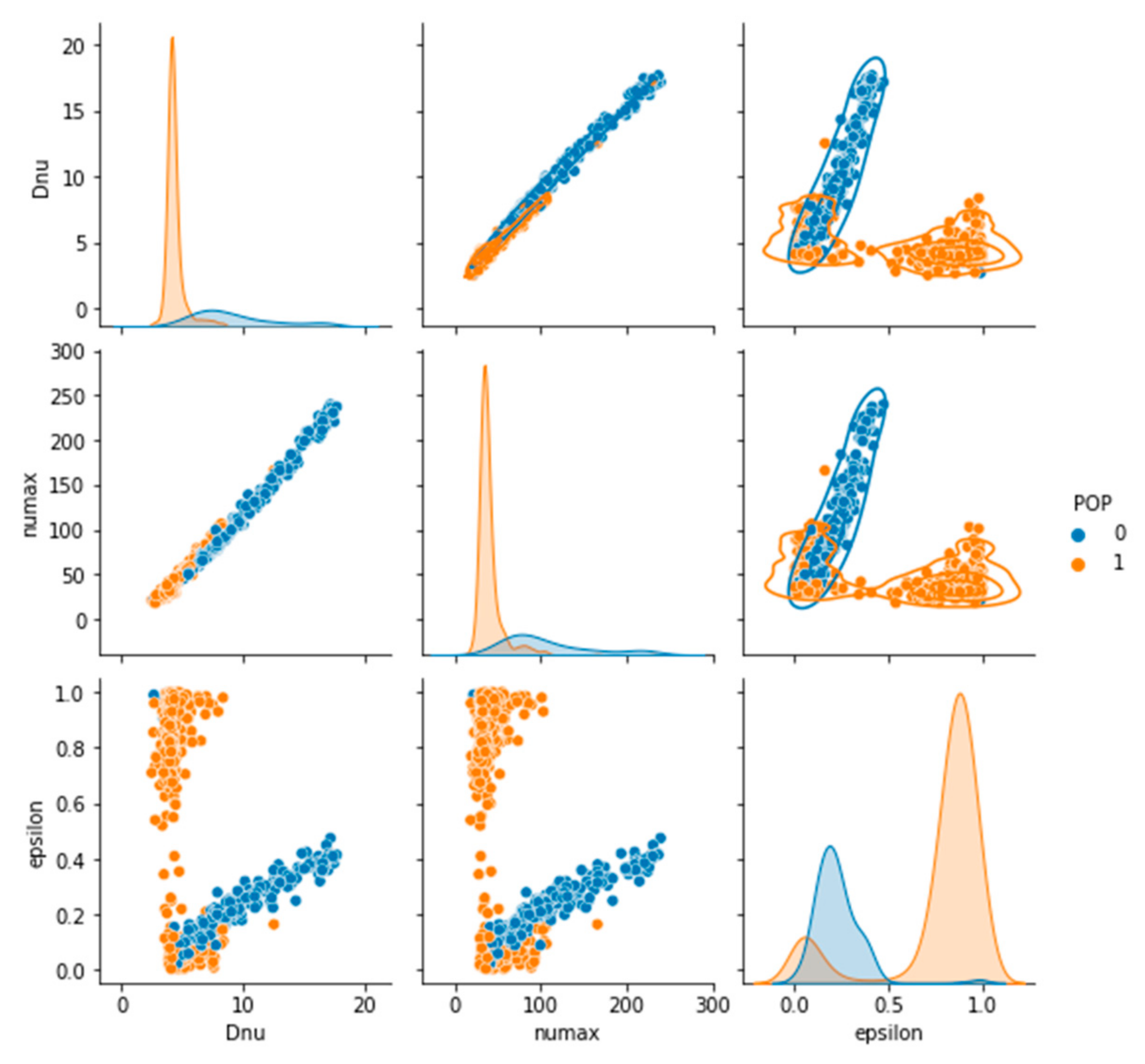
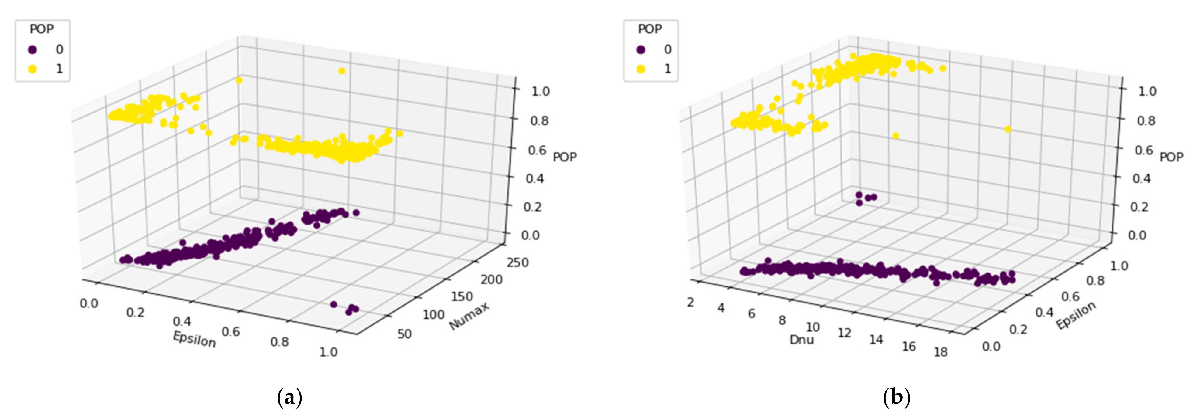
3.2. Asteroseismology Exploratory Data Analysis (AEDA)
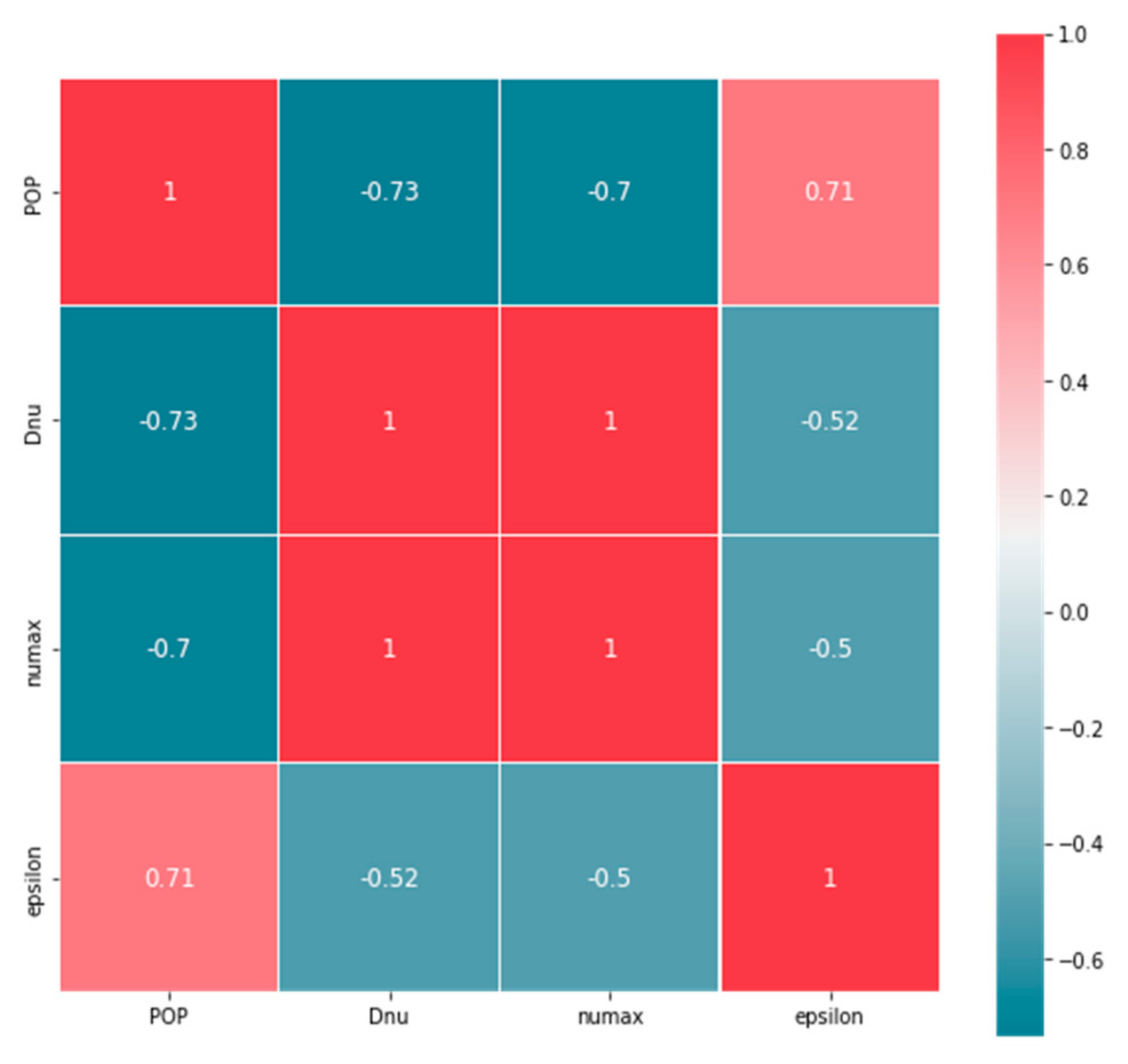
3.3. Asteriosismolgy Dataset Feature Analysis
3.4. Asteroseismology Dataset Splitting
4. Proposed BiGR Approach
4.1. The BiGR Model Configuration Hyperparameter Parameters
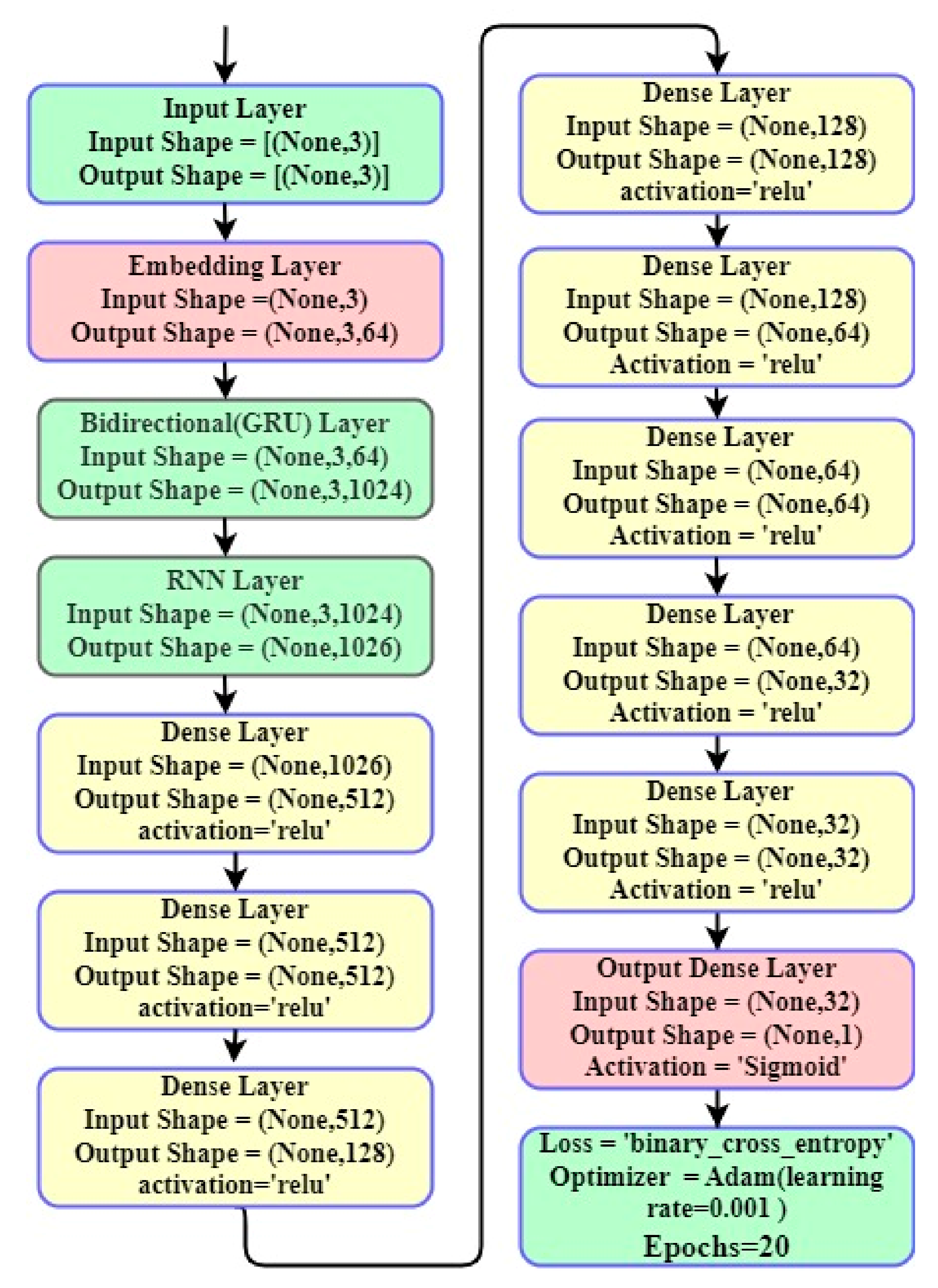
4.2. The BiGR Layers Architecture Analysis
5. Results and Evaluations
6. Conclusions
Author Contributions
Funding
Institutional Review Board Statement
Informed Consent Statement
Data Availability Statement
Acknowledgments
Conflicts of Interest
References
- Aerts, C. Probing the interior physics of stars through asteroseismology. Rev. Mod. Phys. 2021, 93, 015001. [Google Scholar] [CrossRef]
- Zhivanovich, I.; Solov’ev, A.A.; Efremov, V.I. Differential Rotation of the Sun, Helioseismology Data, and Estimation of the Depth of Superconvection Cells. Geomagn. Aeron. 2021, 61, 940–948. [Google Scholar] [CrossRef]
- Di Luzio, L.; Fedele, M.; Giannotti, M.; Mescia, F.; Nardi, E. Stellar evolution confronts axion models. J. Cosmol. Astropart. Phys. 2022, 2022, 35. [Google Scholar] [CrossRef]
- Merlov, A.; Bear, E.; Soker, N. A Red Giant Branch Common-envelope Evolution Scenario for the Exoplanet WD 1856 b. Astrophys. J. Lett. 2021, 915, L34. [Google Scholar] [CrossRef]
- Tillman, N.T. Red Giant Stars: Facts, Definition & the Future of the Sun|Space. Available online: https://www.space.com/22471-red-giant-stars.html (accessed on 15 May 2022).
- COSMOS. Stellar Evolution. Available online: https://astronomy.swin.edu.au/cosmos/s/Stellar+Evolution (accessed on 15 May 2022).
- Li, Y.; Bedding, T.R.; Murphy, S.J.; Stello, D.; Chen, Y.; Huber, D.; Joyce, M.; Marks, D.; Zhang, X.; Bi, S.; et al. Discovery of post-mass-transfer helium-burning red giants using asteroseismology. Nat. Astron. 2022, 6, 673–680. [Google Scholar] [CrossRef]
- Janiesch, C.; Zschech, P.; Heinrich, K. Machine learning and deep learning. Electron. Mark. 2021, 31, 685–695. [Google Scholar] [CrossRef]
- Bartlett, P.L.; Montanari, A.; Rakhlin, A. Deep learning: A statistical viewpoint. Acta Numer. 2021, 30, 87–201. [Google Scholar] [CrossRef]
- Osipov, A.; Pleshakova, E.; Gataullin, S.; Korchagin, S.; Ivanov, M.; Finogeev, A.; Yadav, V. Deep Learning Method for Recognition and Classification of Images from Video Recorders in Difficult Weather Conditions. Sustainability 2022, 14, 2420. [Google Scholar] [CrossRef]
- Gul, F.; Mir, I.; Alarabiat, D.; Alabool, H.M.; Abualigah, L.; Mir, S. Implementation of bio-inspired hybrid algorithm with mutation operator for robotic path planning. J. Parallel Distrib. Comput. 2022, 169, 171–184. [Google Scholar] [CrossRef]
- Ananthanarayana, T.; Srivastava, P.; Chintha, A.; Santha, A.; Landy, B.; Panaro, J.; Webster, A.; Kotecha, N.; Sah, S.; Sarchet, T.; et al. Deep Learning Methods for Sign Language Translation. ACM Trans. Access. Comput. 2021, 14, 1–30. [Google Scholar] [CrossRef]
- Chang, Y.-L.; Tan, T.-H.; Lee, W.-H.; Chang, L.; Chen, Y.-N.; Fan, K.-C.; Alkhaleefah, M. Consolidated Convolutional Neural Network for Hyperspectral Image Classification. Remote Sens. 2022, 14, 1571. [Google Scholar] [CrossRef]
- Trinh Van, L.; Dao Thi Le, T.; Le Xuan, T.; Castelli, E. Emotional Speech Recognition Using Deep Neural Networks. Sensors 2022, 22, 1414. [Google Scholar] [CrossRef]
- Vescovi, D. Mixing and Magnetic Fields in Asymptotic Giant Branch Stars in the Framework of FRUITY Models. Universe 2021, 8, 16. [Google Scholar] [CrossRef]
- Lin, B. Regularity Normalization: Neuroscience-Inspired Unsupervised Attention across Neural Network Layers. Entropy 2021, 24, 59. [Google Scholar] [CrossRef] [PubMed]
- Lee, K.H.; Min, J.Y.; Byun, S. Electromyogram-Based Classification of Hand and Finger Gestures Using Artificial Neural Networks. Sensors 2021, 22, 225. [Google Scholar] [CrossRef]
- Corchado, J.M.; Hussein, F.; Mughaid, A.; Alzu’bi, S.; El-Salhi, S.M.; Abuhaija, B.; Abualigah, L.; Gandomi, A.H. Hybrid CLAHE-CNN Deep Neural Networks for Classifying Lung Diseases from X-ray Acquisitions. Electronics 2022, 11, 3075. [Google Scholar] [CrossRef]
- Mehmet Bilal, E.R. Heart sounds classification using convolutional neural network with 1D-local binary pattern and 1D-local ternary pattern features. Appl. Acoust. 2021, 180, 108152. [Google Scholar] [CrossRef]
- Hon, M.; Stello, D.; Yu, J. Deep learning classification in asteroseismology. Mon. Not. R. Astron. Soc. 2017, 469, 4578–4583. [Google Scholar] [CrossRef]
- Elaziz, M.A.; Ewees, A.A.; Al-qaness, M.A.A.; Abualigah, L.; Ibrahim, R.A. Sine–Cosine-Barnacles Algorithm Optimizer with disruption operator for global optimization and automatic data clustering. Expert Syst. Appl. 2022, 207, 117993. [Google Scholar] [CrossRef]
- Elsworth, Y.; Hekker, S.; Basu, S.; Davies, G.R. A new method for the asteroseismic determination of the evolutionary state of red-giant stars. Mon. Not. R. Astron. Soc. 2017, 466, 3344–3352. [Google Scholar] [CrossRef]
- Mughaid, A.; AlZu’bi, S.; Alnajjar, A.; AbuElsoud, E.; Salhi, S.E.; Igried, B.; Abualigah, L. Improved dropping attacks detecting system in 5g networks using machine learning and deep learning approaches. Multimed. Tools Appl. 2022, 1–23. [Google Scholar] [CrossRef]
- Cao, B.; Li, C.; Song, Y.; Qin, Y.; Chen, C. Network Intrusion Detection Model Based on CNN and GRU. Appl. Sci. 2022, 12, 4184. [Google Scholar] [CrossRef]
- Liu, K.; Hu, X.; Zhou, H.; Tong, L.; Widanage, W.D.; Marco, J. Feature Analyses and Modeling of Lithium-Ion Battery Manufacturing Based on Random Forest Classification. IEEE/ASME Trans. Mechatron. 2021, 26, 2944–2955. [Google Scholar] [CrossRef]
- Amanat, A.; Rizwan, M.; Javed, A.R.; Abdelhaq, M.; Alsaqour, R.; Pandya, S.; Uddin, M. Deep Learning for Depression Detection from Textual Data. Electronics 2022, 11, 676. [Google Scholar] [CrossRef]
- Gilliland, R.L.; McCullough, P.R.; Nelan, E.P.; Brown, T.M.; Charbonneau, D.; Nutzman, P.; Christensen-Dalsgaard, J.; Kjeldsen, H. Asteroseismology of the transiting exoplanet host hd 17156 with hubble space telescope fine guidance sensor. Astrophys. J. 2010, 726, 2. [Google Scholar] [CrossRef]
- Filho, F.J.S.L. Classification in Asteroseismology | Kaggle. Available online: https://www.kaggle.com/datasets/fernandolima23/classification-in-asteroseismology (accessed on 15 May 2022).
- Oxford Academic. Deep Learning Classification in Asteroseismology | Monthly Notices of the Royal Astronomical Society. Available online: https://academic.oup.com/mnras/article/469/4/4578/3828087#supplementary-data (accessed on 15 May 2022).
- Zulqarnain, M.; Ghazali, R.; Hassim, Y.M.M.; Aamir, M. An Enhanced Gated Recurrent Unit with Auto-Encoder for Solving Text Classification Problems. Arab. J. Sci. Eng. 2021, 46, 8953–8967. [Google Scholar] [CrossRef]
- Nwakanma, C.I.; Islam, F.B.; Maharani, M.P.; Kim, D.S.; Lee, J.M. IoT-Based Vibration Sensor Data Collection and Emergency Detection Classification using Long Short Term Memory (LSTM). In Proceedings of the 2021 International Conference on Artificial Intelligence in Information and Communication (ICAIIC), Jeju Island, Korea, 13–16 April 2021; pp. 273–278. [Google Scholar] [CrossRef]
- Vatsya, R.; Ghose, S.; Singh, N.; Garg, A. Toxic Comment Classification Using Bi-directional GRUs and CNN. Lect. Notes Data Eng. Commun. Technol. 2022, 91, 665–672. [Google Scholar] [CrossRef]
- Qi, W.; Ovur, S.E.; Li, Z.; Marzullo, A.; Song, R. Multi-Sensor Guided Hand Gesture Recognition for a Teleoperated Robot Using a Recurrent Neural Network. IEEE Robot. Autom. Lett. 2021, 6, 6039–6045. [Google Scholar] [CrossRef]
- Khan, M.A. HCRNNIDS: Hybrid Convolutional Recurrent Neural Network-Based Network Intrusion Detection System. Processes 2021, 9, 834. [Google Scholar] [CrossRef]
- Rao, S.; Narayanaswamy, V.; Esposito, M.; Thiagarajan, J.; Spanias, A. Deep Learning with hyper-parameter tuning for COVID-19 Cough Detection. In Proceedings of the 2021 12th International Conference on Information, Intelligence, Systems & Applications (IISA), Chania Crete, Greece, 12–14 July 2021. [Google Scholar] [CrossRef]
- Hamm, C.A.; Wang, C.J.; Savic, L.J.; Ferrante, M.; Schobert, I.; Schlachter, T.; Lin, M.D.; Duncan, J.S.; Weinreb, J.C.; Chapiro, J.; et al. Deep learning for liver tumor diagnosis part I: Development of a convolutional neural network classifier for multi-phasic MRI. Eur. Radiol. 2019, 29, 3338–3347. [Google Scholar] [CrossRef]
- de Groof, A.J.; Struyvenberg, M.R.; van der Putten, J.; van der Sommen, F.; Fockens, K.N.; Curvers, W.L.; Zinger, S.; Pouw, R.E.; Coron, E.; Baldaque-Silva, F.; et al. Deep-Learning System Detects Neoplasia in Patients with Barrett’s Esophagus with Higher Accuracy Than Endoscopists in a Multistep Training and Validation Study with Benchmarking. Gastroenterology 2020, 158, 915–929.e4. [Google Scholar] [CrossRef] [PubMed]
- Reddy, V.S.M.; Poovizhi, T. A Novel Method for Enhancing Accuracy in Mining Twitter Data Using Naive Bayes over Logistic Regression. In Proceedings of the 2022 International Conference on Business Analytics for Technology and Security (ICBATS), Dubai, United Arab Emirates, 16–17 February 2022. [Google Scholar] [CrossRef]


| Literature | Year of Publication | Data Set | Learning Type | Proposed Technique | Research Aim |
|---|---|---|---|---|---|
| [22] | 2016 | Kepler satellite | Data Analysis | Novel Method | A new method was proposed for classification to determine the evolutionary phase of HeB and RGB stars. |
| [20] | 2017 | Asteroseismology | Deep Learning | 1D CNN | Simple deep-learning-based 1D CNN was proposed for classification in asteroseismology. |
| [24] | 2022 | UNSW_NB15 | Deep Learning | CNN-GRU | The deep-learning-based CNN and GRU models were proposed for network intrusion classification. |
| [26] | 2022 | Scraped Depression Tweets | Deep Learning | RNN | The classification of depression from Twitter tweets using the deep-learning-based RNN model. |
| Proposed | 2022 | Asteroseismology | Deep Learning | BiGR | A novel deep-learning-based BiGR approach is proposed in the context of asteroseismology classification. |
| Sr no. | Column | Non-Null Count | Data Type | Description |
|---|---|---|---|---|
| 1 | POP | 1001 | Int64 | Population as follows: 0 = RGB, 1 = HeB. The RGB (Red Giant Branch) and HeB (Helium Burning) are in their full forms. |
| 2 | Dnu | 1001 | Float64 | Dnu F8.5 (uHz) Mean significant frequency separation of modes with the same degree and consecutive order, {DELTA}nu. |
| 3 | Numax | 1001 | Float64 | numax F9.5 (uHz) Frequency of maximum oscillation power. |
| 4 | Epsilon | 1001 | Float64 | epsilon F7.3 Location of the l = 0 mode. |
| Index | POP | Dnu | Numax | Epsilon |
|---|---|---|---|---|
| 0 | 1 | 4.44780 | 43.06289 | 0.985 |
| 1 | 0 | 6.94399 | 74.07646 | 0.150 |
| 2 | 1 | 2.64571 | 21.57891 | 0.855 |
| 3 | 1 | 4.24168 | 32.13189 | 0.840 |
| 4 | 0 | 10.44719 | 120.37356 | 0.275 |
| Features | Count | Mean | STD | Min | 25% | 50% | 75% | Max |
|---|---|---|---|---|---|---|---|---|
| POP | 1001.0 | 0.712288 | 0.452923 | 0.00000 | 0.00000 | 1.00000 | 1.00000 | 1.00000 |
| Dnu | 1001.0 | 5.774810 | 2.998103 | 2.50008 | 4.07316 | 4.30874 | 6.58034 | 17.69943 |
| Numax | 1001.0 | 58.441771 | 43.425561 | 17.97978 | 32.92435 | 38.29316 | 70.14083 | 239.64848 |
| Epsilon | 1001.0 | 0.610774 | 0.342518 | 0.00500 | 0.22000 | 0.81500 | 0.89000 | 1.00000 |
| POP | Mean Values | ||
|---|---|---|---|
| Dnu | Numax | Epsilon | |
| 0 | 9.231920 | 106.477706 | 0.227222 |
| 1 | 4.378389 | 39.038756 | 0.765701 |
| Sr no. | Model Layers | Unit | Activation | Output Shape | Parameters |
|---|---|---|---|---|---|
| 1 | The Feature Embedding layers. | 50,000 | N/A | (None, 3, 64) | 3,200,000 |
| 2 | The Bidirectional-Gated recurrent unit layers. | 512 | N/A | (None, 3, 1024) | 1,775,616 |
| 3 | The Recurrent neural networks layers. | 1026 | N/A | (None, 1024) | 2,104,324 |
| 4 | The Dense layers. | 512 | RELU | (None, 512) | 525,824 |
| 5 | The Dense layers. | 512 | RELU | (None, 512) | 262,656 |
| 6 | The Dense layers. | 128 | RELU | (None, 128) | 65,664 |
| 7 | The Dense layers. | 128 | RELU | (None, 128) | 16,512 |
| 8 | The Dense layers. | 64 | RELU | (None, 64) | 8256 |
| 9 | The Dense layers. | 64 | RELU | (None, 64) | 4160 |
| 10 | The Dense layers. | 32 | RELU | (None, 32) | 2080 |
| 11 | The Dense layers. | 32 | RELU | (None, 32) | 1056 |
| 12 | The Dense layers. | 1 | SIGMOID | (None, 1) | 33 |
| Epoch | Training Time/Step | Training Loss | Training Accuracy | Validation Loss | Validation Accuracy |
|---|---|---|---|---|---|
| 1 | 10 s 214 ms | 0.4574 | 0.7792 | 0.2926 | 0.9375 |
| 2 | 4 s 160 ms | 0.2485 | 0.9069 | 0.2166 | 0.9375 |
| 3 | 4 s 160 ms | 0.2497 | 0.9125 | 0.1508 | 0.9250 |
| 4 | 4 s 172 ms | 0.1936 | 0.9292 | 0.1652 | 0.9375 |
| 5 | 4 s 165 ms | 0.1786 | 0.9194 | 0.1566 | 0.9375 |
| 6 | 4 s 162 ms | 0.1993 | 0.9208 | 0.1744 | 0.9125 |
| 7 | 4 s 162 ms | 0.2078 | 0.9139 | 0.1576 | 0.9375 |
| 8 | 4 s 164 ms | 0.1621 | 0.9347 | 0.1861 | 0.9250 |
| 9 | 4 s 165 ms | 0.1581 | 0.9361 | 0.1593 | 0.9375 |
| 10 | 4 s 164 ms | 0.1471 | 0.9361 | 0.1833 | 0.9375 |
| 11 | 4 s 164 ms | 0.1493 | 0.9389 | 0.1728 | 0.9375 |
| 12 | 4 s 189 ms | 0.1793 | 0.9347 | 0.1828 | 0.9375 |
| 13 | 4 s 162 ms | 0.1760 | 0.9333 | 0.2089 | 0.9250 |
| 14 | 4 s 159 ms | 0.1562 | 0.9361 | 0.2254 | 0.9250 |
| 15 | 4 s 163 ms | 0.1591 | 0.9389 | 0.1766 | 0.9375 |
| 16 | 4 s 160 ms | 0.1674 | 0.9319 | 0.1708 | 0.9375 |
| 17 | 4 s 160 ms | 0.1457 | 0.9444 | 0.1670 | 0.9375 |
| 18 | 4 s 159 ms | 0.1495 | 0.9292 | 0.1715 | 0.9125 |
| 19 | 4 s 161 ms | 0.1485 | 0.9264 | 0.1999 | 0.9250 |
| 20 | 4 s 162 ms | 0.1385 | 0.9389 | 0.1738 | 0.9375 |
| Proposed Model | Performance Metrics | |||||||
|---|---|---|---|---|---|---|---|---|
| Epoch | Training Accuracy % | Testing Accuracy % | Precision% | Recall% | F1 Score% | ROC Accuracy % | Log Loss | |
| BiGR | 5 | 72 | 69 | 48 | 69 | 57 | 50 | 10.6 |
| Proposed Model | Performance Metrics | |||||||
|---|---|---|---|---|---|---|---|---|
| Epoch | Training Accuracy % | Testing Accuracy % | Precision% | Recall% | F1 Score% | ROC Accuracy % | Log Loss | |
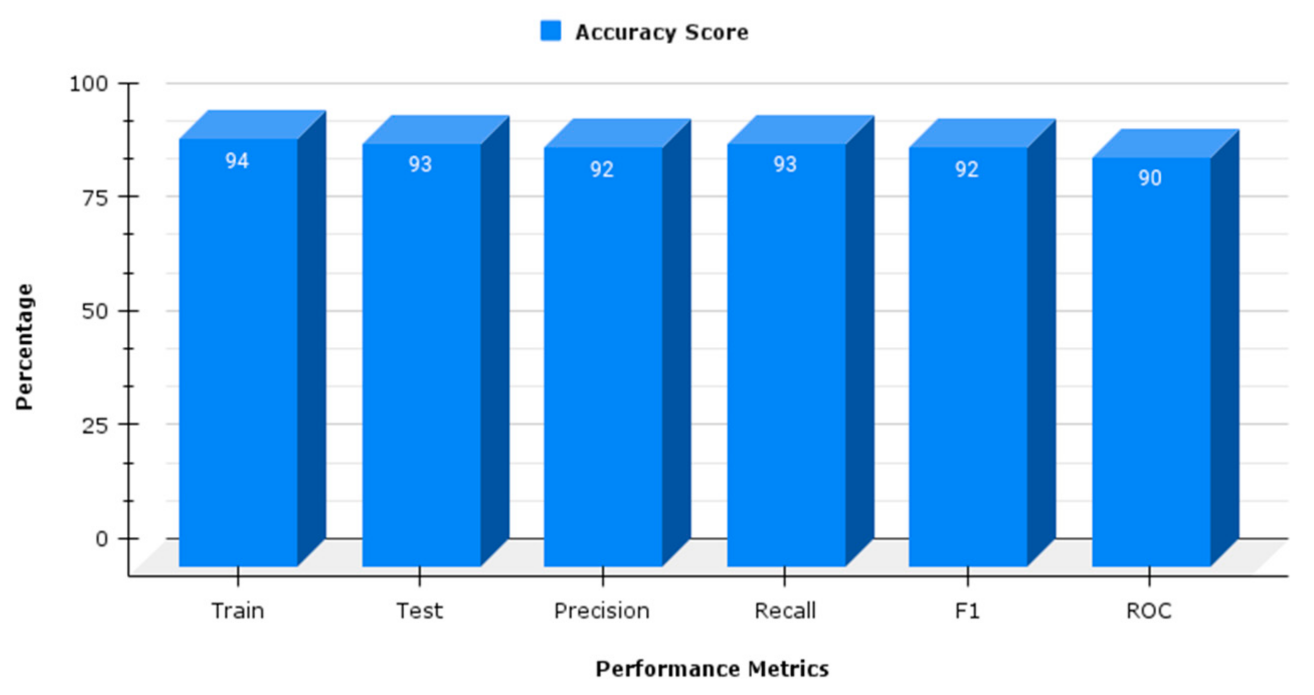
| BiGR | 20 | 94 | 93 | 92 | 93 | 92 | 90 | 2.5 |
| Category | Performance Metrics | |||
|---|---|---|---|---|
| Precision % | Recall % | F1 Score % | Support Score | |
| 0 | 89 | 84 | 86 | 56 |
| 1 | 94 | 96 | 95 | 145 |
| Average Case | Performance Metrics | |||
|---|---|---|---|---|
| Precision % | Recall % | F1 Score % | Support Score | |
| Macro Average | 91 | 90 | 91 | 201 |
| Weighted Average | 92 | 93 | 92 | 201 |
Publisher’s Note: MDPI stays neutral with regard to jurisdictional claims in published maps and institutional affiliations. |
© 2022 by the authors. Licensee MDPI, Basel, Switzerland. This article is an open access article distributed under the terms and conditions of the Creative Commons Attribution (CC BY) license (https://creativecommons.org/licenses/by/4.0/).
Share and Cite
Raza, A.; Munir, K.; Almutairi, M.; Younas, F.; Fareed, M.M.S.; Ahmed, G. A Novel Approach to Classify Telescopic Sensors Data Using Bidirectional-Gated Recurrent Neural Networks. Appl. Sci. 2022, 12, 10268. https://doi.org/10.3390/app122010268
Raza A, Munir K, Almutairi M, Younas F, Fareed MMS, Ahmed G. A Novel Approach to Classify Telescopic Sensors Data Using Bidirectional-Gated Recurrent Neural Networks. Applied Sciences. 2022; 12(20):10268. https://doi.org/10.3390/app122010268
Chicago/Turabian StyleRaza, Ali, Kashif Munir, Mubarak Almutairi, Faizan Younas, Mian Muhammad Sadiq Fareed, and Gulnaz Ahmed. 2022. "A Novel Approach to Classify Telescopic Sensors Data Using Bidirectional-Gated Recurrent Neural Networks" Applied Sciences 12, no. 20: 10268. https://doi.org/10.3390/app122010268
APA StyleRaza, A., Munir, K., Almutairi, M., Younas, F., Fareed, M. M. S., & Ahmed, G. (2022). A Novel Approach to Classify Telescopic Sensors Data Using Bidirectional-Gated Recurrent Neural Networks. Applied Sciences, 12(20), 10268. https://doi.org/10.3390/app122010268